implicit second-derivative runge-kutta collocation methods...

288

Adamawa State University Journal of Scientific Research ISSN: 2251-0702 (P)

Volume 6 Number 2, August, 2018; Article no. ADSUJSR 0602032

http://www.adsujsr.com

Implicit Second-Derivative Runge-Kutta Collocation Methods of Uniformly Accurate Order 3

and 4 for the Solution of Systems of Initial Value Problems Skwame, Y.,1 Kumleng, G. M.2 and Zirra, D. J.1 1Department of Mathematics, Adamawa State University, Mubi, Nigeria 2Department of Mathematics, University of Jos, Plateau State, Nigeria

Abstract

We consider the construction of a new class of implicit Second-derivative Runge-Kutta collocation methods

based on intra-step nodal points of Chebyshev-Gauss-Lobatto type, designed for the numerical solution of

systems of initial value equations and show how they have been implemented in an efficient parallel computing

environment. We also discuss the difficulty associated with large systems and how, in this case, one must take

advantage of the second derivative terms in the methods. We involve the introduction of collocation at the two

end points of the integration interval in addition to the Gaussian interior collocation points and also the

introduction of a different class of basic second derivative methods. With these modifications, fewer function

evaluations per step are achieved. The stability properties of these methods are investigated and numerical

results are given for each method.

Keywords: Block hybrid discrete scheme; Continuous scheme; System of equations; Second-derivative Runge-

Kutta methods

Introduction

In this paper, we present a new class of implicit

second-derivative Runge-Kutta (SDRK)

collocation methods for the numerical solution of

initial value problems for systems of ordinary

differential equations (ODEs),

.0

,,,,

o

o

xyy

Txxxyxfxy

(1)

Here

dd

o

d

o xTxfandTxy ,:,:is

assumed to be sufficiently smooth andd

oy is

the given initial value. Let 0h be a constant

step-size and define the grid by

Nnnhxx on ,,2,1,0, where

oxTNh and a set of equally spaced points

on the integration interval is defined by

Txxxxx no 1321 ,,. The

motivation for studying the implicit second-

derivative Runge-Kutta collocation methods,

particularly, the Gauss–Runge–Kutta collocation

family, is that, collocation at the Gauss points leads

to Runge-Kutta methods which are symmetric and

algebraically stable, Burrage and Butcher (1979). It

was also shown in Yakubu (2003, 2010, 2011,

2015, 2016) and Donald, Skwame and Dominic

(2015) that the only symmetric algebraically stable

collocation methods are those based on Gauss

points. The inclusion of the two end points of the

integration interval as collocation points in addition

to the Gaussian interior collocation points make

them more advantageous, because this minimizes

the number of internal function evaluations

necessary to achieve a given order of accuracy.

Secondly, a substantial increase in efficiency

maybe achieved by the numerical integration

methods which utilize the second-derivative terms.

Thirdly, the relatively good stability properties

enjoyed by these methods make them more

efficient for the numerical integration of system

shaving Jacobians with eigenvalues lying close to

the imaginary axis Adesanya, Fotta and Onsachi

(2016) and Akinfenwa, Abdulganiy, Akinnukawe

,Okunuga and Rufai (2017).

In this paper, we follow the approach of Yakubu,

Kumleng and Markus (2017) to derive a class of

efficient implicit second-derivative Runge-Kutta

collocation methods of high order accuracy, which

converge rapidly to the required solutions. We

hope that our study can stimulate further interest

which will lead to a thorough investigation of the

new class of methods.

A General Approach to the Derivation of the

SDRK Collocation Methods

Skwame et al., ADSUJSR, 6(2):288-300, August, 2018

289

In this section, we shall carryout the general

derivation of the special class of implicit second-

derivative Runge-Kutta collocation methods for

direct integration of initial value problems of the

form (1). We consider the multistep collocation

approach of Onumanyi et al., [1994] and now

extends to second derivative of the form,

jn

t

j

jjn

s

j

jjn

r

j

j yxhyxhyxxy

)()()()(1

0

21

0

1

0

. (2)

We set the sum tsrp

where, r denotes the number of interpolation points used, and 0,0 ts

are distinct collocation points.

Here )(xj

, )(xj

and )(xj are parameters of the methods which are to be determined. They are

assumed to be polynomials of the form

ip

i

ijj xx

1

0

1,)( ,

ip

i

ijj xhxh

1

0

1,)( ,

ip

i

ijj xhxh

1

0

1,

22 )( (3)

We find it convenient to introduce the following polynomials

ip

i

i

1

0

)(

,

ip

i

i

1

0

)(

,

ip

i

i

1

0

)(

which we shall call the first, second and third characteristic polynomials respectively of (2).

Here, our aim is to utilize not only the interpolation points }{ jx

but also several collocation points on the

interpolation interval of (2). This means that we employ a special type of Hermite interpolation for ).(xy

Substituting (3) into (2) we have

.

)(

1

0

1

0

1

0

1

0

1,

2

1,1,

1

0

1

0

1,

21

0

1

0

1

0

1

0

1,1,

ip

i

r

j

s

j

t

j

jnijjnijjnij

t

j

p

i

jn

i

ij

r

j

p

i

s

j

p

i

i

jn

i

ijjn

i

ij

xyhyhy

yxhyxhyxxy

(4)

writing

1

0

1

0

1

0

1

0

1,

2

1,1,

p

i

r

j

s

j

t

j

jnijjnijjniji yhyhy

Equation (4) reduces to

1

0

.)(p

i

i

i xxy (5)

Here }{ jnc are collocation points distributed on the step-points array, jny is the interpolation data of

)(xy

on jnjnjn yandyandx ,

are the collocation data of )()( xyandxy

, respectively, on}{ jnc . We

set the sum tsr to be equal top

so as to be able to determine }{ i

in (2) uniquely.

To fix the parameters ),1,,1,0( pii

we impose the following conditions:

(8))1,2,1,0()(

(7))1,2,1,0()(

(6))1,,2,1,0(,)(

tjyc

sjyc

rjyx

jnjn

jnjn

jnjn

In fact, equations (6) to (8) can be expressed in the matrix-vector form by


290

yV (9)

where theyandvectorsptheVmatrixsquarep ,

are defined as follows:

(10)

Tsnnsnnrnn

T

p yyyyyyy 1111,210 ,,,,,,,,,,,,

where 211 ppDandpD

represent first and second derivatives respectively. Similar to

the Vandermonde matrix, V in (9) is non-singular. Consequently, equation (9) has the unique solution given by

1, VUwhereUy (11)

The interpolation polynomial )(xy

in (5) can now be expressed explicitly as follows:

Tpr

j

s

j

t

j

jnpjjnpjjnpj xxxyhyhyxy 121

0

1

0

1

0

1,

2

1,1, ,,,,1)(

. (12)

Recall thattsp

, such that equation (12) becomes

.,,,,1)( 121

0

1

0

1

0

1,

2

1,1,

Ttsrr

j

s

j

t

j

jntsrjjntsrjjntsrj xxxyhyhyxy

(13)

Expanding (13) fully, gives the continuous scheme;

.,,,,1),,,,,,,()( 12

11,1

TtsrT

tnnsnnrnn xxxUyyyyyyxy

where T denotes transpose of the matrix U in (11) and the vector 12 ,,,,1 tsrxxx

.

In the second-derivative methods, we see that, in

addition to the computation of the f -values at the

internal stages in the standard Runge-Kutta

methods Butcher (2014), the modified methods

involve computing g-values, where g is defined by

Butcher and Hojjati (2005) as ,xygxy

the component number i of xyg can be written

as,

.,,2,1, mixyf

y

xyfxyg j

i

ii

According to Chan and Tsai (2010) these methods

can be practical if the costs of evaluating g are

comparable to those in evaluating f and can even be

more efficient than the standard Runge-Kutta

methods if the number of function evaluations is

fewer. It is convenient to rewrite the coefficients of

the defining method (13) evaluated at some points

in the block matrix form as

,ˆ2 YGIAhYFIAhyeY NNn (14)

3

1

3

1

2

11

332

2

1

4

1

3

1

2

11

2432

1

1

5

1

4

1

3

1

2

11

1

1

5

1

4

1

3

112

1

15432

20126200

20126200

543210

543210

1

0

1

p

snsnsnsn

p

nnnn

p

snsnsnsnsn

p

nnnnn

p

snsnsnsnsnsn

p

nnnnnn

p

nnnnnn

xDccc

cDccc

cDxccc

cDcxcxcxc

xxxxxx

xxxxxx

xxxxxx

V


291

,ˆ2

1 YGIbhYFIbhyy N

T

N

T

nn

where

sxsijaA ,

ssijaA

ˆˆ

indicate the

dependence of the stages on the derivatives found

at the other stages and

1

sibb,

1

ˆˆ

sibb

are

vectors of quadrature weights showing how the

final result depends on the derivatives computed at

the various stages, I is the identity matrix of size

equal to the differential equation system to be

solved and N is the dimension of the system. Also

is the Kronecker product of two matrices and e

is the s×1 vector of units. For simplicity, we write

the method in Yakubu (2017) as follows:

,ˆ2 YGAhYhAFyY n (15)

,ˆ2

1 YGbhYFhbyy TT

nn

and the block vectors in sN are defined by

sY

Y

Y

Y

2

1

,

)(

)(

)(

)(2

1

sYf

Yf

Yf

YF

,

)(

)(

)(

)(2

1

sYg

Yg

Yg

YG

. (16)

where s denotes stage values used in the computation of the step 1Y, 2Y

,…, sY.

The coefficients of the Implicit Two-Derivative Runge-Kutta methods can be conveniently represented more

compactly in an extended partitioned Butcher Tableau, of the form

TTb

A

b

Ac

ˆ

ˆ

(17)

where 11 sc

is the abscissa vectors which indicates the position within the step of the stage values.

Methods

Third Order Implicit Second-Derivative Runge-Kutta Collocation Method

For the first implicit second-derivative Runge-Kutta collocation method we define nxx and consider

the zeros of Legendre polynomial of degree two in the symmetric interval 1,1 , which were transformed into

the standard interval 1, nn xx . The proposed continuous scheme in (13) can now be written as,

vnvnunno gxhfxfxhyxxy 1

2

21 (18)

where

1)(0 x

tttth

x 2

1 8122626912

)(

tttth

x 2

2 8122632612

)(

22

1 812324

2)( thttx


292

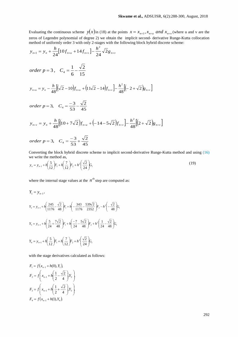
Evaluating the continuous scheme xy in (18) at the points vnunn xandxxx ,1 (where u and v are the

zeros of Legendre polynomial of degree 2) we obtain the implicit second- derivative Runge-Kutta collocation

method of uniformly order 3 with only 2-stages with the following block hybrid discrete scheme:

vnvnunnn gh

ffh

yy 224

141024

2

1

15

2

6

1,3 4 Cporder

vnvnunnun gh

ffh

yy 2248

1421110248

2

45

2

53

3,3 4

Cporder

vnvnunnvn gh

ffh

yy 2248

2514271048

2

45

2

53

3,3 4

Cporder

Converting the block hybrid discrete scheme to implicit second-derivative Runge-Kutta method and using (16)

we write the method as,

1

2

21124

2

12

7

12

5GhFhFhyy nn

(19)

where the internal stage values at the thn step are computed as:

11 nyY ,

1

2

211248

2

2352

2539

1176

343

48

2

1176

245GhFhFhyY n

1

2

211348

2

24

1

48

25

24

7

48

27

24

5GhFhFhyY n

1

2

211424

2

12

7

12

5GhFhFhyY n

with the stage derivatives calculated as follows:

.),1(

,,4

2

2

1

,,4

2

2

1

,),0(

414

313

212

111

YhxfF

YhxfF

YhxfF

YhxfF

n

n

n

n


293

The implicit second-derivative Runge-Kutta collocation method has order p = 3. Writing the method in an

extended Butcher Tableau (16), we have

A Fourth Order Implicit Second-Derivative

Runge-Kutta Collocation Method

Next, as the order of the method being sought for

increases, the algebraic conditions on the

coefficients of the method become increasingly

complicated. However, we consider again the two

end points of the integration interval as collocation

points in addition to the

Gaussian interior collocation points, obtained in the

same manner as in method (18) with the same

02 xp , Legendre polynomial of degree 2.

Thus, the proposed continuous scheme in (13)

takes the

following form:

vnunvnunno gxgxhfxfxhyxxy 21

2

21 (19)

where

1)(0 x

32

1 483124

2)( ttthtx

tttth

x 32

2 483124

2)(

tttttth

x 3222

1 2448283021223648

)(

tttttth

x 3222

2 2448283021223648

)(

Evaluating the proposed continuous scheme xy in (19) at the points vnunn xandxxx ,1 (where u and v

are the zeros of Legendre polynomial of degree 2) we obtain the block hybrid discrete scheme as follows:

vnunvnunnn ggh

ffh

yy 2248

242448

2

1

vnunvnunnun ggh

ffh

yy 2452411384

2669623096384

2

vnunvnunnvn ggh

ffh

yy 2411245384

2309626696384

2

4

22

2352

)249490(

2352

)2532686(

0 0

2352

)2532686(

0

4

22

48

)2710(

48

)2514( 0 0

48

)22( 0

1

24

10 24

14 0 0

24

2 0

24

10 24

14 0 0

24

2 0


294

Solving the block hybrid discrete scheme simultaneously, we obtain the higher order implicit second-derivative

Runge-Kutta collocation method written in the formalism of (15) as follows:

2

2

1

2

21148

2

48

2

2

1

2

1GhGhFhFhyy nn

(20a)

where the internal stage values at the thn step are computed as:

11 nyY ,

2

2

1

2

211296

2

384

5

96

2

384

11

64

211

4

1

64

25

4

1GhGhFhFhyY n

2

2

1

2

211396

2

384

11

96

2

384

5

64

25

4

1

64

25

4

1GhGhFhFhyY n

2

2

1

2

211448

2

48

2

2

1

2

1GhGhFhFhyY n

where the stage derivatives are calculated as follows:

.),1(

,,4

2

2

1

,,4

2

2

1

,),0(

414

313

212

111

YhxfF

YhxfF

YhxfF

YhxfF

n

n

n

n

,

The implicit second-derivative Runge-Kutta collocation method has order p = 4. Writing the method in an

extended Butcher Tableau (16), we have

4

22

384

)23096(

384

)26696(

0 384

)2411(

384

)245( 0

4

22

384

)26696(

384

)23096( 0 384

)245(

384

)2411(

0


295

1

2

1

2

1 0

48

2 48

2 0

2

1

2

1 0 48

2 48

2 0

Analysis of the Second Derivative Runge-Kutta Collocation Methods

Order, Consistency, Zero-stability and Convergence of SDRKC Methods

With the multistep collocation formula (2) we associate the linear difference operator defined by

r

j

s

j

t

j

jjj jhxyxhjhxyxhjhxyxhxy0 0 0

2; (20b)

where xy is an arbitrary function, continuously differentiable on ba, , following Yakubu (2010), we can

write the terms in (20b) as a Taylor series expansion about the point x to obtain the expression,

xyhCxyhCxyhCxyChxy pp

p

)(2

210;

Where the constant coefficients ,2,1,0, pCpare given as follows:

,4,3,!2

1

!1

2

!

1

2!3

1

0 1 0

21

0 1 0

2

3

1 0

2

1

1

0

0

pjp

jp

jp

C

jjC

jC

jC

C

r

j

s

j

t

j

j

p

j

p

jp

r

j

s

j

t

j

jjj

r

j

s

j

jj

r

j

j

r

j

j

According to [24], the multistep collocation formula (2) has order p if

.0,0,; 110

1

pp

p CCCChOhxy

Therefore 1pC is the error constant and

11

1

pp

p yhC is the principal local truncation

error at the point nx (Chan and Tai [2010]).

Therefore, the order and the error constants for the

two methods constructed are represented in Table1.

Table1: Order and error constants of SDRK collocation methods

Method Order Error constant


296

Method (18) 3p

3p

3p

2

4 102383.7 xC 2

4 10597.8 xC 2

4 107617.3 xC

Method (20) 4p 4p 4p

2

5 104583.1 xC 2

5 101193.1 xC 2

5 100547.1 xC

Definition 1: Yakubu and Kwami (2015) The

implicit second-derivative Runge-Kutta collocation

(18) and (20) are said to be consistent if the order

of the individual method is greater than or equal to

one, that is, if .1p

.21

)()(),1()1()(

0)1()(

spolynomialsticcharacterindandstthe

lyrespectivearezandzwhereii

andi

Definition 2:. Yakubu et. al., (2010) The second

derivative Runge-Kutta collocation methods (18)

and ( 20) are said to be zero-stable if the roots

0det0

1

k

i

kiA

Satisfies kjj ,,2,1,1 and for those

roots with 1j , the multiplicity does not

exceed 2.

Definition 3: Yakubu et al., (2010) The necessary

and sufficient conditions for the SDRK collocation

methods (18) and (20) to be convergent are that

they must be consistent and zero-stable.

Stability regions of the SDRK collocation methods In this paper stability properties of the methods are

discussed by reformulating the block hybrid

discrete schemes as general linear methods by

Butcher (2014) and Butcher and Hojjati (2005).

Hence, we use the notations introduced by Butcher

and Hojjati (2005), where a general linear method

is represented by a partitioned rsxrs

matrix (containing A,U, B and V),

Nny

Yhf

VB

UA

y

Y

n

n

n

n

,,2,1,1

(21)

where

,

00

00,00,0

001,

00

,,,,

][

][

2

][

1

][

][

][

2

][

1

][

]1[

]1[

2

]1[

1

]1[

][

][

2

][

1

][

I

I

eI

V

v

BA

Bucu

UBA

A

y

y

y

y

Yf

Yf

Yf

Yf

y

y

y

y

Y

Y

Y

Y

TT

n

r

n

n

n

n

s

n

n

n

n

r

n

n

n

n

s

n

n

n

and ].1,,1[ e

Hence (21 ) takes the form


297

]1[

]1[

2

]1[

1

][

][

2

][

1

][

][

2

][

1

][

][

2

][

1

n

r

n

n

n

s

n

n

n

r

n

n

n

s

n

n

y

y

y

Yhf

Yhf

Yhf

VB

UA

y

y

y

Y

Y

Y

(22)

Where r denotes quantities as output from each step

and input to the next step and s denotes stage

values used in the computation of the step

.,,, 21 syyy The coefficients of these matrices

VandBUA ,,, indicate the relationship

between the various numerical quantities that arise

in the computation of stability regions. The

elements of the matrices VandBUA ,,, are

substituted into the stability matrix which leads to

the recurrent equation hZNnyzMy nn ,1,,3,2,1,1

where the stability matrix

UzAIzBVzM1

and the stability polynomial of the method can

easily be obtained as follows:

.det, 2 BVzUzArz

The absolute stability region of the method is

defined as

.11,: zCx

Computing the stability functions gives the stability polynomials of the methods, which are plotted to produce

the required graphs of the absolute stability regions of the methods as displayed in Fig. 1.

Fig1: Regions of absolute stability of method (18) and method (20) respectively

Remark: The regions of absolute stability of

methods (18) and (20) are stableA since the

region consists of the complex plane outside the

enclosed figures.

Numerical Results

Preliminary numerical experiments have been

carried out using a constant step size

implementation in Matlab. The test examples are

some systems of ordinary differential equations

written as first order initial value problems. We

solved these systems and compared the obtained

results side by side in Tables.

0 0.5 1 1.5 2 2.5 3-2

-1.5

-1

-0.5

0

0.5

1

1.5

2

Re(z)

Im

(z)


298

Example 1:

We consider a well-known classical system which is a mildly stiff problem composed of two first order

equations,

1

1

)0(

)0(,

)(

)(

1999999

1998998

)(

)(

2

1

2

1

2

1

y

y

xy

xy

xy

xy,

and the exact solutions given by the sum of two decaying exponential components

xx

xx

ee

ee

xy

xy

1000

1000

2

1

32

34

)(

)( or

xx

xx

eexy

eexy

1000

2

1000

1

32)(

34)(.

The stiffness ratio is R = 1000 and the problem is

solved numerically on the interval [10,100]. We

have solve the problem using the newly derived

Gauss-Radau-Runge-Kutta collocation methods

and Continuous General Linear methods of Yakubu

(2017) The numerical results obtained are shown in

Table 1, while the region of absolute stability

shown in Fig.1.

Table 1: Absolute errors of numerical solutions of example 1 within the interval 10≤x≤100

x Error in Method (18) Error in Method (20) Error in Yakubu (2010)

Y1 Y2 Y1 Y2 Y1 Y2 10.0 4.684×10

-4 4.4075×10-3 3.452×10

-6 4.607×10-5 4.642×10

-3 4.754×10-3

20.0 5.558×10-6 4.2692 ×10

-6 4.522×10-7 2.728×10

-6 6.808×10-5 9.838×10

-5

30.0 5.689×10-6 2.5522 ×10

-5 6.344×10-8 8.572×10

-8 5.356×10-6 2.078×10

-5 40.0 3.895×10

-6 1.2500 ×10-6 4.255×10

-8 2.029×10-8 3.476×10

-7 3.705×10-6

50.0 1.125×10-7 5.7196 ×10

-6 3.232×10-9 4.464×10

-11 2.107×10-8 6.173×10

-7 60.0 3.223×10

-9 2.5080 ×10-7 3.553×10

-11 9.412×10-12 1.223×10

-9 9.854×10-8

70.0 6.023×10-10

1.0681 ×10-6 5.801×10

-12 1.927×10

-14 6.899×10

-10 1.528×10

-8 80.0 3.457×10

-13 4.4538 ×10

-7 3.422×10-14

3.864×10-16

3.801×10-12

2.320×10-9

90.0 3.470×10-14

1.8272 ×10-8 2.070×10

-16 7.622×10

-18 2.070×10

-13 3.465×10

-10

100 2.441×10-16

7.4021×10-8 1.110×10

-20 1.485×10

-18 1.110×10

-14 5.110×10

-11

Example 2:

Consider the system of mildly stiff linear initial value problem

8)0(,4342

1)0(,78

2212

1211

yyyy

yyyy

Whose exact solution is giving by

)50exp(6)exp(2)(

)50exp()exp(2)(

2

1

xxxy

xxxy

.


299

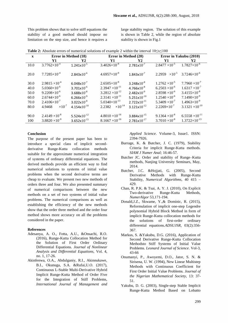
This problem shows that to solve stiff equations the

stability of a good method should impose no

limitation on the step size, and hence it requires a

large stability region. The solution of this example

is shown in Table 2, while the region of absolute

stability is shown in Fig.1

Table 2: Absolute errors of numerical solutions of example 2 within the interval 10≤x≤100

x Error in Method (18) Error in Method (20) Error in Yakubu (2010)

Y1 Y2 Y1 Y2 Y1 Y2

10.0 3.7762×10-4 1.241x10

-5 3.4026×10-8 2.781x10

-7 2.8477 ×10-5 1.7827×10

-6

20.0 7.7285×10

-4 2.843x10-6 4.6957×10

-8 1.843x10-7 2.2959 ×10

-5

3.7246×10

-6

30.0 2.9815 ×10-4 6.048x10

-7 2.6505×10-8 3.248x10

-8 1.2762 ×10-5 7.7960 ×10

-7 40.0 5.0360×10

-6 3.701x10-6 2.3947 ×10

-11 4.766x10-8 6.2503 ×10

-6 1.6317 ×10-7

50.0 9.2208×10-6 3.688x10

-8 3.2812 ×10-12 2.482x10

-9 2.8598 ×10-6 3.4155×10

-8 60.0 2.6744×10

-6 6.266x10-9 2.3141 ×10

-11 5.251x10-10 1.2540 ×10

-6 7.1490×10-9

70.0 2.4106×10-7 3.022x10

-8 5.0340×10

-13 2.722x10-11

5.3409 ×10-7

1.4963×10-9

80.0 4.9468 ×10-7

4.154x10

-10 2.2382 ×10

-14

3.121x10

-12 2.2269×10

-7 3.1321 ×10

-10

90.0 2.4149 ×10-8 5.524x10

-12 4.8010 ×10

-16 3.884x10-15

9.1364 ×10-8

6.5558 ×10-11

100 3.8820 ×10-9 3.652x10

-15 8.1667 ×10

-16 2.781x10-17

3.7010 ×10-8

1.3722×10-13

Conclusion

The purpose of the present paper has been to

introduce a special class of implicit second-

derivative Runge-Kutta collocation methods

suitable for the approximate numerical integration

of systems of ordinary differential equations. The

derived methods provide an efficient way to find

numerical solutions to systems of initial value

problems when the second derivative terms are

cheap to evaluate. We present two new methods of

orders three and four. We also presented summary

of numerical comparisons between the new

methods on a set of two systems of initial value

problems. The numerical comparisons as well as

establishing the efficiency of the new methods

show that the order three method and the order four

method shows more accuracy on all the problems

considered in the paper.

References

Adesanya, A. O., Fotta, A.U., &Onsachi, R.O.

(2016), Runge-Kutta Collocation Method for

the Solution of First Order Ordinary

Differential Equations. Journal of Nonlinear

Analysis and Differential Equations, Vol. 4,

no. 1, 17-26.

Akinfenwa, O.A., Abdulganiy, R.I., Akinnukawe,

B.I., Okunuga, S.A. &Rufai,U.O. (2017),

Continuous L-Stable Multi-Derivative Hybrid

Implicit Runge-Kutta Method of Order Five

for the Integration of Stiff Problems,

International Journal of Management and

Applied Science. Volume-3, Issue1. ISSN:

2394-7926.

Burrage, K. & Butcher, J. C. (1979), Stability

Criteria for implicit Runge-Kutta methods.

SIAM J Numer Anal; 16:46-57.

Butcher JC. Order and stability of Runge–Kutta

methods, Nanjing University Seminars, May,

2014.

Butcher, J.C. &Hojjati, G. (2005), Second

Derivative Methods with Runge-Kutta

Stability, Numerical Algorithms, 40 415 –

429.

Chan, R. P.K. & Tsai, A. Y. J. (2010), On Explicit

Two-derivative Runge-Kutta Methods,

NumerAlgor 53,171-194.

Donald,J.Z., Skwame, Y.,& Dominic, R. (2015),

Reformulation of implicit one-step Legendre

polynomial Hybrid Block Method in form of

implicit Runge-Kutta collocation methods for

the solutions of first-order ordinary

differential equations.ADSUJSR, 03(2):356-

367.

Markus, S. &Yakubu, D.G. (2016), Application of

Second Derivative Runge-Kutta Collocation

Methodsto Stiff Systems of Initial Value

Problems. Leonard Journal of Science. Vol-3,

43-66

Onumanyi, P., Awoyemi, D.O., Jator, S. N. &

Sirisena, U. W. (1994), New Linear Multistep

Methods with Continuous Coefficient for

First Order Initial Value Problems. Journal of

the Nigerian Mathematical Society, 13: 37-

51.

Yakubu, D. G. (2003), Single-step Stable Implicit

Runge-Kutta Method Based on Lobatto


300

Points for Ordinary Differential Equations.

Journal of the Nigerian Mathematical

Society, 22, 57-70.

Yakubu, D.G., Hamza, A. Markus, S., Kwami,

A.M. &Tumba, P. (2010), Uniformly

Accurate Order Five Radau-Runge-Kutta

Collocation Methods. Abacus Journal of

Mathematical Association of Nigeria,

Mathematics series, 372A75-94.

Yakubu, D.G., Manjak, N. H., Buba S.S.,

&Maksha, A. I. (2011), A Family of

Uniformly Accurate Order Runge-Kutta

Collocation Methods, Journal of

Computational and Applied Mathematics,

Vol.30, No.2, Pp 315-330.

Yakubu, D.G.&Kwami, A.M. (2015), Implicit

Two- Derivative Runge-Kutta Collocation

Methods for Systems of Initial Value

Problems. Journal of the Nigerian

Mathematical Society. 34(2):128-142.

Yakubu, D.G., Kumleng, G.M., and Markus,

S.(2017), Second derivative Runge-Kutta

Collocation Methods based on Lobatto nodes

for stiff systems. Journal of modern methods

in numerical mathematics 8:1-2, page 118-

138.

implicit second-derivative runge-kutta collocation methods...

Documents