implicit runge-kutta methods for orbit propagation...implicit runge-kutta methods for orbit...

Implicit Runge-Kutta Methods for Orbit Propagation

Jeffrey M. Aristoff∗ and Aubrey B. Poore†

Numerica Corporation, 4850 Hahns Peak Drive, Suite 200, Loveland, Colorado, 80538, USA

Accurate and efficient orbital propagators are critical for space situational awarenessbecause they drive uncertainty propagation which is necessary for tracking, conjunctionanalysis, and maneuver detection. We have developed an adaptive, implicit Runge-Kutta-based method for orbit propagation that is superior to existing explicit methods, evenbefore the algorithm is potentially parallelized. Specifically, we demonstrate a significantreduction in the computational cost of propagating objects in low-Earth orbit, geosyn-chronous orbit, and highly elliptic orbit. The new propagator is applicable to all regimesof space, and additional features include its ability to estimate and control the truncationerror, exploit analytic and semi-analytic methods, and provide accurate ephemeris datavia built-in interpolation. Finally, we point out the relationship between collocation-basedimplicit Runge-Kutta and Modified Chebyshev-Picard Iteration.

I. Introduction

Accurate and timely surveillance of objects in the near-Earth space environment is becoming increasinglyimportant to national security and presents a unique and formidable challenge. Efficiently and accuratelymodeling trajectories of the vast number of objects in orbit around the Earth is difficult because the equationsof motion are non-linear, the infrequency of observations may require modeling trajectories over long periodsof time, and the number of objects to be modeled is on the order of 105 and growing owing to object breakupsand improved sensors. While existing numerical methods for orbit propagation appear to meet the currentneeds of satellite operators, advances in numerical analysis, together with improved speed, memory, andarchitecture of modern computers (e.g., the availability of parallel processors), necessitate new and improvedalgorithms for orbit propagation, especially when future needs in space situational awareness are taken intoconsideration.

In this paper, we demonstrate the construction, implementation, and performance of collocation-basedimplicit Runge-Kutta (IRK) methods for orbit propagation (i.e., the numerical solution of initial value prob-lems arising in orbital mechanics). This includes collocation-based IRK methods such as Gauss-Legendre,Gauss-Chebyshev, and their Radau and Lobatto variants,1–4 as well as band-limited collocation-based IRKmethods.5,6 Particular attention is given to a class of collocation-based IRK methods known as Gauss-Legendre IRK (GL-IRK). Collocation-based IRK methods are ideally suited for orbit propagation for severalreasons. First, unlike multistep methods, GL-IRK and other collocation-based IRK methods are A-stableat all orders, thus allowing for larger (and fewer) time steps to be taken without sacrificing stability.1–4

As a result, less error is accumulated and the computational cost is reduced. Second, and perhaps moreimportantly, collocation-based IRK methods can exploit parallel computing architectures, which makes themwell-poised to meet the future demands of space surveillance. It is worth noting that current state-of-the-artnumerical integrators such as Dormand-Prince 8(7), Runge-Kutta-Nystrom 12(10), Gauss-Jackson (GJ), andAdams-Bashforth-Moulton (ABM) are explicit methods that are not A-stable nor parallelizable.1–4,7 Theproperties of these methods are summarized in Table 1. A survey of numerical integration methods used fororbit propagation can be found in Montenbruck & Gill8 and Jones & Anderson.9

Our implementation of IRK overcomes the disadvantages often associated with using implicit numericalmethods: the need to solve a system of nonlinear equations at time step. We mitigate this problem by makinguse of available analytic and semi-analytic methods in astrodynamics.8,10 Such approximate solutions are

∗Research Scientist, Numerica Corporation.†Chief Scientist, Numerica Corporation.

1 of 19

American Institute of Aeronautics and Astronautics

DP8(7) RKN12(10) GJ & ABM GL-IRK

Type of method Explicit RK Explicit RK Multistep Implicit RK

Error control Yes Yes No/Yes Yes

Non-conservative forces Yes No Yes Yes

A-stable No No No Yes

Parallelizable No No No Yes

Table 1. Summary of the properties of numerical integration methods used for orbit propagation. While it ispossible to implement error control with Gauss-Jackson (GJ), its standard implementation lacks this feature.7

RKN12(10) is unable to handle cases wherein the force acting on the object depends on its velocity (e.g., whennon-conservative forces are present).

used to warm-start the iterations arising on each time step of IRK, thereby reducing the computationalcost. Second, we have developed an efficient error-control mechanism that allows for the propagation to beentirely adaptivea. Time-adaptivity is achieved through the use of an error estimator which makes use ofthe propagated solution in order to select the optimal time step for a given tolerance, thereby controllingthe accumulation of local error, and minimizing the cost of propagation per time step. This feature, amongothers, distinguishes our work from that of Bai & Junkins,11 Bradley et al.,5 and Beylkin & Sandberg,6 whostudied the use of fixed-step collocation-based methods for orbit propagation.

By virtue of being adaptive, our implementation of IRK is not restricted to the propagation of nearly-circular orbits. Highly elliptic orbits can also be efficiently propagated. Fixed-step propagators, on theother hand, are forced to take extremely small time steps when propagating highly elliptic orbits in order tomaintain high accuracy. Alternatively, the equations of motion can be transformed (e.g., using the Sundmantransform) so that fixed steps can be taken in an orbital anomaly, rather than in time, in an effort todistribute the numerical error evenly across the steps. Unfortunately, this approach results in the need tosolve an additional ordinary differential equation,12 and hence both options incur increased computationalcosts.

This paper focuses on the propagation of objects in low-Earth orbit (LEO), geosynchronous orbit (GEO),and highly elliptic orbit (HEO). The new propagator is found to be superior to existing propagators whenmedium to high accuracy is required. Specifically, we propagate objects in LEO, GEO, and HEO for multipleorbital periods. The performance is compared to that of DP8(7) and ABM, the latter being a method thatis similar to GJ, albeit ABM has error control, whereas the standard implementation of GJ does not haveerror control.7 In a serial computing environment, we demonstrate that the new propagator outperformsDP8(7) and ABM by 60% to 85% in LEO and in GEO, and by 30% to 55% in HEO. In a parallel computingenvironment, the new propagator outperforms DP8(7) and ABM by 92% to 99% in LEO and in GEO, andby 86% to 97% in HEO. Hence, the real impact of the new propagator is its ability to significantly reduce thecomputational cost of orbit propagation, even before the algorithm is potentially parallelized.

The layout of this paper is the following. In Section II, we introduce implicit Runge-Kutta methods anddescribe the construction of collocation-based IRK methods. In Section III, we describe the implementationof adaptive IRK methods for efficient orbit propagation. In Section IV, we compare the performance of ouradaptive collocation-based IRK propagator to that of DP8(7) and ABM. In Section V, we summarize ourresults.

II. Mathematical Preliminaries

The first-order ordinary differential equation (ODE)

y′(t) = f (t,y(t)) , (1)

together with the initial conditiony(t0) = y0, (2)

aAn adaptive numerical method for solving initial value problems estimates the local (truncation) error arising after eachtime step and compares it to a user-specified tolerance to determine whether or not to accept the step, as well as to adjust thesize of the subsequent time step.

2 of 19


define an initial value problem (IVP). Many standard problems in dynamics can be converted to this form.2

The independent variable t (time) is permitted to take on any real value, and the dependent variable y ∈ Rd

(the state of the object) is a vector-valued function y : R → Rd, where d is the dimension of the state,and f : R × Rd → Rd. Henceforth, we assume existence and uniqueness of the solution on some interval[t0, t0 + h].

Runge-Kutta methods may be used to solve the IVP given by (1)-(2), that is, to find the state of theobject at time t = t0 + h.1–4 An s-stage Runge-Kutta method is defined by its weights b = (b1, b2, . . . bs),nodes c = (c1, c2, . . . , cs), and the s by s integration matrix A whose elements are aij . It is used to solvethe IVP over a given time stepb t0 to t0 + h by writing

ξi = f(t0 + cih,y0 + h

s∑j=1

aijξj

)i = 1, 2, . . . , s, (3)

where ξi are the function evaluations at the intermediate times t0 + cih for i = 1, 2, . . . , s, and where theinternal stage zi = y0 +h

∑sj=1 aijξj is the approximation of y at time t0 + cih. Once obtained, the internal

stages are used to advance the solution from t0 to t0 + h according to

y1 = y0 + h

s∑i=1

biξi. (4)

If aij = 0 for i < j, then (3) is an explicit expression for the internal stages. Otherwise, as with implicitRunge-Kutta (IRK) methods, iterative techniques must be used to solve the nonlinear system of equations(3), and an initial guess is required. In fact, as we shall demonstrate in Section III, it is the availabilityof approximate analytical solutions to (1)-(2) that make the iterative solution of (4) tractable in orbitalmechanics. Examples of fixed-point methods for solving (3) include the Jacobi method, the Gauss-Seidelmethod, and the Steffensen method. Newton and quasi-Newton methods can also be used.13 Note thatthe Runge-Kutta method (A, b, c) can be reformulated so that the s evaluations of f in (4) need not beperformed.4

A. Runge-Kutta Methods for Second-Order Systems

Of particular importance in the modeling of the motion of objects subject to forces are equations of the form

Y ′′(t) = g(t,Y (t),Y ′(t)

), (5)

which can be written as a first-order ODE (1) where

y(t) =

(Y (t)

Y ′(t)

)(6)

and

f (t,y(t)) =

(Y ′(t)

g(t,Y (t),Y ′(t)

) ) . (7)

Let the initial condition (2) be

y0 =

(Y 0

Y ′0

). (8)

In this case, the system of equations defining the internal stages of the IRK method (3) becomes

ξi = Y ′0 + h∑s

j=1 aijξ′j

ξ′i = g(t0 + cih,Y 0 + h

∑sj=1 aijξj ,Y

′0 + h

∑sj=1 aijξ

′j

) i = 1, 2, . . . , s, (9)

and (4) becomes

Y 1 = Y 0 + h

s∑i=1

biξi, Y ′1 = Y ′0 + h

s∑i=1

biξ′i. (10)

bTypically, multiple time-steps must be taken to solve an IVP using Runge-Kutta methods.

3 of 19


Substituting the first formula of (9) into the second yields

ξ′i = g(t0 + cih,Y 0 + cihY

′0 + h2

s∑j=1

aijξ′j ,Y

′0 + h

s∑j=1

aijξ′j

), (11)

and substituting the first formula of (9) into (10) yields

Y 1 = Y 0 + hY ′0 + h2s∑

i=1

biξ′i, Y ′1 = Y ′0 + h

s∑i=1

biξ′i. (12)

where

aij =

s∑k=1

aikakj , bi =

s∑j=1

bjaji, and ci =

s∑j=1

aij . (13)

Provided that aij , bi, and ci are pre-computed, these substitutions reduce the storage required by the implicitRunge-Kutta methods as well as the number of iterations.3 Similar substitutions can be done for higher-orderODEs to reformulate the associated IRK method.

B. Construction of Collocation-Based Runge-Kutta Methods

There is an extensive literature devoted to the construction of IRK methods.1–4 Here, we describe theconstruction of a class of IRK methods known as collocation-based IRK methods, which have particularlystrong stability properties. This framework allows us to readily construct collocation-based IRK methodssuch as Gauss-Legendre, Gauss-Chebyshev, and their Radau and Lobatto variants.

Without loss of generalityc, a collocation-based, s-stage IRK method consists of choosing s collocationpoints c1, c2, . . . , cs in [−1, 1], and seeking a vector function u that obeys the initial condition (2) and satisfiesthe differential equation (1) at the collocation points. In other words, one seeks a function u such that

u(t0) = y0

u′(t0 + cih) = f (t0 + cih,u(t0 + cih))i = 1, 2, . . . , s. (14)

A collocation method consists of finding such a u and setting y1 = u(t0 + h). The collocation method forc1, c2, . . . , cs is equivalent to the s-stage IRK method with coefficients

aij =

∫ ci

−1Lj(τ)dτ, i, j = 1, 2, . . . , s, (15)

and

bi =

∫ 1

−1Li(τ)dτ, i = 1, 2, . . . , s, (16)

where

Li(τ) =

s∏`=1, ` 6=i

τ − c`ci − c`

(17)

is the Lagrange interpolating polynomial.Band-limited collocation-based IRK (BLC-IRK) methods,5 and methods wherein the interpolating func-

tion need not be polynomial, may be constructed by choosing a family of orthogonal basis functions andcomputing

aij =

s∑`=1

Ψ−1`j

∫ ci

−1Ψ`(τ)dτ, i, j = 1, 2, . . . , s, (18)

and

bj =

s∑`=1

Ψ−1`j

∫ 1

−1Ψ`(τ)dτ, j = 1, 2, . . . , s, (19)

cThe interval for construction of the IRK method need not be [−1, 1].

4 of 19


whereΨ−1ij = [Ψj(ci)]

−1, i, j = 1, 2, . . . , s (20)

are the components of the interpolation matrix Ψ−1.Collocation-based IRK methods are amenable to interpolation (and extrapolation). The solution of the

IVP at the collocation points, together with the interpolation matrix Ψ−1, the elements of which are givenby (20), can also be used to determine the state of the object at points that do not necessarily correspondto the collocation points.5 Since Ψ−1 can be pre-computed, interpolation can be done efficiently.

C. Other Collocation Methods (e.g., Modified Chebyshev-Picard Iteration)

An alternative, but mathematically equivalent (in the sense that it produces the same discrete approximation)approach to collocation-based IRK is the following.14,15 Rather than working in terms of the values of thefunction f , one works in terms of the coefficients of a chosen family of basis functions Rj for j = 1, 2, . . . , s(e.g., Chebyshev or Legendre polynomials) by expressing the approximate solution u(t) as

u(t) =

s∑j=1

ajRj(t). (21)

The vector coefficients aj are obtained by satisfying the ODE at s chosen collocation points and by satisfyingthe initial condition; the resulting system of nonlinear equations relating the coefficients aj and the function fis solved using iterative techniques. This approach is sometimes referred to as a collocation method, and hasbeen used in astrodynamics by several authors.11,16–18 We emphasize that it is mathematically equivalentto an s-stage collocation-based IRK method having the same collocation points and basis functions,14,15

since this fact does not appear to be well known. Since collocation methods are a subset of IRK methods,we prefer to describe the new propagator in the broader context of IRK. This choice also allows us to easilymake use of a number of results from numerical analysis, most notably, the theory of order conditions.

D. Order Conditions

Let y be the exact solution to the initial value problem (1) and (2) at t = t0+h, and let y1 be an approximatenumerical solution at t = t0 + h. The approximate numerical solution is said to have order p if the localerror satisfies

||y1 − y|| = O(hp+1) (22)

as h→ 0. For an s-stage Runge-Kutta method to obtain order p, it must satisfy the order conditions B(p),C(η), and D(ζ) with p ≤ η + ζ + 1 and p ≤ 2η + 2, where

B(p) :

s∑i=1

bicq−1i =

1

qq = 1, . . . , p; (23)

C(η) :

s∑j=1

aijcq−1j =

cqiq

i = 1, . . . , s, q = 1, . . . , η; (24)

D(ζ) :

s∑i=1

bicq−1i aij =

bjq

(1− cqj) j = 1, . . . , s q = 1, . . . , ζ. (25)

Note that for p = 1, B(p) reduces tos∑

i=1

bi = 1, (26)

which is the condition required for any Runge-Kutta method to be consistent and convergent,1,2 a pre-requisite for its use. Gauss-Legendre IRK methods achieve the highest possible order (p = 2s) and aredeemed super-convergent. Their Radau IA and IIA variants achieve order p = 2s − 1, and their LobattoIIIA, IIIB, and IIIC variants achieve order p = 2s − 2.2,3 Gauss-Chebyshev IRK methods are order p = s.Their Radau IA and IIA variants achieve order p = s − 1, and their Lobatto IIIA, IIIB, and IIIC variantsachieve order p = s − 2.2,3 The order of a BLC-IRK method is between zero and 2s depending upon thechoice of band-limit.

5 of 19


III. Implementation of Implicit Runge-Kutta for Orbit Propagation

One of the main difficulties with the implementation of implicit Runge-Kutta (IRK) methods is the needto solve a nonlinear system of equations at each time step. These must be solved iteratively and in an efficientmanner (see Subsection A), and a stopping criterion for the iterations must be established (see SubsectionB). Moreover, for an IRK method to be practical, approaches to limit the number of iterations should beused that exploit approximate solutions to the initial value problem (see Subsection C). Another difficultywith the implementation of IRK arises from the requirement that the accumulation of error is monitoredand controlled so that the accuracy of the numerical solution can be established (see Subsection D). Thepresent implementation of IRK for orbit propagation addresses and circumvents each of these difficulties.

A. Solution of the Nonlinear System via Fixed-Point Iteration

Newton’s method or one of its many variants can be used for solving the nonlinear system of equations, butthis requires calculation (or approximation) of the Jacobian. In orbit propagation, evaluation of a singlecomponent of the Jacobian is more expensive than evaluation of a single component of the force, and thereare more components to evaluate. Hence, this approach can be costly. Simplified Newton methods avoidhaving to calculate the Jacobian at each of the intermediate times, but reduce the convergence from quadraticto linear.4

Alternatively, fixed-point methods can be used for solving the nonlinear system. Although fixed-pointmethods converge more slowly than Newton’s method (but at the same rate as simplified Newton methods),fixed-point methods do not require the computation of a Jacobian, and are thus well-suited for orbit prop-agation. The downside of using fixed-point methods is that they generally degrade the superior stabilityproperties of IRK methods. In particular, provided that the initial guess is sufficiently close to the solution,there is no limit on the size of the time step that can be taken when a method is A-stable and Newton’smethod is used. If a fixed-point, rather than Newton’s method, is used, then there is a maximum step sizeabove which the iterations diverge. While this may appear to limit the applicability of fixed-point methodsto orbit propagation, we have studied the convergence of fixed-point methods in this context, and determineda bound on the maximum step size, below which the iterations will converge. For the case of unperturbedKeplerian dynamics, our proof of convergence indicates that steps sizes up to three-quarters of an orbitalperiod are acceptable. Practically speaking, the propagator we develop monitors the convergence of theiterations during each step of the propagation, and reduces the step size if necessary.

There are a number of different fixed-point iteration methods that may be used to solve the nonlinearsystem (11), the simplest being the Jacobi method (see Algorithm 1). Note that the s evaluations of the forcemodel and the s internal stage updates can each be done in parallel. An efficient and robust convergencecriteria for stopping the iterations will be presented in Subsection B.

Algorithm 1: Jacobi Method

Jacobi method for solving the nonlinear system (11) arising in orbit propagation.

inputs : Initial guess for the reformulated internal stages zi and z′i, second-order integration matrices and nodes(aij , aij , ci, ci) for i, j = 1, 2, . . . , s, time step h, current state (y0,y

′0), and iteration tolerance.

outputs: Solution for the reformulated internal stages and corresponding force-model evaluations.

beginwhile stopping criterion for the iterations has not been met (see Subsection B) do

for i← 1 to s doEvaluate the force model at node i: g(t0 + cih,y0 + zi,y

′0 + z′i)→ gi.

for i← 1 to s doUpdate the ith internal stage: cihy

′0 + h2

∑sj=1 aijgj → zi and h

∑sj=1 aijgj → z′i.

An alternative to the Jacobi fixed-point method, known as the Gauss-Seidel method (see Algorithm 2),combines the two for-loops of the Jacobi method into a single step. In practice, the Gauss-Seidel methodconverges more quickly because the newly calculated function evaluations are immediately incorporated intothe internal stage updates. However, neither the s evaluations of the force model nor the s internal stageupdates can be done in parallel, so the computational advantages are only obtained in a serial computingenvironment or in a parallel computing environment in which the number of processors does not exceedthe number of orbits to be propagated multiplied by the number of internal stages. In the latter situation,

6 of 19


parallelization at the level of the orbits can still take place, but finer parallelization, at a the level of theinternal stages, cannot.

Algorithm 2: Gauss-Seidel Method

Gauss-Seidel method for solving the nonlinear system (11) arising in orbit propagation.

inputs : Initial guess for the reformulated internal stages zi and z′i and corresponding force-model evaluations,second-order integration matrices and nodes (aij , aij , ci, ci) for i, j = 1, 2, . . . , s, time step h, current state(y0,y



beginwhile stopping criterion for the iterations has not been met (see Subsection B) do

for i← 1 to s doUpdate the ith internal stage: cihy

′0 + h2

∑sj=1 aijgj → zi and h

∑sj=1 aijgj → z′i.

Evaluate the force model at node i: g(t0 + cih,y0 + zi,y′0 + z′i)→ gi.

B. Stopping Criterion for the Iterations

Rather than performing a fixed number of iterations, we seek a stopping criterion that minimizes the numberof iterations necessary for convergence to a given accuracy. Following Hairer & Wanner,4 denote the set ofinternal stages after m iterations as

Vm =

(z1 z2 . . . zs

z′1 z′2 . . . z′s

), (27)

and let ∆Vm = Vm+1 −Vm denote the iteration error. Since convergence is linear, we have

||∆Vm+1|| ≤ Θ||∆Vm||, (28)

where || · || is a suitable matrix norm that is consistent with the way in which the local error is estimated(see Subsection D). Additionally, since we are dealing with a second order system, one must decide whetherto monitor the error Z or Z′ (or some combinationd).

Provided that the iterations are converging (see Subsection A), the convergence rate Θ < 1. Let V∗ bethe exact solution to (11). Applying the triangle inequality to

Vm+1 −V∗ = (Vm+1 −Vm+2) + (Vm+2 −Vm+3) + . . . (29)

yields

||Vm+1 −V∗|| ≤ Θ

1−Θ||∆Vm||. (30)

An estimate of the convergence rate Θ can be made using

Θ = ||∆Vm||/||∆Vm−1||, (31)

or if ∆Vm−1 is unavailable (as is true after only one iteration), Θ from the previous integration step can beused, provided that the previous and current time steps are comparable. We therefore stop the iterationswhen

Θ

1−Θ||∆Vm|| ≤ κ · tol, (32)

and accept Vm+1 as an approximation to V∗, where tol is the local error tolerance and κ is a numericalpre-factor. If Θ ≥ 1 or the number of iterations reaches the maximum allowable number of iterations, wehalt the iterations and reduce the time step by a factor of two.

dNote that the physical dimensions of these matrices differ.

7 of 19


C. Solution of the Nonlinear System Using Multiple Force Models

Physical systems are typically described by a hierarchy of mathematical models of increasing complexity.In orbital mechanics, for example, the complexity of the force model depends upon the degree and orderof the gravity model, and how drag, solar radiation, and third-body effects and other perturbations areaccounted for. It is therefore reasonable to ask whether low- and medium-fidelity force models can be usedin conjunction with high-fidelity force models to efficiently solve differential equations of the form (11). Theanswer depends upon the underlying numerical methods. Implicit numerical methods can exploit multipleforce models, whereas explicit methods cannot.

In particular, the iterative technique used for solving the nonlinear system of equations that arise oneach step of an implicit Runge-Kutta (11), whether it be fixed-point or Newton-step, requires a guess forthe internal stages to start the iterations. Rather than using a single, high-fidelity force model, we use atiered approach wherein multiple force models are evaluated sequentially (see Algorithm 3). This approachsignificantly reduces the number of high-fidelity force-model evaluations, and is similar to the approach usedby Beylkin & Sandberg6 and Bradley et. al.5

Algorithm 3: Sequentially Evaluate Force Models

Sequentially evaluate force models in succession together with IRK to solve the nonlinear system (11) arising inorbit propagation.




begin

Use Algorithm 1 or 2 with g = g(low) where g(low) is a low-fidelity force model, and pass the result as input tothe following step.

Use Algorithm 1 or 2 with g = g(med) where g(med) is a medium-fidelity force model, and pass the result asinput to the following step.

Use Algorithm 1 or 2 with g = g(high) where g(high) is a high-fidelity force model.

D. Error Estimation and Control

Numerical error is intrinsic to orbit propagation (unless the propagation is done analytically). It arisesdue to the finite precision of computations involving floating-point values (i.e., round-off error), and due tothe difference between the exact mathematical solution and the approximation to the exact mathematicalsolution (i.e., truncation error). Owing to round-off error, the final few digits of a floating-point computationcannot be considered to be accurate. Round-off error can be mitigated to some extent,4 but it is truncationerror that is typically the dominant contributor to numerical error in orbit propagation. Recall that thelocal (truncation) error is related to the order of the numerical method (see Section II). Fortunately, thelocal error can be estimated and controlled. Note that the orbital propagators presented by Bradley et al.5

and Bai & Junkins11 do not estimate nor control the error.Modern methods for solving initial value problems (IVPs) estimate and control the error by adjusting

the step size accordingly.19 For higher order methods such as those needed for orbit propagation,8,9 rigorouserror bounds become unpractical, and it is therefore necessary to consider the first non-zero term in theTaylor expansion of the error. Even so, one cannot simply compute the global error (without access tothe true solution), that is, the error of the computed solution after several steps. Rather, the local errorcommitted at each step of the method can be estimated and used to adjust the step size, keeping in mindthat local errors are accumulated and transported to the final state. Ideally, local error control results inglobal error control, and the method takes the largest time steps possible without committing too mucherror. Hence, the method does just the right amount of work solving the IVP.

Let tol = atol+ rtol · ||y0|| be the local error tolerance, where atol is a user-specified absolute tolerance,and rtol is a user-specified relative tolerance. On each step of the propagation, we estimate the local errorand require that it fall below tol. This approach is known as error per step (EPS) controle. The local error

eConversely, error per unit step (EPUS) control requires that the local error fall below tol · h for the step to be accepted.

8 of 19


estimate err is used to adjust the subsequent step according to

hnext = h ·max(0.5,min(2, (0.35 · tol/err)1/(p+1))), (33)

where p is the order of the IRK method (see Section II). The parameters 0.5 and 2 are chosen so that theratio hnext/h is neither too large nor too small. The parameter 0.35 is chosen to increase the probabilitythat the next step is accepted, with the probability depending on the order of the IRK method. We notethat at the culmination of each step, we ensure that the step size to be taken for the following step doesnot exceed the final time. If so, the step size is reduced. Our approach to error control is summarized inAlgorithm 4.

Algorithm 4: Error Estimation and Control

Estimate and control the local error.


′0), iteration tolerance, and local error tolerance.

outputs: Solution for the reformulated internal stages and corresponding force-model evaluations accurate towithin the local error tolerance.

beginwhile step has not been accepted do

Use Algorithm 3 to compute the s-stage IRK step and the error estimate err.if err ≤ tol then

Accept the step. Use (33) to increase or decrease the time step.else

Reject the step. Use (33) to decrease the time step.

We choose to estimate and control the error in propagating an orbit by using Earth-centered-inertialcoordinates (ECI). The reason for this choice is two-fold. First, the components of the internal stagesnaturally separate into positions and velocities in ECI. Then, one simply decides whether to control theerror in position, the error in velocity, or both. Second is the fact that the geopotential calculation and itsderivatives (the component of the force model evaluation that is most expensive) are naturally expressedin Earth-centered-Earth-fixed coordinates, which convert to ECI through a trivial rotation.8 Use of analternative coordinate system for propagation would incur an additional cost due to the necessary changeof variable at each node. Furthermore, one would not be able to exploit the second-order formulation ofimplicit Runge-Kutta to reduce the computational cost of integration.

IV. Performance of the New Orbital Propagator

In this section, we test the performance of the new IRK-based propagator in six realistic orbit propagationscenarios. Both the efficiency and the accuracy of the propagations will be quantified. Although any IRKscheme can be used within the new propagator (including those not based on collocation) we have chosento use the Gauss-Legendre IRK (GL-IRK) family of methods in the present study because:

• GL-IRK methods are A-stable (and B-stable) and can therefore be applied to stiff problems (e.g.,satellite re-entry, highly elliptic orbits),

• GL-IRK methods are parallelizable and can therefore exploit advanced computing architectures (eachevaluation of the force model can be done independently and on a different processor),

• GL-IRK methods are super-convergent, they achieve the highest order of convergence possible for aRunge-Kutta method (methods based on Chebyshev collocation are not super-convergent),

• GL-IRK methods are symmetric and thus preserve time-reversibility of a dynamical system (if appli-cable), and

• GL-IRK methods are symplectic and thus preserve the first integral of a Hamiltonian system (if appli-cable).

9 of 19


BLC-IRK methods share many of the same properties as GL-IRK (and reduce to GL-IRK in a suitablelimit). Our computational experience is that BLC-IRK methods can be up to 25% more efficient if large(fixed) time steps are taken and the optimal step-size is known a-priori so that the error need not beestimated. However, the challenge with using BLC-IRK methods is to develop an adaptive step-size controlthat is comparable in performance to GL-IRK methods. This remains an open research problem.

We compare the performance of the new propagator to that of Dormand-Prince 8(7) (DP8(7)) andAdams-Bashforth-Moulton (ABM). DP8(7) is an explicit Runge-Kutta method, and ABM is a multistepmethod. Both methods are adaptive-step, high-order methods, and, like the new propagator, have theability to estimate and control the local error. Both methods were designed with the goal of reducing thenumber of function calls, and, like the new propagator, both methods adaptively select the initial time stepf.Hence, DP8(7) and ABM are good candidates to which we can compare the performance of IRK. Moreover,ABM is similar to Gauss-Jackson, what is used by Space Command, and we have a robust implementationof ABM (courtesy of MATLAB). An implementation of DP8(7) is available on the MATLAB file exchange.Review of the code reveals it to be a robust implementation as well, though not to the high standard achievedby ABM.

In order to make a fair comparison between the performance of the three methods, DP8(7) and ABMare modified so that the same criterion for step acceptance is used as with the new propagator: on eachstep of a given method, we require that the relative error in the 2-norm of the position of the object fallbelow a user-specified relative toleranceg. Hence, we are using error per step (EPS) control. To quantifythe computational cost of orbit propagation, we count the number of evaluations of the high-fidelity forcemodel required to achieve a given global accuracy. We compute truth by propagating the initial orbital stateusing a high-accuracy 50-stage GL-IRK method. Recall that evaluation of the high-fidelity force-model isthe dominant cost of orbit propagation, and that explicit methods can only use a single (high-fidelity) forcemodel.

The initial conditions of the six orbit propagation scenarios are listed in Table 2, along with the durationof the propagations. A degree and order 32 gravity model (EGM2008) is used in LEO and in HEO, anda degree and order 8 gravity model is used in GEO. For the sake of presentation, we do not consider dragor solar radiation in the first five scenarios. In the sixth scenario (satellite re-entry), a Harris-Priester dragmodel is used to demonstrate that the new propagator can handle cases wherein there is significant orbitaldecay. Unperturbed Keplerian dynamics is used for the low-fidelity force model, and J2–gravity is used forthe medium-fidelity force model. Since the computational cost of evaluating the gravitational force using adegree and order 32 gravity model is roughly 500 times greater than that using J2-gravityh, we can safelyneglect the cost incurred during evaluation of the low- and medium-fidelity force models in LEO and inHEO. J2-gravity is roughly 32 times faster to evaluate than a degree and order 8 gravity model. Hence, wecan safely neglect the cost incurred during evaluation of the low- and medium-fidelity force models in GEO.

Scenario # Orbit Type a (km) e i () Ω () ω () M () orbital periods

1 LEO 6640 0.009500 72.9 116 57.7 105 3

2 LEO 6640 0.009500 72.9 116 57.7 105 30

3 GEO 42164 0 0 0 0 250 3

4 GEO 42164 0 0 0 0 250 30

5 HEO 26628 0.7416 63.4 120 0 144 3

6 Re-Entry 6518 0.0003875 53.0 145 267 94.0 3

Table 2. Initial orbital elements for the orbit propagation scenarios. The first five are taken from Vinti,10 thesixth from Peat.20

For each scenario, we consider the relationship between the user-specified local accuracy, the globalaccuracy, and the computational cost. The relationship between the local and global error is shown first,followed by the relationship between the computational cost and the global accuracy. A quadratic-least-squares-fit to each of the data sets is shown. As the local accuracy is progressively increased (i.e. the local

fThe new propagator also adaptively determines the number of IRK stages to use for a given propagation.gHenceforth, error refers to the relative error in the 2-norm of the position of the object.hThe cost of evaluating a degree and order N gravity model using spherical harmonics is O(N2), and J2-gravity is approxi-

mately twice as fast as a degree and order 2 gravity model.

10 of 19


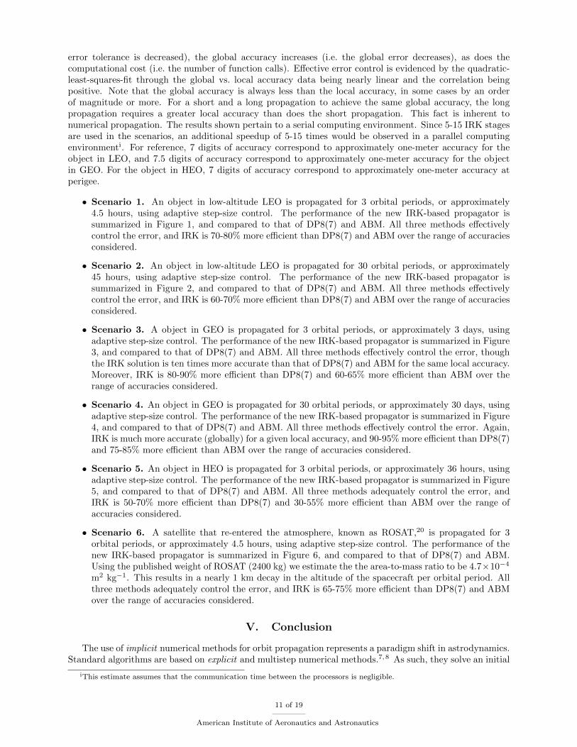
error tolerance is decreased), the global accuracy increases (i.e. the global error decreases), as does thecomputational cost (i.e. the number of function calls). Effective error control is evidenced by the quadratic-least-squares-fit through the global vs. local accuracy data being nearly linear and the correlation beingpositive. Note that the global accuracy is always less than the local accuracy, in some cases by an orderof magnitude or more. For a short and a long propagation to achieve the same global accuracy, the longpropagation requires a greater local accuracy than does the short propagation. This fact is inherent tonumerical propagation. The results shown pertain to a serial computing environment. Since 5-15 IRK stagesare used in the scenarios, an additional speedup of 5-15 times would be observed in a parallel computingenvironmenti. For reference, 7 digits of accuracy correspond to approximately one-meter accuracy for theobject in LEO, and 7.5 digits of accuracy correspond to approximately one-meter accuracy for the objectin GEO. For the object in HEO, 7 digits of accuracy correspond to approximately one-meter accuracy atperigee.

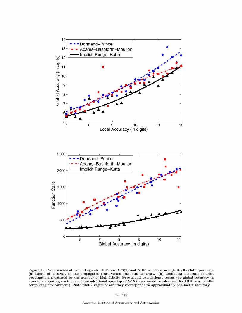
• Scenario 1. An object in low-altitude LEO is propagated for 3 orbital periods, or approximately4.5 hours, using adaptive step-size control. The performance of the new IRK-based propagator issummarized in Figure 1, and compared to that of DP8(7) and ABM. All three methods effectivelycontrol the error, and IRK is 70-80% more efficient than DP8(7) and ABM over the range of accuraciesconsidered.

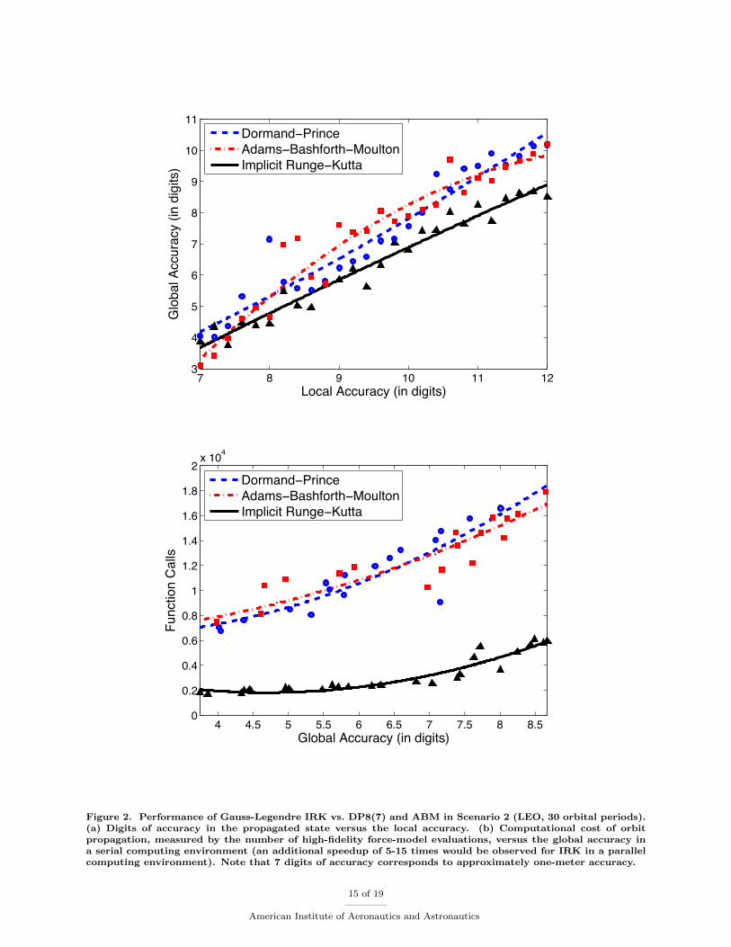
• Scenario 2. An object in low-altitude LEO is propagated for 30 orbital periods, or approximately45 hours, using adaptive step-size control. The performance of the new IRK-based propagator issummarized in Figure 2, and compared to that of DP8(7) and ABM. All three methods effectivelycontrol the error, and IRK is 60-70% more efficient than DP8(7) and ABM over the range of accuraciesconsidered.

• Scenario 3. A object in GEO is propagated for 3 orbital periods, or approximately 3 days, usingadaptive step-size control. The performance of the new IRK-based propagator is summarized in Figure3, and compared to that of DP8(7) and ABM. All three methods effectively control the error, thoughthe IRK solution is ten times more accurate than that of DP8(7) and ABM for the same local accuracy.Moreover, IRK is 80-90% more efficient than DP8(7) and 60-65% more efficient than ABM over therange of accuracies considered.

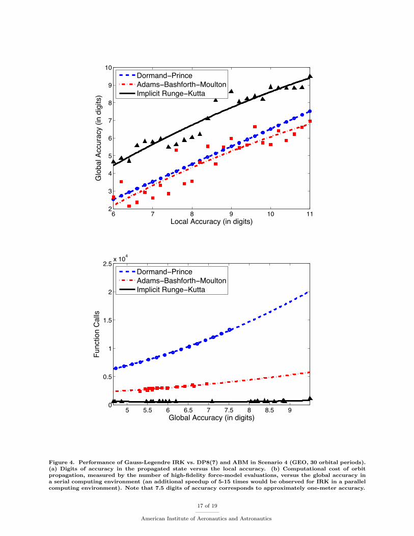
• Scenario 4. An object in GEO is propagated for 30 orbital periods, or approximately 30 days, usingadaptive step-size control. The performance of the new IRK-based propagator is summarized in Figure4, and compared to that of DP8(7) and ABM. All three methods effectively control the error. Again,IRK is much more accurate (globally) for a given local accuracy, and 90-95% more efficient than DP8(7)and 75-85% more efficient than ABM over the range of accuracies considered.

• Scenario 5. An object in HEO is propagated for 3 orbital periods, or approximately 36 hours, usingadaptive step-size control. The performance of the new IRK-based propagator is summarized in Figure5, and compared to that of DP8(7) and ABM. All three methods adequately control the error, andIRK is 50-70% more efficient than DP8(7) and 30-55% more efficient than ABM over the range ofaccuracies considered.

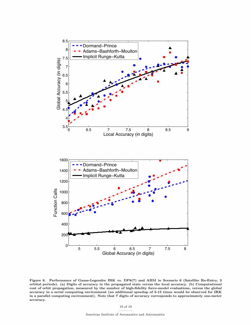
• Scenario 6. A satellite that re-entered the atmosphere, known as ROSAT,20 is propagated for 3orbital periods, or approximately 4.5 hours, using adaptive step-size control. The performance of thenew IRK-based propagator is summarized in Figure 6, and compared to that of DP8(7) and ABM.Using the published weight of ROSAT (2400 kg) we estimate the the area-to-mass ratio to be 4.7×10−4

m2 kg−1. This results in a nearly 1 km decay in the altitude of the spacecraft per orbital period. Allthree methods adequately control the error, and IRK is 65-75% more efficient than DP8(7) and ABMover the range of accuracies considered.

V. Conclusion

The use of implicit numerical methods for orbit propagation represents a paradigm shift in astrodynamics.Standard algorithms are based on explicit and multistep numerical methods.7,8 As such, they solve an initial

iThis estimate assumes that the communication time between the processors is negligible.

11 of 19


value problem by calculating the state of a system at a later time from the state of the system at the currenttime. Implicit numerical methods, on the other hand, solve an initial value problem by calculating the stateof a system at a later time from the state of the system at the current time, together with the state of thesystem at future times. Hence, an initial approximation for the solution is required, and the resulting systemof nonlinear equations must be solved iteratively.

What makes implicit Runge-Kutta (IRK) methods practical for orbit propagation is the availability ofanalytic and semi-analytic approximations to the solution that can be computed efficiently and used towarm-start the iterations, thereby lowering the computational cost of orbit propagation. IRK methodscan also be super-convergent, meaning that larger (and fewer) time steps can be taken than their explicitcounterparts. What is more, IRK methods are parallelizable. Explicit Runge-Kutta and multistep methodsare not. Even before parallelization, the new adaptive-step IRK-based orbital propagator is found to besignificantly more efficient in our test scenarios than adaptive-step explicit and multistep methods oftenused for orbital propagation, specifically, Dormand-Prince 8(7) and Adams-Bashforth-Moulton. Table 3 liststhe computational savings obtained in LEO (Scenarios 1–2), GEO (Scenarios 3–4), HEO (Scenario 5), andSatellite Re-Entry (Scenario 6) when medium- to high-accuracy propagations are performed.

Scenario 1 Scenario 2 Scenario 3 Scenario 4 Scenario 5 Scenario 6

LEO LEO GEO GEO HEO Re-Entry

SCE 70-80% 60-70% 60-65% 75-85% 30-55% 65-75%

PCE 94-99% 92-98% 92-98% 95-99% 86-97% 93-98%

Table 3. Summary of computational savings in a serial computing environment (SCE) or a parallel computingenvironment (PCE). The computational savings tend to increase as the accuracy of the propagation increases.

Not all orbital propagators estimate and control the truncation error by adapting the step size. Instead,fixed steps (in time or in an orbital anomaly) are taken.5,7, 8, 11 By taking fixed steps, one is assuming that(1) the nonlinearity in the underlying dynamics is approximately uniform over each step and (2) the stepsize yields a truncation error that is less than the error in the force models (but not too much less or elseunnecessary work is done to propagate the orbit). Unfortunately, one or both of these assumptions can beviolated. The first assumption breaks down when propagating low-altitude orbits, highly-elliptic orbits, ororbits over long enough time intervals. The second assumption requires a-priori knowledge of the truncationerror, which would need to be tabulated offline for a given set of force models and a large number of orbitpropagation scenarios. Our approach is to use an adaptive-step orbital propagator that uses online errorestimation and control wherein the acceptable level of truncation error can be tuned to the error intrinsic tothe force models. Therefore, the error estimates are more accurate, and the propagator does just the rightamount of work for a given propagation.

A large class of methods for propagating an orbital state and its uncertainty (e.g. the unscented Kalmanfilter,21,22 particle filters,23,24 Gaussian sum filters25–28) require the propagation of an ensemble of particles orstates through the nonlinear dynamics. Hence, orbit propagation is a prerequisite for uncertainty propagationusing these methods. In this paper, we demonstrated the use of implicit Runge-Kutta methods for accurateand efficient orbit propagation. In a companion paper,29 we demonstrate the use of implicit Runge-Kuttamethods for accurate and efficient uncertainty propagation.

Acknowledgments

The authors thank G. Beylkin and J. T. Horwood for helpful comments on earlier versions of this paper.This work was funded, in part, by a Phase II STTR from the Air Force Office of Scientific Research (FA9550-12-C-0034) and a grant from the Air Force Office of Scientific Research (FA9550-11-1-0248).

References

1Iserles, A., A First Course in the Numerical Analysis of Differential Equations, Cambridge University Press, Cambridge,UK, 2004.

2Butcher, J. C., Numerical Methods for Ordinary Differential Equations, John Wiley & Sons, West Sussex, England,2008.

12 of 19


3Hairer, E., Norsett, S. P., and Wanner, G., “Solving Ordinary Differential Equations I: Nonstiff Problems,” SpringerSeries in Computational Mathematics, Springer, 2nd ed., 2009.

4Hairer, E. and Wanner, G., “Solving Ordinary Differential Equations II: Stiff and Differential-Algebraic Problems,”Springer Series in Computational Mathematics, Springer, 2nd ed., 2010.

5Bradley, B. K., Jones, B. A., Beylkin, G., and Axelrad, P., “A new numerical integration technique in astrodynamics,”Proceedings of the 22nd Annual AAS/AIAA Spaceflight Mechanics Meeting, AAS 12-216, Charleston, SC, Jan. 30 - Feb. 22012, pp. 1–20.

6Beylkin, G. and Sandberg, K., “ODE Solvers Using Bandlimited Approximations,” arXiv:1208.3285v1 [math.NA] , 2012.7Berry, M. M. and Healy, L. M., “Implementation of Gauss-Jackson integration for orbit propagation,” Journal of the

Astronautical Sciences, Vol. 52, No. 3, 2004, pp. 331–357.8Montenbruck, O. and Gill, E., Satellite Orbits: Models, Methods, and Applications, Springer, Berlin, 2000.9Jones, B. A. and Anderson, R. L., “A survey of symplectic and collocation integration methods for orbit propagation,”

Proceedings of the 22nd Annual AAS/AIAA Spaceflight Mechanics Meeting, AAS 12-214, Charleston, SC, Jan. 30 - Feb. 22012, pp. 1–20.

10Vinti, J. P., “Orbital and Celestial Mechanics,” Progress in Astronautics and Aeronautics, edited by G. J. Der and N. L.Bonavito, Vol. 177, American Institute of Aeronautics and Astronautics, Cambridge, MA, 1998.

11Bai, X. and Junkins, J., “Modified Chebyshev-Picard iteration methods for orbit propagation,” J. Astronautical Sci.,Vol. 3, 2011, pp. 1–27.

12Berry, M. and Healy, L., “The generalized Sundman transformation for propagation of high-eccentricity elliptical orbits,”Proceedings of the 12th AAS/AIAA Space Flight Mechanics Meeting, San Antonio, TX, January 2002, pp. 1–20, Paper AAS-02-109.

13Kelley, C. T., “Iterative methods for linear and nonlinear equations,” Frontiers in Applied Mathematics, Vol. 16, SIAM,1995, pp. 1–180.

14Wright, K., “Some relationships between implicit Runge-Kutta, collocation and Lanczos methods and their stabilityproperties,” BIT , Vol. 10, 1970, pp. 217–227.

15Hulme, B. L., “One-step piecewise polynomial Galerkin methods for initial value problems,” Mathematics of Computation,Vol. 26, No. 118, 1972, pp. 415–426.

16Feagin, T. and Nacozy, P., “Matrix formulation of the Picard method for parallel computation,” Celestial Mechanics andDynamical Astronomy, Vol. 29, 1983, pp. 107–115.

17Fukushima, T., “Vector integration of the dynamical motions by the Picard-Chebyshev method,” The AstronomicalJournal , Vol. 113, 1997, pp. 2325–2328.

18Barrio, R., Palacios, M., and Elipe, A., “Chebyshev collocation methods for fast orbit determination,” Applied Mathe-matics and Computation, Vol. 99, 1999, pp. 195–207.

19Shampine, L. F., “Error estimation and control for ODEs,” J. Sci. Comp., Vol. 25, 2005, pp. 3–16.20Peat, C., “Heavens Above,” July 2012.21Julier, S. J. and Uhlmann, J. K., “Method and Apparatus for Fusing Signals with Partially Known Independent Error

Components,” U.S. Patent Number 6,829,568 B2, Issued on 7 December 2004.22Julier, S. J. and Uhlmann, J. K., “Unscented filtering and nonlinear estimation,” Proceedings of the IEEE , Vol. 92, 2004,

pp. 401–422.23A. Doucet, N.F. Freitas, N. G. and Smith, A., “Sequential Monte Carlo Methods in Practice,” Statistics for Engineering

and Information Sciences, Springer, 2001.24Ristic, B., Arulampalam, S., and Gordon, N., Beyond the Kalman Filter: Particle Filters for Tracking Applications,

Artech House, Boston, 2004.25Ito, K. and Xiong, K., “Gaussian filters for nonlinear filtering problems,” IEEE Transactions on Automatic Control ,

Vol. 45, No. 5, 2000, pp. 910–927.26Horwood, J. T. and Poore, A. B., “Adaptive Gaussian sum filters for space surveillance,” IEEE Transactions on Automatic

Control , Vol. 56, No. 8, 2011, pp. 1777–1790.27Horwood, J. T., Aragon, N. D., and Poore, A. B., “Gaussian sum filters for space surveillance: theory and simulations,”

Journal of Guidance, Control, and Dynamics, Vol. 34, No. 6, 2011, pp. 1839–1851.28DeMars, K. J., Jah, M. K., Cheng, Y., and Bishop, R. H., “Methods for splitting Gaussian distributions and applications

within the AEGIS filter,” Proceedings of the 22nd AAS/AIAA Space Flight Mechanics Meeting, Charleston, SC, February2012, Paper AAS-12-261.

29Aristoff, J. M., Horwood, J. T., and Poore, A. B., “Implicit Runge-Kutta methods for uncertainty propagation,” Pro-ceedings of the 2012 AMOS Conference, September 2012.

13 of 19


7 8 9 10 11 125

6

7

8

9

10

11

12

13

14

Local Accuracy (in digits)

Glo

bal A

ccur

acy

(in d

igits

)

Dormand−PrinceAdams−Bashforth−MoultonImplicit Runge−Kutta

6 7 8 9 10 110

500

1000

1500

2000

2500

Global Accuracy (in digits)

Func

tion

Cal

ls


Figure 1. Performance of Gauss-Legendre IRK vs. DP8(7) and ABM in Scenario 1 (LEO, 3 orbital periods).(a) Digits of accuracy in the propagated state versus the local accuracy. (b) Computational cost of orbitpropagation, measured by the number of high-fidelity force-model evaluations, versus the global accuracy ina serial computing environment (an additional speedup of 5-15 times would be observed for IRK in a parallelcomputing environment). Note that 7 digits of accuracy corresponds to approximately one-meter accuracy.

14 of 19


7 8 9 10 11 123

4

5

6

7

8

9

10

11


Glo

bal A

ccur

acy

(in d

igits

)


4 4.5 5 5.5 6 6.5 7 7.5 8 8.50

0.2

0.4

0.6

0.8

1

1.2

1.4

1.6

1.8

2x 104


Func

tion

Cal

ls


Figure 2. Performance of Gauss-Legendre IRK vs. DP8(7) and ABM in Scenario 2 (LEO, 30 orbital periods).(a) Digits of accuracy in the propagated state versus the local accuracy. (b) Computational cost of orbitpropagation, measured by the number of high-fidelity force-model evaluations, versus the global accuracy ina serial computing environment (an additional speedup of 5-15 times would be observed for IRK in a parallelcomputing environment). Note that 7 digits of accuracy corresponds to approximately one-meter accuracy.

15 of 19


6 7 8 9 10 113

4

5

6

7

8

9

10

11

12


Glo

bal A

ccur

acy

(in d

igits

)


6 6.5 7 7.5 8 8.5 9 9.5 10 10.50

200

400

600

800

1000

1200

1400

1600

1800

2000


Func

tion

Cal

ls


Figure 3. Performance of Gauss-Legendre IRK vs. DP8(7) and ABM in Scenario 3 (GEO, 3 orbital periods).(a) Digits of accuracy in the propagated state versus the local accuracy. (b) Computational cost of orbitpropagation, measured by the number of high-fidelity force-model evaluations, versus the global accuracy ina serial computing environment (an additional speedup of 5-15 times would be observed for IRK in a parallelcomputing environment). Note that 7.5 digits of accuracy corresponds to approximately one-meter accuracy.

16 of 19


6 7 8 9 10 112

3

4

5

6

7

8

9

10


Glo

bal A

ccur

acy

(in d

igits

)


5 5.5 6 6.5 7 7.5 8 8.5 90

0.5

1

1.5

2

2.5x 104


Func

tion

Cal

ls


Figure 4. Performance of Gauss-Legendre IRK vs. DP8(7) and ABM in Scenario 4 (GEO, 30 orbital periods).(a) Digits of accuracy in the propagated state versus the local accuracy. (b) Computational cost of orbitpropagation, measured by the number of high-fidelity force-model evaluations, versus the global accuracy ina serial computing environment (an additional speedup of 5-15 times would be observed for IRK in a parallelcomputing environment). Note that 7.5 digits of accuracy corresponds to approximately one-meter accuracy.

17 of 19


8 8.5 9 9.5 10 10.5 114

5

6

7

8

9

10

11


Glo

bal A

ccur

acy

(in d

igits

)


5 5.5 6 6.5 7 7.5 8 8.5 9 9.5500

1000

1500

2000

2500

3000

3500


Func

tion

Cal

ls


Figure 5. Performance of Gauss-Legendre IRK vs. DP8(7) and ABM in Scenario 5 (HEO, 3 orbital periods).(a) Digits of accuracy in the propagated state versus the local accuracy. (b) Computational cost of orbitpropagation, measured by the number of high-fidelity force-model evaluations, versus the global accuracy ina serial computing environment (an additional speedup of 5-15 times would be observed for IRK in a parallelcomputing environment). Note that 7.5 digits of accuracy corresponds to approximately one-meter accuracyat perigee.

18 of 19


6 6.5 7 7.5 8 8.5 93.5

4

4.5

5

5.5

6

6.5

7

7.5

8

8.5


Glo

bal A

ccur

acy

(in d

igits

)


5 5.5 6 6.5 7 7.5 80

200

400

600

800

1000

1200

1400

1600


Func

tion

Cal

ls


Figure 6. Performance of Gauss-Legendre IRK vs. DP8(7) and ABM in Scenario 6 (Satellite Re-Entry, 3orbital periods). (a) Digits of accuracy in the propagated state versus the local accuracy. (b) Computationalcost of orbit propagation, measured by the number of high-fidelity force-model evaluations, versus the globalaccuracy in a serial computing environment (an additional speedup of 5-15 times would be observed for IRKin a parallel computing environment). Note that 7 digits of accuracy corresponds to approximately one-meteraccuracy.

19 of 19


implicit runge-kutta methods for orbit propagation...implicit runge-kutta methods for orbit...

Documents