implicit perceptual learning during passive listening o f...
TRANSCRIPT

Implicit perceptual learning during passive
listening of sound sequences: an ECoG study
Raphaëlle Bertrand-Lalo
Supervised by
Jérémie Mattout and Gerwin Schalk
Co-supervised by
Françoise Lecaignard and Peter Brunner
Master of cognitive neuroscience, ENS
(~12271 words )
September, 2017

Table of contents
Abstract 4
Contributions 5
Distinctiveness Statement 6
Introduction 7 Scientific Background 7
Perception and learning 8 Electrophysiological brain signals 8 A predictive coding perspective 11 Open questions 12
An original EEG/MEG study 13 Experimental paradigm 13 Main results 14
The current ECoG study 15 Motivations 116 Related recent ECoG studies 16 Outline of the report 18
Method 19 Participants 20 Experimental design 20 ECoG recordings 22 Data preprocessing 22 Montage reference 23 ERP analysis 24 Spectral analysis 25 Computational modeling (ERP analysis) 26
29
Results 30 ERP analysis 31
Responsive sensors 31 ERP sensor-level 34 Computational modelling 36
Spectral analysis 40
1

Responsive sensors 40 Alpha 41 Broadband gamma 45
47
Discussion 48 ERP analysis 49 Spectral analysis 49
ECoG limitations 52 Number of subjects 52
Supplementary material: 53 ECoG clinical and research procedure 53 Patient rejection 54 Detailed results from statistical analysis 56
59
Bibliography 60
2

Abstract
Auditory oddball paradigms have been widely used for almost four decades, to study human
perception and perceptual learning. Despite a huge amount of data, these processes remain partly
unknown but the oddball paradigm is still very much used, namely because of the recent
computational theories that have associated electrophysiological responses to oddball stimuli with a
measure of surprise or prediction error. This is the case for the well-known Mismatch Negativity
(MMN) component.
The MMN is traditionally measured with Electroencephalography (EEG). It is acknowledged as a
marker of automated or implicit perceptual learning, not only in the auditory domain but also other
sensory modalities. It reflects the processing of sequences of stimuli and is one of the most robust
marker of the updated predictions computed by the brain. It is thus a valuable marker to study
predictive coding by the brain.
Moreover, the MMN has been shown to be altered in several neurological and psychiatric conditions,
which makes it also valuable to study brain dysfunctions. What remain unknown though are the
precise computational processes at play during auditory sequence processing and their
neurophysiological correlates, including but also beyond the MMN.
Recent experimental studies implementing new tone sequences have revealed the structure in the
trial by trial variations of electrophysiological responses. These variations at various post-stimulus
latencies, suggest that a fronto-temporal cortical hierarchy support the perception of sound
sequences up to the level of contextual regularities.
In the aim of finely characterizing this cortical network, both at the algorithmic and
electrophysiological levels, my project consisted in combining for the first time, these new auditory
sequences with the high spatial, temporal and frequency resolution of Electrocorticographic (EcoG)
recordings of implanted epileptic patients.
Three patients have been recorded so far. This report describes in details the analysis of the first
patient’s data.
Three main analysis were conducted:
1. An event-related potential analysis in order to relate ECoG findings with known
EEG findings, namely identifying the spatio-temporal signature of mismatch
responses as well as the effect of sequence predictability.
3

2. A trial-by-trial computational analysis of the above (low frequency) responses in
order to reveal the associated computational learning processes.
3. An analysis of oscillatory and high frequency activities in the alpha and broad
gamma bands.
We observed a mismatch response at the latency of the MMN which was modulated by predictability
as expected: i.e. its amplitude was reduced as the sequence was more predictable. Moreover, the
computational analysis of trial-by–trial responses revealed that mismatch responses over time are
not simply binary (different for the standard and the deviant tone) but reflects perceptual learning in
the sense that they correlate with surprise as predicted by an approximate Bayesian learning model.
Finally, we observed alpha suppression as well as an increase in broadband gamma after a deviant
tone. An effect that was reduced with predictability.
Keeping in mind that these findings come from one subject only, we discuss the consistency of these
results with other findings and existing theories in the literature. We conclude this report with some
perspective of this work.
Contributions
While the desire to study human perception and learning was mine, many helped in the literature
review, experimental design, and data analysis.
Claire Sergent helped me pave the way by sending me relevant literature that she believed would be
helpful in my research.
Françoise Lecaignard, Anne Caclin and Jérémie Mattout have been of a precious help from the very
beginning in sharing with me the oddball paradigm that they designed and introduced me to the
great literature dealing with mismatch negativity and computational neuroscience. Françoise
trained me to use the Elan Software and with the contribution of Emmanuel Maby and Aurelie
Bidet-Caulet, she supervised me at each step of the signal processing.
4

The ECoG data were collected with Lawrence Crowther, Ladan Moheimanian, Peter Brunner and
James Swift. The 3D cortical brain models and the electrodes’ coordinates were determined by Peter
Brunner and Lawrence Crowther using Freesurfer, SPM8 and custom MATLAB scripts.
I set up the experiment, with the help of Peter Brunner; he checked and reviewed all my studies
before running them online. Peter then introduced me to ECoG signals from scratch, aided me in my
analysis and gave me critical feedback about how to perform the right statistics.
Jérémie Mattout and Gerwin Schalk both aided me in identifying and clarifying my specific research
questions.
I made the theoretical interpretations and wrote the thesis. Jérémie Mattout, Françoise Lecaignard,
Peter Brunner and Gerwin Schalk gave me precious feedback on this work, including theoretical
notes, style as well as presentation and analysis notes.
I am very grateful for all their contributions.
Distinctiveness Statement
The originality of our approach lies in the combination of:
- A recently proposed auditory sequence that carefully manipulates sound
predictability;
- Computational models of perceptual learning that can be tested against
trial-by-trial variations of electrophysiological responses;
- EcoG recordings in epileptic patients in order to benefit from high spatial,
temporal and frequency resolution, to characterize the functional anatomy of
implicit perceptual learning within the auditory cortical hierarchy.
5

Introduction
A) Scientific Background
a) Perception and learning
i) Perceiving sequences
A pixel is of little interest if it is not considered as part of a picture. Similarly, a sound is only
meaningful as part of a scene. Humans are confronted with a tremendous amount of information
that needs to be processed as part of a whole, as part of a broader picture, a context. Hence,
segregation of information is inherent to any cognitive process. We perform sequencing of sensory
inputs every day to make sense: speech or music sounds, actions…
This process involves being able to extract and store the right information at different levels of
details. Several neural mechanisms have so far been proposed and reviewed in1.
ii) Implicit learning in the auditory domain
You don’t have to be Victor Hugo nor Wolfgang Mozart to sense that “This is not right”/”That sounds
wrong” when a non-native speaker utters a grammatical mistake in your language, or when a
musician breaks the rules of harmony. Indeed, human learners are highly sensitive to the
hierarchical structures in their environment and are able to extract the rules underlying these
structures, without intention and awareness. First introduced by Reber (1967) in a seminal paper on
artificial grammar learning, the term “implicit learning” refers to the way people acquire the
regularities of their environment, without any effort. A body of evidence suggests that implicit
learning governs language 2,3 and music 4 acquisition and perception.
My project aimed at better characterizing the mental processes and physiological mechanisms
underlying implicit perceptual learning of structured sound sequences.
6

iii) The experimental paradigms to study the implicit learning of
perceptual sequences
Perceptual sequences
To investigate how the brain deals with sequences of sounds, one typically uses an oddball paradigm,
i.e. one presents a sequence of identical and frequent stimuli ( the standards), occasionally interrupted
by a different rare sound ( a deviant).
The stimuli can be of different types: tactile 5, visual6, auditory7. And the dimension along which they
differ may be frequency, intensity, duration… Note that another way of eliciting a mismatch response
is simply to omit the stimulus8, as the timing of the sequence is also important and could be predicted
by the brain.
In order to tackle the learning process underpinning the perception of sequences, the experimental
design may further manipulate the temporal or statistical regularity of the sequence. For instance, the
occurrence of deviant sounds may follow a deterministic (i.e., highly predictable) pattern or a random
(i.e., less predictable) one.
Implicit presentation
In order, to investigate the implicit extraction of the environmental regularities, the attention of the
subject must be diverted away from the sequence of stimuli.
To this end, the subject or patient is given another task, such as watching a movie or responding to
asynchronous stimuli in another sensory modality.
Such paradigms are referred to as passive as the sequence of interest is thus passively perceived. It
does not require any behavioral response or report. It does not require the voluntary focus of
attention.
b) Electrophysiological brain signals
Electrophysiological brain signals can be analyzed either in the time domain or in the spectral
domain.
In the time domain, we refer to evoked related potential (ERP) as averaged responses that are
time-locked to stimulus presentation.
In the spectral domain, we refer to oscillations or high frequency activities that represent synchronized activity of neuronal populations. By convention they are divided into frequency bands like: delta (δ, <4
7

Hz); theta (θ, 4–7 Hz); alpha (α, 8–12 Hz); beta (β, 13–29 Hz); low gamma (Lγ, 30-60Hz); broadband gamma (Hγ, >60Hz). Here, we focus our analysis on ERPs, alpha and broadband gamma activities.
i) Mismatch Negativity
The Mismatch Negativity (MMN) is an evoked related potential (ERP) elicited by the violation of a
rule, established by a sequence of sensory stimuli. First discovered by Näätänen9 , it is widely accepted
that the MMN reflects the brain’s ability to detect a change in the environment10,11. Since then, many
mechanisms have been proposed to explain the MMN, such as the “stimulus adaptation” and the “model
adjustment ” hypothesis (for a review, see 7). Either way, the MMN is widely recognized as a measure for
surprise.
Mismatch Negativity has been associated to “primitive intelligence”12. It is worth noting that this
response cannot be refrained and does not need any attention from the subject. In fact, the MMN was
also found in babies13, in coma14, during sleep 15, or under anesthesia 16 .
Encephalographic recordings showed that the MMN typically peaks at about 100-250 ms after the
stimulus onset (reviewed in17). However, the mechanisms underlying the generation of the MMN
remain unclear. Though, recent studies5,18,19 using dynamical causal modelling (DCM) of evoked
responses20 pertain to a bilateral fronto-temporal cortical network, hierarchically organized. The
MMN would result from the interplay between those regions, through forward and backward message
passing.
ii) Alpha oscillations
Alpha oscillations reflect cortical excitability
Alpha oscillations are associated with a rhythmic inhibition of cortical processing21 . In other words,
alpha power increases in the areas of the brain that are not involved in the current task (e.g over
occipital cortex when a subject closes the eyes22) and decreases elsewhere (e.g. over auditory cortex
when a subject listens to sounds23,24 ; or over the contralateral motor cortex during voluntary
movement 25–27.). It was further found that decreases of alpha power reflects the excitability of the
cortex 28–30) and enhances the efficacy with which information is processed 31–35. For example, reduced
alpha power over the occipital cortex promotes the perception of subtle visual stimuli29,36 and is
8

observed in anticipation of an upcoming stimulus31–3537,38. Indeed, one way to convey the information
from one area of the brain to another is to inhibit the irrelevant pathways and this inhibition could be
mediated by oscillatory activity in the alpha band39,40 .
Alpha oscillations in the auditory system
Auditory cortical areas being spatially more confined than visual or sensorimotor ones, may explain
why it appears more difficult to reveal alpha rhythms in the auditory cortex with scalp recordings.
However, there is also an auditory alpha-like rhythm independent of visual and motor generators.
The feasibility of recording alpha-like dynamics from auditory cortex is reviewed in41. Authors report
that there is indeed the equivalent of a resting state in the auditory system whose perturbation (e.g.
by the presentation of a sound) yields a momentary suppression of alpha power.
Alpha oscillations and evoked responses
Post-stimulus alpha and other low frequency oscillations may be linked to evoked related potentials
(ERPs). Three main theories have been proposed to explain ERPs (for a review see:42): additivity,
phase-resetting and baseline-shift. Additivity and phase reset theories offer an explanation for
exogenous early components. The former suggests that the stimulus itself involves a time-locked
response superimposing to the background activity in each trial, whereas the latter suggests that the
phase of ongoing oscillations get aligned to the stimulus. In both case, averaging over trials leads to a
time-locked component that differs from the baseline. The baseline-shift theory relies upon the
asymmetry in the amplitude of the oscillations, such that the peaks of the oscillations are more strongly modulated than the troughs, leading to a depression (or increase) in the oscillatory activity in response to a stimulus.
Additional studies have shown that background alpha in particular predicts the latency and the
amplitude of ERP components such as the P1-N143,44 , and the P345.
Alpha oscillations and cognitive skills
Finally, regarding the functional interpretation of alpha activity, it has been shown to modulate or
correlate with perception, attention and memory46,47
9

iii) Broadband gamma
Increases in broadband gamma power provide a measure of the local average firing rate of neuronal
populations, as demonstrated by 48 using local field potentials (LFP).
Moreover, broadband gamma power has been shown to be tightly correlated with the cortical activity
of neuronal populations involved in a task. For example, broadband gamma power increases in motor
areas during motor movements 49–51 , in areas of speech processing during speech perception 23,52 , in
auditory cortex during music perception 53,54 and auditory attention 55,56, in sensorimotor, prefrontal
and visual areas during visual spatial attention 57,58, and in speech production areas during overt
speech 59 or imagined speech 60.
An overview of auditory broadband gamma responses and the methods to study them is provided in
tutorial 61.
c) A predictive coding perspective
Predictive coding has been proposed to model the processing of new information in the brain based
on the assumption that the brain adapts to its environment in a fashion that is closed to optimal
described by bayesian statistics.
Bayesian Brain hypothesis states that the brain constantly updates an internal model of the
environment which enables to predict the sensory environment and weighs these predictions
depending on how trusty they are. The key computational components are:
- The prediction (Pd);
- The prediction error (PE), ie. the difference between the prediction and the
observation;
- The precision weight (PW), which signals when it is worth updating the internal
model;
- The precision-weighted-prediction-error (PWPE);
Friston 62 proposed that the ERPs encode for PWPE in the brain, hence that the MMN could be
understood as a PWPE. Predictive coding reconciles the adaptation and the model adjustment
hypothesis7. to explain mismatch responses and the MMN in particular and was used in 5,18,63 to study
10

how brain activity (that reflects the processing of the sequences of sounds) is modulated by the
experimental manipulations.
In a predictive coding scheme, mismatch responses can be measured at each level of a cortical
hierarchy is the result of a bottom-up message passing of prediction errors and a top-down message
passing of predictions. Strong efforts to control the biological plausibility of a (cortical)
implementation of a predictive coding scheme have been done.
Recent studies (reviewed in 64) suggest that differences in neuronal dynamics of superficial and deep
layers could explain this two-ways flow of information. Practically speaking, superficial layers in
charge of forward messages (PE or PWPE) , while deep layers in charge of backward messages (Pd,
PW). In addition, superficial layers tend to synchronize in high frequencies (gamma) and deep layers
would rather express in lower frequencies (alpha, beta). Accordingly, prediction errors (PE) would be
conveyed by broadband activity, while precisions (PW) and predictions (Pd) would be reflected by
alpha and beta activities 65 .
Such model provides precise predictions: the higher the PWPE, the greater the increase in high
frequency activity, while the more relevant the incoming PE, the higher the PW, hence the lower the
alpha activity.
d) Open questions
Studies using scalp recordings suggest that the MMN has interacting generators in the temporal and
frontal lobes 7. The distinct contribution of each part of this network, especially the prefrontal one,
could worth further investigations though. Studies of patients with prefrontal lesions suggest a
critical role of the prefrontal cortex on contextual processing 66 and working memory 67. Yet, previous
intracranial recordings using a mismatch protocol showed a frontal participation in the MMN
generation in some patients, but not all. For example, 68,69 investigated 29 patients and found an
intracranial MMN in the superior temporal lobe for 13 patients, in the inferior frontal gyrus for 2
patients and in the frontal interhemispheric fissure for only 1 patient. Hence, there is work needed in
refining the spatio-temporal characteristics of the mismatch responses measured directly from the
surface of the brain.
11

Furthermore, the high level of noise often restricts the analysis to low frequency70 and only a few
research studies have investigated the high frequency correlates of auditory oddball sequence
processing. Nevertheless, there are recent evidence in favor of crucial high frequency contributions,
shedding light on the involved levels of the cortical hierarchy 71 and the functional role of oscillations 72.
This summarized status of knowledge calls for a refined description of the functional anatomy of
implicit auditory perceptual learning, namely through the characterization in space, time and
frequency of mismatch responses and their contextual modulations.
B) An original EEG/MEG study
My project used the same experimental paradigm as the one proposed in a recent study by Françoise
Lecaignard and colleagues from the Lyon Neuroscience Research Center (CRNL). They used
non-invasive recordings (simultaneous electroencephalography (EEG) and magnetoencephalography
(MEG)) during a passive oddball auditory paradigm in which the predictability of the sound
sequences were manipulated so as to test predictive coding hypothesis in auditory perception to
characterize the learning behind deviance processing. Precisely, the PWPE decreases with
predictability and if MMN is indeed a PWPE (Friston), then MMN should decrease with
predictability.
a) Experimental paradigm
This coupled EEG-MEG study was performed on 27 healthy subjects, among which 22 were retained
for post-experimental debriefing. They used an auditory oddball paradigm with a frequency deviant.
The probability for a deviant sound to occur was set to 17% in all sequences. However, in the
predictable sequences (PF, where ‘P’ states for Predictable and ‘F’ for the type of deviance used, ie.
Frequency), the number of standards preceding a deviant was incremented regularly from 2 to 8,
whereas in the unpredictable sequences (UF, where ‘U’ states for Unpredictable), there was no such
ordered pattern.
12

b) Main results
i) Effect of predictability on ERPs
In a first stage, Lecaignard et al. showed that the Mismatch Negativity (MMN) was shaped by
predictability, such that the more predictable the deviant stimulus is, the smaller the elicited
mismatch response.19 (FIG.1 ). This effect was interpreted as a signature of the learning of the
structure of the sequence. Importantly, the subjects were watching a movie, making the experiment
a passive listening task. The observed learning was implicit. A debriefing of the subjects after the
recording confirmed that they did not notice a difference between sequences.
FIGURE 1 | Findings of Lecaignard et al. (2015). The grand-average ERPs (N = 22 subjects) measured in EEG, elicited by difference responses at electrode Fz in bandwidth 2–45 Hz for condition UF (red) and PF (green). Shaded areas display the windows of statistical significance.
ii) Source reconstruction
In a second stage, EEG and MEG data were fused and inverted so as to localize the cortical network
of the MMN. For each subject and each trial, activity was reconstructed in each source of this
fronto-temporal network. This activity was then used to compare alternative computational models
of perception (see below).
iii) Underlying computational processes
In a third stage, Lecaignard et al. tested different hypotheses of how such a learning of the
regularities between the sounds had been performed by these cortical sources. Using computational
learning models 5 and dynamic causal models of evoked responses 20,73, they showed that the MMN
does not reflect a simple deviance detection mechanism, but rather a (precision-weighted) prediction
error (PWPE) which is shaped by the informational content of the auditory. When moving from an
13

unpredictable to a predictable sound sequence, prediction error was found to be reduced while its
precision increased 74 .
C) The current ECoG study
My project aimed at trying to refine the above results and answer the new questions raised by this
initial EEG-MEG study, but which required a higher spatial and frequency resolution than the one
provided by non-invasive recordings. Therefore, we initiated a fruitful collaboration between the
Center for Medical Science in Albany, USA and the Lyon Neuroscience Research Center in France.
This collaboration provided me with the needed access to intra-cortical data (EcoG measures in
epileptic patients implanted for neurosurgery planning) and the rich complementary expertise in
human electrophysiology, signal processing and computational neurosciences.
Importantly, the experimental design of our task has a twofold advantage which makes it particularly
appropriate for testing with implanted epileptic patients:
- It is a completely passive, hence very easy to perform;
- It involves the auditory system, a fronto-temporal network that is often covered (at least
partially) by EcoG implants since most patients suffer from temporal epilepsy.
a) Motivations
i) Taking advantage of the fine spatial resolution
The results obtained by Lecaignard et al. identified the activation of a bilateral fronto-temporal
cortical network which was reconstructed by combining spatial information from both EEG and
MEG, at the group level. Computational modelling succeeded in revealing learning within each
source at the MMN latency. However, no spatio-temporal pattern could be found. For instance one
could have expected that the frontal part to be more sensitive to slowly evolving features in the
environment (typically the context and what makes a sequence more or less predictable), whereas the
lower temporal part of the hierarchy would be more sensitive to short scale changes 62. Such absence
of findings may be due to the limits of inverse modelling, that we hopefully don’t have to face using
ECoG recordings.
14

Since EcoG combines high temporal and spatial resolutions, we hoped to shed light on this time
resolved specialization within the hierarchy.
This motivation was clearly defining the successive steps of our investigation:
(1) To identify and confirm the hierarchical network underlying the processing of
sound sequences (change detection and its more or less predictable context);
(2) To assess the functional role of the different levels of the cortical hierarchy, using
computational modelling in combination with the high temporal resolution of
electrophysiological recordings.
ii) Taking advantage of the larger frequency range
In addition, ECoG data provide the opportunity to study cortical responses in higher frequencies,
with a much higher signal to noise ratio, allowing for single subject level analysis. Namely, using the
same experimental paradigm, we could test the modulation of different cortical rhythms with
predictability and test their computational implication in the learning process. Practically speaking,
this allows us to test the precise hypothesis cited above: alpha codes for precision and broadband
gamma for PE/PWPE.
Our aim was first to test whether our experimental manipulations, either local (mismatch) or global
(change in predictability) would modulate alpha and/or gamma activity. If so, informed by
computational models of perceptual learning, we would thus be in a position to specific hypothesis
about the functional role of these oscillatory and broad band activities.
b) Related recent ECoG studies
i) Physiological findings using ECoG and auditory/visual oddball
Using intracranial recordings, studies could confirm scalp findings, by showing that in the temporal
gyrus (TG) and frontal gyrus (FG), there was indeed a significant difference between the responses
evoked by the standard and the deviant stimuli, respectively, at the MMN latency (100-200 msec) 71,75–78
.
Additionally, time-frequency analyses showed significant broadband gamma responses to auditory
stimuli 71,75,77,79–81 followed by a decrease in alpha power 23. Precisely, these studies report evidence for an
15

early stronger increase of broadband gamma power in response to deviant compared to standard tones, and a correlation between the amplitude of broadband gamma power (at around 50–200 ms), followed by an α power decrease (at around 200-450ms). This is consistent with an other study of Knight and colleagues, that showed a coupling between
broadband gamma amplitude and alpha troughs, which is stronger in the visual cortical regions
during visual task 81
These findings have been interpreted as coupling between frequencies and a signature of reciprocal
but asymmetrical message passing within the hierarchy, in line with the structural asymmetry
between feedforward and backward pathways. The former would thus be facilitated by broadband
gamma, while the latter would convey information carried by alpha decrease.
ii) Predictive coding related findings
Two recent EcoG studies provided evidence for a predictive coding based interpretation of
perception of sound sequences.
In 72 (2016) , the focus was on the distinct role of different spectral activities in the implicit learning
process. This study involved three epileptic patients implanted with contact depth electrodes along
the axis of the axis of Heschl’s gyrus. Patients were presented with series of sounds of different
frequencies. The authors used an original design where sounds were generated by a hidden
hierarchical generative model. Standard and deviant sounds were both drawn from two different
gaussian distributions centered on their respective fundamental frequency. The mean and standard
deviations of those distributions could theoretically be inferred through prolonged perception. This
implicit process was modelled by a Bayesian learning model whose computed quantities could then
be correlated with the dynamics of local field potentials over trials, in various frequency bands.
The author could show a correlation between gamma band power fluctuations (>30 Hz) and
prediction error (PE) , beta band activity (12-30 Hz) and prediction (Pd) , and between alpha band
activity (8-12 Hz) and the precision of prediction error (PW).
In 71 (2016), the focus was on the role of the different cortical areas in the implicit learning process.
This ECoG study used a paradigm relatively close to ours. Five epileptic patients were presented with
an auditory oddball paradigm in which the standard and deviant tones differed by their frequency
16

(500 and 550 Hz respectively). The deviant sound occurred with a constant probability of 0.2 but was
presented either regularly (i.e., after every five standards) or randomly. Hence, although the
occurrence of the deviant followed the same probability, its position is fully predictable in the first
condition only. The authors focused on ERP and broadband gamma. They found: 1) a
deviance-related effect in temporal and frontal areas in both frequency range, with an earlier latency
for broadband gamma than ERP; 2) A predictability-related effect in frontal areas in broadband
gamma but not ERP.
To conclude, these promising findings, in keeping with predictive coding assumptions, highlight the
need for trial-wise modelling to go beyond speculation and test the dynamics of learning,
questioning both its psychological and physiological underpinnings.
c) Outline of the report
The first part of my work aimed at characterizing the (EcoG equivalent of the) Mismatch Negativity
and to investigate other deviance related responses, in a physiologically motivated approach.
Specifically, I focused on three signal features: 1) MMN as a measure for cortical mismatch, 2) Alpha
power (8-12 Hz) as a measure of cortical excitability; and 3) Broadband gamma power (70-170 Hz) as a
measure of population level activity.
The second part of my work aimed at analyzing the modulation of cortical activity by predictability,
through the quantification that is at quantifying of the effect of the sequence statistical structure
onto the deviance measures.
The third part of my work aimed at modelling the above effects at the single trial level, using
psychophysiological computational models of implicit learning. Precisely, following Lecaignard et
al.’s rationale, we hypothesize that the brain is an approximate Bayesian observer with an internal
model of how the sequence of sounds is generated. Such an observer uses this model online to update
its parameters and optimize its predictions about the auditory stimuli to come 82 .
17

This report is organized as follow:
The first part of this report aimed at providing a general context for this project. We provided the
necessary scientific background of this project and a brief overview of the main associated findings
in the field of perception, neurophysiology and computational neuroscience. Then, we presented the
original EEG/MEG study behind the designing of this project and finally, we described the
motivations and objectives of the current ECoG study.
In the second part, we will present the methodology. First, we present the experimental framework
(participant, experimental design, recordings). Then, we describe the signal processing strategy
(preprocessing, referencing), as well as the feature extraction and the statistical analysis (for ERP
and Oscillatory activity separately). Finally, we introduce the computational modelling approach.
Therefore, we underly the key elements of Bayesian learning, we present our different models, and
the methodology used to confront them to the data.
In the third part, we report the results obtained with the first ECoG subject. We first present the
findings from the ERP analysis, including the analysis of averaged responses and the trial-by-trial
modeling approach. We then move on to the spectral analysis restricted to the analysis of averaged
responses.
In the fourth and last part, we interpret and describe the significance of our findings.
Method
The present study was conducted with electrocorticography (ECoG) recordings of neurosurgical
epileptic patients at the Albany Medical Center (Albany, New York). It rests on the oddball paradigm
previously used in Lecaignard et al. (2015) that comprises predictable and unpredictable tone
sequences (with regard to deviant occurrence). We performed two separate analyses to assess the
perceptual learning at play during passive auditory processing: the first one was based on
event-related potentials (ERPs, 2-20 Hz bandwidth) and will be referred to as the ERP analysis. The
second one pertains to the oscillatory activity in the alpha band (8-12 Hz) and broad-gamma band
(70-170 Hz) and will be referred to as the spectral analysis. For each analysis, we conducted in a first
step a typical comparison between conditions based on averaged responses across trials. And we plan
18

to perform in a second step a trial-by-trial computational modeling approach to capture the
dynamics of learning (if any) over the course of the experiment. During my internship, it could be
achieved for the ERP part only. For each analysis and for each approach, we tested an effect of
deviance (standard vs. deviant) and an effect of predictability (predictable vs. unpredictable).
A. Participants
During my internship, four subjects (or patients) were included in the study. They underwent
temporal placement of electrocorticographic grids over frontal, parietal and temporal cortices. All
patients provided written informed consent prior to this study, which was approved by the
Institutional Review Board of Albany Medical College and the Human Research Protections. In the
present manuscript, we report findings from one patient (referred to as Su78, male). Two patients
had to be excluded (one with data highly contaminated with epileptic activity, and the other one with
unresponsive data with regard to the auditory stimuli; more details can be found in the
Supplementary Materials). The fourth patient was recorded at the very end of my internship and is
currently being processed.
B. Experimental design
To insure that the auditory listening remains passive, the subject was awake during the experiment
and watched a silent movie with subtitles. He was instructed to ignore the sounds. A short
debriefing at the end of the experiment aimed at checking that the subject did not notice the
difference between the predictable and unpredictable conditions. (eg. “ Were you concentrating on
the movie ?”, “Did you pay attention to the sounds ?”, ‘Did you notice any pattern in the sequences ?”).
The subject listened to stimuli consisting of 80-ms-long (with 5 ms rise/fall) harmonic sounds
differing in their fundamental frequency (500 Hz; 550 Hz). The stimulus onset asynchrony (SOA) was
fixed to 600 ms. The stimuli were delivered using BCI-2000 software (Schalk et al., IEEE Trans
Biomed Eng, 2004 , http://www.bci2000.org ) and presented with loudspeakers placed near the
subject’s bed at a low but audible level.
The sounds were presented either in a predictable (i.e., structured) or unpredictable (i.e.,
pseudo-random) sequence with the same deviant probability (p = 0.17).
19

In the predictable condition (referred to as PF), the deviants are presented in a deterministic periodic
pattern. In contrast, in the unpredictable condition (referred to as UF), the deviants are presented
pseudo-randomly. The rule was based on the number of standards that precedes the deviant. As
depicted in FIG.2 the number of successive identical tones preceding a change was incremented and
decremented progressively for PF, whereas it was pseudo-randomly chosen in the unpredictable
condition. As in Lecaignard et al. 2015 , let us define a “chunk with n standards” as a sequence of n
repetitive tones ending by a different one. Hence, both PF and UF sequences can be seen as
successive n chunks, with different length (n ranging from 2 to 8). The chunks are presented within
cycles of seven incrementing chunks and seven decrementing chunks. In the UF sequences, the order
of the chunk are shuffled, in a pseudo-random way, so that there can be neither successive
incrementation nor decrementation, or consecutive chunks with n standards.
Importantly, such rule allows the same history of deviants in both condition (unlike 71. Hence, our
predictability manipulation consists in a contextual manipulation of exactly the same local rule.
Each sequence type (PF ; UF) was delivered twice in separate 7 min long blocks, resulting in 224
deviants in each condition. To ensure an optimal control for undesirable effects of specific acoustic
properties, we switch the role of the tones in subsequent runs. Namely, the sound frequency used as
the standard in the one block becomes the deviant in the other (reverse) block.
FIGURE 2 | Experimental design. Scheme of a complete cycle in predictable (left) and unpredictable (right) condition. Chunk are sorted by their size in the predictable conditions (ascending, descending order), and are shuffled in the unpredictable condition. Above, the serie of chunk from the shaded area is depicted for each condition. Circles symbolize single tones (standard and deviant). Sound duration is 80 ms with stimulus onset asynchrony (SOA) set to 600 ms.
20
C. ECoG recordings
a) Data acquisition
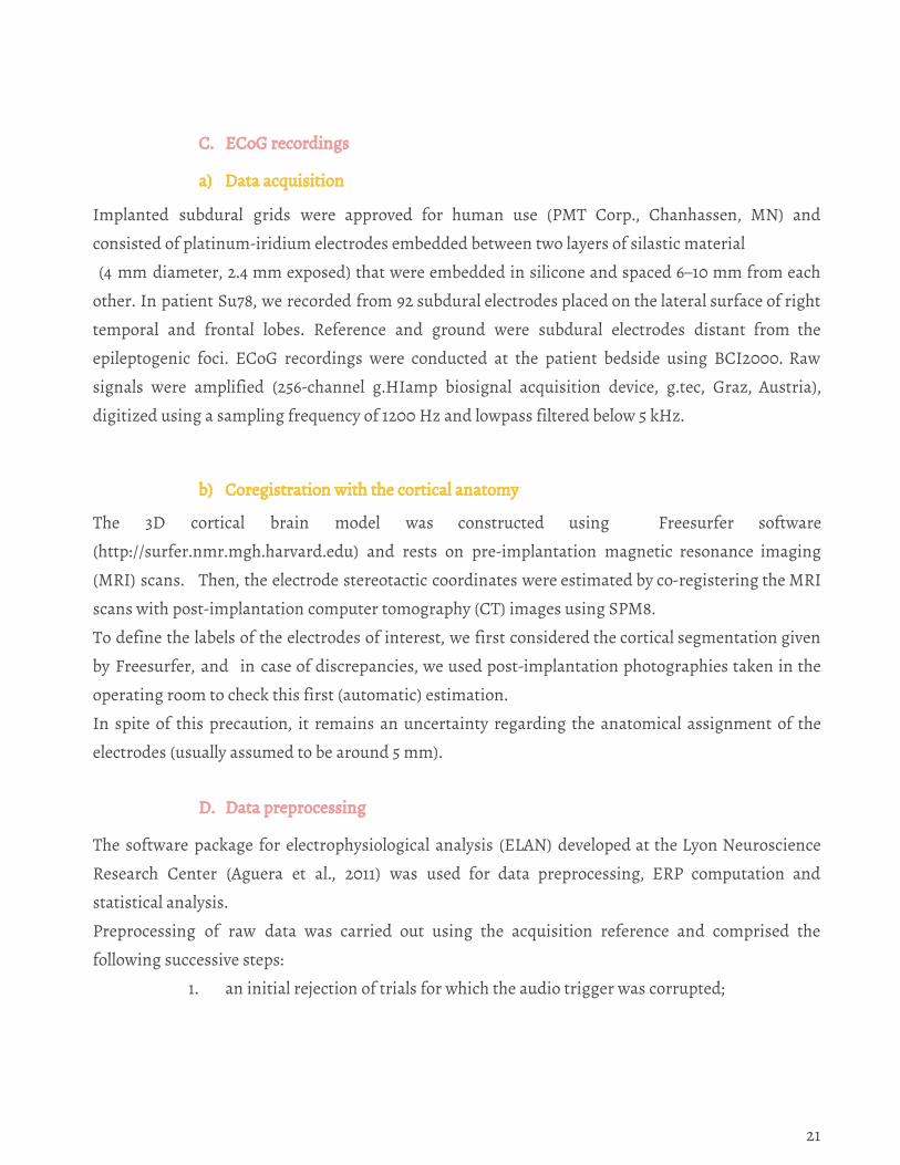
Implanted subdural grids were approved for human use (PMT Corp., Chanhassen, MN) and
consisted of platinum-iridium electrodes embedded between two layers of silastic material
(4 mm diameter, 2.4 mm exposed) that were embedded in silicone and spaced 6–10 mm from each
other. In patient Su78, we recorded from 92 subdural electrodes placed on the lateral surface of right
temporal and frontal lobes. Reference and ground were subdural electrodes distant from the
epileptogenic foci. ECoG recordings were conducted at the patient bedside using BCI2000. Raw
signals were amplified (256-channel g.HIamp biosignal acquisition device, g.tec, Graz, Austria),
digitized using a sampling frequency of 1200 Hz and lowpass filtered below 5 kHz.
b) Coregistration with the cortical anatomy
The 3D cortical brain model was constructed using Freesurfer software
(http://surfer.nmr.mgh.harvard.edu) and rests on pre-implantation magnetic resonance imaging
(MRI) scans. Then, the electrode stereotactic coordinates were estimated by co-registering the MRI
scans with post-implantation computer tomography (CT) images using SPM8.
To define the labels of the electrodes of interest, we first considered the cortical segmentation given
by Freesurfer, and in case of discrepancies, we used post-implantation photographies taken in the
operating room to check this first (automatic) estimation.
In spite of this precaution, it remains an uncertainty regarding the anatomical assignment of the
electrodes (usually assumed to be around 5 mm).
D. Data preprocessing
The software package for electrophysiological analysis (ELAN) developed at the Lyon Neuroscience
Research Center (Aguera et al., 2011) was used for data preprocessing, ERP computation and
statistical analysis.
Preprocessing of raw data was carried out using the acquisition reference and comprised the
following successive steps:
1. an initial rejection of trials for which the audio trigger was corrupted;
21

2. a 0.5 Hz high-pass digital filter (bidirectional Butterworth, fourth order) was
applied to the data;
3. an initial rejection of sensors : either bad (by visual inspection and
consultation of the neurologist) or irrelevant for the present study;
4. three stop-band filters centered on 60, 120, and 160 Hz (with bandwidth of ±3 Hz)
were applied to get rid of the power line artifact;
5. individual trials were from −200 ms to 400 ms and automatically inspected:.
5.1. Following the method presented in83, we performed a two step rejection of
trials and sensors: we computed the distribution of signal amplitude across
sensors, samples and conditions. Any trial having a sample with amplitude
larger than 5 SD was rejected. In addition, any sensor implied in more than
5% of such rejections was declared as bad.
5.2. Artifacts due to a saturation of the amplifier are rejected based on the
range of the signal on a moving time window. The dynamic of the artifact
(time window duration and range threshold) is defined manually. For Su78,
we rejected events where the signal had an amplitude range larger than 110
µV in any time-window of 5 ms duration).
Importantly, time epochs and sensors that survived these artifact rejection procedures were exactly
the same for both the ERP and the spectral analyses.
E. Montage reference
Common averaged reference (CAR) is widely used in ECoG to suppress in an easy-to-achieve manner
the different sources of (correlated) noise degrading the quality of signal 84. Alternatives such as
bipolar montages can however be considered in the case of noisy or irrelevant sensors in order to
avoid the contamination of the reference by the corresponding irrelevant signals. Bipolar montage
(where data at each sensor Vi is replaced by Vi-Vj with Vj the data collected at a neighboring sensor)
offers the advantage to locally enhance the signal-to-noise ratio by cancelling out the local noise.
Spectral analysis was carried out using a CAR montage and the ERP analysis employed a bipolar
montage (using a neighboring rule as described in FIG.3).
22

FIGURE 3 | Illustration of the bipolar montage. Each electrode is referenced to a nearby electrode, following a determined direction. This implies that some electrodes within the boundary of the grid cannot be referenced and are rejected from further analysis. On the above scheme, the boundary electrodes are depicted in green. The electrodes in black are referenced to the nearest electrode in green, and so on, keeping the same direction drawn by the blue lines.
F. ERP analysis
For the ERP analysis, a 2-20 Hz band-pass filter (Butterworth, fourth order) was applied to the
bipolar re-referenced signals.
a. ERP computation
We considered the responses to standards preceding a deviant and to deviants for averaging within
an epoch of 600 ms including a pre-stimulus period of 200 ms. Baseline correction was achieved by
subtracting the mean value of the signal during the pre-stimulus period. ERPs for each stimulus type
(standard and deviant) are first computed per block. The two reverse blocks for each condition were
then pooled by averaging corresponding ERPs. Difference responses (also referred to as mismatch
responses) were obtained by subtracting the standard ERP from the deviant one.
b. Statistics (sensor level)
We tested for (1) an effect of deviance in the two conditions (i.e., standard vs. deviant in UF and PF),
and (2) an effect of predictability (i.e., PF vs. UF) in difference, deviant and standard responses. For
each effect of interest, we ran a Kruskal-Wallis H test at each sample over the entire time series
[−200, N] ms.
23

For (1), considering a single subject preliminary analysis, we set the statistical threshold to 0.001
with no correction for multiple comparison. For (2), we restricted the analysis to significant time
windows for the deviance effect and because the effect was more difficult to capture, we set the
statistical threshold to 0.05.
G. Spectral analysis
This analysis focuses on the alpha (8-12 Hz) and broadband gamma (70-170 Hz) and rests on CAR
referenced data.
a. Alpha and gamma envelope computation
Frequency envelopes were obtained as follows:
1. Signals were band-pass filtered using the zero-phase lag filtfilt function of
Matlab (Butterworth: 8-12Hz and sixth order (alpha), 70–170 Hz and 18th order
(broadband gamma)).
2. The Hilbert amplitude envelope was extracted in these two bands by computing
the absolute value of the analytical signals.
3. Broadband gamma envelope was low-pass filtered at 30Hz (Butterworth, fourth
order).
b. Averaged responses across trials
For the broadband gamma, each trial was baseline corrected (with baseline defined from -200 ms to
-100 ms with respect to the sound onset).
For the alpha analysis, since our hypothesis is that alpha represents precision and thus corresponds
to a contextual adaptation, we decided not to apply any baseline correction.
We compute the evoked related activity for each stimulus type and block condition following the
same procedure described for the ERP.
c. Statistics (sensor level)
We replicated the statistical analysis for the ERPs described above for the alpha and broadband
gamma epoched trials.
24

H. Computational modeling (ERP analysis)
For reasons of time, I could only perform the computational modeling on ERP features.
This section is organized as follows: first we describe the different (competing) models that were
considered in our analysis and that each represents a cognitive process at play during the passive
exposure to our oddball sequences. We present in particular the model spaces used to characterize
the deviance effect and the predictability effect. We then provide details about model inversion and
we finally describe the statistical analysis based on Bayesian model comparison 82 conducted for each
effect (deviance, predictability) in order to select the winning model (being the most plausible to have
generated the observed data).
Computational modeling was performed using Matlab and the VBA toolbox (Variational Bayes
Analysis introduced in85 available from the website http://mbb-team.github.io/VBA-toolbox ). This
matlab package is dedicated to the simulation, the selection and the optimization of probabilistic
nonlinear models of behavioral and neuroimaging data.
a) Cognitive models
We perform a meta-bayesian analysis 82, as depicted in FIG.4: the brain formulates a model of how
the sounds are generated (the perceptual model) and the experimenter formulates a model to map
computational representations to neural activity (the response model).
The perceptual model links the sensory cues (input u) to the computational variables (here PWPE)
and the response model links the computational variables to the brain signals (here, ERP).
In our study, we tested different cognitive processes involved during passive auditory processing and
for each model, we assumed that trial-wise cortical activity reflects the dynamics of PWPE computed
at each new observation by the brain. Practically speaking, the observed data entering model
inversion is y, a N trials x 1 vector corresponding to the trial-by-trial activity at a particular sample. We
present here the model space for deviance processing and predictability effect.
25
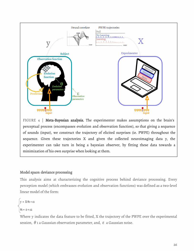
FIGURE 4 | Meta-Bayesian analysis. The experimenter makes assumptions on the brain’s
perceptual process (encompasses evolution and observation function), so that giving a sequence
of sounds (input), we construct the trajectory of elicited surprises (ie. PWPE) throughout the
sequence. Given these trajectories X and given the collected neuroimaging data y, the
experimenter can take turn in being a bayesian observer, by fitting these data towards a
minimization of his own surprise when looking at them.
Model space: deviance processing
This analysis aims at characterizing the cognitive process behind deviance processing. Every
perception model (which embrasses evolution and observation functions) was defined as a two-level
linear model of the form:
Where y indicates the data feature to be fitted, X the trajectory of the PWPE over the experimental
session, θ1 a Gaussian observation parameter, and, ε a Gaussian noise.
26

Following Ostwald et al. , we considered different models to describe the deviance effect, which are
are classified into three families. The famnull family comprises only the null model (Mo), which states
that the brain processes all inputs identically, yielding a trajectory with PWPE always equal to 1.
The famnoL family comprises the ‘change detection’ (CD) and ‘linear change detection’ (LinCD)
models. They are are non-learning models which consider the brain as simply comparing
subsequent sounds. In the CD model, Xk = 0 if there is no change in the sound, X k = 1 in case of a
change. In the LinCD model, X k in case of a change takes a value that depends on the number of
preceding identical sounds. Finally, the famL family comprises Bayesian learning models, which
suppose that the brain makes an estimate of the probability of a standard sound, assuming a
Bernoulli distribution. Indeed, our paradigm recreates in some ways, a biased coin (e.g standard is
head and deviant is tail) with 80% chance to get a head and 20% chance to get a tail. Put simply, one
could picture the brain throwing this coin and tracking, at each toss, the likelihood that heads or
tails will come up. In this example, the internal model of the brain follows a Bernoulli process of
hidden parameter, the probability to get a tail (i.e. deviant). To account for the fact that the brain
may forget about past event, a temporal integration window τ is introduced, whereby distant events
are weighted down. We have been using 5 values of τ: 5, 10, 15, 20 and 25, which makes up 5
models in famL . Each trial’s PWPE measures the belief update about µ using the PWPE (defined as
the Kulback-Leibler divergence between the prior and the posterior distribution of µ).
Within this framework, neural activity reflects the dynamics of Bayesian learning, that is of the
inference on the hidden parameter. To tackle the underlying mechanisms of this bayesian inference
performed by the brain, we consider trial-by-trial changes and we compare them to the
computational variables of the hypothesized internal model.
The whole model space thus included 8 models.
Model space: predictability modulation
The deviance processing analysis revealed bayesian learning models outperforming others. Hence,
this analysis aims at characterizing how predictability modulates the learning that was showed in the
previous analysis.
We refined the perceptual model, by testing the hypothesis that the global structure of the sequence
of sounds influences the dynamic of the perceptual model. Practically speaking, the incrementing
27

structure of the predictable sequences implies that the observer needs to consider at least three
deviants to capture the incrementing session. Hence, it could be that the global temporal structure of
the sequence of sounds induces changes in the depth of the memory involved in the update and in
the prediction.
In this subsequent analysis restricted to the learning model family, we fit the predictable and the
unpredictable conditions separately and investigate a potential difference in the temporal
integration window τ. Precisely, we expected this temporal integration window to be larger when
inverting PF data compared to UF data.
b) Model inversion
Model inversions were performed with the VBA toolbox at each time sample of ECoG time series. To
reduce the number of inversions, we restricted the time interval to - 100 ms to 400 ms sampled at 240
Hz and considered one over 4 samples, leading to 41 samples (hence 41 inversions).
For the deviance analysis, given the 8 models and 9 electrodes, 2952 meta-Bayesian inversions were
carried out for Su78. Individual UF and PF data (4 sessions) were fitted all at once (multi-session
inversions).
For the predictability analysis, given the 1 model, 9 electrodes and the four sessions (PF, UF and
reversed separately), 1476 meta-Bayesian inversions were carried out for Su78. Hence, we have for
each sensor, each sample and each session, an estimated value of τ.
c) Statistical analysis
Analysis 1: Deviance processing
We performed a family model comparison 86 using a fixed-effect analysis (FFX). Our decision
criterion was the family posterior probability, which represents how likely it is that, given our model
space, a family ( famnull, famnoL, famL ) is able to explain the data. We consider that a value of the the
posterior probability greater than 0.75 reflects strong evidence in favor of family fam-noL/L. We
expected Bayesian learning models famL to outperform the famnull and famnoL at the latency of
mismatch responses. For each time-window and location where a family was found significantly
outperforming others, we then compared the relative free energy to precise the winning model
within the winning family.
28

Analysis 2: Predictability effect
We compared the estimated value of τ between conditions (PF and UF).
For each electrode, the statistical analysis was performed over the time samples resulting from the
intersection between the time-windows where the computational modelling for deviance processing
was significant and the time-windows identified by the previous ERP sensor-level analysis
(Kruskal-Wallis statistical test for deviance or predictability).
We then computed the mean and the standard deviation of the estimated τ over the samples of
these selected time-windows and over the two PF (resp. UF) sessions.
Results
We report here findings obtained with Su78, for the ERP analysis (first part) including the typical
analysis of averaged responses and the trial-by-trial modeling approach, and for the spectral analysis
(second part), restricted to the typical analysis of averaged responses.
Post-experimental debriefing with Su78 led us assume that he did not notice the different sound
attributes nor pay attention to the sequence structure. Hence, likewise the original study
(Lecaignard et al 2015), we will assume that any cortical activity difference measured between UF and
PF conditions reflects the implicit learning of the sound sequence regularities.
Preprocessing of data in Su78 led to reject 34 sensors over 92 (see FIG. 5 ), and 24% of events.
Precisely, the number of retained standard trials (standards preceding a deviant sound) was 173 for
the unpredictable sequence and 161 for the predictable sequence. Similarly for deviants, the number
of retained trials was 173 for unpredictable sequence and 169 for the predictable sequence.
FIGURE 5 | Selected sensors resulting from the preprocessing
Small yellow dots depict the position of the 92 sensors on the brain and
large black dots depict the selected ones for further analysis:
- Upper: using CAR referenced data
- Lower: using Bipolar referenced data (then, a rejection of a sensor
leads to the rejection of its neighbor ).
29

A. ERP analysis
The present ERP analysis was conducted with re-referenced data using a bipolar montage (FIG. 3), in
the 2-20 Hz bandwidth.
Results for this section are organized as follows: 1) Responsive sensors identification and clustering;
2) ERP sensor-level ; 3) Computational modelling;
The exact latencies of the significative time-windows that depict figures from part 2), 3), 4) are
detailed in the Supplementary Materials.
a) Responsive sensors
Responsive sensors retained in the present analysis were selected if a significant mismatch effect ( (1)
deviance test, p < 0.001) could be find in either PF or UF condition. As depicted in FIG. 6, we could
identify nine electrodes. As this stage, we clustered these electrodes into two regions of interest with
regard to their anatomical location: the Temporal Gyrus (TG) and Frontal Gyrus (FG).
This tempo-frontal network is aligned with previous findings 5,18,19 and allows us to study the mismatch responses at different stages of the hierarchy.
30

FIGURE 6 | Responsive channels for ERP analysis
Location of the 9 electrodes that showed a statistically
different time-locked response to deviant compared to
standard, grouped with regard to the anatomy.
b) ERP sensor-level
i) Deviance effect
FIG. 7 shows ERPs for the standard and the deviant, as well as the difference between these two
responses in condition UF (red) and PF (green) at the nine responsive electrodes.
In both conditions, standard traces at electrode e37 in primary auditory cortex exhibited a typical
auditory P50-N1-P2 complex.
In condition UF, two significant time-windows for the deviance effect were found: - at the MMN latency: this effect consisted as a succession of significant peaks
starting at electrode e35 (peaking around 130 ms), and followed at e36 and e18
peaking around 180 ms.
- at the P3 latency: this effect starts at e19 and e7 around 260 ms and is followed by a
significant deflection around 330 ms at e18 (which fails to reach significance at
e36).
In addition, it should be noted that an early mismatch effect was found significant at electrode e12, from 55 to 70 ms. In condition PF, a similar temporal (but not spatial) pattern could be observed. Namely:
- at the MMN latency from temporal to frontal electrodes: the effect was found
peaking first around 115 ms at e37, then around 130 ms at e35, and finally
followed by a peak at e30 and e23 around 160 ms.
31

- at the P3 latency over the frontal electrodes: the effect starts at e30 at 214 ms,
followed by a peak at e23 at 250 ms followed by a peak at e12 at 300 ms.
FIGURE 7 | Deviance effect on ERP. Average ERP in bandwidth 2–20 Hz for Su78 elicited by
standards just preceding a deviant (solid line), deviants (dotted line) and the difference responses
(bold solid line) at the shown locations.
The unpredictable condition(UF) is depicted in red (upper row) and the predictable condition(PF)
in green (lower row) . Shaded area correspond to significant time intervals for the comparison of
the deviant and the standard traces (p<0.001).
32

ii) Predictability effect
The effect of predictability was assessed by comparing mismatch, deviant and standard responses
between conditions. FIG.8 displays the difference response for both PF (green) and UF (red)
conditions and the statistically significant time-windows for the predictability effect (p < 0.05).
Predictability effect on the mismatch response: As depicted in blue in FIG. 8, the mismatch response
is significantly modulated with predictability (decrease observed when moving from UF to PF) : - At the latency of the MMN at temporal electrodes e36 and e18.
- At the P3 latency at frontal electrode e7.
Predictability effect on the deviants: When looking at the averaged traces depicted in FIG.8, the
significant effect of predictability on mismatch (e36, e18, e7) could be due to deviant but did not reach
significance. The only effects that reached the significance were:
- at the P3 latency in e19 and e7.
Surprisingly, the main effect on e18 did not come out from this statistical test.
Predictability effect on the standards: As depicted in orange in FIG.8, the response to standards is
significantly modulated with predictability (increase observed when moving from UF to PF) : - At the latency of the MMN at electrodes e18
- At the P3 latency at electrode e18.
33

FIGURE 8 | Predictability effect on ERP. Mismatch responses elicited in PF (green) and the UF
(red) conditions. Grey shadows correspond to the significant time-windows for the deviance
effect (vs.deviant , p < 0.001). Above each graph, the statistically significant time-windows for the
predictability effect (UF vs. PF, p < 0.05) are depicted in blue (predictability effect on the mismatch
signal), orange (predictability effect on the standard response) and purple (predictability effect on
the deviant response).
To sum up these sensor -level analysis:
- We found mismatch at frontal and temporal electrodes, at the MMN and P3
latencies, that validate the significance of our data.
- Only a weak effect of predictability could be measured, at 2 relevant electrodes (at
the MMN-latency in FG and at the P3 latency in FG).
34

- We also measured a strong effect on e18, that would worth further investigations,
insofar as the electrode could eventually capture other non-related activities (e.g
eye movements).
c) Computational modelling
i) Deviance processing
First of all, it should be noted that neither the non-learning nor the learning model significantly
performs during the baseline period. On the post-stimulus period though, results show that learning
models outperforms the null model on the one hand, but more interestingly outperforms the
generally accepted non-learning models on six cortical locations. Hence, PWPE encoding is shown
to participate in the modulation of the low frequency components.
Three time intervals indicated non-null models family outperforming M0: at early latency; at the
latency of the MMN and at the latency of the P3. The components that we had previously identified at
the latency of the MMN were best modelled by family famL (except for two electrodes: e35 and e18 ).
None of our models succeed in model the effect at the MMN latency at e18, and the effect at the P3
latency at electrodes e36, e23, e18, and e12.
FIG 9-a dissect the computational analysis investigation steps:
1) Mismatch traces are plotted for PF (green) and UF (red) conditions.
2) Black shadows from above recall the time-windows that showed a deviance effect in
either of the two conditions.
3) Relative free energy maps obtained at each location for the 7 models (rows) and the 121
samples (columns) between -100 ms and 400 ms around the onset.
4) FFX posterior probability to draw out which family ( famnull, famnoL or famL) best
explains the single-trials variability of the data.
5) Colored shadows corresponds to the time-windows where the FFX probability of famnoL
( orange) or famL (purple) exceeds 0.75. Dark blue time-windows indicates either a
preference for famnull, or for none of the three families.
Figure 9-b show the results of the computational analysis, ie,:
35

1) Identification of a family model if its posterior probability exceeds 0.75.
2) Cross-checking of the models within the winning family and select a winner model
(Bayes factor criterion)
3) Interpretation of the decision with regard to the emerging timeèwindows for
sensors-level statistical tests (grey shadows under the time axis).
One distinguishes the same windows of interest previously identified with the typical Kruskal Wallis
test on deviance. Namely, we found a family that outperformed M0:
- At the MMN latency:
- At e36, e37, e23 and e30, famL (LT with τ of about 10) prevails;
- At e35, the previously identified component (starting at 125 ms) is best
explained by famnoL (CD), but a later one (at 175 ms) seems to be explained
by famL . - At the P3 latency:
- At e35 and e30, greater evidence was found in favour of famnoL (CD)
- At e36 and e19, in favour of famL (LT with τ of about 10)
- At e12 and e18 our model space failed in explaining the variability of the
previously identified component.
- At e7, famnoL (LinCD) hardly pass the significance threshold (one sample).
Also, we could identify new components showing a famnoL/famL-like-dynamic, that did not come out
with a traditional comparison between deviants and standards (Kruskal Wallis deviance test) : - An early latency, at 2 electrodes (e19, e36);
- At the MMN latency, at 3 electrodes (e7, e12, e19);
- At the P3 latency, at 2 electrodes (e30, e35).
36

FIGURE 9a | Investigation steps for the ERP computational analysis (legend for FIG 9-b)
FIGURE 9-b| Results for the ERP computational analysis
37

ii) Predictability modulation
We found 5 electrodes with a non-empty time window intersection between the ERP statistical
analysis and the single-trial statistical analysis.
Though, our estimation of the evolution parameter were not convincing at any identified time
window at e30 and at the early time-window at e36, due to an extremely high variability within the
two sessions of the same condition (PF, UF).
In the above table (FIG. 10), we show the temporal integration window estimated for PF and UF
conditions separately. Considering a bayesian learning of PF (resp. UF) sequence of sounds, the
estimated τ represent the optimal size of the integration window to use in order to model the
dynamic of these selected samples over the trials.
At e7, e35 and e36 (but not at e12), the component identified (around the MMN-latency) led to larger
estimated τ with condition PF compared to condition UF.
For example, if we average the estimation on e35 and e36, we estimate τ at 7.9 for PF and 6.2 for UF.
Considering the fact that sequences were built with a fixed SOA of 600 ms, this translates into
around 3.6 s for PF inversions and 3.7 s for UF inversions. In view of the high variability and slight
difference in the estimates values, these results are not yes fully convincing.
FIGURE 10 | Overview table of results from the single trial computational modelling (analysis 2).
e7 e12 e35 e36
Time-window (ms) 200:225 125:150 100:150 162:200
Number of samples used for the estimation (for each block) 2 2 4 3
Estimated τ for PF (s-1) 6.0±2.1 3.4±0.7 8.2±2.1 7.6±1.7
Estimated τ for UF (s-1) 3.6±0.9 6.6±1.5 6.2±0.6 6.2±1.4
Results of all estimations (inversion computed for each electrode and pooled across reversed sessions
and samples of each identified time-windows) are detailed in the Supplementary Materials.
38

B. Spectral analysis
The present spectral analysis was conducted with re-referenced data using a CAR montage.
This section is organized as follows: 1) alpha envelope in the 8-12 Hz bandwidth; 2) broadband
gamma envelope in the 70-170 Hz bandwidth. For each of these frequency bands, we identified the
responsive sensors and studied both the deviance and the predictability effect.
Responsive sensors retained in the present analysis were selected if they showed a deviance effect for
UF condition (deviant vs. standard, p > 0.001) or a predictability effect regarding standard or deviant
response (PF vs. UF, p < 0.05). The significative time-windows for deviance and predictability effects
on alpha and broadband gamma responses are detailed in the Supplementary Materials.
a) Responsive sensors
Responsive sensors retained in the present analysis were selected if they showed a deviance effect for
UF condition (deviant vs. standard, p > 0.001) or a predictability effect regarding standard or deviant
response (PF vs. UF, p < 0.05).
As depicted in FIG.11, we could identify sixteen electrodes (including one on the left lobe) that we
clustered into frontal (FG) and temporal (TG) gyrus with regard to their anatomical locations.
FIGURE 11 | Responsive channels for spectral
analysis
Location of the 18 electrodes that showed either
a deviance effect (p<0.001) or a predictability
effect (p<0.05) : - For alpha analysis: 18 electrodes
- For broadband gamma: e36 and e37
(primary auditory cortex).
FG states for frontal gyrus and TG for temporal
gyrus.
39

Again, coregistration issues prevent from a reliable interpretation of findings relative to these
anatomical labels. This tempo-frontal network is in line with ERP findings and even show a frontal
activation.
b) Alpha
i) Deviance effect
In condition UF, we identified two temporal electrodes showing a significant effect for deviance (p <
0.001) : e36 and e12. In line with previous findings 87,88 , the response to a deviant sound was
characterized by a lower alpha power for the deviant compared to the standard (around 200-250 ms
after the stimulus onset).
FIGURE 12 | Alpha response to an auditory oddball paradigm. Average alpha envelope (8-12Hz) for
one subject elicited by standards just preceding a deviant (solid line) and deviants (dotted line) at
the shown locations. Only the unpredictable condition is depicted here. Shadowed area correspond
to significant time interval for the comparison of the deviant and the standard traces (p<0.001).
40

ii) Predictability effect
To characterize the influence of the global context on alpha oscillations, we compare the alpha
response to standards and to deviants from UF and PF conditions.
Predictability influence on standards
We found 10 electrodes where alpha responses to standard sounds were modulated by the
predictability context. Precisely:
- At temporal electrodes e36, e37, e11, e18, alpha responses to standard decrease when
moving from UF to PF.
- At frontal electrodes e6 and e47 alpha responses to standard seem to show an
anticipation effect, for the PF condition exclusively, characterized by a decrease of
the alpha response before the onset.
- At frontal electrodes e1, e44, e48 and e5, the modulation goes the other way around
and we found an increase in the alpha response when moving from UF to PF.
41

FIGURE 12| Modulation of alpha responses to standards by predictability. Average alpha
envelope (8-12Hz) for one subject elicited by standards just preceding a deviant in PF (green) and
UF (red) condition at the shown locations. Shadowed area correspond to significant time intervals
for the comparison of the two traces (p < 0.05 ).
Predictability influence on deviants
We found e12 electrodes where alpha responses to deviant sound were modulated by the predictability
context. Precisely:
- In e37 and e38, alpha responses to deviant decrease when moving from UF to PF.
(same trend than for the responses to standard).
42

- In the right TG, electrodes e11 and e18 show the same modulation in the
post-stimulus time-window, that is a decrease of alpha with predictability. In the
left TG (e81), this effect seems to appear earlier.
- Electrodes e12 (TG) and e51 (FG) seem to behave in the opposite way, showing an
increase of alpha level with predictability.
However, we can see along the Sylvian fissure, the propagation of a trough of alpha response to
deviant enhanced in the predictable context. Indeed, we measure a significant trough starting at
around -34.2 ms at e60 (FG), that moves down in the hierarchy to its tempo-lateral neighbors, at
around +13.4 ms at e21 followed by e13 at around + 20.8 ms.
This effect, specific to deviant, suggests that the predictable deviant was in some way, expected.
However, one must be cautious concerning these interpretations, to the extent that we assume, by
omitting on purpose a baseline correction of the trials, that there is not any counterpart at play in the
modulation of alpha power that is not related to the task. For example at e37, it is not sure whether
the effect is due to anticipation or to a pervasive downshift of alpha amplitude from the whole
sequence, specific to the predictable context, or to other undesirable factors.
To sum up, it seems like a predictable auditory input triggers the construction of a tempo-frontal
network, by “switching on” the cortical sites of interest (decreased alpha in some fronto-temporal
electrodes) and “turning off” the others (e.g., increased alpha in e1, e51, e44 and e48). The
interpretation remains unclear with regards to the FG. Hence, the effect at e46 and e40 seeme to come
out later, while e51 and e48 stay up (i.e., low excitability).
43

FIGURE 13 | Modulation of alpha responses to deviants by predictability. Average alpha envelope
(8-12Hz) for one subject elicited by deviants in the predictable (green) and unpredictable (red)
context at the shown locations. Shadowed area correspond to significant time interval for the
comparison of the two traces (p<0.05).
c) Broadband gamma
i) Responsive sensors
We could identify two temporal electrodes (e36 and e37) that showed a significant deviance and
predictability effect in the broadband gamma range.
44

ii) Deviance effect
First, we observe that the amplitude of the broadband gamma response is larger for e36 than for e37,
showing that the excitation of the population underneath the first electrode is greater.
The deviance effect is then characterized in the UF condition by a clear increase in broadband
gamma envelope between 80 and 300 ms after the deviant onset.
Although we did not draw the traces here, we could also identify a deviance effect emerging in the PF
at e35 and e23.
FIGURE 14 | Broadband gamma response to an auditory oddball paradigm. Average broadband
gamma envelope (70-170 Hz) for one subject elicited by standards just preceding a deviant (solid
line) and deviants (dotted line) at the shown locations. Shadowed area correspond to significant
time interval for the comparison of the deviant and the standard traces (p<0.001).
45

iii) Predictability effect
With the same analysis procedure than for ERP and alpha analysis, we found a weak effect of
modulation of the broadband gamma signal with predictability, that would promote a decrease of
broadband gamma mismatch activity with the predictability.
FIGURE 15 | Modulation of broadband gamma responses to deviants by predictability. Average
broadband gamma envelope (70-170Hz) for one subject elicited by deviants in PF (green) and UF
(red) conditions at the shown locations. Shadowed areas correspond to significant time interval for
the comparison of the predictable deviant and the unpredictable deviant (p<0.05).
46

Discussion We studied the ECoG responses of exposed human cortex to auditory oddball sequences during
passive listening. Mismatch activity was characterized by specific ERPs and the modulation of the
spectral components in both the (8-12Hz) and broadband gamma (70-170Hz) range.
A) ERP analysis
a) ERPs measured with ECoG
Our ERP analysis showed that the processing of an oddball sequence involves different levels of the
cortical hierarchy. Precisely, we pointed out a network composed of temporal and frontal lobes in
line with previous findings 5,18,19 . In this network, we identified three post-stimulus time-windows at which the response to deviant
sounds differs from the one to standard sounds: an early effect (before 100 ms), an effect at the MMN
latency (between 100 and 200 ms) and a late one (between 200 and 350 ms).
b) Comment on the choice of a bipolar reference for the ERPs analysis
To analyze ERPs, we chose a bipolar montage instead of a common average reference (CAR). Indeed,
while a common average montage allowed us to reveal the automatic auditory responses, it failed to
discriminate different components of the ERPs although these were later shown to be shaped by the
temporal structure of the sequence. Dürschmid and colleagues (2016), using a slightly different
protocol did not report a predictability effect on the ERPs. The predictability effect was indeed not
emerging using a CAR, which emphasizes the crucial role of the reference montage for the analysis of
low-frequency components84.
c) Predictability effect on the mismatch response
The mismatch response is defined as the difference between the deviant and standard responses. We
found that this difference is shaped by the global structure of the sound sequence. Precisely, the
mismatch response reduces when moving from an unpredictable sequence to a predictable sequence.
This result corroborates, in a single subject, the group-level findings of the original EEG-MEG
study 19.
47

d) Computational analysis
Our computational approach applies to single trial data, with the aim of explaining trial-to-trial
variations of the EcoG signal by the predictable variations of the precision-weighted- prediction error
(PWPE), given a model of the underlying learning process. From the simplest model (null model
assuming no trial to trial variations except noise) to non-learning models (e.g. assuming a simple,
context-independent difference between responses to deviants and standards) and up to Bayesian
learning models (assuming an influence of the history of more or less recently perceived sounds),
these models were fitted to the peri-stimulus data of each sensor where an averaged mismatch
response had been identified.
We revealed three time-windows of interest, in which trial-to-trial changes of the time signals sample
were best explained by one of the learning model. Interestingly, this computational approach allowed
us to highlight some components that did not emerge with the traditional deviance detection
approach on evoked responses. The traditional MMN approach which is equivalent to fitting a
non-learning model, assuming a simple and context-independent difference between responses to
standards and deviants. Furthermore, for the face validity of the approach, it is also important to note
that the null model proved best in the pre-stimulus period. Finally, the fact that a learning model
proved best in some post-stimulus time window demonstrates that mismatch responses are sensitive
to context and reflect learning.
However, some late components eluded our model space. Future work will require an extension of the
model space. For instance, we could consider models that explicitly track the number of standards
before a deviant 18,63.
We could not yet assess the effect of predictability on the temporal integration window used as a
parameter in the Bayesian learning models to explain the variability between PF and UF sequences.
B) Spectral analysis a) Broadband gamma
Our results showed a mismatch response on two electrodes located near the Sylvian fissure,
characterized by a larger amplitude of broadband gamma envelope for deviants compared to
standards.
48

The predictability effect on deviants was found significant on late and very short time-windows,
suggesting a decrease of broadband gamma power with predictability. However, the current analysis
is preliminary and does not allow us to conclude about the precise post-stimulus dynamics of the
high frequency response. Indeed, this activity is highly variable over trials. Further analysis could use
a higher low-pass filter on the envelope of broadband gamma activity or would try to characterize the
distribution of broadband gamma peaks over trials 89.
Traces obtained in temporal cortices were not shaped by predictability, but both predictive coding
hypothesis and Dürschmid’s findings led us to expect that traces from frontal cortices would be
sensitive to the global structure of the sequence71. However, we did not find any frontal electrodes that
showed a significant broadband gamma activity related to the task, contrary to what had been
observed in a similar task.
b) Alpha oscillations
Our findings show a deviance effect in two electrodes from TG, expressed as a larger alpha decrease
(often called “event-related desynchronization”) evoked by a deviant compared to a standard tone.
Let us remind here that previous studies showed that an increase of broadband gamma in response
to deviant led to a later decrease of alpha, interpreted as a bottom-up modulation of alpha ERD.
Hence, the relationship between evoked broadband gamma and alpha ERD in our study could worth
further investigations. We could for example : 1) Evaluate the relative latencies of broadband gamma
peak and alpha trough; 2) Study correlation and Granger-causal interaction between the two
features.
With regards to predictability, care is taken to distinguish two different modulation mechanisms: 1)
In the predictable condition, pervasive alpha level seems to decrease in the involved cortical network
and to increase elsewhere, 2) Some electrodes localized along the Sylvian Fissure showed an
anticipation effect, which was characterized by a short decrease in PF compared to UF prior to the
sound onset (electrode e6 and e60 in FG, and e13 in TG). Interestingly, this expectation marker seems
to be specific to the stimulus category.
However, one must be cautious concerning these interpretations, insofar as:
- The omission of a baseline-correction assumes that there is not any counterpart at
play in the modulation of alpha power that is not related to the task, which is not
guaranteed.
49

- Statistical analysis showed different predictability modulation for responses to
deviants on early latencies (understood as an anticipation) but these did not come
out from the statistical analysis for the deviance effect.
c) Relationship between broadband gamma and alpha
Interestingly, these findings are in line with a more general hypothesis, formulated by Gerwin Schalk 90 as the function-through-biased oscillations (FBO). The FBO postulates that oscillatory alpha voltage
reflects cortical excitability and is responsible for the selection of functional networks involved in a
cognitive task. Put simply, one can imagine the cortex as a relief map and the information as a ‘ball’
constrained on the “cortical landscape”. Alpha would determine the height of the relief and
broadband gamma would express the route taken from the ball tending to go downhill.
The measured modulations of the alpha envelope when averaging across trials can result either from
a decrease in the amplitude of the voltage oscillation in all trials (“background downshifting”) or to a
time-locked desynchronization of neuronal populations driven by thalamic sources (“attention
switch”). The “background downshifting” defines the “cortical landscape” as a whole (ie. low for
engaged populations and high elsewhere). In contrast, the “attention switch” refers to an
event-driven desynchronization leading to a brief decrease in the averaged alpha.
If alpha represents cortical excitability and broadband gamma is a proxy for population level activity,
one would expect that the excitable populations prior to the onset (“attention switch”: alpha decreases
before the onset), would indeed be excited in the post-stimulus time (broadband gamma increases
after the onset). In our data, we measured a decrease in PF compared to UF condition prior to the
stimulus onset in some electrodes, but no significant change in broadband gamma responses
afterwards.
d) Predictive coding and future work
The FBO and the predictive coding hypotheses are compatible and future work should include
interpreting the coupling between alpha and broadband gamma activities in the predictive coding
framework.
50

Precisely, when the FBO hypothesis refers to “cortical excitability” and “population-level activity” as an
interpretation of a decrease in alpha voltage and an increase in broadband gamma power respectively,
the predictive coding hypothesis refers to “precision” and “prediction error”.
Hence, we could keep the same model-space used for the ERP single-trial analysis and defined in the
methods and adapt the observation functions from ERP to spectral features (alpha and broadband
gamma envelopes).
One initial approach consists in : 1) Extracting alpha and broadband gamma power averaged on the
identified significant time-windows and, 2) Fitting separately the precision, the prediction error and
the precision-weighted prediction error (PWPE) to the two spectral features.
C) ECoG limitations
ECoG allows fine spatial localization of effects as well as an exceptionally high signal-to-noise ratio.
On the hand, cortical coverage is limited compared to scalp recordings, that may provide a better
global picture of the phenomenon of interest.
Critically, coregistration issues prevent from a reliable interpretation of findings relative to these
anatomical labels. It remains possible that some electrodes from the FG (e.g e30, e23) capture activity
generated in the superior temporal plane. In the same vein, electrodes in the TG could reflect an
inferior frontal activity (e.g e12).
Furthermore, the number of recordable patients is limited and one has to carefully clean the signals
from pathological waveforms.
D) Number of subjects
These early analysis on a single-subject are showing very promising results that beg to be confirmed
and completed with future subjects.
The fourth involved patient (Su81) was implanted with a high density grid (232 electrodes - 2 mm
diameter, 1.0 mm exposed), which allows even more precise spatial localization. Co-registration
issues are again to be considered carefully when clustering the sensors with regards to the functional
anatomy. Although, in order to perform a group-level analysis, it is crucial to cluster the responsive
sensors.
51

Supplementary material:
A) ECoG clinical and research procedure
52

B) Patient rejection
a) Epilepsy of patient Su79
FIGURE 16 | Raw signals of patient Su79. The epileptical activity is recognized by an abnormal
synchronization of the signals across channels. It is characterized by an activity pattern that is not
physiological but pathological.
53

b) Screening of patient Su80
FIGURE 17 | Brain mapping of patient Su80. We perform a screening in order to identify the
location of the brain networks involved in different cognitive process in order to assure that the
seizure focus can be removed without causing damage to important nearby brain regions. For this
aim, we consider broadband gamma power evoked by the screening task (eg. listen to music, speak,
moving the tongue…). In the above figure, each red dot represents an electrode and its size the level
of broadband gamma evoked by the auditory (here listening to voice, music, foreign language) task.
For patient Su80, there were no responsive electrodes for auditory tasks, so he could not take part to
any experiments.
54

C) Detailed results from statistical analysis
a) ERP analysis
i) Sensor-level analysis
FIGURE 18 | Significant (p<0.001) time-windows resulting from the Kruskal-Wallis statistical tests for
deviance effect (ie. standards vs. deviants for PF and UF separately) and the predictability effect (ie. PF
vs. UF for standards and deviants separately).
Significant post-stimulus time windows (in ms) e7 e12 e18 e19 e23 e30 e35 e36 e37
Deviance effect (UF) p<0.001 267:315 58:66
166:229; 296:364 265:305 X X 106:148 161:202 X
Deviance effect (PF) p<0.001 X 291:307 X X
167:188; 232:267
137:15 ; 222:244 114:47 X 117:122
Predictability effect on standards - p<0.05 82:119 129:148
164:173 ; 352:383 58:68 58:68 X 54:87 X 62:82
Predictability effect on deviants - p<0.05
206:226; 252:287 X X 268:298 59:67 60:77 60:77
65:82; 371:179 X
Predictability effect on difference (p<0.05)
252:272; 337:346 X 153:228 X X X X
82:100; 110:127; 202:223 X
Single-trial computational analysis effect (FFX log-posterior probability> 0.75) 200:225 100:150 X
62:125 ; 175:187 X
125:187; 225:250
100:150; 187:200; 225:287
75:112; 162:225 137:150
55

ii) Computational analysis
FIGURE 19 | Predictability effect on the computational analysis: Posterior mean and standard deviation of 𝜏 estimated on PF and UF blocks separately. Average is performed on : A) Samples with FFX log-posterior probability exceeding 0.75; B) Samples with FFX log-posterior probability exceeding 0.75 and with a significant deviance effect (Kruskall-Wallis p>0.001) ; C) Samples with FFX log-posterior probability exceeding 0.75 and with a significant predictability effect (Kruskall-Wallis p>0.05) Significant post-stimulus time windows (in ms) e7 e12 e18 e19 e23 e30 e35 e36 e37
A) Time windows relevant from the single-trial analysis effect (FFX log-posterior probability> 0.75) 200:225 100:150 X
62:125; 175:187 X
125:187; 225:250
100:150; 187:200; 225:287 75:100 ; 137:150
mean, std of 𝜏 estimated for PF blocks on the above time-windows (A) 6.0±2.1 3.8±0.8 X
10.8±6.2; 4.9±0.8 X
8.1-1.6; 8.2±2.2
8.2±2.1; 15.2±14.3; 14.5±9.6 11.5±8.9; 4.4±0.7
mean, std of 𝜏 estimated for UF blocks on the above time-windows (A) 3.6±0.9 6.6±1.4 X
6.5±0.15; 6.01±5.5 X
17.6±17.6; 9.8±7.7
6.2±0.6; 9.5±7.1; 13.8±13.7 6.5±1.3; 10.8±1.4
B)Intersection of time-windows from “deviance” and “single-trial” analysis X X X X X
125:150; 225:250 100:150 162:200 X
mean, std of 𝜏 estimated for PF blocks on the above time-windows (B) X X X X X
6.8±1.8; 8.2±2.2 8.2±2.1 7.6±1.7 X
mean, std of 𝜏 estimated for UF blocks on the above time-windows (B) X X X X X
24.5±21.6; 9.8±7.7 6.2±0.6 6.2±1.4 X
C)Intersection of time-windows from “predictability” and “single-trial” analysis 200:225 125:150 X X X X X 75:82 X
mean, std of 𝜏 estimated for PF blocks on the above time-windows (C) 6.0±2.1 3.4±0.7 X X X X X 15.9±13.5 X
mean, std of 𝜏 estimated for UF blocks on the above time-windows (C) 3.6±0.9 6.6±1.5 X X X X X 6.8±1.9 X
56

b) Spectral analysis
i) Sensor-level analysis for alpha
FIGURE 20 | Statistics on alpha responses: Significant (p<0.001) time-windows resulting from the
Kruskal-Wallis statistical tests for deviance effect (ie. standards vs. deviants for PF and UF separately)
and the predictability effect (ie. PF vs. UF for standards and deviants separately).
Significant post-stimulus time windows (in ms) e1 e6 e11 e12 e13 e18 e21 e36 e37
Deviance effect (UF) p<0.001 X X X 260:320 X X X 300:330 X
Deviance effect (PF) p<0.001 X -110:-70 X X X X X X X
Predictability on standards (p<0.05) -20:+220 -130:-40 -90:170 X X 260:300 X
10:70; 310:380 30:380
Predictability on deviants (p<0.05) X X 20:130 250:320 -20:-60 130:240 50:140 -200:-150 -200:-110
Significant post-stimulus time windows (in ms) e38 e40 e44 e46 e47 e48 e51 e60 e81
Deviance effect (UF) p<0.001 X X X X X X X X X
Deviance effect (PF) p<0.001 X X X X X X X X X
Predictability on standards (p<0.05) X X 300:380 X -160:-50 -10:160 -20:260 X X
Predictability on deviants (p<0.05) 20:120 190:370 X 230:320 X -200:-120 220:300
-140:-70; 250:280 -40:50
57

ii) Sensor-level analysis for broadband gamma
FIGURE 21 | Statistics on broadband gamma
responses: Deviance and Predictability.
Significant post-stimulus time windows (in ms) e35 e36 e37
Deviance effect (UF) p<0.001 X
89:109; 39:149; 209:259 229:239
Deviance effect (PF) p<0.001
119:169; 229:239 X X
Predictability on standards (p<0.05) X X X
Predictability on deviants (p<0.05) X
80:100; 230:270
10:30; 240:260
58

Bibliography
1. Dehaene, S., Meyniel, F., Wacongne, C., Wang, L. & Pallier, C. The Neural Representation of
Sequences: From Transition Probabilities to Algebraic Patterns and Linguistic Trees. Neuron
88, 2–19 (2015).
2. Conway, C. M., Karpicke, J. & Pisoni, D. B. Contribution of implicit sequence learning to
spoken language processing: Some preliminary findings with hearing adults. J. Deaf Stud.
Deaf Educ. 12, 317–334 (2007).
3. Romberg, A. R. & Saffran, J. R. Statistical learning and language acquisition. Wiley Interdiscip.
Rev. Cogn. Sci. 1, 906–914 (2010).
4. Rohrmeier, M. & Rebuschat, P. Implicit Learning and Acquisition of Music. Top. Cogn. Sci. 4,
525–553 (2012).
5. Ostwald, D. et al. Evidence for neural encoding of Bayesian surprise in human
somatosensation. Neuroimage 62, 177–188 (2012).
6. Pazo-Alvarez, P., Cadaveira, F. & Amenedo, E. MMN in the visual modality: a review. Biol.
Psychol. 63, 199–236 (2003).
7. Garrido, M. I., Kilner, J. M., Stephan, K. E. & Friston, K. J. The mismatch negativity: a review
of underlying mechanisms. Clin. Neurophysiol. 120, 453–463 (2009).
8. Horváth, J., Müller, D., Weise, A. & Schröger, E. Omission mismatch negativity builds up late.
Neuroreport 21, 537–541 (2010).
9. Näätänen, R., Gaillard, A. W. & Mäntysalo, S. Early selective-attention effect on evoked
59

potential reinterpreted. Acta Psychol. 42, 313–329 (1978).
10. Näätänen, R. The role of attention in auditory information processing as revealed by
event-related potentials and other brain measures of cognitive function. Behav. Brain Sci. 13,
201–233 (1990).
11. Näätänen, R. Attention and Brain Function. (Lawrence Erlbaum Associates, 1992).
12. Näätänen, R., Tervaniemi, M., Sussman, E., Paavilainen, P. & Winkler, I. ‘Primitive
intelligence’ in the auditory cortex. Trends Neurosci. 24, 283–288 (2001).
13. Basirat, A., Dehaene, S. & Dehaene-Lambertz, G. A hierarchy of cortical responses to
sequence violations in three-month-old infants. Cognition 132, 137–150 (2014).
14. Morlet, D. & Fischer, C. MMN and novelty P3 in coma and other altered states of
consciousness: a review. Brain Topogr. 27, 467–479 (2014).
15. Ruby, P., Caclin, A., Boulet, S., Delpuech, C. & Morlet, D. Odd sound processing in the
sleeping brain. J. Cogn. Neurosci. 20, 296–311 (2008).
16. Chennu, S. & Bekinschtein, T. A. Arousal modulates auditory attention and awareness:
insights from sleep, sedation, and disorders of consciousness. Front. Psychol. 3, 65 (2012).
17. Näätänen, R., Paavilainen, P., Rinne, T. & Alho, K. The mismatch negativity (MMN) in basic
research of central auditory processing: a review. Clin. Neurophysiol. 118, 2544–2590 (2007).
18. Lieder, F., Daunizeau, J., Garrido, M. I., Friston, K. J. & Stephan, K. E. Modelling trial-by-trial
changes in the mismatch negativity. PLoS Comput. Biol. 9, e1002911 (2013).
19. Lecaignard, F., Bertrand, O. & Gimenez, G. Implicit learning of predictable sound sequences
modulates human brain responses at different levels of the auditory hierarchy. Front. Hum.
Neurosci. (2015).
20. David, O. et al. Dynamic causal modeling of evoked responses in EEG and MEG. Neuroimage
30, 1255–1272 (2006).
60
21. Haegens, S., Nácher, V., Luna, R., Romo, R. & Jensen, O. α-Oscillations in the monkey
sensorimotor network influence discrimination performance by rhythmical inhibition of
neuronal spiking. Proc. Natl. Acad. Sci. U. S. A. 108, 19377–19382 (2011).
22. Barry, R. J., Clarke, A. R., Johnstone, S. J., Magee, C. A. & Rushby, J. A. EEG differences
between eyes-closed and eyes-open resting conditions. Clin. Neurophysiol. 118, 2765–2773
(2007).
23. Crone, N. E., Boatman, D., Gordon, B. & Hao, L. Induced electrocorticographic gamma
activity during auditory perception. Clin. Neurophysiol. 112, 565–582 (2001/4).
24. Lehtelä, L., Salmelin, R. & Hari, R. Evidence for reactive magnetic 10-Hz rhythm in the
human auditory cortex. Neurosci. Lett. 222, 111–114 (1997).
25. Pfurtscheller, G. & Aranibar, A. Evaluation of event-related desynchronization (ERD)
preceding and following voluntary self-paced movement. Electroencephalogr. Clin. Neurophysiol.
46, 138–146 (1979).
26. Neuper, C., Wörtz, M. & Pfurtscheller, G. ERD/ERS patterns reflecting sensorimotor
activation and deactivation. Prog. Brain Res. 159, 211–222 (2006).
27. Deiber, M.-P. et al. EEG alpha activity reflects motor preparation rather than the mode of
action selection. Front. Integr. Neurosci. 6, 59 (2012).
28. Tamura, Y. et al. Functional relationship between human rolandic oscillations and motor
cortical excitability: an MEG study. Eur. J. Neurosci. 21, 2555–2562 (2005).
29. Romei, V., Rihs, T., Brodbeck, V. & Thut, G. Resting electroencephalogram alpha-power over
posterior sites indexes baseline visual cortex excitability. Neuroreport 19, 203–208 (2008).
30. Sauseng, P., Klimesch, W., Gerloff, C. & Hummel, F. C. Spontaneous locally restricted EEG
alpha activity determines cortical excitability in the motor cortex. Neuropsychologia 47,
284–288 (2009).
61

31. Ergenoglu, T. et al. Alpha rhythm of the EEG modulates visual detection performance in
humans. Brain Res. Cogn. Brain Res. 20, 376–383 (2004).
32. Linkenkaer-Hansen, K., Nikulin, V. V., Palva, S., Ilmoniemi, R. J. & Palva, J. M. Prestimulus
oscillations enhance psychophysical performance in humans. J. Neurosci. 24, 10186–10190
(2004).
33. Thut, G., Nietzel, A., Brandt, S. A. & Pascual-Leone, A. Alpha-band electroencephalographic
activity over occipital cortex indexes visuospatial attention bias and predicts visual target
detection. J. Neurosci. 26, 9494–9502 (2006).
34. Hanslmayr, S. et al. Prestimulus oscillations predict visual perception performance between
and within subjects. Neuroimage 37, 1465–1473 (2007).
35. Romei, V., Gross, J. & Thut, G. On the role of prestimulus alpha rhythms over occipito-parietal
areas in visual input regulation: correlation or causation? J. Neurosci. 30, 8692–8697 (2010).
36. Lange, J., Oostenveld, R. & Fries, P. Reduced occipital alpha power indexes enhanced
excitability rather than improved visual perception. J. Neurosci. 33, 3212–3220 (2013).
37. Mazaheri, A. et al. Region-specific modulations in oscillatory alpha activity serve to facilitate
processing in the visual and auditory modalities. Neuroimage 87, 356–362 (2014).
38. Bauer, M. et al. Cholinergic enhancement of visual attention and neural oscillations in the
human brain. Curr. Biol. 22, 397–402 (2012).
39. Jensen, O. & Mazaheri, A. Shaping functional architecture by oscillatory alpha activity: gating
by inhibition. Front. Hum. Neurosci. 4, 186 (2010).
40. Klimesch, W., Sauseng, P. & Hanslmayr, S. EEG alpha oscillations: the inhibition-timing
hypothesis. Brain Res. Rev. 53, 63–88 (2007).
41. Weisz, N., Hartmann, T., Müller, N., Lorenz, I. & Obleser, J. Alpha rhythms in audition:
cognitive and clinical perspectives. Front. Psychol. 2, 73 (2011).
62
42. Mazaheri, A. & Jensen, O. Rhythmic pulsing: linking ongoing brain activity with evoked
responses. Front. Hum. Neurosci. 4, 177 (2010).
43. Brandt, M. E. & Jansen, B. H. The relationship between prestimulus-alpha amplitude and
visual evoked potential amplitude. Int. J. Neurosci. 61, 261–268 (1991).
44. Gruber, W. R., Klimesch, W., Sauseng, P. & Doppelmayr, M. Alpha phase synchronization
predicts P1 and N1 latency and amplitude size. Cereb. Cortex 15, 371–377 (2005).
45. Haig, A. R. & Gordon, E. EEG alpha phase at stimulus onset significantly affects the
amplitude of the P3 ERP component. Int. J. Neurosci. 93, 101–115 (1998).
46. Palva, S. & Palva, J. M. New vistas for alpha-frequency band oscillations. Trends Neurosci. 30,
150–158 (2007).
47. Klimesch, W. α-band oscillations, attention, and controlled access to stored information.
Trends Cogn. Sci. 16, 606–617 (2012).
48. Manning, J. R., Jacobs, J., Fried, I. & Kahana, M. J. Broadband shifts in local field potential
power spectra are correlated with single-neuron spiking in humans. J. Neurosci. 29,
13613–13620 (2009).
49. Crone, N. E. et al. Functional mapping of human sensorimotor cortex with
electrocorticographic spectral analysis. I. Alpha and beta event-related desynchronization.
Brain 121 ( Pt 12), 2271–2299 (1998).
50. Miller, K. J. et al. Real-time functional brain mapping using electrocorticography. Neuroimage
37, 504–507 (2007).
51. Kubánek, J., Miller, K. J., Ojemann, J. G., Wolpaw, J. R. & Schalk, G. Decoding flexion of
individual fingers using electrocorticographic signals in humans. J. Neural Eng. 6, 066001
(2009).
52. Canolty, R. T. et al. Spatiotemporal dynamics of word processing in the human brain. Front.
63

Neurosci. 1, 185–196 (2007).
53. Potes, C., Brunner, P., Gunduz, A., Knight, R. T. & Schalk, G. Spatial and temporal
relationships of electrocorticographic alpha and gamma activity during auditory processing.
Neuroimage 97, 188–195 (2014).
54. Sturm, I., Blankertz, B., Potes, C., Schalk, G. & Curio, G. ECoG high gamma activity reveals
distinct cortical representations of lyrics passages, harmonic and timbre-related changes in a
rock song. Front. Hum. Neurosci. 8, 798 (2014).
55. Zion Golumbic, E. M. et al. Mechanisms underlying selective neuronal tracking of attended
speech at a ‘cocktail party’. Neuron 77, 980–991 (2013).
56. Dijkstra, K. et al. Identifying the Attended Speaker Using Electrocorticographic (ECoG)
Signals. Brain Comput Interfaces (Abingdon) 2, 161–173 (2015).
57. Gunduz, A. et al. Neural correlates of visual-spatial attention in electrocorticographic signals
in humans. Front. Hum. Neurosci. 5, 89 (2011).
58. Gunduz, A. et al. Decoding covert spatial attention using electrocorticographic (ECoG) signals
in humans. Neuroimage 60, 2285–2293 (2012).
59. Edwards, E. et al. Comparison of time-frequency responses and the event-related potential to
auditory speech stimuli in human cortex. J. Neurophysiol. 102, 377–386 (2009).
60. Pei, X., Barbour, D. L., Leuthardt, E. C. & Schalk, G. Decoding vowels and consonants in
spoken and imagined words using electrocorticographic signals in humans. J. Neural Eng. 8,
046028 (2011).
61. Cervenka, M. C., Nagle, S. & Boatman-Reich, D. Cortical high-gamma responses in auditory
processing. Am. J. Audiol. 20, 171–180 (2011).
62. Friston, K. & Kiebel, S. Predictive coding under the free-energy principle. Philos. Trans. R. Soc.
Lond. B Biol. Sci. 364, 1211–1221 (2009).
64

63. Lecaignard, F. Predictive coding in auditory processing : insights from advanced modeling of
EEG and MEG mismatch responses. (Université de Lyon, , 2016).
64. Bastos, A. M. et al. Canonical microcircuits for predictive coding. Neuron 76, 695–711 (2012).
65. Bauer, M. Functional roles of rhythmic neuronal activity in the human visual and somatosensory
system. ([Sl: sn], 2008).
66. Fogelson, N., Shah, M., Scabini, D. & Knight, R. T. Prefrontal cortex is critical for contextual
processing: evidence from brain lesions. Brain 132, 3002–3010 (2009).
67. Lara, A. H. & Wallis, J. D. The Role of Prefrontal Cortex in Working Memory: A Mini Review.
Front. Syst. Neurosci. 9, 173 (2015).
68. Deouell, L. Y. The Frontal Generator of the Mismatch Negativity Revisited. J. Psychophysiol. 21,
188–203 (2007).
69. Rosburg, T. et al. Subdural recordings of the mismatch negativity (MMN) in patients with
focal epilepsy. Brain 128, 819–828 (2005).
70. Muthukumaraswamy, S. D. High-frequency brain activity and muscle artifacts in MEG/EEG:
a review and recommendations. Front. Hum. Neurosci. 7, 138 (2013).
71. Dürschmid, S. et al. Hierarchy of prediction errors for auditory events in human temporal
and frontal cortex. Proc. Natl. Acad. Sci. U. S. A. 113, 6755–6760 (2016).
72. Sedley, W. et al. Neural signatures of perceptual inference. eLife Sciences 5, e11476 (2016).
73. Litvak, V. & Friston, K. Electromagnetic source reconstruction for group studies. Neuroimage
42, 1490–1498 (2008).
74. Lecaignard, F., Bertrand, O., Caclin, A. & Mattout, J. Empirical evaluation of fused MEG-EEG
source reconstruction applied to auditory mismatch generators. in preparation 28, 14301–14310
(2017).
75. Edwards, E., Soltani, M., Deouell, L. Y., Berger, M. S. & Knight, R. T. High gamma activity in
65

response to deviant auditory stimuli recorded directly from human cortex. J. Neurophysiol. 94,
4269–4280 (2005).
76. Sinai, A. et al. Intracranial mapping of auditory perception: event-related responses and
electrocortical stimulation. Clin. Neurophysiol. 120, 140–149 (2009).
77. Phillips, H. N. et al. Convergent evidence for hierarchical prediction networks from human
electrocorticography and magnetoencephalography. Cortex 82, 192–205 (2016).
78. Komatsu, M., Takaura, K. & Fujii, N. Mismatch negativity in common marmosets:
Whole-cortical recordings with multi-channel electrocorticograms. Sci. Rep. 5, 15006 (2015).
79. Fishman, Y. I. & Steinschneider, M. Searching for the mismatch negativity in primary
auditory cortex of the awake monkey: deviance detection or stimulus specific adaptation? J.
Neurosci. 32, 15747–15758 (2012).
80. El Karoui, I. et al. Event-Related Potential, Time-frequency, and Functional Connectivity
Facets of Local and Global Auditory Novelty Processing: An Intracranial Study in Humans.
Cereb. Cortex 25, 4203–4212 (2015).
81. Eliades, S. J. et al. Adaptation of high-gamma responses in human auditory association
cortex. J. Neurophysiol. 112, 2147–2163 (2014).
82. Daunizeau, J. et al. Observing the observer (I): meta-bayesian models of learning and
decision-making. PLoS One 5, e15554 (2010).
83. Besle, J. et al. Visual activation and audiovisual interactions in the auditory cortex during
speech perception: intracranial recordings in humans. J. Neurosci. 28, 14301–14310 (2008).
84. Liu, Y., Coon, W. G., de Pesters, A., Brunner, P. & Schalk, G. The effects of spatial filtering and
artifacts on electrocorticographic signals. J. Neural Eng. 12, 056008 (2015).
85. Daunizeau, J., Adam, V. & Rigoux, L. VBA: a probabilistic treatment of nonlinear models for
neurobiological and behavioural data. PLoS Comput. Biol. 10, e1003441 (2014).
66

86. Penny, W. D. et al. Comparing families of dynamic causal models. PLoS Comput. Biol. 6,
e1000709 (2010).
87. Haenschel, C., Baldeweg, T., Croft, R. J., Whittington, M. & Gruzelier, J. Gamma and beta
frequency oscillations in response to novel auditory stimuli: A comparison of human
electroencephalogram (EEG) data with in vitro models. Proc. Natl. Acad. Sci. U. S. A. 97,
7645–7650 (2000).
88. Barry, R. J., Kirkaikul, S. & Hodder, D. EEG alpha activity and the ERP to target stimuli in an
auditory oddball paradigm. Int. J. Psychophysiol. 39, 39–50 (2000).
89. Coon, W. G. & Schalk, G. A method to establish the spatiotemporal evolution of task-related
cortical activity from electrocorticographic signals in single trials. J. Neurosci. Methods 271,
76–85 (2016).
90. Schalk, G. A general framework for dynamic cortical function: the
function-through-biased-oscillations (FBO) hypothesis. Front. Hum. Neurosci. 9, 352 (2015).
67