implicit filtering for image and shape...
TRANSCRIPT
Vision, Image & Signal Processing (VISP)
Implicit Filtering for
Image and Shape Processing
Alex Belyaev Electrical, Electronic & Computer Engineering
School of Engineering & Physical Sciences
Heriot-Watt University
Edinburgh
Implicit filtering and its applications
A. Belyaev, “On implicit image derivatives and their
applications.” BMVC 2011, Dundee, Scotland, UK, August 2011.
A. Belyaev and H. Yamauchi, “Implicit filtering for image and
shape processing.” VMV 2011, Berlin, Germany, October 2011.
A. Belyaev, B. Khesin, and S. Tabachnikov, “Discrete speherical
means of directional derivatives and Veronese maps.” Journal of
geometry and Physics, 2011. Accepted.

Implicit vs explicit
1 1
1 1 1 1
1
2
1 1
2 2
i i i
i i i i i
f f fh
f w f f f fw h
1if
if1if
h h
Discrete
signal
sampled
regularly
with
spacing h
Standard explict finite difference scheme
An implicit finite
difference scheme
2 24
2
24
2
4
2 6
12
6
14 , 1
6
f x h f x h h df x f x O h
h dx
hf x f x h f x f x h O h
h
f x h f x f x h O h h
w=4 gives a higher
approximation order
for small h.

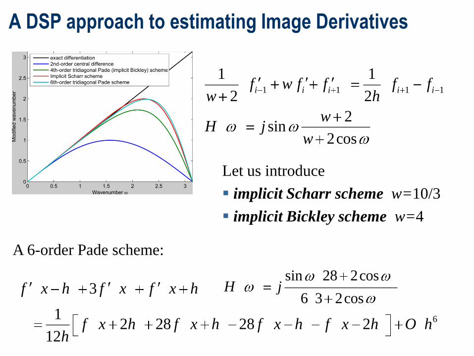
A DSP approach to estimating Image Derivatives
frequency response, 1
1 -
1 1sin
2
j x
j x j x
L e H j
h
d de j e j
dx dx
f x f xj
Delivers a good approximation
of jω for small ω only
Implicit finite differences: an example
434f x h f x f x h f x h f x h O h
h
Non-causal IIR filters in the DSP language
Rational (Pade) approximations in Maths
3sin
2 cosH j
A DSP approach to estimating Image Derivatives
6
3
12 28 28 2
12
f x h f x f x h
f x h f x h f x h f x h O hh
1 1 1 1
1 1
2 2
2sin
2cos
i i i i if w f f f fw h
wH j
w
sin 28 2cos
6 3 2cosH j
A 6-order Pade scheme:
Let us introduce
implicit Scharr scheme w=10/3
implicit Bickley scheme w=4

2 2 2222 2 2 2 2
2 2 2 2, , , 2
x
yx y x y x x y y
Commonly used discrete gradients & Laplacians Rotation-invariant differential quantities (operators) used widely in
Image Processing and Computer Vision:
Need for accurate discrete approximations. The standard discrete
approximations are not sufficiently accurate.
1 0 11
02 2
1 0 1
w wx h w
1 (Prewitt, 1970)
2 (Sobel, 1970)
10 3 (Scharr, 2000)
4 (Bickley, 1947)
simple symmetric f.d.
w
w
w
w
w
1 (Gonzalez &Woods)
2 (Kamgar-Parsi & Resenfeld, 1999)
4 Mehrstellen Laplacian
standard 5-point stencil
w
w
w
w
2
1 11
4 12
1 1
w
w w wh w
w
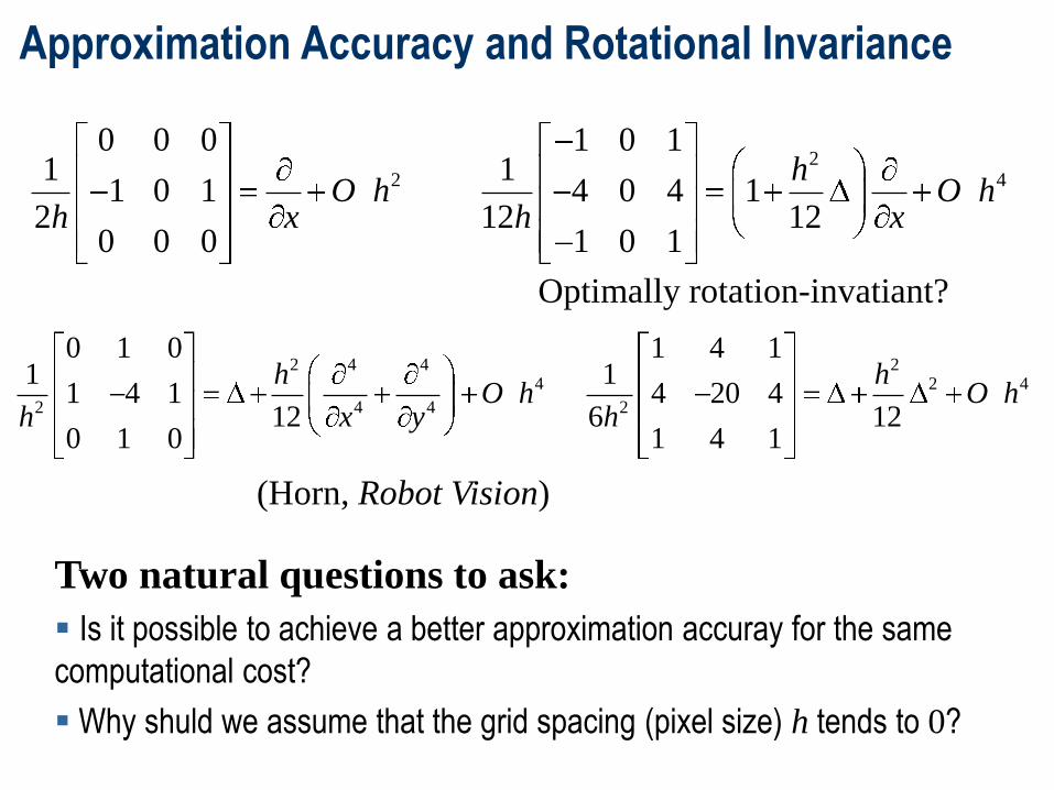
Approximation Accuracy and Rotational Invariance
22 4
0 0 0 1 0 11 1
1 0 1 4 0 4 12 12 12
0 0 0 1 0 1
hO h O h
h x h x
2 4 4 24 2 4
2 4 4 2
0 1 0 1 4 11 1
1 4 1 4 20 412 6 12
0 1 0 1 4 1
h hO h O h
h x y h
(Horn, Robot Vision)
Optimally rotation-invatiant?
Two natural questions to ask:
Is it possible to achieve a better approximation accuray for the same
computational cost?
Why shuld we assume that the grid spacing (pixel size) h tends to 0?
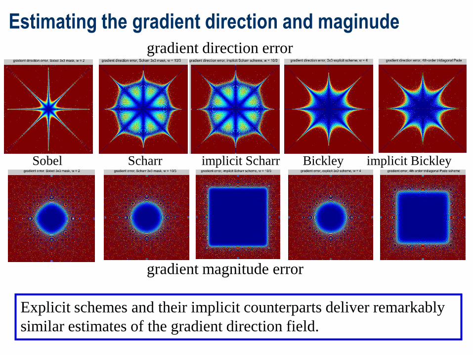
Estimating the gradient direction and maginude gradient direction error
Sobel Scharr implicit Scharr Bickley implicit Bickley
gradient magnitude error
Explicit schemes and their implicit counterparts deliver remarkably
similar estimates of the gradient direction field.

Explicit vs. Implicit
1 0 11
02 2
1 0 1
w wx h w
1 1 1
1 1
1
2
1
2
i i i
i i
f w f fw
f fh
Smoothing introduced by
[-1 0 1]/2 in x-direction is
compensated by applying
[1 w 1]/(w+2) smoothing
in y-direction
Smoothing introduced by
[-1 0 1]/2 in x-direction is
comensated by applying
[1 w 1]/(w+2) smoothing
to the derivative.
Given an explicit scheme and its implicit counterpart, both the schemes
produce similar estimates of the gradient direction, however the
implicit scheme does a better job in estimating the gradient magnitude.

High-resolution schemes
2 1 1 2
1 1 2 2 3 32 4 6
sin 2 sin 2 3 sin 3
1 2 cos 2 cos 2
i i i i i
i i i i i i
f f f f f
a b cf f f f f f
a bH j
S. K. Lele, “Compact finite difference
schemes with spectral like resolution.”
Journal of Computational Physics, 1992.
Lele scheme: 0.5771439, 0.0896406
1.302566, 0.99355, 0.03750245a b c

Fourier-Pade-Galerkin approximations 1
Space or trigonometric
polynomials of degree N
span :jn
N e N n NF
Rational Fourier series
,
kl k l
k k l l
R P Q
P QF F
, ,
0
is a properly chosen weighting function.
kl
l k k l
f R
Q f P g W d g
W
F
It gives a system of k+l lnear equations with k+l unknowns.
In our case, k=3 and l=2. 3
2
sin 2 sin 2 3 sin 3
1 2 cos 2 cos 2
P a b
Q

Fourier-Pade-Galerkin approximations 2 A system of k+l linear equations with k+l unknowns. k=3 and l=2.
1W

Fourier-Pade-Galerkin approximations 3 A system of k+l linear equations with k+l unknowns. k=3 and l=2.
1 0 0.9
0 0.9W

Fourier-Pade-Galerkin approximations 4
Lele scheme
1W
1 0 0.9
0 0.9W
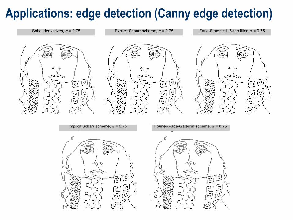
Applications: edge detection (Canny edge detection)
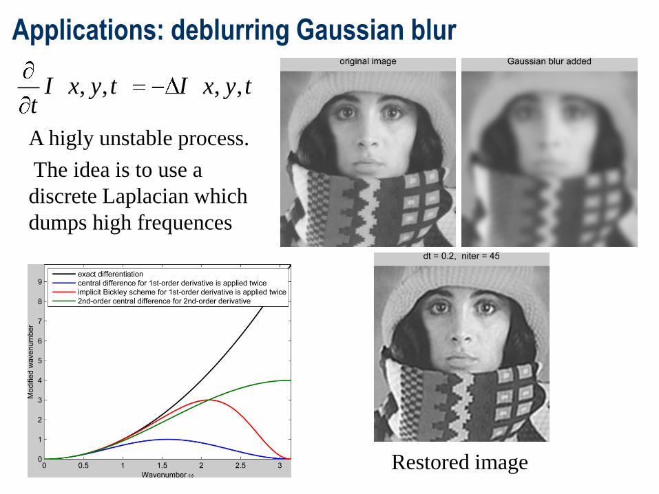
Applications: deblurring Gaussian blur
, , , ,I x y t I x y tt
A higly unstable process.
The idea is to use a
discrete Laplacian which
dumps high frequences
Restored image
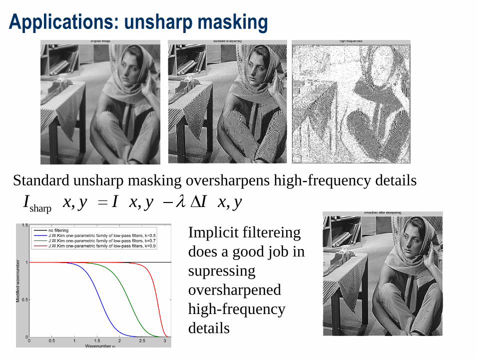
Applications: unsharp masking
sharp , , ,I x y I x y I x y
Standard unsharp masking oversharpens high-frequency details
Implicit filtereing
does a good job in
supressing
oversharpened
high-frequency
details

Implicit
filtering
1 1
1 1
1 ˆ ˆ ˆ1 2
12
4
1 2 1 cos
1 cos 2
1 21,
1 2
i i i
i i i
f f f
f f f
H
p
frequency
response
function
1
2
,
2 2 2
2, 2 2
1 tan , 1,2,3,2
1 2 as 0
1as
2
p
p
p p
pp p
H p
O
HO
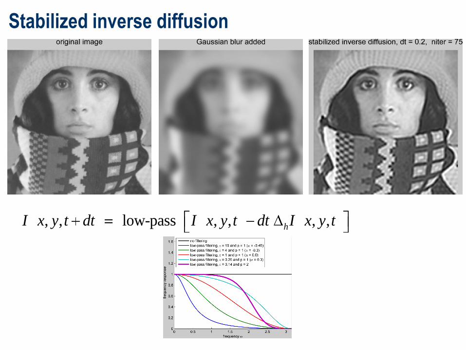
Stabilized inverse diffusion
, , low-pass , , , ,hI x y t dt I x y t dt I x y t

Implicit filtering and approximation subdivision
1 1 1 1
1 1ˆ ˆ ˆ 21 2 4
1 2 1 cos
1 cos 2
i i i i i if f f f f f
H
1 1 1
2 2 1 1
1 1 1 1
1,
2
1 1 1
1 2 2 4
k k k k k
i i i i i
k k k k k k
i i i i i i
u v u v v
v v v u u u
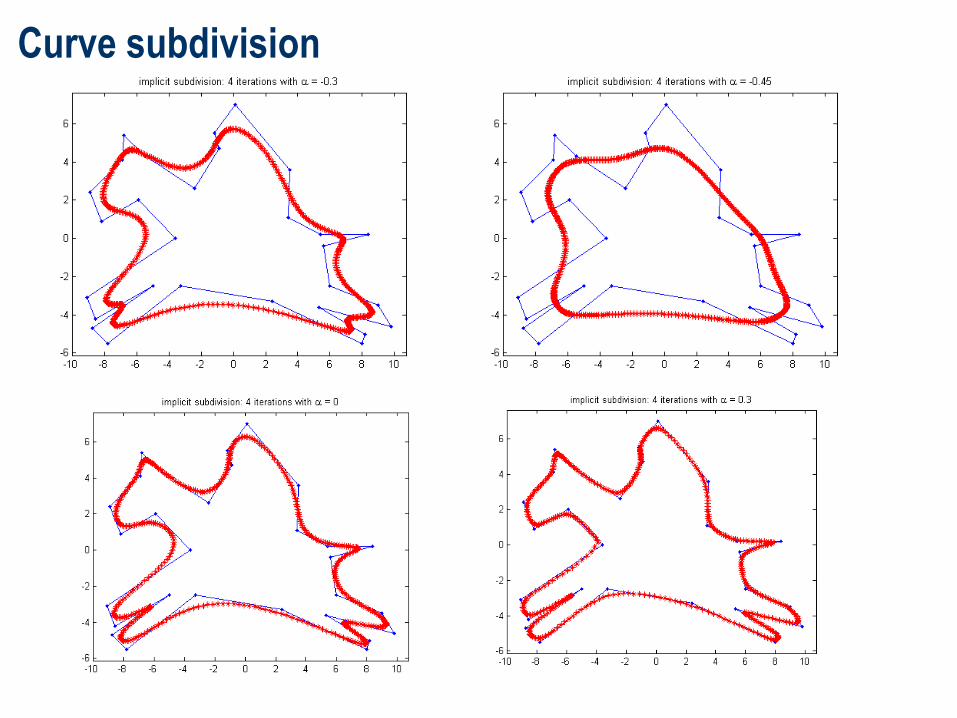
Curve subdivision
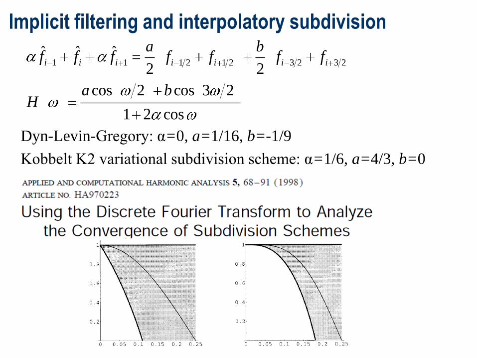
Implicit filtering and interpolatory subdivision
1 1 1 2 1 2 3 2 3 2ˆ ˆ ˆ
2 2
cos 2 cos 3 2
1 2 cos
i i i i i i i
a bf f f f f f f
a bH
Dyn-Levin-Gregory: α=0, a=1/16, b=-1/9
Kobbelt K2 variational subdivision scheme: α=1/6, a=4/3, b=0
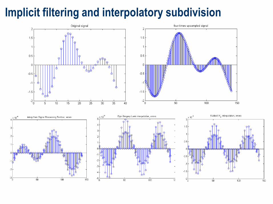
Implicit filtering and interpolatory subdivision

Implicit subdivision Implicit subdivision schemes were introduced by Kobbelt [1996,1998] in the
case of interpolatory subdivision from a variational standpoint.
Sabin [2010] does not mention them at all in his book (althought he cited that
paper of Kobbelt).
Peters and Reif [2008] devoted to variational subdivision only two sentences
where the authors acknowledged its existence but wrongly stated that more
or less nothing was known about the underlying theoretical properties of
variational subdivision schemes.

Future research
Weighted (non-iniform) implicit filtering schems edge-
aware image filtering (in a hope to beat results of Gastal &
Oliveira, Siggraph 2011).
Extending to mesh processing (in a hope to beat results of
Chuang & Kazhdan, Siggraph 2011).