Implicit-Explicit Numerical Methods in Models

of Cardiac Electrical Activity

By

Ryan C. Dean

Abstract

Mathematical models of electric activity in cardiac tissue are becoming an increasingly powerful

tool in the study of the heart and cardiac arrhythmias. The ordinary differential equations con-

tained within these mathematical models are challenging to solve. This challenge often means that

the physiological accuracy of a model is limited by how efficient we can make the numerical solution

process. In this thesis, we examine the efficiency of the numerical solution of four cardiac electro-

physiological models using Implicit-Explicit (IMEX) methods. We find that a particular IMEX

method, ARK5, can be up to 275 times faster than some methods most frequently used in practice.

i

Acknowledgements

I would like to thank Dr. Raymond Spiteri for all the time, encouragement, constructive criti-

cism, financial support, and effort he has given to myself and this project. This project would not

have been possible without him

I would also like to thank Mary MacLachlan and Sarah Healy for supplying Matlab code to help

debug the odeToJava code, and for some helpful comments along the way.

ii

Contents

Abstract i

Acknowledgements ii

Contents iii

List of Tables iv

List of Figures v

1 Introduction 1

2 Electrical Activity of the Heart 32.1 Relevant Background on the Heart . . . . . . . . . . . . . . . . . . . . . . . . . . . . 32.2 The Model of Luo and Rudy . . . . . . . . . . . . . . . . . . . . . . . . . . . . . . . 42.3 The Model of Courtemanche et al. . . . . . . . . . . . . . . . . . . . . . . . . . . . . 62.4 The Model of Winslow et al. . . . . . . . . . . . . . . . . . . . . . . . . . . . . . . . 62.5 The Model of Puglisi and Bers . . . . . . . . . . . . . . . . . . . . . . . . . . . . . . 7

3 Mathematical Background 83.1 Differential Equations . . . . . . . . . . . . . . . . . . . . . . . . . . . . . . . . . . . 83.2 Numerical Methods . . . . . . . . . . . . . . . . . . . . . . . . . . . . . . . . . . . . . 9

3.2.1 Basic Concepts . . . . . . . . . . . . . . . . . . . . . . . . . . . . . . . . . . . 93.2.2 Error and Stability . . . . . . . . . . . . . . . . . . . . . . . . . . . . . . . . . 113.2.3 Runge-Kutta Methods . . . . . . . . . . . . . . . . . . . . . . . . . . . . . . . 123.2.4 Implicit-Explicit Methods . . . . . . . . . . . . . . . . . . . . . . . . . . . . . 133.2.5 Implementation . . . . . . . . . . . . . . . . . . . . . . . . . . . . . . . . . . . 15

4 Results 164.1 Constant Step Size Tests . . . . . . . . . . . . . . . . . . . . . . . . . . . . . . . . . . 17

4.1.1 Explicit Runge-Kutta Methods . . . . . . . . . . . . . . . . . . . . . . . . . . 174.1.2 NSFD Method . . . . . . . . . . . . . . . . . . . . . . . . . . . . . . . . . . . 17

4.2 Variable Step Size Tests . . . . . . . . . . . . . . . . . . . . . . . . . . . . . . . . . . 174.3 Sparsity Patterns . . . . . . . . . . . . . . . . . . . . . . . . . . . . . . . . . . . . . . 214.4 Eigenvalues . . . . . . . . . . . . . . . . . . . . . . . . . . . . . . . . . . . . . . . . . 22

5 Conclusion 30

A Mathematical Models 33A.1 The Model of Luo-Rudy . . . . . . . . . . . . . . . . . . . . . . . . . . . . . . . . . . 33A.2 The Model of Courtemanche et al. . . . . . . . . . . . . . . . . . . . . . . . . . . . . 36A.3 The Model of Winslow et al. . . . . . . . . . . . . . . . . . . . . . . . . . . . . . . . 37A.4 The Model of Puglisi-Bers . . . . . . . . . . . . . . . . . . . . . . . . . . . . . . . . . 40

iii

List of Tables

4.1 Initial values for V . . . . . . . . . . . . . . . . . . . . . . . . . . . . . . . . . . . . . 164.2 ERK with Contant Step Size . . . . . . . . . . . . . . . . . . . . . . . . . . . . . . . 174.3 NSFD with Constant Step Size . . . . . . . . . . . . . . . . . . . . . . . . . . . . . . 184.4 Luo-Rudy Dormand Prince Results . . . . . . . . . . . . . . . . . . . . . . . . . . . . 184.5 Luo-Rudy ARK5 Results . . . . . . . . . . . . . . . . . . . . . . . . . . . . . . . . . 184.6 Courtemanche et al. Dormand-Prince Results . . . . . . . . . . . . . . . . . . . . . . 194.7 Courtemanche et al. ARK5 Results . . . . . . . . . . . . . . . . . . . . . . . . . . . . 194.8 Winslow et al. Dormand-Prince Results . . . . . . . . . . . . . . . . . . . . . . . . . 204.9 Winslow et al. ARK5 Results . . . . . . . . . . . . . . . . . . . . . . . . . . . . . . . 204.10 Puglisi-Bers ARK5 Results . . . . . . . . . . . . . . . . . . . . . . . . . . . . . . . . 214.11 Puglisi-Bers Dormand-Prince Results . . . . . . . . . . . . . . . . . . . . . . . . . . . 21

A.1 Parameters for the Luo-Rudy Phase I model . . . . . . . . . . . . . . . . . . . . . . . 36

iv

List of Figures

2.1 Transmembrane potential over time in the Luo-Rudy model. . . . . . . . . . . . . . . 5

3.1 Forward Euler . . . . . . . . . . . . . . . . . . . . . . . . . . . . . . . . . . . . . . . . 10

4.1 Sparsity pattern for the Jacobian of the Luo-Rudy model. . . . . . . . . . . . . . . . 224.2 Sparsity pattern for the Jacobian of the Courtemanche et al. model. . . . . . . . . . 234.3 Sparsity pattern for the Jacobian of the Winslow et al. model. . . . . . . . . . . . . 244.4 Sparsity pattern for the Jacobian of the Puglisi-Bers model. . . . . . . . . . . . . . . 254.5 Eigenvalues for the Jacobian of the Luo-Rudy model. . . . . . . . . . . . . . . . . . . 264.6 Eigenvalues for the Jacobian of the Courtemanche et al. model. . . . . . . . . . . . . 274.7 Eigenvalues of the Jacobian of the Winslow et al. model. . . . . . . . . . . . . . . . . 284.8 Eigenvalues for the Jacobian of the Puglisi-Bers model. . . . . . . . . . . . . . . . . . 29

v

Chapter 1

Introduction

Computer simulation is quickly becoming an important tool in cardiovascular research. Math-

ematical models of the heart can be used to simulate heart conditions and how certain drugs treat

these problems. The development of a drug often costs hundreds of millions of dollars [8]; computer

simulation aims to cut this cost by reducing the number of physical experiments needed in testing

a given drug.

Electrophysiological models of the heart describe how electricity flows through the heart, con-

trolling the contraction of the muscle. The models we consider consist of systems of ordinary

differential equations (ODEs). Cardiac electrophysiological models are often based on the Nobel

prize winning work of Hodgkin and Huxley [12] in the 1950s that modelled neural tissue mathe-

matically as a circuit. Modern cardiac electrophysiological models adapt the work of Hodgkin and

Huxley to describe electrical activity in the heart and include data gathered with from experiments

to form increasingly physiologically accurate models.

One of the major barriers to getting useful results from these simulations is the challenge of

performing the simulations efficiently. Sometimes the physiological accuracy of the mathematical

model must be reduced in the name of simplicity before we may perform the simulation efficiently

or even at all [11]. The ODEs found in these models are nonlinear and stiff. The consequence of

the stiffness is that the speed with which we can solve these ODEs is limited by stability instead

of accuracy. This limitation means that the solution process is much less efficient than it might

otherwise be.

In this thesis, we propose to improve the efficiency of the simulation process by using an Implicit-

Explicit (IMEX) numerical method [13]. An IMEX method approximates the solution of an ODE

which is split into two parts: one part better suited for an implicit numerical method and one

part better suited for an explicit numerical method. The IMEX solver uses both an implicit and

an explicit method to approximate the solution to the respective parts of the ODE. Using these

methods together, we are able to maximize the efficiency of the solution by using the better method

for each part. Cardiac electrophysiological models contain linear and nonlinear terms as well as stiff

and non-stiff terms, and so an IMEX method is a natural choice. Despite this, there is no published

work on the use of IMEX schemes as described in this thesis to solve cardiac electrophysiological

1

models.

In this thesis, we consider four mathematical models of cardiac electrophysiology: the Luo-

Rudy model of guinea pig ventricular tissue [17], the Courtemanche et al. model of human atrial

tissue [7], the Winslow et al. model of canine ventricular tissue [25], and the Puglisi-Bers model of

rabbit ventricular tissue [20]. In this thesis, we perform a rigorous comparison of an IMEX method,

ARK5 [15], to standard methods to solving these four models, and we then consider optimizations

to the IMEX process. The rest of the thesis is organized as follows. In Chapter 2 we give an

introduction to the physiology and mathematical models of electrical activity in the heart. In

Chapter 3 we give an introduction to ODEs and the numerical approximation to the solution of

ODEs. In Chapter 4 we discuss the results of the numerical experiments. In Chapter 5 we give a

summary of the results and discuss future work.

2

Chapter 2

Electrical Activity of the Heart

2.1 Relevant Background on the Heart

The heart is the muscle responsible for propelling blood throughout the body. A mammalian heart

consists of four connected chambers, two atria and two ventricles, guarded by valves [21]. The atria

receive and transfer blood to the ventricles. The ventricles then propel the blood outside of the

heart. Inside the right atrium is the sinoatrial node, which acts as the heart’s natural pacemaker.

In the lower right atrium is the atrioventricular node (AV node), which is connected to the bundle

of His. The heart contracts and relaxes on a regular cycle to pump blood into the lungs and body.

The heart muscle consists a large number of cells, every one of which has an electric potential.

At its resting potential, a cell is negatively charged with respect to its surroundings. A reversal in

membrane potential is called an action potential. This consists of several stages [21]. First there

is a rapid depolarization caused by the opening of fast sodium channels and closing of potassium

channels. This results in a short period of positive potential as the cell approaches equilibrium

potential for sodium. Calcium then enters through L-type calcium channels, and the cell is in

the plateau phase. During the plateau phase the cell remains depolarized so that the cell does

not relax again until all the blood has been pumped. Next potassium channels are reopened and

repolarization begins, causing the cell to return to resting potential. Finally, as the cell approaches

its equilibrium potential for potassium, the cell is again at resting potential, ready for another cycle.

Electrical activity is responsible for the contraction and relaxation of the heart. An action

potential is initiated spontaneously in specialized tissue inside the sinoatrial node [9]. Electrical

activity spreads from one cell to another via areas of low resistance between them known as gap

junctions. As the action potential reaches an individual cell, the result is a powerful force develop-

ment and/or mechanical shortening. Action potentials first spread over the atria causing them to

contract, transferring blood to the ventricles. Next the action potentials reach the AV node. The

AV node spreads the action potential to the ventricles but delays it enough to allow the ventricles

to fill completely.

Many heart problems are the result of irregularities in the flow of electricity in the heart.

Abnormal electrical activity is called an arrhythmia, which in general is caused either by abnormal

3

impulse formation or re-entry [23]. Re-entry is the result of an electrical impulse that persists

past the normal activation of the heart and re-excites tissue that has already contracted during

the current heartbeat. This causes irregularities in the heartbeat that can lead to many serious

problems, including death. To be able to study these conditions noninvasively is one common

practical motivation for creating mathematical models of electrical activity in cardiac tissue.

The specific objective of these mathematical models is to model the heart and heart conditions

in order to simulate treatments; i.e., we can use these mathematical models to perform computer

simulations of the effects of new drugs to treat these heart conditions. The development of a

new drug has an average cost of approximately $900 million [8]; one objective of using computer

simulation to simulate new drugs is to reduce the number of physical experiments needed to develop

the drug and therefore reduce this cost. As the models become more physiologically accurate we

are able to obtain more useful information from these simulations.

Obtaining physiologically accurate mathematical models is a difficult task. A major barrier

to obtaining physiological accuracy is the challenging task of performing the simulation efficiently.

One reason producing an efficient simulation is difficult is that the mathematical models are quite

intricate. This means we must perform a large number of computations when evaluating the

right hand side of the ODE1. Another challenge to performing efficient simulations is that the

mathematical models are numerically stiff, and so we must use sophisticated numerical methods

to perform these simulations efficiently. The two challenges described above are amplified when

we move from a model for one cell to a model of many cells in two or three dimensions. To move

effectively beyond models for one cell, we need to include enough cells in our model to realistically

approximate the geometry and physiology of the heart. Because the heart has more than two

billion cells, any realistic simulation will have enough cells to magnify any inefficiencies in the

numerical dramatically, possibly even hundreds of thousands of times. The difficulty posed by

these challenges has caused some researchers to reduce the physiological accuracy of their model

to allow the simulation to be performed within an acceptable amount of time [11]. If we are able

to significantly improve the efficiency of the simulation process, then we can gain physiological

accuracy in our model and therefore perform more realistic simulations.

2.2 The Model of Luo and Rudy

In 1991 Ching-Hsing Luo and Yoram Rudy developed a model2 of guinea pig ventricular action

potentials based on a previous model from Beeler and Rueter [4]. The Luo-Rudy model [17]

extended the Beeler-Reuter model to include fast inward sodium and outward potassium currents

1See Chapter 3 for a discussion of the mathematical concepts used in this paragraph.2See Chapter 3 for a discussion of the mathematics contained within this model.

4

0 50 100 150 200 250 300 350 400 450−100

−50

0

50Voltage

Time (ms)

Vol

tage

(mV

)

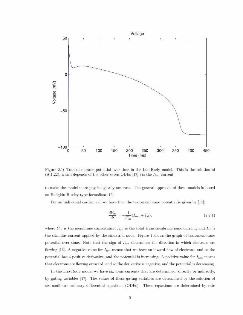
Figure 2.1: Transmembrane potential over time in the Luo-Rudy model. This is the solution of(A.1.22), which depends of the other seven ODEs [17] via the Iion current.

to make the model more physiologically accurate. The general approach of these models is based

on Hodgkin-Huxley-type formalism [12].

For an individual cardiac cell we have that the transmembrane potential is given by [17]:

dVmdt

= − 1

Cm(Iion + Ist), (2.2.1)

where Cm is the membrane capacitance, Iion is the total transmembrane ionic current, and Ist is

the stimulus current applied by the sinoatrial node. Figure 1 shows the graph of transmembrane

potential over time. Note that the sign of Iion determines the direction in which electrons are

flowing [16]. A negative value for Iion means that we have an inward flow of electrons, and so the

potential has a positive derivative, and the potential is increasing. A positive value for Iion means

that electrons are flowing outward, and so the derivative is negative, and the potential is decreasing.

In the Luo-Rudy model we have six ionic currents that are determined, directly or indirectly,

by gating variables [17]. The values of these gating variables are determined by the solution of

six nonlinear ordinary differential equations (ODEs). These equations are determined by rate

5

parameters αy and βy, where y is any gating variable. These equations take the general form:

dy

dt=y∞ − yτy

, (2.2.2)

where

y∞ =αy

αy + βy, (2.2.3)

τy =1

αy + βy. (2.2.4)

The remaining ODE in the Luo-Rudy model describes calcium concentration in the cell:

d ([Ca]i)

dt= −10−4Isi + 0.07(10−4 − [Ca]i), (2.2.5)

where [Ca]i is the intracellular calcium concentration, and Isi is the slow inward calcium current [17].

The six gating equations of the form (A.1.22) are coupled with (2.2.2) and (2.2.5) to form the

complete Luo-Rudy model.

See section A.1 for a complete listing of the Luo-Rudy model.

In 1994 Luo and Rudy published an improvement to this model, now known as the Luo-Rudy

Phase II model [18, 19]. This model gives a more accurate physiological model by including the

actions of ionic pumps and changes in ionic concentrations.

2.3 The Model of Courtemanche et al.

In 1998 Marc Courtemanche, Rafael Ramirez, and Stanley Nattel developed a model of human

atrial action potentials [7]. This model was a response to new findings that show there are some

important differences in human action potentials when compared to other mammals frequently used

in models and tests. Courtemanche et al. developed this model with human data and supplemented

it with animal data when needed. The Courtemanche et al. model is an extension of the Luo-Rudy

Phase II model. It consists of 21 ODEs, which are listed in section A.2.

2.4 The Model of Winslow et al.

In 1999 Raimond Winslow, Jeremy Rice, Saleet Jafri, Eduardo Marbn, and Brian O’Rourke de-

veloped a model of canine ventricular tissue [25]. This model is based on a guinea pig model that

was an extension of the Luo-Rudy Phase II model. The Winslow et al. model was developed using

experimental data to modify the guinea pig model so that it would simulate canine ventricular

tissue. The canine heart is more similar to a human heart than a guinea pig heart, and there are

6

more canine heart data than human heart data available. The Winslow et al. model is particularly

detailed when describing the dynamics of Ca2+, which is an important consideration in heart fail-

ure. The Winslow et al. model consists 32 ODEs, listed in section A.3, making it the most complex

of the models in this study.

2.5 The Model of Puglisi and Bers

In 2001 Jose Puglisi and Donald Bers developed a model of rabbit ventricular tissue [20]. Although

rabbit ventricular tissue is used frequently in physical experiments, no mathematical model had

been previously developed for it. This model was adapted from the Luo-Rudy model to include data

from the literature and from the joint laboratory of Puglisi and Bers. Much of the emphasis in this

model was placed on the user interface as this was designed to be a learning aid for students. The

convenient user interface was designed also as a tool for researchers to reproduce experimental and

physical results on the computer. Thus, physiological accuracy is also of paramount importance.

Puglisi and Bers give particular detail to calcium handling so that the model can accurately simulate

heart failure. This model contains 17 ODEs. This model is also referred to as the LabHeart [20]

model. See A.4 for a complete listing of equations.

7

Chapter 3

Mathematical Background

3.1 Differential Equations

The material is this section is largely adapted from [6].

A differential equation is an equation that contains an unknown function and its derivatives. If

the unknown function y depends only on to one independent variable t, then the equation

F(t,y,y′, ...,y(n)

)= 0. (3.1.1)

is called an ordinary differential equation (ODE). In this study we are primarily concerned with

ODEs of the form:dy

dt= f (t,y) .

That is, we are looking at equations that describe the rate of change of y over time.

Sometimes we may need more than one independent variable to mathematical model a given

process. For example, modelling heat flow through a metal rod requires independent variables in

both time and space. If we have more than one independent variable, then we may take a derivative

with respect to any one of the independent variables while treating the other independent variables

as constants. This is called a partial derivative. If a differential equation contains a partial derivative

of an unknown function of more than one independent variable, it is called a partial differential

equation.

A solution of the ODE (3.1.1) is a function with n derivatives that satisfies (3.1.1). When we

have known initial values for a function and n−1 of its derivatives we have an initial value problem

(IVP). This initial value problem usually gives us a specific solution to an ODE, as opposed to a

general solution that will contain arbitrary constants of integration.

The theory of ODEs is both rich and verbose, but here we only list one result that is of impor-

tance in our study:

Theorem 3.1.1. (Existence and Uniqueness) Consider the initial value problem:

y′(t) = f (t,y(t)) .

8

y(0) = y0.

Let f be continuous for all (t,y) in D:

D = {0 ≤ t ≤ b,−∞ < ||y|| <∞}.

Let f satisfy a Lipschitz condition for all (t,y) in D:

||f(t,y) − f(t,y∗)|| ≤ L||y − y∗||

for some constant 0 < L < ∞ and all t,y,y∗ in D. Then for any y0 there exists a unique and

differentiable solution to the ODE in [0, b].

3.2 Numerical Methods

3.2.1 Basic Concepts

The material in subsections 3.2.1, 3.2.2, and 3.2.3 has been mainly adapted from [22] and [14].

Although analytical methods exist to solve differential equations, we are often faced with a dif-

ferential equation that cannot be solved analytically. Differential equations or systems of differential

equations that model problems in all of the mathematical sciences are often large, complicated, and

nonlinear. When analytical methods are unavailable, one may use numerical methods to approxi-

mate the solution to a differential equation.

The simplest numerical method for approximating the solution of an IVP is Euler’s method, also

known as Forward Euler. Euler’s method approximates the solution of the initial value problem

dy

dt= f (t,y) ,y(0) = y0,

on the interval [0, b]. One step of Euler’s method is given by

yn = yn−1 + ∆tnf (tn−1,yn−1) ,

tn = tn−1 + ∆tn.

Each step approximates the solution at time tn. Note that ∆tn need not be constant. Recalling

that the slope of the tangent line at time t for y(t) is given by

y′(t) = f (t,y(t)) ,

we can see that Forward Euler is an approximation of the tangent line at each interval. See Figure

9

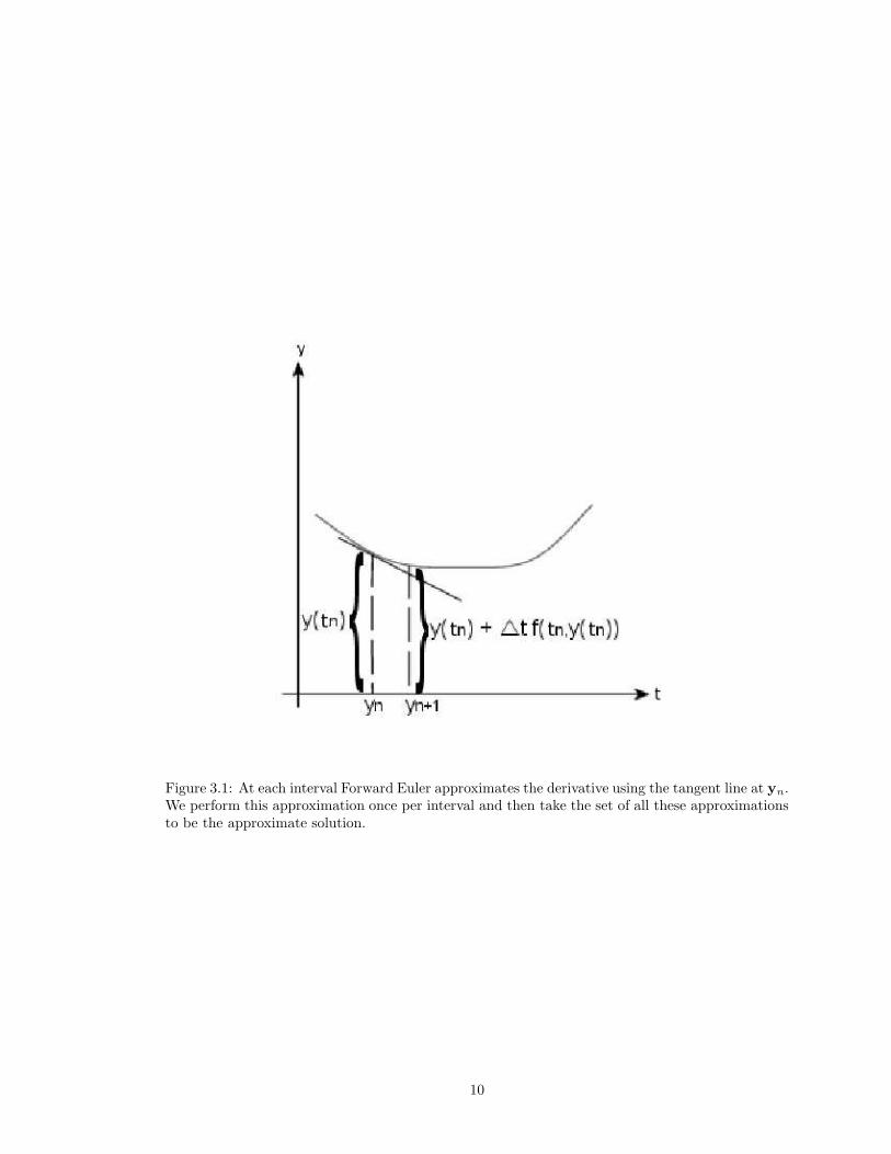
Figure 3.1: At each interval Forward Euler approximates the derivative using the tangent line at yn.We perform this approximation once per interval and then take the set of all these approximationsto be the approximate solution.

10

3.1. That is, geometrically, the approximate solution produced by Forward Euler is the union of

each of these approximations over the entire solution interval. So, in theory, as ∆t approaches zero,

the approximation given by Forward Euler approaches the true solution. In other words, given

infinite precision, Forward Euler’s approximation converges to the true solution as ∆t approaches

zero, but in practice we are limited by the finite amount of precision available on a given computer.

This notion of convergence is very important when discussing numerical methods. Each numer-

ical method has an order of convergence. We say a method is of order p if

yn − y(tn) = O(∆tp+1). (3.2.1)

It can be shown that Forward Euler is of order 1 [22], which is a lower order of convergence than

we generally would like to have in practice.

3.2.2 Error and Stability

No matter how sound the numerical method used, the approximation process naturally produces

some error. For example, we introduce error when we discretize our continuous equation, and further

error is introduced when the solution is computed with finite precision. To obtain an acceptable

approximation a numerical method must limit all sources of error. One method to control the error

is to estimate the error at each time step and then, if necessary, adjust the size of the step. If the

error is too large, the step is rejected, and the solver will try again using a smaller step size. If

the error is much smaller than necessary the solver can increase the size of the next step and thus

increase efficiency.

If the stepsize used is too large, then the approximation process generally becomes unstable.

If the choice of step size of an approximation is determined by stability rather than accuracy,

then the ODE is said to be stiff 1. Generally, the step size required for a stiff problem is much

smaller than accuracy requirements would dictate; for efficiency purposes we want to be able to

choose a method based only the accuracy requirements. We can understand this to some extent by

considering absolute stability theory.

In absolute stability theory we consider the numerical approximation of the solution of

y′ = λy, t ≥ 0, y(0) = y0, λ ∈ C,

with a given numerical method. The analytical solution of this equation is

y(t) = y0eλt, (3.2.2)

1Arguably, the definition of a stiff problem is not entirely universal, but this description of stiffness suffices forour study.

11

and so we have

limt→∞

|yn| → 0 (3.2.3)

if and only if

Re(λ) ≤ 0.

We say the region of absolute stability of the given numerical method is the set of all λ∆t ∈ Csuch that (3.2.3) holds and ||yn+1|| ≤ ||yn||. It is for these λ∆t the method is absolutely stable. A

special case is when the region of absolute stability contains the left hand side of the complex plane.

Methods with this property are called A-stable. With A-stable methods we have no restrictions on

∆t due to stability (at least for the model problem (3.2.2)), and hence they are a good choice for

stiff methods.

If the numerical method is able to produce a stable approximation we are then interested in how

close the approximation is to the true solution. When the true solution is known, this is simple: we

can simply compare the two. Otherwise, we must make an estimate. In order to make an estimate

on the error in the approximation, we generate a reference solution by lowering the error tolerance

until we produce two approximations that are identical within a desired number of significant digits.

We can then compare the approximation, Y, to the reference solution, Y. A popular way to do

this in the literature on heart simulation is the Relative Root Mean Squared (RRMS) error :

RRMS =

√√√√∑Ni=1(Yi − Y)2

2∑Ni=1 Y2

i

,

where Yi = Y(ti) and Yi = Y(ti) are the numerical approximations at time ti ∈ [0, b], i =

1, 2, . . . , N .

In biomedical research 5% RRMS error is considered acceptable; our goal is, therefore, to

produce the most efficient solution we can with 5% or less RRMS error.

3.2.3 Runge-Kutta Methods

A general class of numerical methods for solving ODEs is called Runge-Kutta methods [14]. Euler’s

method is the simplest of this class of methods. We aim to improve on Euler’s method by improving

the order of convergence and hence the accuracy of our approximation. A general s-stage Runge-

Kutta method has the form:

ki = f

tn−1 + ∆tci,yn−1 + ∆t

s∑

j=1

aijkj

, i = 1, 2, ..., s,

12

yn = yn−1 + ∆t

s∑

i=1

biki.

These equations can be summarized by means of the Butcher Tableau [14]:

c1 a11 a12 ... a1s

c2 a21 a22 ... a2s

......

.... . .

...

cs as1 as2 ... ass

b1 b2 ... bs

or

c A

bT

A Runge-Kutta method is explicit if A is strictly lower triangular and implicit if any aij on or

above the diagonal is non-zero. Implicit Runge-Kutta methods are useful for stiff problems [14].

The choice of parameters for a specific Runge-Kutta method is often made based on desired

order requirements. In other words, we try to pick terms such that the truncation error is of a

certain order. The idea is that repeated function evaluations are used to eliminate lower order

truncation error terms. An example of a higher order method is the classical Runge-Kutta method,

denoted by ERK4:

0 0 0 0 0

12

12 0 0 0

12 0 1

2 0 0

1 0 0 1 0

16

13

13

16

This is a four stage, fourth order explicit Runge-Kutta method.

3.2.4 Implicit-Explicit Methods

When solving ODEs numerically we may find the ODE can be separated into two parts:

dy

dt= f (t,y) + g (t,y) ,

where f(t,y) is most efficiently approximated with one method and g(t,y) is most efficiently ap-

proximated with another method. In such cases, particularly when the efficient method for one

part is inefficient for the other, a splitting technique may be used to obtain an approximation effi-

ciently for the whole equation [13]. Here we break the approximation into two parts and use the

appropriate method for each part of the equation.

13

In particular, if f(t,y) is such that it is best approximated with an explicit method and g(t,y) is

such that it is best approximated with an implicit method, we may use an Implicit-Explicit (IMEX)

method to approximate the solution to this equation efficiently [13]. An example of when an IMEX

method would be useful is when f(t,y) consists of non-stiff and/or nonlinear terms and that g(t,y)

consists of stiff and/or linear terms.

As an example [3] we can look at the combination of Forward and Backward Euler, given by

the respective Butcher Tableaux:

1 1

1

0 0

1

which when padded, to simplify the form of the order conditions, become:

0 0 0

1 0 1

0 1

0 0 0

1 1 0

1 0

This gives the following IMEX method:

yn = yn−1 + ∆t (f (yn−1) + g (yn)) .

In a more general sense we are considering an s-stage implicit method with coefficients A, c,b in

the usual Butcher notation with an (s+ 1)-stage explicit method with coefficients A, b, c. Here we

have c = (0 c)T . Let σ = s+ 1. One step of the IMEX method is given by [3]:

Set

K1 = f(yn−1).

Then for i = 1, ..., s:

• Solve for Ki

Ki = g (yi) .

where

yi = yn−1 + ∆t

i∑

j=1

aijKj +

i∑

j=1

ai+1,jKj .

• Evaluate

Ki+1 = f (yi) .

Finally, evaluate

yn = yn−1 + ∆ts∑

j=1

bjKj +σ∑

j=1

bjKj .

14

See [3] for further details.

This thesis considers the numerical method ARK5(3)8L[2]SA, also known as ARK5 [15], as an

alternative to standard methods used to approximate the solution to cardiac electrophysiological

models. ARK5 is a 2-additive Runge-Kutta method of order 5(4) with eight stages. In general, an

n-additive embedded Runge-Kutta method consists of n Runge-Kutta methods to solve n different

parts of the ODE. ARK5 uses two Runge-Kutta methods, one explicit and one implicit, and so it

is an IMEX method that uses the procedure described in this section to take a step. The Butcher

tableaux of ARK5 are listed in [15].

3.2.5 Implementation

All four models were implemented in odeToJava [2], a Java based initial value problem solving

environment. Using odeToJava we performed numerical experiments using Forward Euler, ERK4,

Dormand-Prince 5(4), and ARK5 and compared their performance.

Matlab implementations of the Luo-Rudy, Courtemanche et al., and Winslow et al. models

were written by Mary MacLachlan, and a Matlab implementation of the Puglisi-Bers model was

written by Sarah Healy. The Matlab code was used to verify that the odeToJava code had been

implemented correctly and to verify results obtained using the odeToJava code. For example,

the maximum stable step size of Forward Euler should be the same for both the Matlab and

odeToJava code and any discrepancy is evidence of a bug. The Matlab code was also used to gain

useful information using specialized Matlab routines. For example, Matlab’s spy routine was used

to produce the figures in Section 4.3, as there is no such feature in odeToJava.

The mathematical models were also partially implemented in Maple. This was also done to

verify that the odeToJava code was implemented properly. Maple is a useful tool to perform such

a task as it obtains results symbolically instead of numerically; one advantage of this is that we

may avoid making the same mistake in both implementations because we are forced to use a very

different process to obtain results.

15

Chapter 4

Results

After the models were implemented, their solutions were approximated with a variety of nu-

merical methods. This chapter lists the results of the comparisons of these numerical methods.

We approximated the solution of the four cardiac electrophysiological models using the IVP solvers

described in Chapter 3. As an initial value we use, with the exception of voltage, the values of all

variables while the heart is in its resting state. In some models, initial value for voltage was altered

to account for the current from the sinoatrial node. The discontinuous nature of the current from

the sinoatrial node can cause numerical problems; we alter the alter the initial value of the voltage

such that we remove this numerical problem yet maintain physiological accuracy. The initial values

we use for voltage in each one of the models are listed in Table 4.1. See [17], [7], [25], [20] for

complete listings of the initial values.

The models were solved over a time interval that represents one cardiac cycle. The Luo-Rudy

model was considered on the interval [0,450] milliseconds, the Courtemanche et al. model was

considered on the interval [0,500] milliseconds, the Winslow et al. model was considered on the

interval [0,300] milliseconds, and the Puglisi-Bers model was considered on the interval [0,330]

milliseconds. The different solution intervals are due to different physiological properties of the

specific mammalian heart that the model represents.

Model VrestLuo-Rudy -35

Coutemanche et al. -81.2Winslow et al. -35Puglisi-Bers -85.5

Table 4.1: Initial values for V = Vrest

16

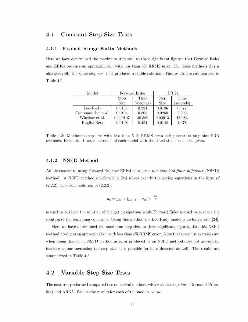
4.1 Constant Step Size Tests

4.1.1 Explicit Runge-Kutta Methods

Here we have determined the maximum step size, to three significant figures, that Forward Euler

and ERK4 produce an approximation with less than 5% RRMS error. For these methods this is

also generally the same step size that produces a stable solution. The results are summarized in

Table 4.2.

Model Forward Euler ERK4Step Time Step TimeSize (seconds) Size (seconds)

Luo-Rudy 0.0134 0.224 0.0186 0.677Coutemanche et al. 0.0194 0.805 0.0268 2.292

Winslow et al. 0.000107 40.369 0.00013 130.83Puglisi-Bers 0.0108 0.454 0.0148 1.078

Table 4.2: Maximum step size with less than 5 % RRMS error using constant step size ERKmethods. Execution time, in seconds, of each model with the listed step size is also given.

4.1.2 NSFD Method

An alternative to using Forward Euler or ERK4 is to use a non-standard finite difference (NSFD)

method. A NSFD method developed in [24] solves exactly the gating equations in the form of

(2.2.2). The exact solution of (2.2.2),

yn = y∞ + (yn−1 − y∞)e−∆tτy ,

is used to advance the solution of the gating equation while Forward Euler is used to advance the

solution of the remaining equations. Using this method the Luo-Rudy model is no longer stiff [24].

Here we have determined the maximum step size, to three significant figures, that this NSFD

method produces an approximation with less than 5% RRMS error. Note that one must exercise care

when doing this for an NSFD method as error produced by an NSFD method does not necessarily

increase as one increasing the step size; it is possible for it to decrease as well. The results are

summarized in Table 4.3

4.2 Variable Step Size Tests

The next test performed compared two numerical methods with variable step sizes: Dormand-Prince

5(4) and ARK5. We list the results for each of the models below.

17

Model Max Step Size TimeLuo-Rudy 0.250 0.046

Coutemanche et al. 0.345 0.081Winslow et al. 0.00028 57.32Puglisi-Bers 0.43 0.066

Table 4.3: Maximum step size with less than 5 % error using constant step size using an NSFDmethod.

rtol = atol = (1× 10i) RRMS Error Time(seconds) Average Step Size-12 5.198E-14 20.29 2.150E-2-11 4.917E-14 1.316 3.157E-2-10 4.154E-14 0.946 4.410E-2-9 3.6164E-14 0.611 7.0104E-2-8 5.9490E-13 0.551 7.8933E-2-7 8.8183E-12 0.539 8.4065E-2-6 1.4975E-10 0.514 8.6455E-2-5 3.2922E-09 0.529 8.7327E-2-4 9.6103E-08 0.516 8.7531E-2-3 7.1231E-05 0.538 8.7599E-2-2 0.0170 0.52 9.2573E-2

Table 4.4: Luo-Rudy Dormand-Prince variable step size results.

rtol = RRMS Error Time Averageatol= (seconds) Step Size

1× 10i

-13 4.2557E-7 6.048 1.6865E-3-12 4.3221E-7 3.603 5.4534E-3-11 4.6300E-7 2.801 1.8703E-2-10 6.4571E-7 1.164 6.5607E-2-9 1.2386E-6 0.583 1.9728E-1-8 1.6158E-6 0.253 4.8859E-1-7 2.4671E-6 0.118. 1.178-6 5.0677E-6 0.069 2.486-5 1.9600E-6 0.048 4.945-4 2.6724E-5 0.038 8.333-3 1.1127E-4 0.034 11.53-2 1.000E-3 0.032 15.00

Table 4.5: Luo-Rudy ARK5 variable step size results.

18

The results for the Luo-Rudy model are listed in Tables 4.4 and 4.5. With Dormand-Prince

the execution time is approximately constant for all numerical approximations with an acceptable

amount of error; relaxing the error tolerance offers no significant improvement in execution time.

This is a telltale sign of stiffness in the Luo-Rudy model. With ARK5 we can always produce a

solution well within the maximum RRMS error, and we see a clear improvement in execution time

when we relax the error tolerance. Using ARK5 as the numerical method for the Luo-Rudy model

can produce an acceptable solution nearly 20 times faster than Dormand-Prince.

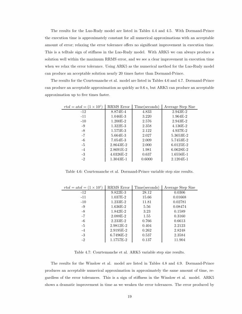
The results for the Courtemanche et al. model are listed in Tables 4.6 and 4.7. Dormand-Prince

can produce an acceptable approximation as quickly as 0.6 s, but ARK5 can produce an acceptable

approximation up to five times faster.

rtol = atol = (1× 10i) RRMS Error Time(seconds) Average Step Size-12 8.874E-4 4.833 2.943E-2-11 1.046E-3 3.220 1.964E-2-10 1.200E-2 2.576 2.943E-2-9 1.322E-3 2.358 4.136E-2-8 1.575E-3 2.122 4.937E-2-7 5.664E-3 2.027 5.3653E-2-6 7.054E-3 2.009 5.7453E-2-5 2.8643E-2 2.000 6.0125E-2-4 2.8691E-2 1.981 6.0628E-2-3 4.0326E-2 0.637 1.6556E-1-2 1.3043E-1 0.6000 2.1204E-1

Table 4.6: Courtemanche et al. Dormand-Prince variable step size results.

rtol = atol = (1× 10i) RRMS Error Time(seconds) Average Step Size-12 9.822E-3 28.12 0.0306-11 1.037E-2 15.66 0.01668-10 1.233E-2 11.81 0.02781-9 1.636E-2 5.56 0.08474-8 1.842E-2 3.23 0.1589-7 2.088E-2 1.55 0.3160-6 2.233E-2 0.766 0.6613-5 2.9812E-2 0.404 2.2123-4 2.9195E-2 0.262 2.8248-3 6.7496E-2 0.537 2.3584-2 1.1757E-2 0.137 11.904

Table 4.7: Courtemanche et al. ARK5 variable step size results.

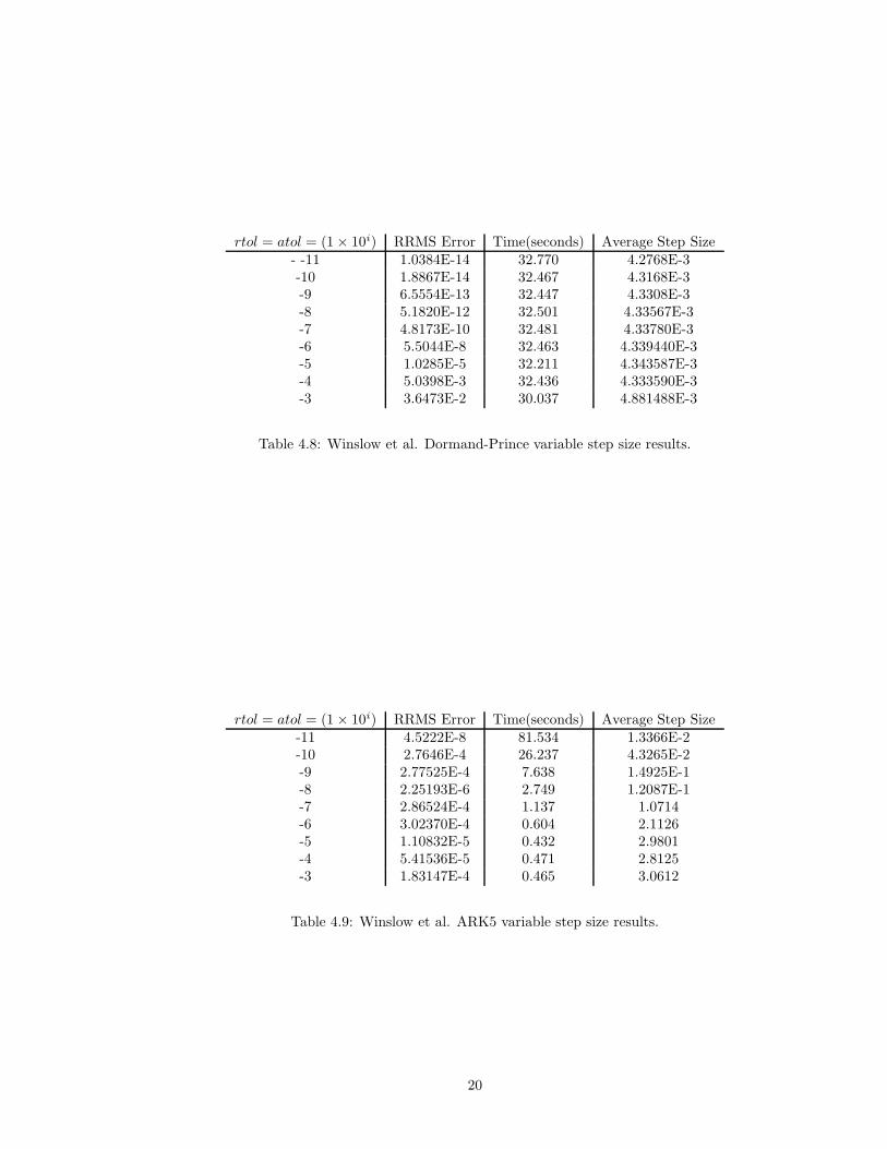
The results for the Winslow et al. model are listed in Tables 4.8 and 4.9. Dormand-Prince

produces an acceptable numerical approximation in approximately the same amount of time, re-

gardless of the error tolerances. This is a sign of stiffness in the Winslow et al. model. ARK5

shows a dramatic improvement in time as we weaken the error tolerances. The error produced by

19

rtol = atol = (1× 10i) RRMS Error Time(seconds) Average Step Size- -11 1.0384E-14 32.770 4.2768E-3-10 1.8867E-14 32.467 4.3168E-3-9 6.5554E-13 32.447 4.3308E-3-8 5.1820E-12 32.501 4.33567E-3-7 4.8173E-10 32.481 4.33780E-3-6 5.5044E-8 32.463 4.339440E-3-5 1.0285E-5 32.211 4.343587E-3-4 5.0398E-3 32.436 4.333590E-3-3 3.6473E-2 30.037 4.881488E-3

Table 4.8: Winslow et al. Dormand-Prince variable step size results.

rtol = atol = (1× 10i) RRMS Error Time(seconds) Average Step Size-11 4.5222E-8 81.534 1.3366E-2-10 2.7646E-4 26.237 4.3265E-2-9 2.77525E-4 7.638 1.4925E-1-8 2.25193E-6 2.749 1.2087E-1-7 2.86524E-4 1.137 1.0714-6 3.02370E-4 0.604 2.1126-5 1.10832E-5 0.432 2.9801-4 5.41536E-5 0.471 2.8125-3 1.83147E-4 0.465 3.0612

Table 4.9: Winslow et al. ARK5 variable step size results.

20

ARK5 behaves erratically, but we can produce an approximation within the desired RRMS error

in 0.465 seconds. For the model of Winslow et al. ARK5 is approximately up to 70 times faster

than Dormand-Prince.

rtol = atol = (1× 10i) RRMS Error Time(seconds) Average Step Size-13 8.46E-4 18.884 0.01644-12 6.33E-4 10.9 0.02904-11 4.22E-4 6.066 0.05182-10 3.65E-4 3.185 0.09906-9 3.18E-3 1.593 0.19400-8 1.15E-3 0.0803 0.37078-7 8.48E-3 0.0411 0.70663-6 0.057 0.0261 1.1224-5 9.96E-3 0.0201 0.7236-4 9.21E-3 0.0180 1.2132-3 1.578 0.0112 1.4798-2 0.118 0.0163 0.0871

Table 4.10: The results of numerical solutions of the Puglisi-Bers using the IMEX method ARK5with variable step sizes.

rtol = atol = (1× 10i) RRMS Error Time(seconds) Average Step Size-13 1.20E-4 3.582 0.01503-12 1.37E-4 2.821 0.01960-11 1.69E-4 2.382 0.02365-10 1.75E-4 2.106 0.02695-9 1.45E-4 1.996 0.02928-8 1.05E-4 1.885 0.03072-7 1.08E-4 1.843 0.03157-6 1.34E-4 1.823 0.03199-5 2.177E-4 1.812 0.03219-4 3.25E-4 1.809 0.03228-3 1.112E-3 1.804 0.03231-2 0.0303 1.525 0.04092

Table 4.11: The results of numerical solutions of the Puglisi-Bers using Dormand-Prince withvariable step sizes.

The results for the Puglisi-Bers model are listed in Tables 4.10 and 4.11. We find that ARK5

can produce an acceptable result up to 84 times faster than Dormand-Prince.

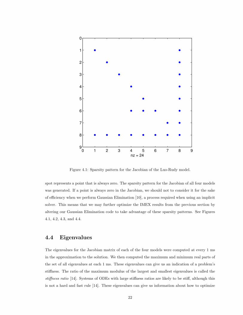
4.3 Sparsity Patterns

A sparsity pattern can be thought of as a map of a matrix: it describes which entries of a matrix are

always zero and which entries can be non-zero; in our case this is across the entire solution interval

of an ODE. A blue dot in the sparsity pattern represents a point that can be non-zero and a blank

21

0 1 2 3 4 5 6 7 8 9

0

1

2

3

4

5

6

7

8

9

nz = 24

Figure 4.1: Sparsity pattern for the Jacobian of the Luo-Rudy model.

spot represents a point that is always zero. The sparsity pattern for the Jacobian of all four models

was generated. If a point is always zero in the Jacobian, we should not to consider it for the sake

of efficiency when we perform Gaussian Elimination [10], a process required when using an implicit

solver. This means that we may further optimize the IMEX results from the previous section by

altering our Gaussian Elimination code to take advantage of these sparsity patterns. See Figures

4.1, 4.2, 4.3, and 4.4.

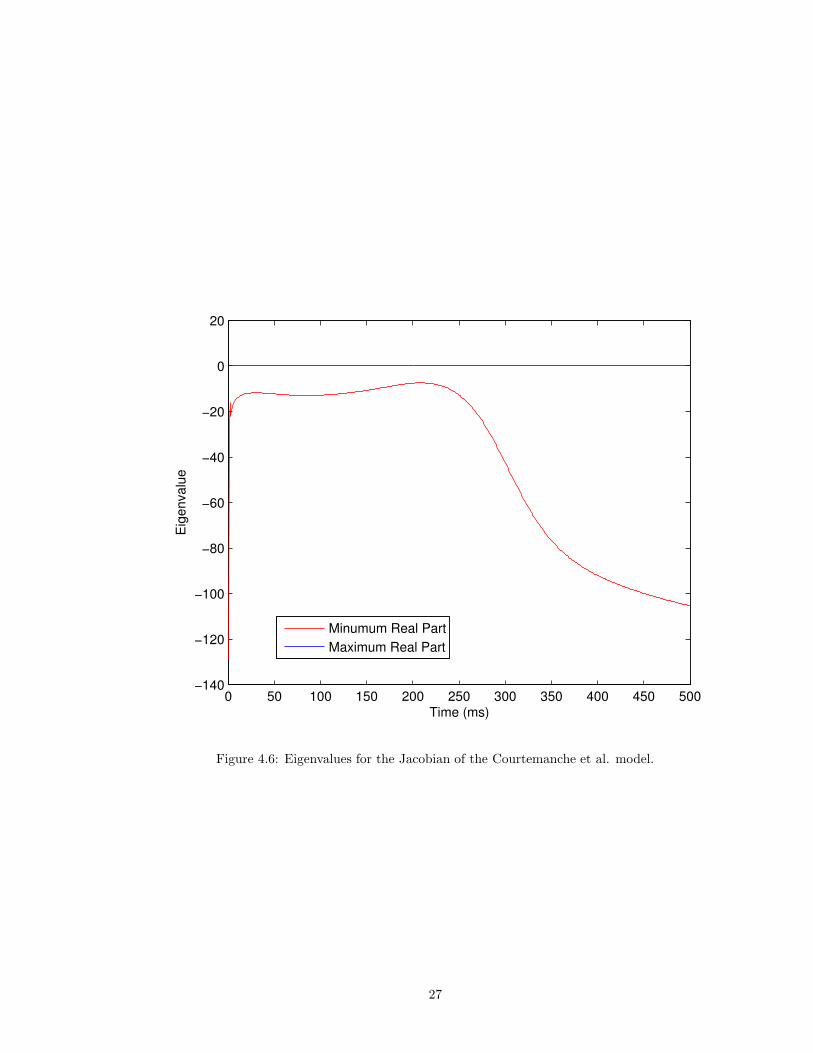
4.4 Eigenvalues

The eigenvalues for the Jacobian matrix of each of the four models were computed at every 1 ms

in the approximation to the solution. We then computed the maximum and minimum real parts of

the set of all eigenvalues at each 1 ms. These eigenvalues can give us an indication of a problem’s

stiffness. The ratio of the maximum modulus of the largest and smallest eigenvalues is called the

stiffness ratio [14]. Systems of ODEs with large stiffness ratios are likely to be stiff, although this

is not a hard and fast rule [14]. These eigenvalues can give us information about how to optimize

22

0 5 10 15 20

0

2

4

6

8

10

12

14

16

18

20

22

nz = 97

Figure 4.2: Sparsity pattern for the Jacobian of the Courtemanche et al. model.

23

0 5 10 15 20 25 30

0

5

10

15

20

25

30

nz = 134

Figure 4.3: Sparsity pattern for the Jacobian of the Winslow et al. model.

24

Figure 4.4: Sparsity pattern for the Jacobian of the Puglisi-Bers model.

25

0 50 100 150 200 250 300 350 400 450−160

−140

−120

−100

−80

−60

−40

−20

0

20

Time (ms)

Eig

enva

lue

Minimum Real PartMaximum Real Part

Figure 4.5: Eigenvalues for the Jacobian of the Luo-Rudy model.

the IMEX method. The results are displayed in Figures 4.5, 4.6, 4.7, and 4.8.

26

0 50 100 150 200 250 300 350 400 450 500−140

−120

−100

−80

−60

−40

−20

0

20

Time (ms)

Eig

enva

lue

Minumum Real PartMaximum Real Part

Figure 4.6: Eigenvalues for the Jacobian of the Courtemanche et al. model.

27

0 50 100 150 200 250 300−20000

−15000

−10000

−5000

0

5000

Time (ms)

Eig

enva

lues

Minimum Real EigenvalueMaximum Real Eigenvalue

Figure 4.7: Eigenvalues of the Jacobian of the Winslow et al. model.

28

0 50 100 150 200 250 300 350−200

−150

−100

−50

0

50

Figure 4.8: Eigenvalues for the Jacobian of the Puglisi-Bers model.

29

Chapter 5

Conclusion

In this thesis we considered the numerical approximation of solutions ODEs found in cardiac elec-

trophysiological models. In particular, we compared the efficiency of IMEX methods for performing

the numerical approximation to the solution of the ODEs found in four different electrophysiological

models to standard numerical methods. When comparing the IMEX method ARK5 to Forward

Euler, the results indicate that ARK5 is approximately 7 times faster for the Luo-Rudy model,

approximately 6 times faster for the Courtemanche et al. model, approximately 87 times faster for

the Winslow et al. model, and approximately 25 times faster for the Puglisi-Bers model. Overall,

ARK5 is the most efficient numerical method for both the Winslow et al., Puglisi-Bers and Luo-

Rudy models, and the NSFD method is the most efficient for the Courtemanche et al. model. In

particular, the ARK5 IMEX method is 1.4, 64, and 4 times faster than any other numerical method

we considered for the Luo-Rudy, Winslow et al., and Puglisi-Bers models, respectively. The NSFD

method is 1.7 times faster than any other numerical method we considered for the Courtemanche

et al. model. We also computed the eigenvalues and sparsity pattern of the Jacobian of each model

so that we can further optimize the IMEX method in the future.

This work has several natural extensions. The sparsity patterns, in Section 4.3, could be used to

optimize the linear algebra in the IMEX method. It may be possible to further increase efficiency

of the IMEX method by optimizing the how we split the components of the ODEs between the

implicit and explicit numerical methods. We may also gain efficiency by creating a specialized

IMEX method or methods for these cardiac electrophysiological models. In this thesis we have only

considered models of one cell so further study of models involving large numbers of cells coupled in

two or three dimensions would also be useful.

30

Bibliography

[1] http://www.cellml.org/examples/repository/PB model 2001 doc.html.

[2] http://www.netlib.org/ode/odeToJava.tgz.

[3] Ascher, U. M., Ruuth, S. J., and Spiteri, R. J. Implicit-explicit Runge-Kutta methodsfor time-dependent partial differential equations. Appl. Numer. Math. 25, 2-3 (1997), 151–167.Special issue on time integration (Amsterdam, 1996).

[4] Beeler, G., and Reuter, H. Reconstruction of the action potential of ventricular myocar-dial fibers. J. Physiol. (Lond) 268 (1977), 177–210.

[5] Clements, C. J. Nonlinear wave propagation in an anisotropic medium. Master’s thesis,Dalhousie University, 1996.

[6] Coddington, E. A. An introduction to ordinary differential equations. Prentice-Hall Math-ematics Series. Prentice-Hall Inc., Englewood Cliffs, N.J., 1961.

[7] Courtemanche, M., Ramirez, R. J., and Nattel, S. Ionic mechanisms underlyinghuman atrial action potential properties: insights from a mathematical model. Am J Physiol.275 (1998), H301–H321.

[8] DiMasi, J. A., Hansen, R. W., and Grabowski, H. G. The price of innovation: newestimates of drug development costs. Journal of Health Economics 22 (2003), 151–185.

[9] Downey, J. M., and Heusch, G. Sequence of cardiac activation and ventricular mechanics.In Heart Physiology and Pathophysiology, N. Sperelakis, Y. Kurachi, A. Terzic, and M. V.Cohen, Eds., fourth ed. Academic Press, 2001.

[10] Duff, I. S., Erisman, A. M., and Reid, J. K. Direct methods for sparse matrices, second ed.Monographs on Numerical Analysis. The Clarendon Press Oxford University Press, New York,1989. Oxford Science Publications.

[11] Greenstein, J. L. Local Control of Calcium Release and its Implications for Cardiac MyocyteProperties. PhD thesis, The Johns Hopkins University, Baltimore, Maryland, USA, April 2002.

[12] Hodgkin, A., and Huxley, A. A quantitative description of membrane current and itsapplication to conduction and excitation in nerve. J. Physiol. (Lond) 117 (1952), 500–544.

[13] Hundsdorfer, W., and Verwer, J. Numerical solution of time-dependent advection-diffusion-reaction equations, vol. 33 of Springer Series in Computational Mathematics.Springer-Verlag, Berlin, 2003.

[14] Iserles, A. A first course in the numerical analysis of differential equations. CambridgeTexts in Applied Mathematics. Cambridge University Press, Cambridge, 1996.

[15] Kennedy, C. A., and Carpenter, M. H. Additive Runge-Kutta schemes for convection-diffusion-reaction equations. Appl. Numer. Math. 44, 1-2 (2003), 139–181.

[16] Kleber, A. G., and Rudy, Y. Basic mechanisms of cardiac impulse propagation andassociated arrhythmias. Physiol. Rev. 84 (2004), 431–488.

31

[17] Luo, C., and Rudy, Y. A model of ventricular cardiac action potential. Circ. Res. 68 (1991),1501–1526.

[18] Luo, C., and Rudy, Y. A dynamic model of the cardiac ventricular action potential. i.simulations of ionic currents and concentration changes. Circ. Res. 74 (1994), 1071–1096.

[19] Luo, C., and Rudy, Y. A dynamic model of the cardiac ventricular action potential. ii.afterdepolarizations, triggered activity, and potentiation. Circ. Res. 74 (1994), 1097–1113.

[20] Puglisi, J. L., and Bers, D. M. Labheart: an interactive computer model of rabbitventricular myocyte ion channels and ca transport. Am. J. Physiol. Cell Physiol. 281 (2001),C2049–C2060.

[21] Randell, D., Burggren, W., and French, K. Eckert Animal Physiology, fourth ed. W.H.Freeman and Company, 1997.

[22] Shampine, L. F., Gladwell, I., and Thompson, S. Solving ODEs with MATLAB. Cam-bridge University Press, Cambridge, 2003.

[23] Sperelakis, N., Kurachi, Y., and Terzic, A. Cardiac arrthymias: Reentry and triggeredactivity. In Heart Physiology and Pathophysiology, N. Sperelakis, Y. Kurachi, A. Terzic, andM. V. Cohen, Eds., fourth ed. Academic Press, 2001.

[24] Spiteri, R. J., and MacLachlan, M. C. An efficient non-standard finite difference schemefor an ionic model of cardiac action potentials. J. Difference Equ. Appl. 9, 12 (2003), 1069–1081. Dedicated to Professor Ronald E. Mickens on the occasion of his 60th birthday.

[25] Winslow, R. L., Rice, J., Jafri, S., Marban, E., and Rourke, B. O. Mechanisms ofaltered excitation-contraction coupling in canine tachycardia-induced heart failure, ii modelstudies. Circ Res. 84 (1999), 571–586.

32

Appendix A

Mathematical Models

A.1 The Model of Luo-Rudy

Inward currents

Fast sodium current

INa = GNa ·m3 · h · j · (Vm −ENa) (A.1.1)

Activation gate, m

dm

dt= αm(1−m)− βmm (A.1.2a)

αm =0.32(Vm + 47.13)

1− e−0.1(Vm+47.13)(A.1.2b)

βm = 0.08e−Vm/11 (A.1.2c)

Fast inactivation gate, h

dh

dt= αh(1− h)− βhh (A.1.3a)

αh =

0.135e(Vm+80)/−6.8 Vm < −40mV

0 Vm ≥ −40mV

(A.1.3b)

βh =

3.56e0.079Vm + 3.1 · 105e0.35Vm Vm < −40mV

1

0.13(1 + e(Vm+10.66)/−11.1)Vm ≥ −40mV

(A.1.3c)

Slow inactivation gate, j

dj

dt= αj(1− j)− βjj (A.1.4a)

αj =

−1.2714 · 105e0.2444Vm − 3.474 · 10−5e−0.04391Vm · (Vm + 37.78)

1 + e0.311(Vm+79.23)Vm < −40mV

0 Vm ≥ −40mV

(A.1.4b)

βj =

0.1212e−0.01052Vm

1 + e−0.1378(Vm+40.14)Vm < −40mV

0.3e−2.535·10−7Vm

1 + e−0.1(Vm+32)Vm ≥ −40mV

(A.1.4c)

33

Slow inward current

Isi = Gsi · d · f · (Vm −Esi) (A.1.5)

Esi = 7.7− 13.0287 · ln ([Ca]i) (A.1.6)

Activation gate, d

dd

dt= αd(1− d)− βdd (A.1.7a)

αd =0.095e−0.01(Vm−5)

1 + e−0.072(Vm−5)(A.1.7b)

βd =0.07e−0.017(Vm+44)

1 + e0.05(Vm+44)(A.1.7c)

Inactivation gate, f

df

dt= αf (1− f)− βff (A.1.8a)

αf =0.012e−0.008(Vm+28)

1 + e0.15(Vm+28)(A.1.8b)

βf =0.0065e−0.02(Vm+30)

1 + e−0.2(Vm+30)(A.1.8c)

Calcium uptaked ([Ca]i)

dt= −10−4Isi + 0.07(10−4 − [Ca]i) (A.1.9)

Outward Currents

Time-dependent potassium current

IK = GK ·X ·Xi · (Vm − EK) (A.1.10)

GK = 0.282 ·√

[K]o/5.4 (A.1.11)

Activation gate, X

dX

dt= αX(1−X)− βXX (A.1.12a)

αX =0.0005e0.083(Vm+50)

1 + e0.057(Vm+50)(A.1.12b)

βX =0.0013e−0.06(Vm+20)

1 + e−0.04(Vm+20)(A.1.12c)

34

Inactivation gate, Xi

Xi =

2.837(e0.04(Vm+77) − 1)

(Vm + 77)e0.04(Vm+35)Vm > −100mV

1 Vm ≤ −100mV

(A.1.13)

Time-independent potassium current

IK1 = GK1 ·K1∞ · (Vm −EK1) (A.1.14)

GK1 = 0.6047 ·√

[K]o/5.4 (A.1.15)

Inactivation gate, K1

K1∞ =αK1

αK1 + βK1(A.1.16a)

αK1 =1.02

1 + e0.2385(Vm−EK1−59.215)(A.1.16b)

βK1 =0.49124e0.08032(Vm−EK1+5.476) + e0.06175(Vm−EK1−594.31)

1 + e−0.5143(Vm−EK1+4.753)(A.1.16c)

Plateau potassium current

IKp = GKP ·Kp · (Vm −EKp) (A.1.17)

EKp = EK1 (A.1.18)

Kp =1

1 + e(7.488−Vm)/5.98(A.1.19)

Background potassium current

Ib = Gb · (Vm −Eb) (A.1.20)

Total ionic current

Iion = INa + Isi + IK + IK1 + IKp + Ib

= GNa ·m3 · h · j · (Vm −ENa) +Gsi · d · f · (Vm −Esi)

+GK ·X ·Xi · (Vm −EK) +GK1 ·K1inf · (Vm −EK1)

+GKP ·Kp · (Vm −EKp) +Gb · (Vm −Eb) (A.1.21)

35

For an individual cardiac cell we have that the transmembrane potential is given by [17]:

dVmdt

= − 1

Cm(Iion + Ist), (A.1.22)

where Cm is the membrane capacitance and Ist is the stimulus current applied by the sinoatrial

node.

The following table shows the values of the channel conductances, the reversal potentials for

the ions, and other parameters.

Table A.1: Parameters for the Luo-Rudy Phase I model; the conductances are in mS/cm2 and thereversal potentials in mV [5].

Channel Reversal Other ParametersConductance Potential

GNa = 23.0 ENa = 54.4 Resting Membrane Potential Vrest = -84.0mVGsi = 0.09 Esi = 118.7 Membrane Threshold Potential Vthreshold = -60mVGK = 0.282 EK = -77 [K]o = 5.4mMGK1 = 0.6047 EK1 = -87.2 Membrane Capacitance Cm = 1 µF/cm2

GKp = 0.0183 EKp = -87.2Gb = 0.03921 Eb = -59.87

A.2 The Model of Courtemanche et al.

The transmembrane potential, V , is given by

dV

dt= − 1

Cm(Iion + Ist),

where Iion is defined as

Iion = INa + IK1 + Ito + IKur + IKr + IKs

+ ICa,L + Ip,Ca + INaK + INaCa + Ib,Na + Ib,Ca,

and Ist is the stimulus current. There are 15 gating equations in the form

dy

dt=y∞ − yτy

, (A.2.1)

36

where y is the gating variable and yinf and τy are defined as

y∞ =αy

αy + βy,

τy =1

αy + βy,

with both αy and βy being functions of V . The remaining ODEs relate to ionic concentrations and

are defined as

d[Na+]idt

=−3INa,K − 3INaCa − Ib,Na − INa

FVi,

d[K+]idt

=2INa,K − IK1 − Ito − IKur − IKr − IKs − Ib,K

FVi,

d[Ca2+]idt

=B1

B2,

B1 =2INaCa − Ip,Ca − ICa,L − Ib,Ca

2FVi

+Vup(Iup,leak − Iup) + IrelVrel

Vi,

B2 = 1 +[Trpn]maxKm,Trpn

([Ca2+i ] + Km,Trpn)2

+[Cmdn]maxKm,Cmdn

([Ca2+]i + Km,Cmdn)2,

d[Ca2+]up

dt= Iup − Iup,leak − Itr

Vrel

Vup,

d[Ca2+]rel

dt= (Itr − Irel)

{1 +

[Csqn]maxKm,Csqn

([Ca2+]rel + Km,Csqn)2

}−1

.

For further details, see [7].

A.3 The Model of Winslow et al.

The transmembrane potential, V , is defined as

dV

dt= −(INa + ICa + ICa,K + IKr + IKs + Ito1 + IK1 + IKp

+INaCa + INaK + Ip(Ca) + ICa,b + INa,b).

37

There are eight gating equations to describe sodium and potassium:

dm

dt= αm(1−m)− βmm,

dh

dt= αh(1− h)− βhh,

dj

dt= αj(1− j)− βjj,

dXKr

dt= K12(1−XKr)−K21XKr),

dXKs

dt=

(X∞Ks −XKs)

τXKs

,

dXto1

dt= αXto1 (1−Xto1)− βXto1Xto1,

dYto1

dt= αYto1 (1− Yto1)− βYto1Yto1,

dy

dt=

y∞ − yτy

.

There are a number of equations related to calcuim concentration:

dPC1

dt= −k+

a [Ca2+]nssPC1 + k−a PO1 ,

dPO1

dt= k+

a [Ca2+]nssPC1 − k−a PO1 ,−k+b [Ca2+]mssPO1

+k−b PO2 − k+c PO1 + k−c PC2 ,

dPO2

dt= k+

b [Ca2+]mssPO1 − k−b PO2 ,

dPC2

dt= k+

c PO1 − k−c PC2 .

The following system describes the membrane current of calcium through the so-called L-type

38

channels.

dC0

dt= βC1 + ωCCa0 − (4α+ γ)C0,

dC1

dt= 4αC0 + 2βC2 +

ω

bCCa1 − (β + 3α+ γa)C1,

dC2

dt= 3αC1 + 3βC3 +

ω

b2CCa2 − (2β + 2α+ γa2)C2,

dC3

dt= 2αC2 + 4βC4 +

ω

b3CCa3 − (3β + α+ γa3)C3,

dC4

dt= αC3 + gO +

ω

b4CCa4 − (4β + f + γa4)C4,

dO

dt= fC4 − gO,

dCCa0

dt= β′CCa1 + γC0 − (4α′ + ω)CCa0,

dCCa1

dt= 4α′CCa0 + 2β′CCa2 + γaC1 − (β′ + 3α′ +

ω

b)CCa1,

dCCa2

dt= 3α′CCa1 + 3β′CCa3 + γa2C2 − (2β′ + 2α′ +

ω

b2)CCa2,

dCCa3

dt= 2α′CCa2 + 4β′CCa4 + γa3C3 − (3β′ + α′ +

ω

b3)CCa3,

dCCa4

dt= α′CCa3 + γa4C4 − (4β′ + f ′ +

ω

b4)CCa4,

Intracellular calcium buffering is described by

d[HTRPNCa]

dt= k+

htrpn[Ca2+]i([HTRPN]tot − [HTRPNCa])

−k−htrpn[HTRPNCa],

d[LTRPNCa]

dt= k+

ltrpn[Ca2+]i([LTRPN]tot − [LTRPNCa])

−k−ltrpn[LTRPNCa],

where the k-coefficients are constants.

39

Intracellular ionic concentrations are described by:

d[Na+]idt

= −(INa + INa,b + 3INaCa + 3INaK)fracAcapCscVmyoF ,

d[K+]idt

= −(IKr + IKs + Ito1 + IK1,

+IKp + ICa,K − 2INaK)AcapCsc

VmyoF,

d[Ca2+]idt

= βi

[Jxfer − Jup − Jtrpn

−(ICa,b − 2INaCa + Ip(Ca))AcapCsc

2VmyoF

],

d[Ca2+]ssdt

= βss

(Jrel

VJSR

Vmyo− Jxfer

Vmyo

Vss− ICa

AcapCsc

2VmyoF

),

d[Ca2+]JSR

dt= βJSR(Jtr − Jrel),

d[Ca2+]NSR

dt= Jup

Vmyo

VNSR− Jtr

VJSR

VNSR.

There are 33 ODEs in total. See [25] for details.

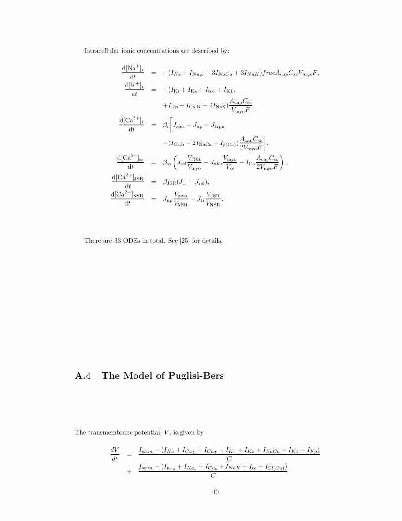
A.4 The Model of Puglisi-Bers

The transmembrane potential, V , is given by

dV

dt=

Istim − (INa + ICaL + ICaT + IKr + IKs + INaCa + IK1 + IKp)

C

+Istim − (IpCa + INab + ICab + INaK + Ito + ICl(Ca))

C

40

There are nine gating equations:

dm

dt= αm(1−m)− βmm,

dh

dt= αh(1− h)− βhh,

dj

dt= αj(1− j)− βjj,

dd

dt= αd(1− d)− βdd,

df

dt= αf (1− f)− βff,

db

dt=

b∞ − bτb

,

dg

dt=

g∞ − gτg

,

dXr

dt=

Xr∞ −Xr

τXr,

dXs

dt=

Xs∞ −Xs

τXs

There are seven equations to describe ionic concentrations:

dNaidt

= −(INa + ICaNa + INab + 3INaCa + 3INaK)AcapVmyoF

,

dCaidt

= ((ICaCa + IpCa + ICab + ICaT )− INaCa)Acap

2VmyoF+ Irel

VJSRVmyo

+ (Ileak − Iup)VNSRVmyo

,

dKi

dt= −(ICaK + IKr + IKs + IK1 + IKp + Ito − 2INaK)

AcapVmyoF

,

dKo

dt= (ICaK + IKr + IKs + IK1 + IKp + Ito − 2INaK)

AcapVcleftF

,

dCaJSRdt

= −(Irel − ItrVNSRVJSR

),

dCaNSRdt

= −(((Ileak + Itr)− Iup)),dCafootdt

= (ICaCa)Acap

2VmyoFRAV

There are 17 ODEs in total. See [20] and the references within for more details. Also, see [1]

for a concise description of the model.

41