implications of discontinuous idf equations in generation ... · rbrh, porto alegre, v. 22, e52,...

Revista Brasileira de Recursos HídricosBrazilian Journal of Water ResourcesVersão On-line ISSN 2318-0331RBRH, Porto Alegre, v. 22, e52, 2017Scientific/Technical Article

http://dx.doi.org/10.1590/2318-0331.0217170004

This is an Open Access article distributed under the terms of the Creative Commons Attribution License, which permits unrestricted use, distribution, and reproduction in any medium, provided the original work is properly cited.

Implications of discontinuous IDF equations in generation of runoff hydrographs. Case study: IDF-Porto Alegre (8º DISME)

Implicações da utilização de equações IDF descontínuas na geração de hidrogramas de escoamento superficial. Estudo de caso: IDF-Porto Alegre (8º DISME)

Ana Luiza Helfer1, Fernando Dornelles1 and Joel Avruch Goldenfum1

1Universidade Federal do Rio Grande do Sul, Porto Alegre, RS, BrazilE-mails: [email protected] (ALH), [email protected] (FD), [email protected] (JAG)

Received: January 05, 2017 - Revised: May 09, 2017 - Accepted: July 12, 2017

ABSTRACT

The intensity-duration-frequency (IDF) equations establish the relationship between the intensity and the duration of an extreme precipitation associated to the probability of its occurrence. Some studies have fitted multiple IDF equations per rain gauge, valid for certain rain duration ranges. An example is the IDF equation for the 8th District of Meteorology of Porto Alegre rain gauge, established and published by the CPRM in the Pluviometric Atlas Project. The main objective of the present study is to evaluate the implication of using this type of IDF equation, referred to as a “discontinuous IDF equation”, in the generation of runoff hydrographs, using the mentioned IDF as case study. The methodology consisted in comparing the peak flow and the runoff volume of hydrographs generated by the discontinuous IDF equation with the hydrographs obtained by using a single IDF equation. The runoff hydrographs were generated for hypothetical basins with the following characteristics: contribution areas of 5, 20 and 80 km2; CN of 70, 80 and 90; and time of concentration of 20, 40, 60, 100 and 200 minutes. A 24-hour rainfall event was considered with return period of 5, 10, 25, 50 and 100 years. As results, it was observed that, in the case studied, the multiple IDF equation present a better fit to the observed rainfall data than the single IDF equation. However, the discontinuity at the transition point between the equations, depending on its magnitude, may present some influence on the peak flow and on the runoff volume due to occurrence of secondary peaks on the runoff hydrographs. Therefore, it is recommended that a maximum limit of discontinuity must be observed between the multiple equations in order to avoid the occurrence of secondary peaks in the runoff hydrographs.

Keywords: IDF; Hyetograph; Runoff hydrograph.

RESUMO

As equações ou curvas intensidade, duração e frequência (IDF) estabelecem a relação entre a intensidade e a duração de uma precipitação extrema associada à sua probabilidade de ocorrência. A maioria dos ajustes destas curvas é realizado por meio de apenas uma equação; no entanto alguns autores estabelecem curvas IDF múltiplas, com duas ou mais equações distintas, válidas para determinadas faixas de duração de chuva. É o caso, por exemplo da IDF do 8º Distrito de Meteorologia de Porto Alegre, estabelecida pela CPRM no âmbito do Projeto Atlas Pluviométrico. O presente trabalho teve como objetivo avaliar a implicação da utilização desta IDF, chamada, neste trabalho, equação IDF descontínua, na geração de hidrogramas de escoamento superficial, utilizando-se como estudo de caso a IDF mencionada. A metodologia consistiu em comparar a vazão de pico e o volume dos hidrogramas de escoamento gerados a partir da IDF descontínua com hidrogramas obtidos a partir de uma IDF de equação única. Os hidrogramas foram gerados para bacias hipotéticas com áreas de 5, 20 e 80 km2, para cada qual variou-se o parâmetro CN em 70, 80 e 90 e o tempo de concentração em 20, 40, 60, 100 e 200 minutos. Considerou-se um evento de chuva de 24 horas de duração com tempos de retorno de 5, 10, 25, 50 e 100 anos. Como resultado observou-se que, as equações IDF múltiplas apresentam melhor ajuste aos dados de precipitação observados do que a equação IDF única. No entanto, a magnitude da descontinuidade no ponto de transição entre as equações pode provocar alterações nos valores de vazão de pico e volume dos hidrogramas de escoamento devido ao surgimento de picos secundários. Dessa forma, recomenda-se que, quando forem ajustadas equações IDF múltiplas, se observe um limite máximo de descontinuidade entre as equações, de forma a evitar o surgimento de picos secundários nos hidrogramas de escoamento.

Palavras-chave: IDF; Hietograma; Hidrograma de escoamento superficial.

RBRH, Porto Alegre, v. 22, e52, 2017


INTRODUCTION

The intensity-duration-frequency (IDF) equations establish the relationship between the intensity and the duration of a rainfall event associated to the probability of its occurrence. IDF equations are often used in hydrological studies with rainfall-runoff models to determine peak flows and runoff volumes. The peak flows and runoff volumes are then used to dimension hydraulic structures, such as: conduits, spillways, manholes, loopholes, detention basins, infiltration trenches, channels, etc. (Tucci, 1993).

The pioneering work in the determination of IDF equations in Brazil was that of Pfafstetter (1957). However, this type of work, based on historical data series, needs updating over time. Therefore, it is possible to find several studies with updated IDF equations, such as Fendrich (1998), Silva (2009), Back et al. (2011), as well as hydrology textbooks, such as Collischonn and Dornelles (2013) and Tucci (1993) and in Municipal Urban Drainage Plans.

Most IDF equations are fitted by only one equation. However, some authors are defining IDFs with two or more distinct equations per rain gauge, valid for certain rain duration ranges. An example is the IDF equation of the 8th District of Meteorology (DISME) rain gauge in Porto Alegre, Brazil. The IDF equation was defined and published by the Serviço Geológico do Brasil (CPRM, 2015), in the Pluviometric Atlas Project. This Project is an action within the Geodiversity Surveys Program, whose purpose is to gather, consolidate and organize rainfall data collected in the national meteorological network (CPRM, 2015).

The use of multiple equations is intended to improve the line of best fit between the estimated and the observed data, but it causes a discontinuity at the transition point between the equations. This study aims to evaluate the implication of using this type of IDF equation (referred to as a discontinuous IDF equation) in surface runoff hydrographs, using the 8th DISME IDF equation established by the CPRM (2015) as case study.

CASE STUDY: 8TH DISME DISCONTINUOUS IDF EQUATION (CPRM, 2015)

The 8th DISME meteorological station (WMO code 83967) is located at the coordinates 30° 03’ 13” S and 51° 10’ 24” W and has been collecting continuous data since September 1974.

There are several IDF equations fitted to the observed rainfall data from this meteorological station. The studies include: Goldenfum, Camaño and Silvestrini (1991), Silveira (1996), Bemfica, Goldenfum and Silveira (2000) and CPRM (2015).

The following presents a brief description of the methodology adopted by the CPRM when defining the 8th DISME IDF equation. The complete methodology is presented in CPRM (2013). The specifically methodology regarding the 8th DISME IDF equation is presented in CPRM (2015).

The 8th DISME IDF equation was derived from annual maximum rainfall series obtained from the observed data for the Xperiod 1974-2014 and for the following rainfall duration: 5, 10, 15, 30 and 45 minutes; 1, 2, 3, 4, 8, 14, 20 and 24 hours. The annual maximum series were submitted to consistency tests in order to identify outliers. The following was also analyzed: i) the independence of the series applying the non-parametric test proposed by Wald and Wolfowitz (1943) for the level of significance

of 2% to 5%; ii) the homogeneity of the series by applying the non-parametric test proposed by Mann and Whitney (1947) for the significance level of 2% to 5%; and iii) the stationarity of the series, applying Spearman’s non-parametric test to the significance level of 2% to 5%. The annual maximum rainfall series for the rainfall durations mentioned above are available in CPRM (2015).

Once this was done, an empirical distribution was fitted to the values using the Weibull plotting formula. In sequence, the following theoretical distributions functions were tested: Generalized Pareto distribution, Generalized Extreme Value (GEV) distribution, Generalized Logistics distribution, Gamma distribution, Gumbel distribution and Exponential distribution. The parameters of the theoretical distributions were calculated by using the L-moments method (GREENWOOD et al., 1979; HOSKING, 1986, 1990). The goodness of fit test was then realized by comparing the theoretical and empirical distribution, using Kolmogorov–Smirnov (K-S) test, Chi-Squared test and Anderson-Darling test. The Exponential distribution was the one that best fitted the annual maximum rainfall series of the 8th DISME meteorological station.

The equation adopted to represent the family of curves obtained from the Exponential distribution was of the following type:

( )

b

daTi

t c=

+ (1)

where i is the rainfall intensity (mm/h), T is the return period (years), t is the rainfall duration (minutes), a, b, c and d are parameters of the equation.

The IDF equation parameters were then estimated using the generalized reduced gradient algorithm (GRG) developed by Lasdon and Waren (1981) to solve nonlinear problems. The optimization between the observed data and the calculated values was performed by minimizing the Root Mean Square Error (RMSE) (Equation 2) and the Mean Absolute Percent Error (MAPE) (Equation 3).

( )N 2

i ii 1

1RMSE xo xcN =

= −∑ (2)

N i i

i 1 i

xo xc1MAPEN xc=

−= ∑ (3)

where: ixo is the observed data at time i, ixc is the value calculated at time i and N is the total number of data points.

A maximum MAPE of 10% between the observed data and the values calculated with the equation was assumed as a premise for the definition of the IDF parameters for any rainfall duration and return period. The IDF parameters are presented in Table 1. These IDF parameters are valid for return periods of up to 100 years and for rainfall duration from 5 minutes to 24 hours. The IDF curves are presented in Figure 1.

Table 1. Parameters of the 8th DISME IDF equation (CPRM, 2015).Duration a b c d

5 ≤ t < 120 min 4,247.90 0.2097 25.20 1.1199120 ≤ t ≤ 1440 min 573.10 0.1889 0 0.7256


Helfer et al.

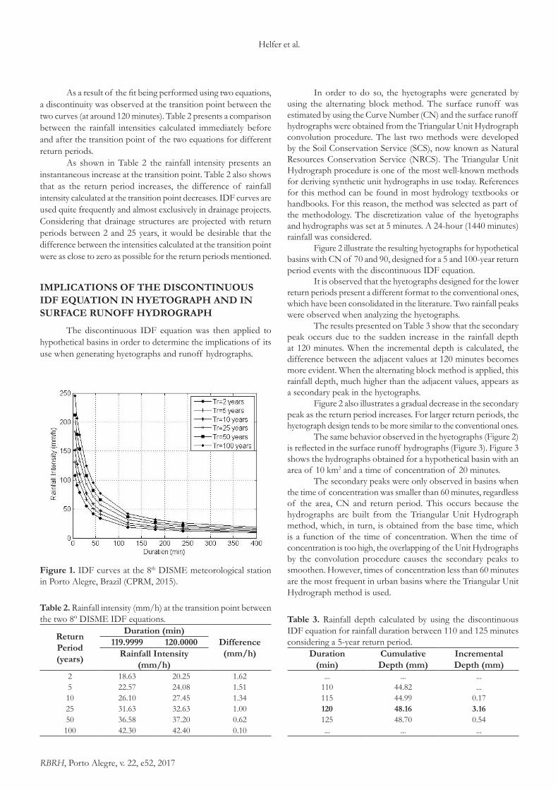
As a result of the fit being performed using two equations, a discontinuity was observed at the transition point between the two curves (at around 120 minutes). Table 2 presents a comparison between the rainfall intensities calculated immediately before and after the transition point of the two equations for different return periods.

As shown in Table 2 the rainfall intensity presents an instantaneous increase at the transition point. Table 2 also shows that as the return period increases, the difference of rainfall intensity calculated at the transition point decreases. IDF curves are used quite frequently and almost exclusively in drainage projects. Considering that drainage structures are projected with return periods between 2 and 25 years, it would be desirable that the difference between the intensities calculated at the transition point were as close to zero as possible for the return periods mentioned.

IMPLICATIONS OF THE DISCONTINUOUS IDF EQUATION IN HYETOGRAPH AND IN SURFACE RUNOFF HYDROGRAPH

The discontinuous IDF equation was then applied to hypothetical basins in order to determine the implications of its use when generating hyetographs and runoff hydrographs.

In order to do so, the hyetographs were generated by using the alternating block method. The surface runoff was estimated by using the Curve Number (CN) and the surface runoff hydrographs were obtained from the Triangular Unit Hydrograph convolution procedure. The last two methods were developed by the Soil Conservation Service (SCS), now known as Natural Resources Conservation Service (NRCS). The Triangular Unit Hydrograph procedure is one of the most well-known methods for deriving synthetic unit hydrographs in use today. References for this method can be found in most hydrology textbooks or handbooks. For this reason, the method was selected as part of the methodology. The discretization value of the hyetographs and hydrographs was set at 5 minutes. A 24-hour (1440 minutes) rainfall was considered.

Figure 2 illustrate the resulting hyetographs for hypothetical basins with CN of 70 and 90, designed for a 5 and 100-year return period events with the discontinuous IDF equation.

It is observed that the hyetographs designed for the lower return periods present a different format to the conventional ones, which have been consolidated in the literature. Two rainfall peaks were observed when analyzing the hyetographs.

The results presented on Table 3 show that the secondary peak occurs due to the sudden increase in the rainfall depth at 120 minutes. When the incremental depth is calculated, the difference between the adjacent values at 120 minutes becomes more evident. When the alternating block method is applied, this rainfall depth, much higher than the adjacent values, appears as a secondary peak in the hyetographs.

Figure 2 also illustrates a gradual decrease in the secondary peak as the return period increases. For larger return periods, the hyetograph design tends to be more similar to the conventional ones.

The same behavior observed in the hyetographs (Figure 2) is reflected in the surface runoff hydrographs (Figure 3). Figure 3 shows the hydrographs obtained for a hypothetical basin with an area of 10 km2 and a time of concentration of 20 minutes.

The secondary peaks were only observed in basins when the time of concentration was smaller than 60 minutes, regardless of the area, CN and return period. This occurs because the hydrographs are built from the Triangular Unit Hydrograph method, which, in turn, is obtained from the base time, which is a function of the time of concentration. When the time of concentration is too high, the overlapping of the Unit Hydrographs by the convolution procedure causes the secondary peaks to smoothen. However, times of concentration less than 60 minutes are the most frequent in urban basins where the Triangular Unit Hydrograph method is used.

Table 2. Rainfall intensity (mm/h) at the transition point between the two 8º DISME IDF equations.

Return Period (years)

Duration (min)Difference (mm/h)

119.9999 120.0000Rainfall Intensity

(mm/h)2 18.63 20.25 1.625 22.57 24.08 1.5110 26.10 27.45 1.3425 31.63 32.63 1.0050 36.58 37.20 0.62100 42.30 42.40 0.10

Figure 1. IDF curves at the 8th DISME meteorological station in Porto Alegre, Brazil (CPRM, 2015).

Table 3. Rainfall depth calculated by using the discontinuous IDF equation for rainfall duration between 110 and 125 minutes considering a 5-year return period.

Duration(min)

Cumulative Depth (mm)

Incremental Depth (mm)

... ... ...110 44.82 ...115 44.99 0.17120 48.16 3.16125 48.70 0.54... ... ...



Figure 2. Total rainfall (dotted line) and effective rainfall (solid line) calculated by the alternating block method using the discontinuous IDF equation, considering various CN and return period.

Figure 3. Surface runoff hydrographs obtained from the discontinuous IDF equation for a hypothetical basin with an area of 10 km2 and time of concentration of 20 minutes, considering various CN and return period.


Helfer et al.

According to Tucci (1993), a surface runoff hydrograph can be characterized by three main parts: ascension, highly correlated with the rainfall intensity; peak flow region, near the maximum value when the hydrograph begins to change its inflection as a result of the reduction of the rainfall and/or the basin attenuation; and depletion, when the flow or the water ponding begins to decrease on the surface. There is no mention of secondary or adjacent peaks in Tucci (1993) such as the hydrographs present in Figure 3 obtained from the discontinuous IDF equation.

The hydrographs main function is to allow the identification of the peak flow and the surface runoff volume, which in turn, are used to design hydraulic structures. Therefore, it is desirable that the hydrographs suitably represent the hydrological conditions during the hydraulic structure lifespan.

It is possible that the CPRM (2015) chose to use two equations to represent the IDF curves because this provides a better fit to the observed data. Besides that, by using two equations, the premise of obtaining a maximum Mean Absolute Percent Error (MAPE) of 10% between the calculated and the observed data was satisfied. However, as already shown, the surface runoff hydrographs obtained from two IDF equations presented secondary peaks when using the Triangular Unit Hydrograph method. These secondary peaks may possible affect the peak flow and the runoff volume value.

SINGLE IDF EQUATION

In order to evaluate the effects of the secondary peaks on the peak flow and on the runoff volume, a single IDF equation was fitted to the 8th DISME meteorological station data using the same methodology adopted by the CPRM (2015) in order to enable further comparison.

The Exponential distribution was fitted to the annual maximum rainfall series observed at the 8th DISME meteorological station for the following rainfall duration: 5, 10, 15, 30 and 45 minutes; 1, 2, 3, 4, 8, 14, 20 and 24 hours. The parameters of the Exponential distributions were calculated by using the L-moments method (GREENWOOD et al., 1979; HOSKING, 1986, 1990). The IDF equation parameters were then estimated using the generalized reduced gradient algorithm (GRG) developed by Lasdon and Waren (1981) to solve nonlinear problems. The optimization between the observed data and the calculated values was performed by minimizing the Root Mean Square Error (RMSE) and the Mean Absolute Percent Error (MAPE). The RMSE resulted in 4.55 mm/h and the MAPE in 5.65%.

The following IDF equation represents the best fit of a single IDF equation for the 8th DISME meteorological station, according to the methodology presented above, The IDF curves are presented in Figure 4.

( )

0,204

0,778787,388 Tit 8, 461

=+

(4)

where i is the rainfall intensity (mm/h), T is the return period (years) and t is the rainfall duration (minutes).

Table 4 present the relative difference between the rainfall intensities calculated by the single IDF equation and the rainfall

intensity observed at the 8th DISME meteorological station. Table 5 present the relative difference between the rainfall intensities calculated by the discontinuous IDF equation and the rainfall intensity observed at the 8th DISME station.

As expected, none of the IDFs reproduce exactly the observed data. However, the relative differences between the rainfall intensity calculated using the discontinuous IDF equation and the intensity observed are smaller than those calculated using the single IDF equation, for most return period and rainfall duration. On the other hand, when analyzing the absolute values (Table 6 and Table 7) the two fitted equations presents a maximum absolute difference of around 17 mm/h when compared to the observed data uncertainty which according to WMO (1994) is between 3 and 7%.

Table 4 also shows that the maximum relative differences between the observed data and the values calculated using the single IDF equation were higher than 10% at the cases highlighted in bold. In other words, the premise of having a relative difference less than 10% established by the CPRM (2015) was not satisfied when a single IDF equation was fitted.

COMPARISONS BETWEEN THE RUNOFF HYDROGRAPHS OBTAINED FROM THE SINGLE IDF EQUATION AND THOSE ONTAINED FROM THE DISCOUNTING IDF EQUATION

The comparison between the surface runoff hydrographs developed using the single IDF equation with those obtained using the discontinuous IDF equation was realized by comparing the peak flow and the runoff volume of both hydrographs according to the following equation:

( ) ( )( )

value single IDF value discontinuous IDF

value discontinuous IDF−

∆= (5)

Figure 4. IDF curves at the 8th DISME meteorological station fitted by a single equation.



Table 5. Relative difference between the rainfall intensity calculated using the discontinuous IDF equation and the rainfall intensity observed at the 8th DISME station, for several return periods and rainfall duration.

Rel

ativ

e D

iffer

ene

(%)

T (years)

Duration (min)5 10 15 30 45 60 120 180 240 480 840 1440

2 -4.1% 8.3% 10.0% 7.0% 5.1% 5.2% 6.0% 6.6% 6.6% 2.8% 0.5% 1.9%5 -9.3% -0.1% 1.4% -2.2% -4.6% -5.5% -2.7% 0.9% 1.3% -0.3% -5.0% -4.7%10 -10.1% -2.2% -0.7% -4.7% -7.2% -8.6% -5.4% -0.3% 0.2% -0.2% -6.2% -6.5%15 -9.7% -2.3% -0.8% -4.9% -7.6% -9.2% -6.0% -0.2% 0.4% 0.5% -6.1% -6.7%20 -9.0% -1.9% -0.4% -4.7% -7.5% -9.2% -6.0% 0.2% 0.9% 1.4% -5.7% -6.5%25 -8.3% -1.4% 0.1% -4.3% -7.1% -9.0% -5.9% 0.7% 1.4% 2.1% -5.3% -6.1%50 -5.4% 1.1% 2.7% -2.1% -5.1% -7.2% -4.5% 3.1% 3.9% 5.3% -3.1% -4.3%75 -3.0% 3.2% 4.9% -0.1% -3.3% -5.5% -3.1% 5.1% 5.9% 7.7% -1.3% -2.6%100 -1.1% 5.0% 6.7% 1.6% -1.7% -4.1% -1.9% 6.7% 7.6% 9.6% 0.2% -1.3%

Table 6. Absolute difference between the rainfall intensity (mm/h) calculated using the single IDF equation and the rainfall intensity observed at the 8th DISME station, for several return periods and rainfall duration.

Abs

olut

e D

iffer

ence

(mm

/h)

T (years)

Duration (min)5 10 15 30 45 60 120 180 240 480 840 1440

2 7.1 9.7 6.4 1.5 1.0 1.6 1.6 1.2 0.9 0.1 0.1 0.15 0.0 2.5 0.0 4.4 4.0 2.7 0.2 0.7 0.6 0.0 0.4 0.410 2.1 0.3 2.7 7.4 6.6 5.0 0.3 0.8 0.6 0.1 0.5 0.515 1.8 0.8 3.3 8.5 7.6 5.9 0.3 1.1 0.8 0.3 0.5 0.520 0.8 0.5 3.3 8.9 8.1 6.3 0.2 1.3 1.1 0.4 0.5 0.525 0.4 0.0 2.9 9.0 8.3 6.6 0.0 1.6 1.3 0.6 0.4 0.550 6.8 3.9 0.1 8.3 8.0 6.5 1.0 2.8 2.2 1.2 0.2 0.375 12.7 7.8 2.9 6.9 7.1 5.8 1.9 3.7 3.0 1.7 0.1 0.2100 17.9 11.3 5.7 5.4 6.1 5.1 2.8 4.5 3.7 2.1 0.3 0.1

Table 7. Absolute difference between the rainfall intensity (mm/h) calculated using the discontinuous IDF equation and the rainfall intensity observed at the 8th DISME station, for several return periods and rainfall duration.

Abs

olut

e D

iffer

ence

(mm

/h) T

(years)Duration (min)

5 10 15 30 45 60 120 180 240 480 840 14402 4.6 7.0 7.1 3.6 2.0 1.7 1.1 0.9 0.8 0.2 0.0 0.15 13.5 0.1 1.3 1.5 2.4 2.4 0.7 0.2 0.2 0.0 0.3 0.210 17.0 2.9 0.8 3.8 4.6 4.5 1.6 0.1 0.0 0.0 0.4 0.315 17.6 3.2 0.9 4.4 5.3 5.2 1.9 0.0 0.1 0.1 0.5 0.420 17.4 2.9 0.5 4.4 5.5 5.5 2.0 0.1 0.2 0.2 0.5 0.425 16.7 2.3 0.1 4.2 5.5 5.7 2.0 0.2 0.3 0.2 0.4 0.450 12.0 1.9 4.0 2.3 4.4 5.2 1.7 0.8 0.9 0.7 0.3 0.375 7.2 6.1 7.8 0.1 3.0 4.2 1.3 1.4 1.4 1.1 0.1 0.2100 2.8 9.9 11.2 1.9 1.6 3.3 0.8 2.0 1.8 1.4 0.0 0.1

Table 4. Relative difference between the rainfall intensity calculated using the single IDF equation and the rainfall intensity observed at the 8th DISME station, for several return periods and rainfall duration.

Rel

ativ

e D

iffer

ence

(%)

T (years)

Duration (min)5 10 15 30 45 60 120 180 240 480 840 1440

2 6.3% 11.5% 9.0% 2.9% 2.4% 5.1% 8.3% 8.5% 7.8% 1.6% -3.0% -4.1%5 0.0% 2.3% 0.0% -6.4% -7.5% -6.1% 0.8% 4.2% 3.9% 0.0% -7.0% -9.1%10 -1.2% -0.2% -2.4% -9.1% -10.4% -9.6% -0.9% 4.0% 3.8% 1.1% -7.2% -9.9%15 -1.0% -0.5% -2.7% -9.6% -11.0% -10.4% -0.9% 4.8% 4.7% 2.4% -6.6% -9.5%20 -0.4% -0.4% -2.6% -9.5% -11.0% -10.5% -0.5% 5.7% 5.7% 3.7% -5.8% -8.9%25 0.2% 0.0% -2.2% -9.2% -10.8% -10.4% 0.0% 6.6% 6.6% 4.9% -5.0% -8.2%50 3.0% 2.2% -0.1% -7.5% -9.2% -9.0% 2.5% 10.2% 10.4% 9.3% -1.8% -5.4%75 5.3% 4.1% 1.8% -5.8% -7.6% -7.6% 4.7% 13.0% 13.2% 12.5% 0.7% -3.2%100 7.2% 5.8% 3.4% -4.4% -6.3% -6.3% 6.4% 15.2% 15.5% 15.0% 2.7% -1.4%


Helfer et al.

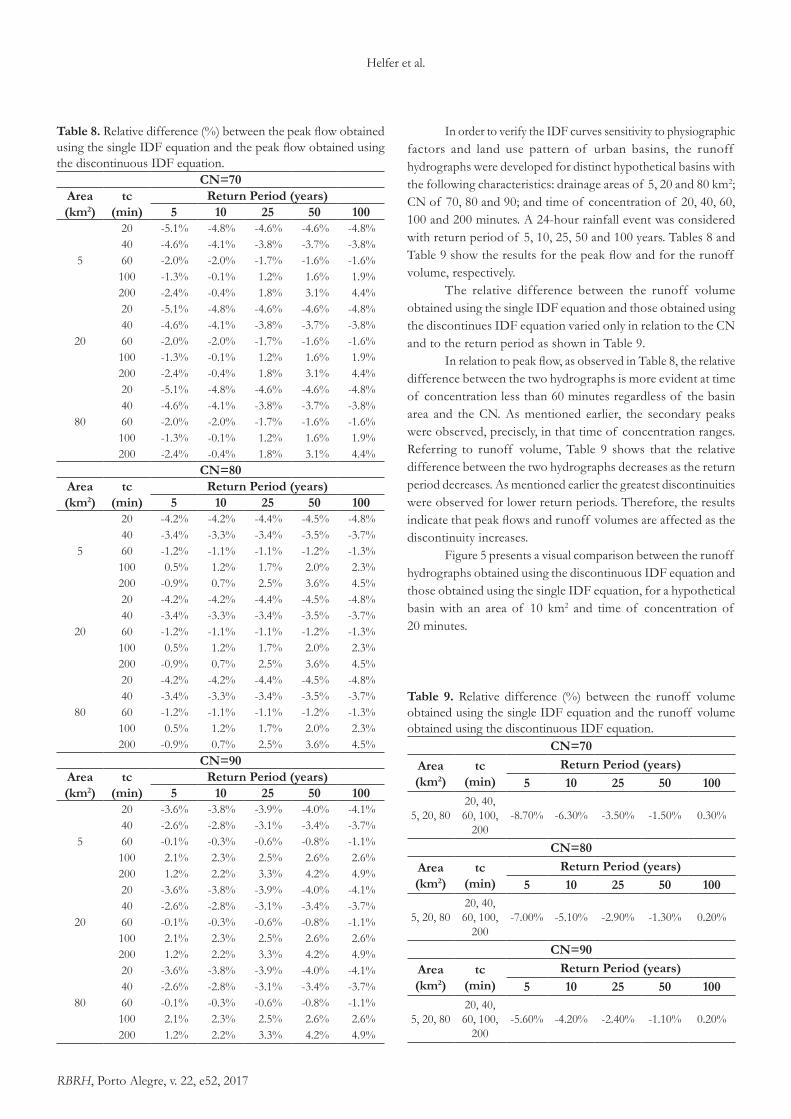
Table 8. Relative difference (%) between the peak flow obtained using the single IDF equation and the peak flow obtained using the discontinuous IDF equation.

CN=70Area (km2)

tc (min)

Return Period (years)5 10 25 50 100

5

20 -5.1% -4.8% -4.6% -4.6% -4.8%40 -4.6% -4.1% -3.8% -3.7% -3.8%60 -2.0% -2.0% -1.7% -1.6% -1.6%100 -1.3% -0.1% 1.2% 1.6% 1.9%200 -2.4% -0.4% 1.8% 3.1% 4.4%

20

20 -5.1% -4.8% -4.6% -4.6% -4.8%40 -4.6% -4.1% -3.8% -3.7% -3.8%60 -2.0% -2.0% -1.7% -1.6% -1.6%100 -1.3% -0.1% 1.2% 1.6% 1.9%200 -2.4% -0.4% 1.8% 3.1% 4.4%

80

20 -5.1% -4.8% -4.6% -4.6% -4.8%40 -4.6% -4.1% -3.8% -3.7% -3.8%60 -2.0% -2.0% -1.7% -1.6% -1.6%100 -1.3% -0.1% 1.2% 1.6% 1.9%200 -2.4% -0.4% 1.8% 3.1% 4.4%

CN=80Area (km2)

tc (min)


5

20 -4.2% -4.2% -4.4% -4.5% -4.8%40 -3.4% -3.3% -3.4% -3.5% -3.7%60 -1.2% -1.1% -1.1% -1.2% -1.3%100 0.5% 1.2% 1.7% 2.0% 2.3%200 -0.9% 0.7% 2.5% 3.6% 4.5%

20

20 -4.2% -4.2% -4.4% -4.5% -4.8%40 -3.4% -3.3% -3.4% -3.5% -3.7%60 -1.2% -1.1% -1.1% -1.2% -1.3%100 0.5% 1.2% 1.7% 2.0% 2.3%200 -0.9% 0.7% 2.5% 3.6% 4.5%

80

20 -4.2% -4.2% -4.4% -4.5% -4.8%40 -3.4% -3.3% -3.4% -3.5% -3.7%60 -1.2% -1.1% -1.1% -1.2% -1.3%100 0.5% 1.2% 1.7% 2.0% 2.3%200 -0.9% 0.7% 2.5% 3.6% 4.5%

CN=90Area (km2)

tc (min)


5

20 -3.6% -3.8% -3.9% -4.0% -4.1%40 -2.6% -2.8% -3.1% -3.4% -3.7%60 -0.1% -0.3% -0.6% -0.8% -1.1%100 2.1% 2.3% 2.5% 2.6% 2.6%200 1.2% 2.2% 3.3% 4.2% 4.9%

20

20 -3.6% -3.8% -3.9% -4.0% -4.1%40 -2.6% -2.8% -3.1% -3.4% -3.7%60 -0.1% -0.3% -0.6% -0.8% -1.1%100 2.1% 2.3% 2.5% 2.6% 2.6%200 1.2% 2.2% 3.3% 4.2% 4.9%

80

20 -3.6% -3.8% -3.9% -4.0% -4.1%40 -2.6% -2.8% -3.1% -3.4% -3.7%60 -0.1% -0.3% -0.6% -0.8% -1.1%100 2.1% 2.3% 2.5% 2.6% 2.6%200 1.2% 2.2% 3.3% 4.2% 4.9%

In order to verify the IDF curves sensitivity to physiographic factors and land use pattern of urban basins, the runoff hydrographs were developed for distinct hypothetical basins with the following characteristics: drainage areas of 5, 20 and 80 km2; CN of 70, 80 and 90; and time of concentration of 20, 40, 60, 100 and 200 minutes. A 24-hour rainfall event was considered with return period of 5, 10, 25, 50 and 100 years. Tables 8 and Table 9 show the results for the peak flow and for the runoff volume, respectively.

The relative difference between the runoff volume obtained using the single IDF equation and those obtained using the discontinues IDF equation varied only in relation to the CN and to the return period as shown in Table 9.

In relation to peak flow, as observed in Table 8, the relative difference between the two hydrographs is more evident at time of concentration less than 60 minutes regardless of the basin area and the CN. As mentioned earlier, the secondary peaks were observed, precisely, in that time of concentration ranges. Referring to runoff volume, Table 9 shows that the relative difference between the two hydrographs decreases as the return period decreases. As mentioned earlier the greatest discontinuities were observed for lower return periods. Therefore, the results indicate that peak flows and runoff volumes are affected as the discontinuity increases.

Figure 5 presents a visual comparison between the runoff hydrographs obtained using the discontinuous IDF equation and those obtained using the single IDF equation, for a hypothetical basin with an area of 10 km2 and time of concentration of 20 minutes.

Table 9. Relative difference (%) between the runoff volume obtained using the single IDF equation and the runoff volume obtained using the discontinuous IDF equation.

CN=70Area (km2)

tc (min)


5, 20, 8020, 40, 60, 100,

200-8.70% -6.30% -3.50% -1.50% 0.30%

CN=80Area (km2)

tc (min)


5, 20, 8020, 40, 60, 100,

200-7.00% -5.10% -2.90% -1.30% 0.20%

CN=90Area (km2)

tc (min)


5, 20, 8020, 40, 60, 100,

200-5.60% -4.20% -2.40% -1.10% 0.20%



Figure 5. Visual comparison between the runoff hydrographs obtained using the discontinuous IDF equation and those obtained using the single IDF equation for a hypothetical basin with an area of 10 km2 and time of concentration of 20 minutes.

CONCLUSIONS

The multiple IDF equation fit was compared to the single IDF equation fit. The comparison was motivated only by the discontinuity effect at the transition point between the multiple curves.

In the case studied, regarding to relative differences, the multiple IDF equation presented better fit to the observed rainfall data than the single IDF equation for most return period and rainfall duration analyzed. However, regarding to absolute differences, the maximum absolute difference between the rainfall intensities calculated and the rainfall intensities observed was around 17 mm/h for both equations.

The implications of the multiple IDF equation in runoff hydrographs was also analyzed. In the case studied, the discontinuity at the transition point between the equations (at around 120 minutes), depending on its magnitude, may present some influence on the peak flow and on the runoff volume due to occurrence of secondary peaks on the runoff hydrographs. As it could be observed, the greater the discontinuity between the equations, the greater its influence on the peak flow and on the runoff volume.

Therefore, it is recommended that a maximum limit of discontinuity between the multiple equations must be observed in order to avoid the occurrence of secondary peaks in the runoff hydrographs. The problem can be solved by including constraints on the curve fitting routine.

Further researches are suggested in order to determine a maximum admissible limit between the multiple equations.

ACKNOWLEDGEMENTS

The authors are grateful to CAPES for the master grant provided to the first author and to CNPq for promoting research and conferring a research productivity grant to the other authors. We also thank the anonymous reviewers for providing insightful comments that helped to improve the manuscript.

REFERENCES

BACK, A. J.; HENN, A.; OLIVEIRA, J. L. R. Heavy rainfall equations for Santa Catarina, Brazil. Revista Brasileira de Ciência do


Helfer et al.

Solo, v. 35, n. 6, p. 2127-2134, 2011. http://dx.doi.org/10.1590/S0100-06832011000600027.

BEMFICA, D. C.; GOLDENFUM, J. A.; SILVEIRA, A. L. L. Análise da aplicabilidade de padrões de chuva de projeto a Porto Alegre. Revista Brasileira de Recursos Hídricos., v. 5, n. 4, p. 5-16, 2000. http://dx.doi.org/10.21168/rbrh.v5n4.p5-16.

COLLISCHONN, W.; DORNELLES, F. Hidrologia para engenharia e ciências ambientais. 1. ed. Porto Alegre: ABRH, 2013. 336 p. v. 1.

FENDRICH, R. Chuvas intensas para obras de drenagem no Estado do Paraná. Curitiba: Champagnat, 1998. 99 p.

GOLDENFUM, J. A.; CAMAÑO, B.; SILVESTRINI, J. Análise das chuvas intensas em Porto Alegre. [S.l.]: [s.n.], 1991.

GREENWOOD, J. A.; LANDWEHR, J. M.; MATALAS, N. C.; WALLIS, J. R. Probability weighted moments: definition and relation to parameters of several distributions espressable in inverse form. Water Resources Research, v. 15, n. 5, p. 1049-1054, 1979. http://dx.doi.org/10.1029/WR015i005p01049.

HOSKING, J. R. M. The theory of probabilty weightes moments. New York: IBM Research Division, 1986. 160 p. IBM Research Report RC 12210.

HOSKING, J. R. M. L-moments: analysis and estimation of distributions usinglinear combinations of order statistics. Journal of the Royal Statistical Society. Series B. Methodological, v. 52, n. 2, p. 105-124, 1990.

LASDON, L. S.; WAREN, A. D. GRG2: an all FORTRAN general purpose nonlinear optimizer. ACM SIGMAP Bulletin, v. 30, n. 30, p. 10-11, 1981. http://dx.doi.org/10.1145/1111268.1111270.

MANN, H. B.; WHITNEY, D. R. On the test of whether one of two random variables is stochastically larger than the other. Annals of Mathematical Statistics, v. 18, n. 1, p. 50-60, 1947. http://dx.doi.org/10.1214/aoms/1177730491.

PFAFSTETTER, O. Chuvas intensas no Brasil: relação entre precipitação, duração e frequência de chuvas em 98 postos com pluviógrafos. Rio de Janeiro: DNOS, 1957. 419 p.

SERVIÇO GEOLÓGICO DO BRASIL – CPRM. Atlas pluviométrico do Brasil: metodologia para definição das equações intensidade-duração-frequência do projeto atlas pluviométrico. Belo Horizonte: CPRM, 2013. 48 p.

SERVIÇO GEOLÓGICO DO BRASIL – CPRM. Atlas Pluviométrico do Brasil: equações intensidade-duração-frequência. Município: Porto Alegre. Estação Pluviográfica: Porto Alegre, Códigos 03051011 (ANA) e 83967 (OMM). Porto Alegre: CPRM, 2015. 14 p.

SILVA, B. M. Chuvas intensas em localidades do Estado de Pernambuco. 2009. 116 f. Dissertação (Mestrado) - Universidade Federal de Pernambuco, Recife, 2009.

SILVEIRA, A. L. L. Contribution à i’etude hydrologique d’un bassin semi-urbanisé dans le Brésil subtropical: bassin de i’arroio dilúvio à Porto Alegre. 1996. 242 f. Thése (Docrorat). Université Montpellier II, 1996.

TUCCI, C. E. M. (Ed.). Hidrologia: ciência e aplicação. 4. ed. Porto Alegre: Editora da Universidade, ABRH, 1993. 943 p. (Coleção ABRH).

WALD, A.; WOLFOWITZ, J. An exact test for randomness in the non-parametric case based on serial correlation. Annals of Mathematical Statistics, v. 14, n. 4, p. 378-388, 1943. http://dx.doi.org/10.1214/aoms/1177731358.

WORLD METEOROLOGICAL ORGANIZATION – WMO. Guide to hydrological practices: data acquisition and processing, analysis, forecasting and other applications. Geneva, 1994. n. 168.

Authors contributions

Ana Luiza Helfer: Performed the methodology, obtained the results and wrote the text.

Fernando Dornelles: Defined the objectives, purposes and revised the text.

Joel Avruch Goldenfum: Contributed with technical discussions and revised the text.

http://dx.doi.org/10.1590/S0100-06832011000600027

http://dx.doi.org/10.1590/S0100-06832011000600027

http://dx.doi.org/10.21168/rbrh.v5n4.p5-16

http://dx.doi.org/10.1029/WR015i005p01049

http://dx.doi.org/10.1145/1111268.1111270

http://dx.doi.org/10.1214/aoms/1177730491




implications of discontinuous idf equations in generation ... · rbrh, porto alegre, v. 22, e52,...

Documents