Ambiguity Aversion: Implications for the UncoveredInterest Rate Parity Puzzle∗

Cosmin L. Ilut†

First draft: October 2008This draft: March 2009

Abstract

Empirically, high-interest-rate currencies tend to appreciate in the future relativeto low-interest-rate currencies instead of depreciating as uncovered interest rate parity(UIP) states. The explanation for the UIP puzzle that I pursue in this paper isthat the agents’ beliefs are systematically distorted. This perspective receives somesupport from an extended empirical literature using survey data. I construct a modelof exchange rate determination in which ambiguity-averse agents need to solve afiltering problem to form forecasts but face signals about the time-varying hiddenstate that are of uncertain precision. In the presence of such uncertainty, ambiguity-averse agents take a worst-case evaluation of this precision and respond strongerto bad news than to good news about the payoffs of their investment strategies.Importantly, because of this endogenous systematic underestimation, agents in thenext periods will perceive on average positive innovations about the payoffs whichwill make them re-evaluate upwards the profitability of the strategy. As a result,the model’s dynamics imply significant ex-post departures from UIP as equilibriumoutcomes. In addition to providing a resolution to the UIP puzzle, the model predicts,consistent with the data, negative skewness and excess kurtosis for currency excessreturns and positive average payoffs even for hedged positions.

Key Words: uncovered interest rate parity, ambiguity aversion, robust filtering.JEL Classification: D8, E4, F3, G1.

∗I am grateful to the members of my dissertation committee Lawrence Christiano, Martin Eichenbaum,Giorgio Primiceri and Sergio Rebelo for their continuous support and advice. I would also like to thankGadi Barlevy, Peter Benczur, Eddie Dekel, Lars Hansen, Nicolas Lehmann-Ziebarth, Ricardo Massolo,Jonathan Parker, Tom Sargent, Tomasz Strzalecki and seminar participants at the Board of Governors,Chicago Fed, Duke, ECB, New York Fed, NYU, Northwestern, Philadelphia Fed, UC Davis, UC SantaCruz and Univ. of Virginia for helpful discussions and comments.†Department of Economics, Northwestern University. E-mail: cosminilut2009@u.northwestern.edu

1 Introduction

According to uncovered interest rate parity (UIP), periods when the domestic interest

rate is higher than the foreign interest rate should on average be followed by periods of

domestic currency depreciation. An implication of UIP is that a regression of realized

exchange rate changes on interest rate differentials should produce a coefficient of 1.

This implication is strongly counterfactual. In practice, UIP regressions (Hansen and

Hodrick (1980), Fama (1984)) produce coefficient estimates well below 1 and sometimes

even negative.1 This anomaly is taken very seriously because the UIP equation is a property

of most open economy models. The failure, referred to as the UIP puzzle or the forward

premium puzzle2, implies that traders who borrow in low-interest-rate currencies and lend in

high-interest-rate currencies (a strategy known as the “carry trade”) make positive profits

on average. The standard approach in addressing the UIP puzzle has been to assume

rational expectations and time-varying risk premia. This approach has been criticized

in two ways: survey evidence has been used to cast doubt on the rational expectations

assumption3 and other empirical research challenges the risk implications of the analysis.4

In this paper, I follow a conjecture in the literature that the key to understanding

the UIP puzzle lies in departing from the rational expectations assumption.5 I pursue

this conjecture formally, using the assumption that agents are not endowed with complete

knowledge of the true data generating process (DGP) and that they confront this uncer-

tainty with ambiguity aversion. I model ambiguity aversion along the lines of the maxmin

expected utility (or multiple priors) preferences as in Gilboa and Schmeidler (1989).

The model has several types of agents. The decision problem of a subset of the agents (I

call them ‘agents’) is modeled explicitly, and the behavior of the others (‘liquidity traders’)

is taken as given. The supply of domestic and foreign bonds is fixed in domestic and foreign

currency units, respectively. The liquidity traders adjust their demand for bonds to satisfy

1Among recent studies see Chinn and Frankel (2002), Gourinchas and Tornell (2004), Chinn andMeredith (2005), Sarno (2005), Verdelhan (2006) and Burnside et al. (2008).

2Under covered interest rate parity the interest rate differential equals the forward discount. The UIPpuzzle can then be restated as the observation that currencies at a forward discount tend to appreciate.

3For example, Froot and Frankel (1989), Chinn and Frankel (2002) and Bacchetta et al. (2008) findthat most of the predictability of currency excess returns is due to expectational errors.

4See Lewis (1995) and Engel (1996) for surveys on this research. See Burnside et al. (2008) for a criticalreview of recent risk-based explanations. These criticisms are by no means definitive as there is a recentrisk-based theoretical literature, including for example Verdelhan (2006), Bansal and Shaliastovich (2007),Alvarez et al. (2008) and Farhi and Gabaix (2008) that argues that the typical empirical exercises areunable by construction to capture the underlying time-variation in risk.

5Froot and Thaler (1990), Eichenbaum and Evans (1995), Lyons (2001) and Gourinchas and Tornell(2004) argue that models where agents are slow to respond to news may explain the UIP puzzle.

1

the market clearing condition. Agents are all identical and live for two periods.6 The

representative agent begins the first period with no endowment. She buys and sells bonds

in different currencies in order to maximize a negative exponential utility function of second

period wealth. The only source of randomness in the environment is the domestic/foreign

interest rate differential. I model this as an exogenous stochastic process, which is the

sum of unobserved persistent and transitory components. As a result, the agent must

solve a signal extraction problem when she wants to adjust her forecasts in response to a

disturbance.

I follow and extend the setup in Epstein and Schneider (2007, 2008) by assuming that

the agent does not know the variances of the innovations in the temporary and persistent

components and she allows for the possibility that those variances change over time. In

other words, the agent perceives the signals she receives about the hidden persistent state

as having uncertain precision or quality. Under ambiguity aversion with maxmin expected

utility, the agent simultaneously chooses a belief about the model parameter values and a

decision about how many bonds to buy and sell. The bond decision maximizes expected

utility subject to the chosen belief and the budget constraint. The belief is chosen so

that, conditional on the agent’s bond decision, expected utility is minimized subject to

a particular constraint. The constraint is that the agent only considers an exogenously-

specified finite set of values for the variances. I choose this set so that, in equilibrium, the

variance parameters selected by the agent are not implausible in a likelihood ratio sense.

In equilibrium, the agent invests in the higher interest rate bond (investment currency)

by borrowing in the lower interest rate bond (funding currency). The higher the estimate of

the hidden state of the investment differential, i.e. the differential between the high-interest-

rate and the low-interest-rate, the larger her demand for this strategy is. Conditional on

this decision, the agent’s expected utility is decreasing in the expected future depreciation

of the investment currency. In equilibrium, this depreciation will be stronger when the

future demand for the investment currency is lower. Thus, the agent is concerned that the

observed investment differential in the future is low which makes the agent worry that the

estimate of the hidden state of the investment differential is low. As a result, the initial

concern for a depreciation translates into the agent tending to underestimate, compared to

the true DGP, the hidden state of this differential. When faced with signals of uncertain

precision, ambiguity-agents act cautiously and underestimate the hidden state by reacting

asymmetrically to news: they believe that it is more likely that observed increases in the

investment differential have been generated by temporary shocks (low precision of signals)

6The agents in my model resemble those in Bacchetta and van Wincoop (2008), except that there theyinvestigate rational inattention and I assume ambiguity aversion.

2

while decreases as reflecting more persistent shocks (high precision of signals). The UIP

condition holds ex-ante under these endogenously pessimistic beliefs.7

Because the agent underestimates, compared to the true DGP, the persistent component

of the investment differential she is on average surprised next period by observing a higher

investment differential than expected. Under her subjective beliefs these innovations are

unexpected good news that increase the estimate of the hidden state. This updating effect

creates the possibility that next period the agent finds it optimal to invest even more in

the investment currency because this higher estimate raises the present value of the future

payoffs of investing in the higher interest rate bond. The increased demand will drive up the

value of the investment currency contributing to a possible appreciation of the investment

currency. Thus, an investment currency could see a subsequent equilibrium appreciation

instead of a depreciation as UIP predicts.

The main result of this paper is that such a model of exchange rate determination has

the potential to resolve the UIP puzzle. Indeed, for the benchmark calibration, numerical

simulations show that in large samples the UIP regression coefficient is negative and

statistically significant while in small samples it is mostly negative and statistically not

different from zero. The model is calibrated to data for eight developed countries which

suggests a high degree of persistence of the hidden state and a relatively large signal to

noise ratio for the true DGP. In the benchmark specification I impose some restrictions

on the frequency and magnitudes of the distortions that the agent is considering so that

the equilibrium distorted sequence of variances is difficult to distinguish statistically from

the true DGP based on a likelihood comparison. Eliminating these constraints would

qualitatively maintain the same intuition and generate stronger quantitative results at the

expense of the agent seeming less interested in the statistical plausibility of her distorted

beliefs. Studying other parameterizations, I find that the UIP regression coefficient becomes

positive, even though smaller than 1, if the true DGP is characterized by a significantly less

persistent hidden state or much larger temporary shocks than the benchmark specification.

The gradual incorporation of good news implied by this model can directly account also

for the delayed overshooting puzzle. This is an empirically documented impulse response8

in which following a positive shock to the domestic interest rate the domestic currency

experiences a gradual appreciation for several periods instead of an immediate appreciation

and then a path of depreciation as UIP implies. For such an experiment, the ambiguity-

7In fact, the equilibrium condition is a risk-adjusted version of UIP which incorporates a risk-premium.However, as detailed in the model, this risk-correction is extremely small.

8See Eichenbaum and Evans (1995), Grilli and Roubini (1996), Faust and Rogers (2003) and Scholl andUhlig (2006).

3

averse agent invests in equilibrium in the domestic currency and thus is worried about its

future depreciation. The equilibrium beliefs then imply that the agent tends to overweigh,

compared to the true DGP, the possibility that the observed increase in the interest rate

reflects the temporary shock. This underestimation generates the gradual incorporation of

the initial shock into the estimate and the demand of the ambiguity-averse agent.

The intuition for the model’s ability to explain the UIP puzzle is related to Gourinchas

and Tornell (2004) who show that if, for some unspecified reason, the agent systematically

underreacts to signals about the time-varying hidden-state of the interest rate differential

this can address the UIP and the delayed overshooting puzzle. The main difference is

that here I investigate a model which addresses the origin and optimality of such beliefs.

This model generates endogenous underreaction only to good news, with the agent in fact

overreacting to bad news.

Related to the work presented here, Li and Tornell (2008) show that if the agent only

cares about the mean square error of the estimate of the hidden state and she is concerned

only about uncertainty in the observation equation then the robust Kalman gain is lower

than in the reference model, thus implying underreaction to news. As an alternative model

to generate an endogenous slow response to news, Bacchetta and van Wincoop (2008) use

ideas from the rational inattention literature. In their setup, since information is costly to

acquire and to process, some investors optimally choose to be inattentive and revise their

portfolios infrequently. Their model implies that agents respond symmetrically to news.

The explanation for the UIP puzzle proposed in this paper relies on placing structure

on the type of uncertainty that the agent is concerned about. The agent receives signals of

uncertain precision about a time-varying hidden state but otherwise she trusts the other

elements of her representation of the DGP. Because of the structured uncertainty, the

equilibrium distorted belief is not equivalent to the belief generated by simply increasing

the risk aversion and using the rational expectations assumption.9

Besides providing an explanation for the UIP puzzle, the theory for exchange rate

determination proposed in this paper has several implications for the carry trade. First,

directly related to the resolution of the UIP puzzle, the benchmark calibration produces, as

in the data, positive average payoffs for the carry trade strategy. Compared to the empirical

evidence, the model implied payoffs are smaller and less variable. The model generates

positive average payoffs because in equilibrium the subjective probability distribution differs

from the objective one by overpredicting bad events and underpredicting good events.

9This is in contrast to unstructured uncertainty, for which, as shown for example in Strzalecki (2007),Barillas et al. (2008), the multiplier preferences used in Hansen and Sargent (2008) are equivalent to ahigher risk aversion expected utility.

4

Second, in the model hedged positions can deliver positive mean payoffs. Empirically,

Burnside et al. (2008) and Jurek (2008) find significant evidence of this type of profitability.

The difficulty in generating this result is related to the intuition that buying insurance

against the downside risk produces on average negative payoffs that decrease the payoff of

the hedged strategy. My model also implies this type of loss because of the overprediction

of bad events. However, in the model this negative payoff does not completely offset the

positive payoff of the unhedged carry trade. The reason is related to the significantly

more frequent occurrence of good states for the carry trade strategy under the objective

probability distribution than under the equilibrium distorted beliefs. This is in contrast

to models in which peso events are associated with large losses for the unhedged carry

trade strategy that do not occur in the sample but otherwise, for the non-peso events,

the subjective and the probability distributions coincide.10 The theory presented in this

paper is also consistent with recent empirical findings documented in Jurek (2008) about

the conditional time-variation of risk-neutral moments for currency trading.

Third, the model implies that carry trade payoffs are characterized by negative skewness

and excess kurtosis. This is consistent with the data as recent evidence (Brunnermeier

et al. (2008)) suggests that high interest rate currencies tend to appreciate slowly but

depreciate suddenly. In my model, an increase in the high-interest-rate compared to the

market’s expectation produces, relatively to rational expectations, a slower appreciation

of the investment currency since agents underreact to this type of innovations. However,

a decrease in this rate generates a relatively sudden depreciation because agents respond

quickly to that type of news.11 The excess kurtosis is a manifestation of the diminished

reaction to good news. The asymmetric response to news is also consistent with the high

frequency reaction of exchange rates to fundamentals documented in Andersen et al. (2003).

The remainder of the paper is organized as follows. Section 2 describes and discusses

the model. Section 3 presents a rational expectations version of the model to be contrasted

to the ambiguity averse version studied in Section 4. Section 5 presents the model impli-

cations for exchange rate determination and discusses alternative specifications. Section

6 concludes. In the Appendix I provide details on some of the model’s equations and

statements.

10For such models see for example Engel and Hamilton (1989), Lewis (1989), Kaminsky (1993) and Evansand Lewis (1995). See Burnside et al. (2008) for a discussion on the possibility that peso events explainthe UIP puzzle given the profitability of the hedged carry trade.

11Brunnermeier et al. (2008) argue that the data suggests that the realized skewness is related to therapid unwinding of currency positions, a feature that is replicated by my model. They propose shocksto funding liquidity as a mechanism for this endogeneity. See Burnside (2008) for a comment on thispossibility.

5

2 Model

2.1 Basic Setup

The basic setup is a typical one good, two-country, dynamic general equilibrium model of

exchange rate determination. The focus is to keep the model as simple as possible while

retaining the key ingredients needed to highlight the role of ambiguity aversion and signal

extraction.

There are overlapping generations (OLG) of investors who each live 2 periods, derive

utility from end-of-life wealth and are born with zero endowment. There is one good for

which purchasing power parity holds pt = p∗t + st, where pt is the log of price level of the

good in the Home country and st the log of the nominal exchange rate defined as the price

of the Home currency per unit of foreign currency (FCU). Foreign country variables are

indicated with a star. There are one-period nominal bonds in both currencies issued by the

respective governments. Domestic and foreign bonds are in fixed supply in the domestic

and foreign currency respectively.

The Home and Foreign nominal interest rates are it and i∗t respectively. The driving

exogenous force is the process for the interest rate differential rt = it − i∗t . The true DGP

is the state-space model:

rt = H ′xt + σV vt (2.1)

xt = Fxt−1 + σUut

The shocks ut and vt are Gaussian white noises. Thus, at time t the observable differential

rt is the sum of a hidden unobservable persistent (xt) and a temporary component (vt). The

agent entertains that the true DGP lies in a set of models (i.e. probability distributions over

outcomes). The specific assumptions about the subjective beliefs of the agents regarding

this process are covered in the next section.

Investors born at time t have a CARA utility over end-of-life wealth, Wt+1, with a rate

of absolute risk-aversion of γ. Their maxmin expected utility at time t is:

Vt = maxbt

minP∈Λ

EPt [− exp(−γWt+1)|It] (2.2)

where It is the information available at time t and bt is the amount of foreign bonds invested.

Agents have a zero endowment and pursue a zero-cost investment strategy: borrowing in

one currency and lending in another. Since PPP holds, Foreign and Home investors face

the same real returns and therefore will choose the same portfolio.

6

The set Λ comprises the alternative subjective probability distribution available to the

agent. They decide which of the the distributions (models) in the set Λ to use in forming

their subjective beliefs about the future exchange rate. I postpone the discussion about

the optimization over these beliefs to the next sections, noting that the optimal choice for

bt is made under the subjective probability distribution P .

The amount bt is expressed in domestic currency (USD). To illustrate the investment

position suppose that bt is positive. That means that the agent has borrowed bt in the

domestic currency and obtains bt1St

FCU units, where St = est . This amount is then

invested in foreign bonds and generates bt1St

exp(i∗t ) of FCU units at time t + 1. At time

t+ 1 the agent has to repay the interest rate bearing borrowed amount of bt exp(it). Thus,

the agent has to exchange back the time t + 1 proceeds from FCU into USD and obtains

btSt+1

Stexp(i∗t ). The net end-of-life is then a function of the amount of bonds invested and

the excess return:

Wt+1 = bt[exp(st+1 − st + i∗t )− exp(it)]

To close the model I specify a Foreign bond market clearing condition similar to

Bacchetta and van Wincoop (2008). There is a fixed supply B of Foreign bonds in the

Foreign currency. In steady state the investor holds no assets since she has zero endowment.

The steady state amount of bonds is held every period by some unspecified traders. They

can be interpreted as liquidity traders that have a constant bond demand. The real supply

of Foreign bonds is Be−p∗t = Best where the Home price level is normalized at 1. I also

normalize the steady state log exchange rate to 0. Thus, the market clearing condition is:

bt = Best −B (2.3)

where B is the steady state amount of Foreign bonds. Following Bacchetta and van

Wincoop (2008) I also set B = 0.5, corresponding to a two-country setup with half of the

assets supplied domestically and the other half by the rest of the world. By log-linearizing

the RHS of (2.3) around steady state I get the market clearing condition12:

bt = .5st (2.4)

12Bacchetta and van Wincoop (2008) analyze an alternative model with constant relative risk aversionin which agents are born with an endowment of one good and decide what fraction of it to invest in theforeign bond. The same equilibrium conditions are obtained as in this model except that those conditionsare expressed in deviations from steady state.

7

2.2 Model uncertainty

The key departure from the standard framework of rational expectations is that I drop

the assumption that the shock processes are random variables with known probability

distributions. The agent will entertain various possibilities for the data generating process

(DGP). She will choose, given the constraints, an optimally distorted distribution for the

exogenous process. I will refer to this distribution as the distorted model. The objective

probability distribution (the true DGP) is assumed to be the constant volatility state-

space representation for the exogenous process rt defined in (2.1). As in the model of

multiple priors (or MaxMin Expected Utility) of Gilboa and Schmeidler (1989), the agent

chooses beliefs about the stochastic process that induce the lowest expected utility under

that subjective probability distribution. The minimization is constrained by a particular

set of possible distortions because otherwise the agent would select infinitely pessimistic

probability distributions.13 Besides beliefs, the agent also selects actions that, under these

worse-case scenario beliefs, maximize expected utility.

In the present context the maximizing choice is over the amount of foreign bonds that

the agents is deciding to hold, while the minimization is over elements of the set Λ that the

agent entertains as possible. The set Λ dictates how I constrain the problem of choosing an

optimally distorted model. The type of uncertainty that I investigate is similar to Epstein

and Schneider (2007, 2008), except that here I consider time-varying hidden states, while

their model analyzes a constant hidden parameter. The agent believes that the standard

deviation of the temporary shock is potentially time-varying and is drawn every period

from a set Υ. Typical of ambiguity aversion frameworks, the agent’s uncertainty manifests

in her cautious approach of not placing probabilities on this set. Every period she thinks

that any draw can be made out of this set. The agent trusts the remaining elements of the

representation in (2.1).

Thus the agent uses the following state-space representation:

rt = H ′xt + σV,tvt (2.5)

xt = Fxt−1 + σUut

where vt and ut are Gaussian white noises and σV,t are draws from the set Υ.

The information set is It = rt−s, s = 0, ..., t. Using different realizations for the σV,s

13The maxmin expected utility corresponds to an infinite level of uncertainty aversion as the agentchooses the worst-case scenario from a set of distributions. For smoothed ambiguity aversion models seefor example Klibanoff et al. (2005), in which the agent does not choose the minimum of the set but ratherweighs more the worse distributions.

8

for various dates s ≤ t will imply different posteriors about the hidden state xt and the

future distribution for rt+j, j > 0. In equation (2.2) the unknown variable at time t is the

realized exchange rate next period. This endogenous variable will depend in equilibrium on

the probability distribution for the exogenous interest rate differential. Thus in choosing

her pessimistic belief the agent will imagine what could be the worst-case realizations for

σV,s, s ≤ t for the data that she observes.

This minimization then becomes selecting a sequence of

σtV = σV,s, s ≤ t : σV,s ∈ Υ (2.6)

in the product space Υt : Υ×Υ...Υ. As in Epstein and Schneider (2007), the agent interprets

this sequence as a “theory” of how the data was generated.14

For simplicity, I consider the case in which the set Υ contains only three elements:

σLV < σV < σHV . As in Epstein and Schneider (2007), to control how different is the

distorted model from the true DGP, I include the value σV in the set Υ.15 I will refer to the

sequence σtV = σV,s = σV , s ≤ t as the reference model, or reference sequence. The set Υ

contains a lower and a higher value than σV to allow for the possibility that for some dates

s the realization σV,s induces a higher or lower precision of the signal about the hidden

state. Given the structure of the model, the worse-case choice is monotonic in the values

of the set Υ. Thus, it suffices to consider only the lower and upper bounds of this set.16

The type of structured uncertainty I consider implies that the minimization in (2.2) is

reduced to selecting a distorted sequence of the form (2.6). The optimization in (2.2) then

becomes:

Vt = maxbt

minσ∗V (rt)∈σt

V

EPt [− exp(−γWt+1)|It] (2.7)

where P still denotes the subjective probability distribution implied by the known elements

of the DGP and the distorted optimal sequence σ∗V (rt). The latter is a function of time t

information which is represented by the history of observables rt.

Whether I assume uncertainty about the realizations for the variances of the temporary

14Note that the distorted model is not a constant volatility model with a different value for the standarddeviation of the shocks than the reference model. Although this possibility is implicitly nested in the setup,the optimal choice will likely be different because sequences with time variation will induce a lower utilityfor the agent.

15This does not necessarily imply that σV is a priori known. If the agent uses maximum likelihood fora constant volatility model, her point estimate would be asymptotically σV .

16A more complicated version of the setup could be to have stochastic volatility with known probabilitiesof the draws as the reference model. The distorted set will then refer to the unwillingness of the agent totrust those probabilities. As above, she will then place time-varying probabilities on these draws. Similarintuition would then apply.

9

shock or the persistent shock is intuitively innocuous. The driving force in the agent’s

evaluation of the expected utility will be the expected return and much less the variance of

the return. This is definitely the case with a risk neutral agent, but even in this setup with

risk aversion, expected returns drive most of the portfolio decision. Expected returns are

affected by the estimate for the hidden state which in turn depends on the time-varying

signal to noise ratios. This means that it is not the specific equation in which I assume

uncertainty, the observation or state equation, that matters but the relative strength in the

information contained in them.

The fact that the expected returns are influenced by what the agent perceives as the

realized variances of the unobserved shocks is important. Typical models that deal with

robustness against misspecification in the context of an estimation have mostly considered

a setup with commitment to previous distortions in which the agent wants to minimize

the estimation mean square error. In that case, the robust estimator features different

qualitative properties. Li and Tornell (2008) study such a problem and show that if the

agent is concerned only about the uncertainty of the temporary shock then she will act

as if the variance of temporary shock is higher. That generates a steady state robust

Kalman gain that is lower than the one implied by the reference model. Such a concern

for misspecification generates the type of underreaction to news that has been proposed

in the literature as a mechanism to explain the UIP puzzle. However, as Li and Tornell

(2008) point out, when uncertainty about the persistent shock is added the concern for

misspecification leads to a higher robust Kalman gain than in the reference model.17 That

implies an overreaction to news and a UIP regression coefficient that is higher than 1, thus

moving away from explaining the puzzle.

As Hansen and Sargent (2007) argue, when the agent only cares about the present or

future value of the hidden state, a more relevant situation is that of no commitment to

previous distortions. My model also investigates such a case. However, different from their

setup, without further structure on the type of uncertainty that the agent is concerned

about, in my model simply invoking robustness against the hidden state would produce an

equilibrium that is equivalent to the one under rational expectations and an increased risk

aversion.18 In Appendix B I present some details for this equivalence in my model. As I

show in Section 3, in my setup higher risk aversion combined with rational expectations does

not provide an explanation for the puzzles. I then conclude that this type of uncertainty

17In this case, as discussed in Basar and Bernhard (1995) and Hansen and Sargent (2008, Ch.17), therobust filter flattens the decomposition of variances across frequencies by accepting higher variances athigher frequencies in exchange for lower variances for lower frequencies. Intuitively, the agent is moreconcerned about the model being misspecified at low-frequencies.

18As discussed in Hansen and Sargent (2007) this equivalence is not a general result.

10

is not suited in this model for addressing the empirical findings.

2.3 Statistical constraint on possible distortions

An important question that arises in this setup is how easy it is to distinguish statistically

the optimal distorted sequence from the reference one. The robust control literature

approaches this problem by using the multiplier preferences in which the distorted model

is effectively constrained by a measure of relative entropy to be in some distance of the

reference model.19 The ambiguity aversion models also constrain the minimization by

imposing some cost function on this distance.20 Without some sort of penalty for choosing

an alternative model, the agent would select an infinitely pessimistic belief.

I also impose this constraint to avoid the situation in which the implied distorted

sequence results in a very unlikely interpretation of the data compared to the true reference

model. To quantify the statistical distance between the two models I use a comparison be-

tween the log-likelihood of a sample rt computed under the reference sequence (LDGP (rt))

and under the distorted optimal sequence (LDist(rt)). The metric is the probability of model

detection error which measures in this case how often LDGP (rt) is smaller than LDist(rt).21

Hence, this shows how likely it is that the distorted sequence, treated as deterministic,

produces a higher likelihood than the constant volatility model based on σV .

Given the set Υ and the desired level of error detection probability, it effectively restricts

the elements in the sequence σtV to be different from the reference model only for a constant

number n of dates. Treating Υ and the level of error detection probability as parameters

it amounts to solving for the closest integer n. For example if n = 2, as in the main

parameterization, it means that the agent is in fact choosing only two dates where to be

concerned that the realizations of σV,t are different than σV .

This approach amounts to setting an average statistical performance of the distorted

model. At each time t, LDist(rt) can be larger or smaller than LDGP (rt), but on average

it is higher than the latter with the selected fixed detection error probability (for example

in the main parameterization, this is set to 0.17). An alternative, employed in Epstein

and Schneider (2007) would be to fix a significance level for the likelihood ratio test so

that LDist(rt) is lower than LDGP (rt) every period by some fixed amount, and allow the

19See Anderson et al. (2003) and Hansen and Sargent (2008).20See Klibanoff et al. (2005) and Maccheroni et al. (2006) among others.21This comparison is close to the detection error probability suggested in Anderson et al. (2003). The

difference here is that I only consider the error probability when the reference model is the true DGP.

11

number of dates n to vary by period. Similar intuition and results are obtained.22 I choose

to work with the first alternative for computational reasons and also to capture the idea

that the distorted model is not always performing worse. Sometimes the distorted model

looks even more plausible statistically than the reference model. Clearly, the detection

error probability is not directly a measure of the level of the agent’s uncertainty aversion

but only a tool to assess its statistical plausibility.23

The optimization over the distorted sequence can be thought of selecting an order out

of possible permutations. Let P (t, n) denote the number of possible permutations where

t is the number of elements available for selection and n is the number of elements to be

selected. This order controls the dates at which the agent is entertaining values of the

realized standard deviation that are different than σV . After selecting this order the rest

of the sequence consists of elements equal to σV . As P (t, n) = t!/(t − n)! this number of

possible permutations increases significantly with the sample size. The solution described

in Section 4.1 shows that the effective number is in fact the choose function of t and

n : tCn = t!/(n!(t − n)!). When the agent considers distorting a date she will choose

low precision of the signal if that date’s innovation is good news for her investment and

high precision if it is bad news. However, even this number becomes increasingly large as t

increases. When the model is solved numerically, as described in Section 4.2, I will make the

further assumption that the agent considers only distortions to the dates t, ..., t−m+1 .That

reduces the number of possible sequences to mCn. In Section 5.1 I discuss the extent to

which this affects the results.

It is important to emphasize that I impose the restriction on the distorted sequence

to be different only for few dates from the reference model purely for reasons related to

statistical plausibility. The same intuition applies if the agent is not constraint by this

consideration. In that case the agent would interpret all past innovations that are good

news as low precision signals and bad news as high precision signals. Given the set Υ that

I consider in the benchmark parameterization such a sequence of signals would look very

unlikely compared with the reference model. I then allow the agent to restrict attention

only to a number of dates so that the two competing sequences have similar likelihoods.

22For the same set Υ as in the benchmark case, agents constrained by a significance level of 0.05 or 0.1will be able to distort the variance only for a small number of times, i.e. n usually belongs to 1, 2, 3.

23For a discussion on how to recover in general ambiguity aversion from experiments see Strzalecki(2007). For a GMM estimation of the ambiguity aversion parameter for the multiplier preferences seeBenigno (2007) and Kleshchelski and Vincent (2007).

12

2.4 Equilibrium concept

I consider an equilibrium concept analogous to a fully revealing rational expectations

equilibrium, in which the price reveals all the information available to agents. Let rtdenote the history of observed interest rate differentials up to time t, rss=0,...t. Denote by

σ∗V (rt) the optimal sequence σtV of σV,s, s ≤ t : σV,s ∈ Υ chosen by the agent at time t

based on data rt to reflect her belief in an alternative time-varying model. Let f (rt+1)

denote the time-invariant function that controls the conjecture about how next period’s

exchange rate responds to the history rt+1

st+1 = f(rt+1)

For a reminder, equation (2.7) is the optimization problem faced by the agent that

involves both a maximizing choice over bonds and minimizing solution for the distorted

model.

Definition 1 An equilibrium will consist of a conjecture f(rt+1), an exchange rate function

s(rt), a bond demand function, b(rt) and an optimal distorted sequence σ∗V (rt) for rt,t = 0, 1, ...∞ such that agents at time t use the distorted model implied by the sequence of

variances σ∗V (rt) for the state-space defined in (2.5) to form a subjective probability distri-

bution over rt+1 = rt, rt+1 and f(rt+1) and satisfy the following equilibrium conditions:

1.Optimality: given s(rt), σ∗V (rt) and f(rt+1), the demand for bonds b(rt) is the optimal

solution for the max problem in (2.7).

2.Optimality: given s(rt), b(rt) and f(rt+1), the distorted sequence σ∗V (rt) is the optimal

solution for the min problem in (2.7).

3.Market clearing: given b(rt), σ∗V (rt) and f(rt+1), the exchange rate s(rt) satisfies the

market clearing condition in (2.4).

4. Consistency of beliefs: s(rt) = f(rt).

Notice that the consistency of beliefs imposes that the agent uses the correct equilibrium

relation between the exchange rate and the exogenous sequence of interest rate differentials

in forming her subjective probability distribution. At time t the unknown realization is

rt+1 whose variation affects st+1 by the equilibrium relation. The rational expectations

assumption imposes one model for the distribution of rt+1. The uncertainty averse agent

surrounds this reference distribution by a set of possible distributions which are indexed

by the sequences σtV defined in (2.6). Each sequence σtV implies a subjective probability

distribution over the future realizations of st+1. The sequence σ∗V (rt) and demand b(rt) are

a Nash equilibrium in the zero-sum game between the minimizing and maximizing agent.

13

3 The Rational Expectations Model Solution

Before presenting the solution to the model, I first solve the rational expectations version

which will serve as a contrast for the ambiguity aversion model. By definition, in the rational

expectations case the subjective and the objective probability distributions coincide, i.e. P

=P . For ease of notation, I denote by Et(X) ≡ EPt (X), where P is the true probability

distribution. The DGP is given by the constant volatility state space described in (2.1).

The optimization problem is

Vt = maxbt

Et[− exp(−γWt+1)|It]

where the log excess return qt+1 = st+1 − st − rt and bt is the amount of foreign bonds

demanded expressed in domestic currency. Appendix A shows that the FOC is

bt =Et(qt+1)

γV art(qt+1)(3.1)

The market clearing condition states that bt = .5st. Combining the demand and the supply

equation I get the equilibrium condition for the exchange rate:

st =Et(st+1 − rt)

1 + .5γV art(st+1)(3.2)

I call (3.2) the UIP condition in the rational expectations version of the model. If γ = 0 it

implies the usual risk-neutral version st = Et(st+1− rt). With γ > 0 it takes into account a

risk premium which, given the utility function, comes from the conditional variance of the

excess return.

To solve the model, I take the usual approach of a guess and verify method in which

the agents are endowed with a guess about the law of motion of the exchange rate. To

form expectations agents use the Kalman Filter which given the Gaussian and linear setup

is the optimal filter for the state-space in (2.1).

Let xm,n ≡ E(xm|In) and Σm,n ≡ E[(xm − E(xm|In))(xm − E(xm|In)′] denote the

estimate and the mean square error of the hidden state for time m given information at

time n. As shown in Hamilton (1992) the estimates are updated according to the following

14

recursion:

xt,t = Fxt−1,t−1 +Kt(yt −H ′Fxt−1,t−1) (3.3)

Kt = (FΣt−1,t−1F′ + σUσ

′U)H[H ′(FΣt−1,t−1F

′ + σUσ′U)H + σ2

V ]−1 (3.4)

Σt,t = (I −KtH′)(FΣt−1,t−1F

′ + σUσ′U) (3.5)

where Kt is the Kalman gain.

Based on these estimates let the guess about the exchange rate be

st = Γxt,t + δrt (3.6)

For simplicity, I assume convergence on the Kalman gain and the variance matrix Σt,t.

Thus, I have Σt,t ≡ Σ and KREt = K for all t. Then, as detailed in Appendix A and

denoting the time-invariant conditional variance V ar(st+1|It) by σ2, the solution is

δ = − 1

1 + .5γσ2(3.7)

Γ = − 1

1 + .5γσ2H ′F [(1 + .5γσ2)I − F ]−1 (3.8)

σ2 = (ΓK + δ)(ΓK + δ)′V ar(rt+1|It) (3.9)

with V ar(rt+1|It) = H ′FΣF ′H +H ′σUσ′UH + σ2

V .

To gain intuition, suppose that the state evolution is an AR(1), i.e. F = ρ. Then,

denoting by c = (1 + .5γσ2), the coefficients become δ = −1c

and Γ = − ρc(c−ρ)

. This

highlights the “asset” view of the exchange rate. The exchange rate st is the negative of the

present discounted sum of the interest rate differential. Since the interest rate differential

is highly persistent Γ will by typically a large negative number. It shows that st reacts

strongly to the estimate of the hidden state xt,t because this estimate is the best forecast

for future interest rates.

The UIP regression is

st+1 − st = βrt + εt+1

In this rational expectations model the dependent variable is

st+1 − st = Γ(ρ− 1)xt,t + ΓK(rt+1 − ρxt,t) + δ(ρxt,t + ρξt + σUut+1 + σV vt+1 − rt) (3.10)

where ξt = xt − xt,t with ξt ∼ N(0,Σ) and independent of time t information.

15

Then taking expectations of (3.10) ans using that E(εt+1|It) = 0 I get

Et(st+1)− st = xt,tρ(1− c)c(c− ρ)

+1

crt

Since cov(xt,t, rt) = Kvar(rt), the UIP coefficient is

β = Kρ(1− c)c(c− ρ)

+1

c

Because c > 1, to get a lower bound on β (denoted by βL) I set K = 1 so that β

L= 1−ρ

c−ρ < 1.

The reason for βL< 1 is the existence of a rational expectations risk premium in this model.

For the risk neutral case, γ = 0, c = 1 and βL

= 1.

To investigate the magnitude of βL

under risk aversion, I report below some simple

calculations based on the data. The data is explained in a later section. I estimate an

AR(1) process for the USD-GBP interest rate differential for the period 1976-2007 for

which stdt(rt+1) = 0.0006, ρ = 0.97. The empirical standard deviation for this sample of

the exchange rate is stdt(st+1) = 0.029. I use these parameters and substitute them in

(3.7),(3.8),(3.9). Table 1 reports the model implied exchange rate volatility and βL

which

is obtained by setting K to 1. The conclusion that emerges from Table 1 is that with a low

level of risk aversion the reaction of the exchange rate to the interest rate (equal in this

case to Γ + δ) is large and can generate significant variability in the exchange rate.24 With

a low risk aversion, the model implied β is smaller than 1, but very close to it. Although

the model implied β decreases with γ, even with a huge degree of absolute risk aversion the

UIP regression coefficient is still positive and large. For example when γ = 500, the model

implied βL

equals around 0.5. Note also that βL

cannot be negative and in order to bring

it down to 0 an extremely large level of risk aversion is required.

Table 1: Rational expectations model

Risk aversion δ Γ stdt(st+1) βL

γ = 2 −0.9994 −38.14 0.0235 0.9784γ = 10 −0.9976 −35.5 0.0219 0.9125γ = 50 −0.992 −29.15 0.0181 0.7535γ = 500 −0.971 −17.25 0.0109 0.455

24This latter point has been made by Engel and West (2004) and Engel et al. (2007) who also showthat when ρ is close to 1 these models are characterized by a low forecasting power for the interest ratedifferential in predicting the exchange rate change.

16

This discussion highlights why a model of unstructured uncertainty discussed in Section

2.2 and analyzed in Appendix B, does not fare well in this setup. That type of model is

equivalent to a rational expectations framework but with higher risk aversion. Driving the

coefficient to 0 from above requires appealing to enormous levels of risk aversion. Moreover,

this high risk aversion would imply a minuscule response of the exchange rate to the interest

rate to the point that the former is flat. Without appealing to noise as driving the exchange

rate, that implication is certainly counter-productive.

4 The Distorted Expectations Model Solution

The main equations involved in solving the distorted expectations model are the optimiza-

tion problem (2.7), the subjective state space representation (2.5) and the market clearing

condition (2.4). As in the rational expectations (RE) case I substitute out logWt+1 by its

first order approximation btqt+1 and obtain the FOC for the maximization problem as:

EPt [qt+1 exp(−γbtqt+1)] = 0 (4.1)

The FOC (4.1) can be rewritten as

st = EPt

[st+1

µt+1

EPt µt+1

]− rt (4.2)

µt+1 = exp(−γb(rt)qt+1) (4.3)

where µt+1 is the marginal utility for the end-of-life wealth W (rt, st+1) = b(rt)[st+1−s(rt)−rt].

Equation (4.2) is also useful for thinking about the risk neutral measure versus the

objective measure. It is worth emphasizing that the former differs from the latter due

to two factors: risk premia and uncertainty premia. The relevant expectation in (4.2)

can be rewritten as EPt

[dPN

dPst+1

]where PN is the risk neutral measure and dPN

dPis the

corresponding Radom-Nikodym derivative. The uncertainty premia is summarized by the

difference between the distorted and the reference model, EPNt [st+1] = EP

t

[dPN

dP

dPdPst+1

].

As I argued before, the risk premia corrections, i.e. dPN

dP, do not account in this model for

the empirical puzzles. The key mechanism is going through dPdP, with P being distorted

from the objective measure P.

17

4.1 The optimal distorted expectations

In presenting the solution I use the constraints on the sequence σV (rt) described in Section

2.3, which derive from the requirement that the distorted sequence is statistically plausible.

There I argue that this implies that the agent is statistically forced to be concerned only

about a constant number n of dates being different than σV . For computational reasons, in

Section 2.3 I also introduce a truncation on the possible distorted sequences that effectively

means that the agent is concerned that only n out of the last m observations were generated

by time varying volatilities.

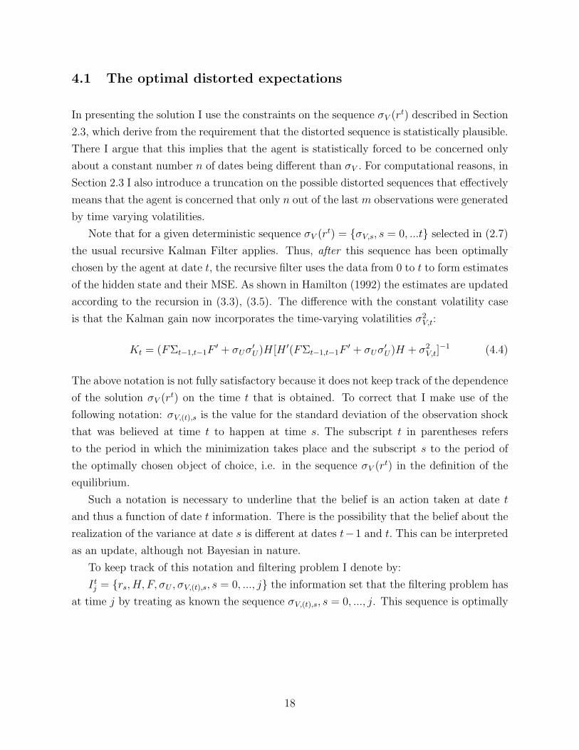
Note that for a given deterministic sequence σV (rt) = σV,s, s = 0, ...t selected in (2.7)

the usual recursive Kalman Filter applies. Thus, after this sequence has been optimally

chosen by the agent at date t, the recursive filter uses the data from 0 to t to form estimates

of the hidden state and their MSE. As shown in Hamilton (1992) the estimates are updated

according to the recursion in (3.3), (3.5). The difference with the constant volatility case

is that the Kalman gain now incorporates the time-varying volatilities σ2V,t:

Kt = (FΣt−1,t−1F′ + σUσ

′U)H[H ′(FΣt−1,t−1F

′ + σUσ′U)H + σ2

V,t]−1 (4.4)

The above notation is not fully satisfactory because it does not keep track of the dependence

of the solution σV (rt) on the time t that is obtained. To correct that I make use of the

following notation: σV,(t),s is the value for the standard deviation of the observation shock

that was believed at time t to happen at time s. The subscript t in parentheses refers

to the period in which the minimization takes place and the subscript s to the period of

the optimally chosen object of choice, i.e. in the sequence σV (rt) in the definition of the

equilibrium.

Such a notation is necessary to underline that the belief is an action taken at date t

and thus a function of date t information. There is the possibility that the belief about the

realization of the variance at date s is different at dates t−1 and t. This can be interpreted

as an update, although not Bayesian in nature.

To keep track of this notation and filtering problem I denote by:

I tj = rs, H, F, σU , σV,(t),s, s = 0, ..., j the information set that the filtering problem has

at time j by treating as known the sequence σV,(t),s, s = 0, ..., j. This sequence is optimally

18

selected at date t. Thus,

xti,j = E(xi|I tj)

Σti,j = E[(xti − xti,j)(xti − xti,j)′|I tj ]

Kti = (FΣt

i−1,i−1F′ + σUσ

′U)H[H ′(FΣt

i−1,i−1F′ + σUσ

′U)H + σ2

V,(t),i]−1 (4.5)

Thus xti,j is the estimate of the hidden state for time i based on the sample 0, ..., j by

treating as known the sequence σV,(t),s, s = 0, ..., j. This sequence is chosen at date t. Kti

is the Kalman gain to be applied at time i by using the known realization of σ2V,(t),i. This

value is an element of the sequence σV,(t),s, s = 0, ..., j.

In order to solve the problem in (2.7) and (4.1) I endow the agent with a guess about

the relationship between the future exchange rate and the estimates for exogenous process.

Similar to the RE case, I will restrict attention to linear function. Let this guess be

st+1 = Γxt+1t+1,t+1 + δrt+1 (4.6)

For the minimization in (2.7) the agent needs to understand how the expected utility

under the distorted model depends on σV (rt). For every possible σV (rt) the agent computes

the implied estimates and relevant state variables at time t+ 1. In comparing these cases,

the agent is using the guess in (4.6).

To understand the solution we could imagine an approximation of the per period felicity

function in (2.7) to U = − exp(−γEPt Wt+1 + γ2V arPt Wt+1). As done in the solution to the

portfolio choice problem, up to a second order, Wt+1 = btqt+1.

Thus, EPt Wt+1 = bt(E

Pt (st+1)− st − rt) and V arPt Wt+1 = b2

tV arPt st+1. Given the guess

in (4.6) and the Kalman filtering formulas

st+1 = Γ(I −Kt+1t+1H

′)Fxt+1t,t + (ΓKt+1

t+1 + δ)rt+1 (4.7)

The sequence σV (rt) does not affect the estimates xt+1t,t , K

t+1t+1 since these are formed based

on the optimal choice of the time t+ 1 agent.

4.1.1 Effect of the precision of signals on expected excess returns

Using (4.7), the exchange rate for the next period st+1 is monotonic in the realization of the

interest rate differential rt+1. More specifically, in equilibrium it is a decreasing function of

rt+1. The direction of the monotonicity is controlled by (ΓKt+1t+1 + δ) where Γ, δ are to be

19

determined in equilibrium. As expected, the same intuition about these parameters holds

as in the RE case. A positive realization for rt+1 will translate into an appreciation of the

domestic currency because the domestic interest rate is higher than the foreign one. Thus,

in equilibrium (ΓKt+1t+1 +δ) is a negative number. By this result, EP

t (st+1) is also decreasing

in EPt (rt+1).

The expected interest rate differential is given by the hidden state estimate EPt (rt+1) =

H ′Fxtt,t. This is clearly increasing in the innovation rt−H ′Fxtt−1,t−1. In turn, the estimate

xtt,t is updated by incorporating this innovation using the gainKtt . The latter is decreasing in

the variance of the temporary shock σ2V,(t),t. Intuitively, a larger variance of the temporary

shock implies less information for updating the estimate of the hidden persistent state.

Combining these two monotonicity results, the estimate xtt,t is increasing in the gain if the

innovation is positive. On the other hand, if (rt − Fxtt−1,t−1) < 0 then xtt,t is decreased by

having a larger gain Ktt .

By construction, expected excess return EPt Wt+1 is monotonic in EP

t (st+1). The sign

is given by the position taken in foreign bonds bt. If the agent decides in equilibrium to

invest in domestic bonds and take advantage of a higher domestic rate by borrowing from

abroad, i.e. bt < 0, then a higher value for EPt (st+1) will hurt her.

Proposition 1 Expected excess return, EPt Wt+1 is monotonic in σ2

V,(t),t. The monotonicity

is given by the sign of bt(rt −H ′Fxtt−1,t−1).

Proof. By combining the sign of the partial derivatives involved in∂EP

t Wt+1

∂σ2V,(t),t

. For details,

see Appendix C.

The impact of σ2V,(t),t on utility through the effect on the expected excess returns is

given by the following intuitive mechanism. Suppose in equilibrium the agent invests in

domestic bonds. She is then worried about a depreciation of the domestic currency, which

in equilibrium happens if the estimated hidden state of the differential xtt,t is lower, but

still positive. The variance σ2V,(t),t affects the gain Kt

t . To get a lower estimate xtt,t the

variance σ2V,(t),t is increased if the innovation (rt − Fxtt−1,t−1) is positive and is decreased if

the innovation is negative.

4.1.2 Effect of the precision of signals on expected variance of returns

The variance of excess returns is given by V arPt Wt+1 = b2tV ar

Pt st+1. In turn, using the

conjecture (4.7)and taking as given xt+1t,t , K

t+1t+1

V arPt st+1 = (ΓKt+1t+1 + δ)(ΓKt+1

t+1 + δ)′(V arPt rt+1) (4.8)

20

By the filtering formulas

V arPt rt+1 = H ′FΣtt,tF

′H +H ′σUσ′UH + EP

t (σ2V,t+1) (4.9)

In Appendix C.1 I discuss the object EPt σ

2V,t+1 and conclude that it is equal to (σHV )2 n

t+

(σV )2(1− nt). When t is large then this expectation becomes σ2

V .

Proposition 2 The expected variance of excess return, V arPt Wt+1 is increasing in σ2V,(t),t.

Proof. The variance V arPt Wt+1 is increasing in the conditional variance of the differen-

tial rt+1. By (4.9) the latter is increasing in σ2V,(t),t through the effect on Σt

t,t. For details

see Appendix C.

Intuitively, a larger variance of the temporary shocks translates directly into a higher

variance of the estimates Σtt,t. By choosing higher values of σV in the sequence σV (rt) she

will increase the expected variance of the differential V arPt rt+1 because∂Σt

t,t

∂σ2V,(t),t

> 0.

The overall effect of σ2V,(t),t on the utility Vt is then coming through two channels. One

is the positive relationship between σ2V,(t),t and the variance of the returns as in (4.8). As

shown above, σ2V,(t),t also influences Vt through the expected returns. The total partial

derivative is then

∂Vt∂σ2

V,(t),t

=∂Vt

∂EPt rt+1

∂EPt rt+1

∂σV,(t),t+

∂Vt

∂V arPt rt+1

∂V arPt rt+1

∂σV,(t),t

The sign of this derivative is :

sign(∂Vt

∂σ2V,(t),t

) = sign(bt)sign(rt − Fxtt−1,t−1)− sign(∂V arPt rt+1

∂σ2V,(t),t

)

From (4.9) the sign(∂V arP

t rt+1

∂σ2V,(t),t

) is positive. Thus, if the sign of [bt(rt − Fxtt−1,t−1)] is

negative the two effects align because a higher variance σ2V,(t),t will imply lower expected

excess returns. However, if the sign is positive the two directions are competing. To

analyze this situation I show in Appendix C that in this setup the probability that the

effect through the expected returns to dominate the one through the variance is almost

equal to 1. I conclude that in this model the effect of σV (rt) on utility goes through its

effect on expected returns.

The position bt dictates in what direction is the agent pessimistic. If, for example,

bt < 0 she invests in the domestic currency and is thus worried about a future domestic

depreciation. It is helpful to think about investing in a currency as buying an asset whose

21

payoff is the interest differential and whose capital gain is the appreciation of the currency.

In equilibrium the agent will essentially invest in the domestic currency if the domestic

interest rate differential is positive. The higher the differential the larger the demand for

this asset. The agent realizes then that this asset’s capital loss will be higher the less

agents will demand this asset in the next period. In equilibrium, the lower is the domestic

differential next period the less is the demand for this asset next period. Since the agent

is worried about capital losses when she considers investing in this asset, she in fact is

concerned that the domestic differential will be lower next period. The expectation about

this future differential is controlled by the estimate of the hidden state. Thus the agent

facing different possible DGPs fears that this estimate, although positive since she invests

in the asset, is lower than what the reference DGP implies.

To make the estimate of the hidden state of the domestic differential (xtt,t) lower, the

optimal sequence σ∗V (rt) involves choosing high values for σ2V,(t),s when the innovations

rt−s − Fxtt−s−1,t−s−1 are positive and low values when these innovations are positive. The

decision rule for choosing a distorted σV,(t),s is:

σV,(t),s = σHV if bt(rs − Fxts−1,s−1) < 0 (4.10)

σV,(t),s = σLV if bt(rs − Fxts−1,s−1) > 0

One way to interpret this sequence is that agents react asymmetrically to news. If the

agent decides to invest in the domestic currency then increases (decreases) in the domestic

differential are good (bad) news and from the perspective of the agent that wants to take

advantage of such higher rates. An ambiguity-averse agent facing information of ambiguous

quality will then tend to underweigh good news by treating them as reflecting temporary

shocks and overweigh the bad news by fearing that they reflect the persistent shocks.

In Section 2.3 I introduced the restriction that the agent only considers n dates out

of the last m to be different from the reference model. Out of these possible sequences,

the intuition given by (4.10) shows on what type of sequences the agent restricts attention

because they affect negatively her utility. The number of such possible sequences is the

choose function of m and n : mCn = m!/(n!(m − n)!). Out of these relevant sequences

the agent chooses the one that minimizes the estimate of the hidden state. If for example

m = n, as in the benchmark parameterization, nCn = 1 and the decision rule in (4.10)

implies the existence of only one such sequence. In the definition of the equilibrium I

denoted by σ∗V (rt) the solution to this minimization problem. This decision rule is taking

bt as given. The solution for this is similar to the RE case, except that the subjective

probability distribution for the future excess return is the one implied by the optimal

22

choice for σ∗V (rt) found above.

4.2 Numerical solution procedure

The driving equilibrium relation is the no-arbitrage condition given by the FOC with respect

to bt in (4.1). To solve that problem the agent needs to form forecasts about the next period

exchange rate. The conjecture in (4.6) is that st+1 = Γxt+1t+1,t+1 + δrt+1 so that forecasts of

xt+1t+1,t+1 and rt+1 are needed. At time t the agent knows the equilibrium updating rule for

time t+ 1:

xt+1t+1,t+1 = Fxt+1

t,t +Kt+1t+1(rt+1 −H ′Fxt+1

t,t )

The agent will use the decision rule for σV (rt+1) given by (4.10). For every possible

realization of rt+1 she will have to solve the agent’s time t + 1 problem, who will in that

case face the sample (rt, rt+1). For the resulting xt+1t+1,t+1 there will be a st+1 based on the

conjecture (4.6). This distribution of st+1 will imply the distribution for qt+1 = st+1−st−rtin (4.1). However, because of the asymmetric responses to innovations, normality is lost and

I did not find any closed-form solution to deal with it. Hence, to recover the distribution

for st+1 I perform the procedure numerically.

I restrict attention to linear time-invariant conjectures as in (4.6). Suppose first the

parameters Γ and δ are known. The solution to the distorted expectations equilibrium can

be summarized by the following steps.

1. Make a guess about the sign of bt to use in (4.10).

2. Use (4.10) and call the resulting optimal sequence σ∗V (rt). Use the Kalman filter

based on the sequence σ∗V (rt) to form an estimate for xtt,t and Σtt,t.

3. Draw realizations for rt+1 from N(H ′Fxtt,t, V arPt rt+1), where V arPt rt+1 is defined in

(4.9). Form the sample rt+1 = (rt, rt+1). For each realization perform Steps 1 and 2 above

to obtain the sequence σ∗V (rt+1).

4. For each realization in step 3 use σ∗V (rt+1) to compute xt+1t+1,t+1 and use the conjecture

in (4.6) to generate a realized st+1.

5. The distribution of st+1 in step 5 defines the subjective probability distribution for

the agent at time t. Use the FOC (4.1) to solve for s∗t .

6. If sign(s∗t ) = sign(bt) the solution is σ∗V (rt) and s∗t . If not, switch the sign in step 1.

7. If there is no convergence on the sign of s∗t and bt, the solution is assumed to be

b∗t = s∗t = 0.

The last point deserves some explanation. It is related to the Nash equilibrium solution

between the minimizing and maximizing player in (2.7). Consider the solution for the

23

sequence σ∗V (rt) that minimizes the utility. This solution needs to take as given an

investment position. When the guess is that the agent would like to invest in the seemingly

higher rate currency she will choose a sequence σ∗V (rt) to decrease the estimate of the

differential. If based on this worse-case scenario the solution to the portfolio choice is to

invest in the other currency it brings about a difficult situation for the agent. Initially she

considers investing in a currency but once she takes into account that the model might

be misspecified and uses the distorted model under this investment strategy her resulting

estimates make her want to invest in the other currency. If, when switching direction, the

same problem happens it means that there is no Nash equilibrium in pure strategies. I

do not consider mixed strategies and instead I impose the solution in these cases to be

bt = st = 0. These are situations in which the hidden state estimate of the differential is

very close to 0 under the true DGP and the uncertain averse agent is not willing to take

any side in the strategy. For this bt the agent does not invest in any bond so any solution to

σ∗V (rt) is a best response to bt. Note that the particular assumed solution for σ∗V (rt) does

not have any impact on the results since in the calculations of excess returns only periods

when bt is different from zero are considered. For future reference I call this situation the

“inaction” effect.

A concern is how to recover the parameters Γ and δ in the guess (4.6). The consistency

of beliefs in the definition of equilibrium (see Section 2.4) requires that the guess about

the law of motion be the correct relation on average. Because the distortions expectations

model is solved numerically, this consistency will require some approximations. I first start

by using the values for Γ and δ for the RE case. I find that the solution s∗t from the numerical

procedure and its implied value Γxtt,t + δrt by (4.6) are close. On average the difference

is 0 in long samples. Nevertheless, one could still expect that [s∗t − (Γxtt,t + δrt)]bt < 0

because the agent takes into account the asymmetric response to news for the next period.

For example, when bt < 0, that should bring the expected exchange rate slightly closer

to 0. Thus s∗t should be slightly higher than Γxtt,t + δrt. However, the “inaction” effect

mitigates this response. When bt < 0 the agent realizes that in equilibrium it is very

unlikely that st+1 > 0, i.e. that agents switch their position in the carry trade next period.

Realizations for rt+1 that would result under the rational expectations model in switching

investment positions are now most likely to be in the “inaction” region and be characterized

by st+1 = 0. A similar intuition applies for bt > 0. I find that the combined effect of these

two directions is that s∗t is close to Γxtt,t + δrt. The parameters Γ and δ that minimize

the distance between the two objects even in subsamples are characterized by a smaller

response of st to the estimate xtt,t. These parameters would correspond to the rational

expectations model solution if there would be less persistence in the hidden state.

24

The market clearing condition states that bt = .5st. In the RE case I approximated

logWt+1 by btqt+1. Then using the normality of qt+1 I obtained the mean-variance solution

in (3.1). In the distorted expectations model the excess return is no longer exactly normally

distributed. However, I find that numerically the mean-variance approximation to the bond

demand is very accurate. For intuition, I present this case and by using bt =EP

t (qt+1)

γV arPt (qt+1)

, I

get

st =EPt (st+1 − rt)

1 + .5γV arPt (st+1)(4.11)

I call (4.11) the UIP condition in the distorted expectations version of the model.

4.3 Options and risk neutral skewness

In this section I introduce options and define the risk-neutral probability distribution.

These elements are needed for contrasting the model’s implications against the data.

The asymmetric response to news that underlies the optimality of the distorted model

is generating in this model another interesting feature: the negative skewness of the carry

trade returns. This characteristic has sometimes been called “crash risk”. Burnside

et al. (2008), Brunnermeier et al. (2008) and Jurek (2008) find strong evidence of this.

Brunnermeier et al. (2008) argues that the mean profitability might be a compensation for

the negative skewness. They also note that the data suggests that the negative skewness is

endogenous. It is positively predicted by a larger interest rate differential. They argue that

the sudden unwinding of the carry trade positions causes the currency to crash. In their

view, the cause is liquidity shortages. In my model, the endogenous unwinding is caused

by asymmetric response to news.

For analyzing the model implied risk-neutral SkewPt,t+1 I use the numerical procedure

for solving the distorted expectations model and construct the distribution of excess returns

qt+1 = st+1 − st − rt based on her distorted model. This distribution is used by the agent

is solving for the optimal investment decision and thus generate the equilibrium exchange

rate. The risk neutral measure is implied by the FOC in (4.2): EPNt [qt+1] = EP

t

[dPN

dPqt+1

].

In the unhedged version of the carry trade presented above, the agent’s end-of-period

wealth is exposed to both upside and downside risk. Of particular concern is the possibility

of significant losses produced by large depreciations of the investment currency. To

eliminate the downside risk, an agent can use an option that provides insurance against

the left tail of the returns.

A call option on the FCU will give the agent the right but not the obligation to buy

foreign currency with domestic currency (USD) at a prespecified strike price kt dollars per

25

unit of FCU. Let C(kt) denote the price, including the time t interest rate, of the call option

with strike price kt. The net payoff in USD from investing in this option is25:

zCt+1(kt) = max(0, st+1 − kt)− C(kt)

Similarly, a put option on the FCU gives the agent the right, but not the obligation, to

sell foreign currency for USD at a prespecified strike price kt dollars per unit of FCU. Let

P (kt) denoting the price, including the time t interest rate, of the put option with strike

price kt. The net payoff in USD from investing in this option is:

zPt+1(kt) = max(0, kt − st+1)− P (kt)

Options are priced according to the no-arbitrage conditions:

C(kt) = EPt

[max(0, st+1 − kt)

µt+1

EPt µt+1

]

P (kt) = EPt

[max(0, kt − st+1)

µt+1

EPt µt+1

]

where µt+1 is defined in (4.3).

Options are used by the agent as protection against negative realizations. When she

decides to take advantage of the higher domestic interest rate by investing in the domestic

currency, she is worried about a pronounced depreciation of the domestic currency. In

that case her downside risk is eliminated by buying a call option on the FCU which pays

when st+1 is higher than the strike price kt. Similarly, when the agent invests in the foreign

currency she buys a put option on the FCU that pays when the foreign currency diminishes

in value, i.e. when st+1 is lower than kt.

The unhedged carry trade strategy means borrowing in the low interest rate currency

and investing in the high interest rate currency. The agents in the model use this strategy

in equilibrium. Their end-of-life wealth is given by bt(st+1−st−rt). By the market clearing

condition bt < 0 when st < 0.26 The payoff on a dollar bet for the unhedged carry trade

25The payoff should be expressed in terms of levels of the exchange rate as zCt+1(Kt) = max(0, exp(st+1)−

exp(kt)) − C(Kt). Using the approximation exp(x) − 1 ≈ x, when x is small, this becomes zCt+1(kt) =

max(0, st+1 − kt)− C(kt).26In simulations, the coefficient of correlation between st and rt is around −0.97. The correlation is not−1 because the exchange rate depends mostly on the sign of the hidden state estimate and this can bedifferent from the sign of the interest rate. Moreover, due to the “inaction” effect in some cases agentschoose not to invest at all if rt is too close to 0. In these few case I assume that the payoff to the carrytrade is 0.

26

strategy is:

zt+1 = rt − (st+1 − st) if bt < 0 (4.12)

zt+1 = (st+1 − st)− rt if bt > 0

Then I define the return to the hedged carry trade, zHt+1, as the sum of the payoff to the

unhedged carry trade and from buying an option at strike price kt corresponding to the

strategy of eliminating the downside risk :

zHt+1(kt) = zt+1 + zCt+1(kt) if bt < 0 (4.13)

zHt+1(kt) = zt+1 + zPt+1(kt) if bt > 0

where zt+1 is the payoff to the unhedged carry trade defined in (4.12).

4.4 Parameterization

In the benchmark case, the reference model is a state space representation with constant

volatilities as in (2.1). I estimate the relevant parameters by using Maximum Likelihood

on data on interest rate differential. The data set is obtained from Datastream and

consists of daily observations for the mean of bid and ask interbank spot exchange rates,

1-month forward exchange rates, and 1-month interest rates. I convert daily data into

nonoverlapping monthly observations. The data set covers the period January 1976 to

December 2006 for spot and forward exchange rates and January 1981 to December 2006

for interest rates. The countries included in the data set are listed in Table 10.

Table 11 reports results for the Maximum Likelihood estimation of (2.1) on interest rate

differential data. First, I find a very high degree of persistence in the state evolution. The

table reports values for the long-run autocorellation of the hidden state, denoted by∑ρ,

which is defined as the sum of the AR coefficients for the transition equation. Second, I

find evidence for a positive σV with some heterogeneity in its statistical significance.27 The

benchmark parameterization is a version of (2.1) which averages across these heterogeneity.

In robustness checks I also use the other available data and find that the main conclusions

hold. The results would be significantly weaker in the case in which the true σV would be

several times larger than σU . I discuss this implication in Section 5.1.

27Performing a similar exercise, Gourinchas and Tornell (2004) find that there is no evidence of a positiveσV in the interest rate differential data they analyze. There the sample is 1986-1996. I find that by includingearlier data, which is characterized by more sudden movements, the evidence becomes stronger in favor ofa positive σV .

27

For the state space defined in (2.1) H ′ = [1 0 0 0], σU = [σDGPU 0 0 0] and

F =

ρ1 ρ2 ρ3 ρ4

1 0 0 0

0 1 0 0

0 0 1 0

Table 2 reports the benchmark parameterization.

Table 2: Benchmark specification

σV σHV σLV σDGPU ρ1 ρ2 ρ3 ρ4 γ0.00025 0.0037 0.000166 0.0005 1.54 −0.52 −0.34 0.3 10

These values imply that the steady state Kalman weight on the innovation used to

update the estimate of the current state is 0.86, 1 and 0.17 for the true DGP, the low

variance and the high variance case. Although the lower gain might seem very different

than the true DGP, note that the model does not imply that these gains are used for every

period. It is only for a few dates in a large sample that such distorted gains are employed.28

As discussed in Section 2.3 in order for the equilibrium distorted sequences of variances

to be difficult to distinguish statistically from the reference sequence I restrict the elements

in the alternative sequences considered by the agent to be different from the reference model

only for a constant number n of dates. As introduced in Section 2.3 for computational

reasons I also make a restrictive assumption about the distorted sequence so that at time

t the agent considers the n points of possible distortions only for dates t−m+ 1 through

t. To quantify the statistical distance between the two models I use a comparison between

the log-likelihood of a sample rt computed under the reference sequence (LDGP (rt)) and

under the distorted optimal sequence (LDist(rt)).

Table 3 reports some statistics for the likelihood comparison LDist(rt) − LDGP (rt),

computed for a sample of T = 300, for various cases. The Table reports the mean

average and the standard deviation of this difference and the percent of times for which

this difference is positive. The standard deviation of these statistics is then computed

accross the N = 1000 simulations. Column (1) reports the results for the benchmark

parameterization in which m = n = 2. It also shows that for about 17% of cases LDGP (rt)

28Also note that when a distortion is occurring the Kalman gain does not instantly adjust to thesteady gain but it evolves according to the deterministic chosen sequence of variances. With time-varyingvolatilities in the observation equation, such adjustments are nevertheless quick.

28

Table 3: Likelihood comparison: LDist(rt)− LDGP (rt)

(1) (2) (3)Mean −1.48 −1.39 −138

(0.06) (0.05) (3.2)St.dev. 1.13 1.06 3.2

(0.03) (0.03) −%positive 0.167 0.178 0

(0.021) (0.027) −

is smaller than LDist(rt). This statistic is referred to as the probability of model detection

error. Column (2) reports these values for the case in which n = 2 and m = 10. The

results are very similar to the benchmark specification with the LDist(rt) being slightly

higher on average in this case. Column (3) considers the situations in which there is no

restriction on the number of periods for which the agent distorts the sequence so that any

previous period characterized by good news is attached a low precision of signals and bad

news a high precision of signals. In this case n = t and the difference LDGP (rt)− LDist(rt)is increasing with the sample size. For T = 300 the average difference accross simulations

is around 170 log points. Thus, such a distorted sequence would result in an extremely

unlikely interpretation of the data. For this reason, I restrict n to be a small number.

The parameters δ,Γ, σ2 that characterize the solution to the rational expectations model

are given by equations (3.7), (3.8) and (3.9) respectively. As mentioned in Section 4.2 for the

distorted expectations model I need to use a numerical approach to finding the equilibrium.

I find that a good approximation is that the δ,Γ, σ2 can be computed using the same

equations but with a slightly less persistence in the state-equation. Thus, I compute these

parameters for an F that differs from F above in its first component: F (1, 1) = 1.538.

The intuition why the numerical procedure delivers such a result is that in the distorted

expectations model the exchange rate in fact responds less to the same state variables as in

the rational expectations case. This response is controlled by the persistence of the state

equation. A larger maximal eigenvalue for F produces a larger eigenvalue for Γ.

For the absolute risk aversion parameter γ I use in the benchmark parameterization a

value of 10. A higher value allows for risk aversion to play a slightly larger role, given the

known extreme sensitivity of portfolio choice to expected excess returns in this setup. In

fact, I find in robustness checks that as long as γ is in a standard range the main results

are insensitive to its value.

29

5 Results

In this section I present the main implications that the distorted expectations model has

for exchange rate puzzles. Figures 1 and 2 illustrate for one simulation of the model the

exchange rate path and the estimate of the hidden state of the domestic interest rate

differential under the distorted expectations version and the rational expectations (RE)

version. For comparison, the same exogenous driving process is used but the estimates are

computed under the different model solutions. When the agent is investing in the foreign

bond, i.e. bt > 0 and st > 0 , she is concerned that the negative estimate of the hidden

state is in fact less negative than what the reference model would imply. Her investment

position will reflect her pessimistic assessment of the future distribution and she will invest

less compared to the RE model. Thus st < sREt when st > 0 and st > sREt when st < 0

where sREt denotes the exchange rate under RE.

Figure 1: Model generated exchange rate path

50 100 150 200 250 300

−0.1

−0.05

0

0.05

0.1 AmbiguityRational Expectations

Table 4: Correlations exchange rates

(1) (2) (3) (4)0.96 0.26 0.164 0.356

(0.02) (0.04) (0.04) (0.05)

Figure 1 shows that the exchange rate under ambiguity is reacting asymmetrically to

news. When for example bt < 0 the domestic currency appreciates more gradually while

30

depreciating suddenly compared to its RE version. This is consistent with the description

that for the high interest rate (investment) currency “exchange rates go up by the stairs

and down by the elevator” (see Brunnermeier et al. (2008)). To investigate this asymmetric

response further, Table 4 computes correlations between the exchange rate under ambiguity

and under RE. The unconditional correlation in levels is very high while in first differences

is lower. Columns (3) and (4) indicate that conditional on states in which the investment

currency tends to appreciate the correlation in first differences is much weaker than in

states in which the investment currency is depreciating.

For the same simulation that generated the exchange rate path in Figure 1, Figure 2

illustrates the estimate of the hidden state of the domestic differential. The same intuition

regarding the asymmetric response applies here. Table 5 shows that the correlation between

the estimate in first difference under ambiguity and under RE is much weaker when the

interest rate of the investment currency tends to increase compared to states in which this

interest rate decreases.

Figure 2: Model generated estimates of hidden state

0 50 100 150 200 250 300−4

−3

−2

−1

0

1

2

3

4

5x 10

−3

AmbiguityRational Expectations

Table 5: Correlations estimate of hidden state

(1) (2) (3) (4)0.97 0.49 0.35 0.69

(0.02) (0.05) (0.04) (0.06)

In terms of other conditional relationships I find that a higher domestic interest rate

31

differential: 1) does not predict on average a larger domestic currency depreciation. The

UIP regression coefficient is on average negative, not significantly different from zero in

small samples, but significantly negative in large samples; 2) predicts a positive excess

return from the unhedged carry trade strategy; 3) predicts a positive excess return from the

hedged carry trade strategy; 4) predicts a negatively skewed excess return for the unhedged

carry trade strategy; 5) is associated with a more negative risk-neutral skewness of expected

excess returns; 6) is followed by a gradual appreciation of the domestic currency.

5.1 The UIP puzzle and positive unhedged carry trade returns

In the distorted expectations model a risk adjusted version of UIP holds ex-ante and the

expected excess returns under the risk neutral measure are zero (see (4.2)). The UIP

regression is:

st+1 − st = βrt + εt+1 (5.1)

In the distorted model, with µt+1 = exp(−γbtqt+1) denoting the marginal utility and

λt+1 =µt+1

EPt µt+1

, the expected exchange rate difference equals

EPt (st+1)− st = EP

t (st+1)− EPt [st+1λt+1] + rt

If the true DGP is the distorted model then EPt (εt+1|It) = 0 and

β = 1 +cov(cov(st+1λt+1), rt)

var(rt)

The message of the time-varying risk premia story is that the term cov(cov(st+1λt+1),rt)var(rt)

cannot deliver a significantly β < 1. If the true DGP is the distorted model, the results

established for the rational expectations apply here too except that the log excess return is

not normally distributed. However, as I presented before, I find numerically that the mean

variance result is a very good approximation for the optimal bond solution which delivers

EPt (st+1)− st = EP

t (st+1)− EPt (st+1 − rt)

1 + .5γV arPt (st+1)

As explained at length in the RE case, the conditional variance V arPt (st+1) has a very

small effect in obtaining a coefficient smaller than 1. In the distorted expectations model,

the same result applies, with the observation that V arPt (st+1) is even slightly lower given

the implied smaller response of the exchange rate to the fundamentals. For reasonable

values of γ the lower bound on β would be also around 0.999. Hence in presenting the

32

Table 6: Model implied β for the UIP regression

(1) (2) (3) (4) (5)

β tβ β tβ β tβ β tβ β tβT=300 Mean -0.25 -0.81 0.37 1.27 0.34 1.1 -0.57 -1.1 -0.19 -0.68

Median -0.22 -0.76 0.32 1.24 0.28 0.95 -0.55 -0.93 -0.17 -0.65St.dev. 0.14 0.3 0.22 0.51 0.21 0.36 0.24 0.47 0.11 0.28

T=3000 Mean -0.28 -2.14 0.54 1.75 0.48 1.58 -0.66 -2.58 -0.21 -1.71Median -0.28 -2.14 0.52 1.72 0.47 1.55 -0.67 -2.59 -0.21 -1.71St.dev. 0.07 0.27 0.11 0.32 0.09 0.2 0.11 0.27 0.06 0.25

results I will make use of the fact that the 1 + .5γV arPt (st+1) is approximately equal to

1. In a richer environment the ambiguity aversion theory presented in this paper can be

incorporated into models that take more seriously the risk premia corrections. With the

covariances becoming effectively zero the risk neutral UIP implies that if the true DGP is

the distorted model then β = 1 since EPt (st+1)− st = rt.

If the DGP is different from the distribution implied P the coefficient β can be

significantly lower than 1. The focus of this paper is to show that a model with ambiguous

precision of signals about a time-varying hidden state can provide an explanation for a

negative β. Table 6 presents the estimated β for the model implied UIP regression in (5.1)

in 1000 repeated samples of T = 300 and 500 repeated samples of T = 3000. Column

(1) is the benchmark specification and shows that, for small T , the model is generating

a negative average β, even if not significant statistically. As the sample size is increased

and the standard errors reduce, the average and median estimate become significant. This

highlights that the results of the model are not limited to small sample and in fact are

stronger in large samples. The type of ambiguity modeled in this paper is active even as

the sample size increases.

Figure 3 is the histogram of the UIP coefficients across many repeated samples. The

top panel plots the histogram of the estimated UIP coefficients on N = 1000 samples of

T = 300. It shows that the vast majority of the estimates are negative. For the large sample

of T = 3000 the bottom panel of Figure 3 indicates the distribution of the estimates and

shows that there are no positive values obtained.

Column (2) of Table 6 considers a case in which the noise-to-signal ratio in the true DGP

is much higher than in the benchmark model. In that case, the estimated UIP coefficient

is positive. For that parameterization the steady state Kalman gain for the true DGP,

high distorted precision and low distorted precision are 0.3, 0.95 and 0.03 respectively. The

33

Figure 3: Model implied UIP coefficients

−1.2 −1 −0.8 −0.6 −0.4 −0.2 00

50

100

150

200

250

300

350

Small sample

−0.4 −0.35 −0.3 −0.25 −0.20

20

40

60

80

100

120

140

Large sample

Kalman gain used by the agent in updating the estimated hidden state is time-varying

to reflect the optimal response of the agents to “good” and “bad” news. This optimal

time-variation implies two opposing forces on β: the underreaction makes the coefficient

become negative and the overreaction effect pushes it to be larger than 1. The combined

effect depends on how far apart are the distorted gains from the one implied by the true

DGP. In the benchmark case, as reported in Table 2, the true noise-to-signal ratio is small.

In that case the overreaction channel is dominated because the Kalman gain implied by

σLV is closer to the reference model. Intuitively, if σV is close to 0 any σLV < σV will make

a small difference on the implied gain. However, if σHV > σV the distorted gain can be

considerably smaller. In the variant reported in Column (2) the gain under the reference

model is closer to the one implied by σHV , so the underreaction effect is less active. That is

the reason why the estimated UIP coefficient is positive.

Column (3) of Table 6 shows that when there is significantly less persistence in the state

evolution the model cannot account for the UIP puzzle. For that experiment the long run

autocorrelation of the state is 0.7. The reaction of the exchange rate to the estimate of

the hidden state is strongly affected by this persistence because the present value of future

payoffs to a bond is smaller following the same increase in the interest rate. For the same

interest rate differential this makes agents demand less of the bond and the investment

currency value goes up by less. As Engel and West (2004) argue, for a high persistence

34

of the fundamentals the exchange rate is very sensitive to changes in the present value of

future payoffs. They argue that this explains why exchange rates are hard to predict even

in a model where they are completely determined by fundamentals. A large sensitivity of

the currency’s value to the hidden state allows small distortions to the estimate to produce

large deviations in the exchange rate evolution. With significantly less persistence the

model has a difficult time in explaining the UIP puzzle.

These exercises show that the two main features of the true DGP that are required

for the theory to succeed are relatively small temporary shocks and large persistence of

the hidden state. The benchmark parameterization is characterized by these conditions

because the data strongly suggests such a calibration. It is important to note though that

Columns (2) and (3) of Table 6 show that the benchmark calibration is in fact rather robust

to changes as significant variations have to be made to it to reverse the results.

Column (4) of Table 6 presents the results for the parameterization of the model in

which there are no restrictions on the number of periods in which the agent can distort

the reference sequence, i.e. n = t. For such a case, the model implies a larger negative

Fama regression coefficient both in short and large samples. Thus, relaxing the benchmark

restrictions of n < t improves the model’s ability to generate the empirical puzzles at the

cost of implying very unlikely distorted sequences compared to the reference model. As

Column (3) of Table 3 reports, this case generates sequences that become increasingly less

likely as the sample size grows.

In the benchmark parameterization I also make an assumption about the number m

described in Section 2.3 and 4.4. This number effectively constrains the agent to only

consider n dates out of the last m to be different from the reference model. I investigate

this assumption by solving for the optimal distorted sequence when m = 10. As the original

motivation for having a lower m suggests, I am not able to simulate the future distribution

of exchange rates for this high m due to computational intensity. I find that when m = 10

the optimal dates chosen by the agent are very close to time t. The model can be simulated

to investigate the UIP coefficient by using the equilibrium relation for the exchange rate

in (4.6). I find, as reported in Column (5) of Table 6 that for m = 10 the results are

slightly weaker. As Column (2) of Table 3 shows, the error detection probability is also

relatively larger suggesting that setting m = 2 imposes additional statistical penalty on

the distorted sequence. Thus, compared to m = 10, in the benchmark case of m = 2

the model implies that the agent is using a distorted sequence that is generating slightly

stronger results for the UIP puzzle while being slightly easier to distinguish statistically

from the reference sequence. I find this result intuitive and conclude that the benchmark

specification provides results that are robust to the assumption of m = 2.

35

Figure 4: Model generated carry trade payoffs

−0.06 −0.04 −0.02 0 0.02 0.040

2

4

6

8

10

12

14x 10

4 Unhedged Carry trade payoffs

−0.03 −0.02 −0.01 0 0.01 0.02 0.03 0.04 0.050

2

4

6

8

10

12

14

x 104 Hedged Carry trade payoffs

Table 7: Model implied statistics for the unhedged carry trade returns

Mean Standard Sharpe Skewness KurtosisDeviation Ratio

T = 300 0.0017 0.0106 0.16 −0.421 5.37(0.0005) (0.007) (0.047) (0.288) (0.91)

T = 3000 0.0018 0.0115 0.1565 −0.19 6.58(0.0001) (0.00045) (0.01) (0.15) (0.68)

The payoff on a dollar bet for the unhedged carry trade strategy is defined in (4.12).

The model implied non-annualized monthly carry trade returns are described in Table 7.

They are characterized by a positive mean, negative skewness and excess kurtosis. The

excess returns have a positive mean because a high interest rate differential predicts on

average a zero currency depreciation or even a slight appreciation. The average mean

payoff reported in Table 7 is 0.0017. For the data analyzed in Table 10 the average mean

payoff for the carry trade strategy is 0.0033. This does not take into account transactions

costs. Burnside et al. (2008) (henceforth BEKR) analyze a more extensive data set and

find that the average payoff to the carry trade without transactions costs across individual

country pairs for the period 1976: 2007 ranges from 0.0026 when the base currency is the

GBP to 0.0042 when the base currency is the USD. With transaction costs they report

36

a range of 0.0015 to 0.0025. Table 7 also shows that the average standard deviation of

the model implied unhedged carry trade payoffs is around 0.011. For the data analyzed in

Table 10 the average standard deviation is 0.03. BEKR report average values ranging from

0.028 to 0.031.

Thus, compared to empirical evidence on the unhedged carry trade payoff, my model

delivers mean returns that are around half of those computed without transaction costs

and at the lower bound of the empirical payoffs with transaction costs. The model implied

average standard deviation of these payoffs is about a third of its empirical counterpart.

Naturally, the model is characterized by higher Sharpe ratios than in the data due to the

considerably lower standard deviation. The average Sharpe ratio for the model is 0.16 while

empirically BEKR find an average value around 0.1.

Figure 4 plots the histogram of the realized unhedged carry trade returns obtained for

N = 1000 samples of size T = 300. The mean of these returns is positive and compared to

a normal distribution with the same mean and variance the returns are negatively skewed

and have significant excess kurtosis.

5.2 Negative skewness and excess kurtosis of unhedged carry

trade returns

The results reported in Table 7 indicate that the returns to the carry trade are on average

negatively skewed. The degree of skewness is slightly larger than the one found in the data

for the carry trade returns analyzed in Table 10. The model implies a negative skewness

of -0.42 while the average for the countries in Table 10 is -0.24. BEKR report an average

for the individual country pairs of around -0.26.

To investigate the properties of the realized skewness of excess returns I construct the

following tests. The first, more cross-sectional in nature, is similar to that of Brunnermeier

et al. (2008). It involves checking whether periods (countries in Brunnermeier et al. (2008))

characterized by a higher domestic currency also experience a negative skewness in the

excess returns. To that end, I simulate the model for T = 300 and for each t collect rt and

the realized ext+1 = rt− (st+1− st). I sort the excess returns ext+1 according to the sign of

rt. Denote by ex+t+1 the returns when rt > 0 and by ex−t+1 when rt < 0. Consistent with the

predictability of excess returns the average of ex+t+1 is positive and the average of ex−t+1 is

negative. Importantly I find that the skewness of ex+t+1 is negative (-0.4) and that of ex−t+1

is positive (0.4).

A test for a time varying dimension is to simulate the model and at each date t to have

37

Table 8: Model implied statistics for the “crash risk” regressions

T = 300 T = 3000

β2 tβ2β3 tβ3

β2 tβ2β3 tβ3

−3.1 −8.61 −0.72 −10.21 −2.96 −7.83 −0.83 −12.41(1.21) (2.44) (0.29) (2.1) (0.89) (1.48) (0.22) (1.9)

N = 20000 draws from the DGP process for the date t+1 realizations of rt+1.This is similar

to the numerical procedure used to solve the distorted model but here the draws are from

the DGP and not from the subjective distribution. Using these draws I solve the model

at time t+ 1 and then collect the equilibrium implied st+1. Based on these I compute the

realized excess returns ext+1 = rt − (st+1 − st) and their skewness denoted by Skewt+1.

The same conclusions hold: a higher rt predicts a lower Skewt+1. Positive rt are associated

with negative Skewt+1. Table 8 reports the results of the regression

Skewt+1 = β2rt + ξ2,t+1

The model generates a negative significant β2 as found empirically by Jurek (2008) who

investigates both the cross-section and the time variation and finds that in both dimensions

the effect is very significant.

Consistent with the data, this implies that investing in a higher interest rate currency

produces an average positive excess return which is negatively skewed. The thicker left

tail occurs because of the larger reaction to negative innovations and smaller reaction to

positive shocks the excess returns are negatively skewed. Thus “crash risk” in this model

is endogenous and it happens when negative shocks hit an otherwise positive estimate of

the hidden state.

To study the properties of the agents’ expectations, Jurek (2008) computes the risk-

neutral implied skewness from options data. In my setup that corresponds to the object

SkewPt,t+1, defined in Section 4.3. It is worth noting again that the essential difference

between the risk-neutral and the realized probabilities is not the risk correction from

marginal utilities, but the distorted probabilities. This is at the heart of the mechanism of

the paper.

Table 8 also reports results for the regression

SkewPt,t+1 = β3rt + ξ3,t+1

38

Table 9: Model implied statistics for the hedged carry trade returns

Mean Standard Sharpe Skewness KurtosisDeviation Ratio

T = 300 0.0012 0.0067 0.179 1.46 7.22(0.0004) (0.0006) (0.038) (0.38) (1.81)

T = 3000 0.0012 0.0073 0.164 2.63 12.01(0.0001) (0.00037) (0.0135) (0.17) (1.66)

The model implied β3 is also negative and very significant. Thus there is a negative

correlation between the high interest rate differential and the skewness of the excess returns

under the distorted model. Again, this happens because agents take into account the

asymmetric response to news for the next period and thus expect a skewed distribution.

This negative relation is also present when the test is cross-sectional, as with the realized

skewness. Jurek (2008) also confirms this cross-sectional implication, i.e. periods of

higher domestic rate are also characterized on average by a negative risk-neutral skewness.

Interestingly, comparing the point estimates of β2 and β3 a higher rt has a larger conditional

impact on the predicted realized skewness than on the risk-neutral skewness.

5.3 Positive hedged carry trade returns and options

To measure the hedged carry trade I use the definition in (4.13) and as in BEKR I use

at-the-money options by setting kt = st. Table 9 presents the results for the hedged carry

trade. The average payoff is around 0.0012 which is smaller than the payoff for the unhedged

carry trade. BEKR also find this relation in the data. The standard deviation of the hedged

carry trade is lower and the resulting Sharpe ratio is slightly higher than for the unhedged

carry trade.

For intuition, take the case of the foreign currency being at a forward premium, i.e.

rt > 0 and st < 0. Buying a call option on the FCU is relatively expensive because the

probability of exercising the option is relatively large. By using the distorted model, the

agent believes that there will be a more depreciated domestic currency than what actually

happens at time t+ 1. This intuitively means that buying a call option delivers losses ex-

post. If one compares the average means of the payoffs, the average loss from buying the

insurance options is about 30% of the unhedged payoff consistent with findings in Jurek

(2008).29 BEKR report values that imply that the average individual country pair loss

29Jurek (2008) uses a more complicated version of hedging that also takes into account the delta exposure

39

resulting from eliminating the downside risk is about 20% of the unhedged payoff. Because

these losses are not that large the hedged carry trade still has positive average returns.

A way to think about the reason why the model generates positive average payoffs both

for unhedged and hedged strategies is to note that the subjective probability distribution

differs from the objective one by overpredicting bad events and underpredicting good events.

Buying insurance against the downside risk produces on average losses because of the

exaggeration of the probability of bad states under the subjective probability distribution

for the exchange rate realizations. However, the hedged position delivers positive payoffs

because of the more frequent occurence of the good events under the objective probability

distribution than under the equilibrium distorted beliefs.

The theory proposed here does not rely on a peso event explanation in the sense used

in the literature.30 Such an event is interpreted to be one that does not materialize in

the sample but is characterized by some extreme negative effect on the agent’s utility. As

BEKR point out this extreme negative event could be a large loss from the strategy or a

very high marginal utility when an otherwise small loss happens. To see the reasons why

the peso problem can explain the positive payoffs to the unhedged carry trade notice that

ex-ante the investor has to be compensated for this negative possibility. When this event

does not happen in the sample then ex-post the payoffs look systematically positive. If the

peso event is associated with a large loss this would necessarily mean that the hedged carry

trade would have zero payoffs. In that case buying an option as insurance against downside

risk should be producing systematic negative payoffs that outweigh exactly the gains from

the unhedged carry trade. They then conclude that it must be the extremely high marginal

utility that characterizes such a negative event. Clearly, in my model I cannot provide such

a solution.

The peso explanation assumes that the only difference between the subjective and the

objective distribution is the small probability rare disaster event that does not materialize

in the sample under the latter distribution. The mechanism presented here delivers a

realized distribution for the exchange rates that can have a different shape than the

subjective. Unlike the peso problem, there is no reasons to expect that any property

of these distributions is the same. Their mean are not equal thereby generating the ex-post

profitability of the unhedged carry trade. They are both negatively skewed and have excess

kurtosis. As explained above the model can deliver an explanation for the small losses of

buying insurance against the downside risks and implicitly for the positive payoffs of the

of the option.30This explanation has been put forward by recent papers such as Farhi and Gabaix (2008). In their

model there is a rare disaster that can happen with a small, time-varying probability.

40

hedged strategy because of the properties of these distributions.

5.4 Delayed overshooting

The forward premium puzzle refers to the unconditional empirical failure of UIP. This does

not necessarily imply that a conditional version of UIP fails too. Following a positive shock

to the interest rate the UIP condition states that the domestic currency should appreciate

on impact and then follow a depreciation path. Such a mechanism can be investigated

empirically by identifying the response of the exchange rate to a monetary policy shock.

Several studies have analyzed this conditional UIP using different identification restric-

tions. Eichenbaum and Evans (1995), Grilli and Roubini (1996) use short-run restrictions

to identify the effect of structural monetary policy shock on the exchange rate. They

find significant evidence of delayed overshooting: following a contractionary monetary

policy shock the domestic interest rate increases and there is a prolonged period of a

domestic currency appreciation. The peak of the impact occurs after one to three years as

opposed to happening immediately as predicted by the Dornbusch (1976) overshooting

model. Faust and Rogers (2003) find that these results are sensitive to the recursive

identification assumptions and that the peak of the exchange rate response is imprecisely

estimated. Scholl and Uhlig (2006) use sign restrictions and also find evidence for delayed

overshooting. For the country pairs they analyze the estimated peak occurs within a year or

two. Although they differ in their estimates of the length of the delayed overshooting effect

all these identifying approaches reach a robust conclusion: following a monetary policy

shock there are significant deviations from the UIP.

As discussed in Section 1, the model presented in this paper attempts to explain the

delayed overshooting puzzle through a mechanism similar to Gourinchas and Tornell (2004).

There they posit that if agents, for some reason, systematically underreact to news that

can explain the conditional and unconditional UIP puzzles. The difference is that here I

investigate a model which addresses the origin and optimality of such beliefs. As explained

in previous sections I find that agents underreact to good news and overreact to bad news.

However, for the impulse response function that I analyze and that is typical to the empirical

identification, it is only the underreaction effect that shows up, which makes the intuition

of the delayed overshooting similar to the one exposed in Gourinchas and Tornell (2004).

To generate the impulse response of the exchange rate to a shock to the interest rate

differential, assume that the economy starts in steady state. Thus, rt−1 = 0, bt−1 = 0,

EPt−1st = EP

t−1st = 0. At time t there is a positive shock to the interest rate differential.

To allow for a clearer intuition I present the case in which the transition equation is an

41

AR(1). The autocorrelation coefficient is equal to the largest eigenvalue of the matrix F

in the benchmark parameterization (see Section 4.4). Thus, I use the DGP

rt = xt + σV vt (5.2)

xt = ρxt−1 + σUut

where ρ = 0.9718. The values for σV and σU are the same as in Section 4.4.

To investigate the average response to an increase in rt this experiment needs to impose

that the observed positive shock to rt is generated by a combination of a shock to the

persistent and the temporary component that corresponds to their true DGP likelihood of

occurrence. Let vt = ut = 1. Then rt = σU + σV and xt = σU . The next periods shocks are

set equal to zero. The rational expectations (RE) solution is then: sREt = ΓRExREt,t + δRErt

and the distorted expectations solution is st = Γxtt,t + δrt, where xREt,t is the estimate of the

hidden state xt under RE and xtt,t is the estimate under the ambiguity aversion model. A

feature of this experiment is that xREt,t = xt while xtt,t 6= xt.

Figure 5 plots the dynamic response of the exchange rate to the observed increase in

rt. The RE version features the Dornbusch (1976) overshooting result in which the peak of

the impact is at time t. Consider the decision at time t. The agent sees the increase in the

interest rate differential but she is worried about a significant depreciation at time t + 1.

In equilibrium that means she is concerned that this rise in rt is caused by a temporary

rise. She then believes that the true σV,t = σHV and acts on this belief by investing much

less in the domestic bond than she would under rational expectations. By underestimating

the true hidden state she observes a higher than expected rt+1. Her updated estimate at

time t+ 1 is:

xt+1t+1,t+1 = ρxt+1

t,t +Kt+1t+1(rt+1 − ρxt+1

t,t )

In this setting xt+1t+1,t+1 is higher than xtt,t and a further appreciation occurs. Because

rt−ρxt−1,t−1 > 0 and using the notation I introduced in Section 4.1, σV,(t+1),t = σV,(t+1),t+1 =

σHV . At time t + 2 if the agent can distort only the last 2 periods as in the benchmark

specification then σV,(t+2),t = σV and σV,(t+2),t+1 = σV,(t+2),t+2 = σHV . This corresponds to

setting m = n. If m is allowed to be significantly larger than n so that if the agent distorts

2 periods but chooses what exactly these are, then I find that σV,(t+2),t = σV,(t+2),t+2 = σHVand σV,(t+2),t+1 = σV . If there is no restriction on n, so that the agent can distort any

period then σV,(t+2),t = σV,(t+2),t+1 = σV,(t+2),t+2 = σHV . A similar argument applies for

future periods. Eventually, the estimate of the hidden state converges to the RE case.

The top plot in Figure 5 shows the evolution of st in the benchmark specification in

42

Figure 5: Delayed overshooting

2 4 6 8 10 12 14 16 18 20−0.02

−0.015

−0.01

−0.005

0

AmbiguityRational expectations

2 4 6 8 10 12 14 16 18 20−0.02

−0.015

−0.01

−0.005

0

AmbiguityRational expectations

5 10 15 20 25 30 35 40 45 50−0.02

−0.015

−0.01

−0.005

0

AmbiguityRational expectations

which the agent distorts the sequence σV (rt) only for n = 2 periods and m = n. There the

peak occurs 2 periods later than in the rational expectations model. There is a gradual

appreciation until period 3 followed by a depreciation after the estimates of the hidden state

converge under the distorted and rational expectations. Note that for all cases in Figure

5 even after converging the exchange rate under ambiguity and RE differ slightly because

of the lower weight put on the estimate of the hidden state in the former. The second plot

shows the evolution under the specification of n = 2 periods but m = 10. In that case the

peak is 3 periods later. The bottom plot is one in which there is no restriction on n, i.e.

n = t. The agent can distort any period of the sample she observes and in this case she does

so by choosing a low precision of the signal for every period. In this case the appreciation

is much more gradual and the peak is 17 periods later than the time of the shock. This

plot also reproduces the intuition for the persistent delayed overshooting in Gourinchas

and Tornell (2004). However, as I argued in the discussion on the statistical plausibility

of the distorted sequences such a specification implies a very unlikely interpretation of the

observed sample. In fact, as the sample size increases such distorted sequences generated

likelihoods that become increasingly lower than the ones under the reference model.

The conclusion from Figure 5 is that the model can generate qualitatively the delayed

overshooting implication. The benchmark specification implies a quick peak and a short-

lived deviation from UIP because the agent is limited in distorting the time-varying

precision of signals by statistical plausibility considerations. When these considerations

are absent, the model delivers significantly longer delayed overshooting.

43

6 Conclusions

This paper contributes to the theoretical literature that attempts to explain the

observed deviations from UIP through systematic expectational errors. Such an approach

is motivated by the empirical literature based on survey data for the foreign exchange

market that finds significant evidence against the rational expectations assumption and

the empirical research that challenges the time-varying risk assumption.

I present a model of exchange rate determination which features signal extraction by an

ambiguity averse agent that is uncertain about the precision of the signals she receives. In

deciding on the optimal investment position the agent is estimating the time-varying hidden

state of the exogenous observed interest rate differential. In equilibrium the agent invests in

the higher interest rate currency (investment currency) by borrowing in the lower interest

rate currency (funding currency). The agent entertains the possibility that the data could

have been generated by various sequences of time-varying signal to noise ratios. Faced with

uncertainty agents choose to act on pessimistic beliefs so that, compared to the true DGP,

they underestimate the hidden state of the differential between the interest rate paid by the

bonds in the investment and funding currency. Given the assumed structure of uncertainty

agents underestimate the hidden state by reacting in equilibrium asymmetrically to signals

about it: they treat positive innovations, which in equilibrium are good news for the

investor, as reflecting a temporary shock, but negative innovations, which are bad news in

equilibrium, as signaling a persistent shock.

The systematic underestimation implies that agents perceive on average positive inno-

vations in updating the estimate. This creates the possibility of a further increased demand

next period for the investment currency and a gradual appreciation of it. Thus the model

can provide an explanation for the UIP and delayed overshooting puzzle.

I find through model simulation that the benchmark specification generates an asymp-

totically negative UIP regression coefficient. In small samples the magnitude of the

coefficient is similar but it is less significant statistically. In comparative statistics exercises

I find that the coefficient becomes positive, even though smaller than 1, if the true DGP is

characterized by a significantly less persistent hidden state and larger temporary shocks.

The benchmark specification also imposes constraints on the set of possible distortions that

the agent contemplates that imply that the equilibrium subjective probability distribution is

close statistically to the objective ones. If these constraints are relaxed the same qualitative

results hold but quantitatively they become stronger.

The model provides a unified explanation for the main stylized facts of the excess

currency returns: predictability, negative skewness and excess kurtosis. Predictability

44

is directly related to the ex-post failure of UIP: investing in the investment currency

by borrowing in the lower funding currency delivers positive returns. The benchmark

calibration implies positive but smaller and less variable excess returns than in the data.

The negative skewness is caused by the asymmetric response to news. On one hand,

when the interest rate of the investment currency decreases compared to the market’s

expectation agents respond strongly to this negative news and the investment currency

depreciates more than in the rational expectations model. On the other hand, when

there is a positive innovation in this interest rate agents underreact to this information

and the currency appreciates slower. Excess kurtosis is a manifestation of the fact that

the equilibrium interaction between the subjective and objective probability distribution

implies most often small excess returns. The model also implies equilibrium positive mean

payoffs for the hedged positions due to the more frequent occurrence of good events for the

investment strategy under the objective probability distribution than under the equilibrium

distorted beliefs.

The theory proposed in this paper can be applied to other settings that involve

forecastability of excess returns. Bacchetta et al. (2008) use survey data to conclude that

most of the predictability of excess returns in bond, stock and foreign exchange market is

caused by predictability of expectational errors. Interestingly, in the stock market a similar

impulse response as the delayed overshooting puzzle has been documented (as for example

in Hong and Stein (1999)): stock prices tend to respond slowly to new public releases. For

the bond market, Piazzesi and Schneider (2009) find that a model with adaptive learning

and recursive utility is able to explain the statistical premia in the bond market. Studying

a model in which the exogenously-specified adaptive learning is endogenized to the extent

that it reflects the cautious behavior of an ambiguity-averse agent seems a fruitful extension.

Another extension could be investigating a model in which an ambiguity averse agent has

access to many signals about a common unobserved factor, as for example in the monetary

policy model of Bernanke and Boivin (2003). Compared to the rational expectations case,

an ambiguity averse decision-maker that does not trust the precisions of these signals tends

to place too much probability on signals that imply a lower expected utility.

45

APPENDIX

A Rational expectations model solution

In this section I provide some details for the rational expectations model solution. The

optimization problem is

maxbt

Et[− exp(−γbtqt+1)]

where the log excess return qt+1 = st+1 − st − rt and bt is the amount of foreign bonds

demanded expressed in domestic currency. The FOC is Et[qt+1 exp(−γbtqt+1)] = 0. Use the

approximation of qt+1 ' exp(qt+1)− 1 and a second order approximation around qt+1 = 0

to the function [exp(qt+1)− 1) exp(−γbtqt+1)] which delivers:

0 = qt+1 − γbtq2t+1 + o(3)

where o(3) is the error term up to order 3. If, as in the RE setup, the variable qt+1 is

log-normally distributed then the third order error term equals 0. Thus, I get that the

FOC as in (3.1):

bt =Et(qt+1)

γV art(qt+1)

Let the guess about the exchange rate be st = Γxt,t + δrt where xt,t = E(xt|It). The

filtering notation for the RE case was introduced in Section 3. The corresponding Kalman

filter recursion correspond to equations (3.3), (3.4) and (3.5). For simplicity I assume

convergence on the Kalman gain (Kt = K) and the estimate of the covariance matrix of

the hidden state (Σt,t = Σ). Then:

Et(st+1|It) = (Γ + δH ′)Fxt,t

V art(st+1|It) = (ΓK + δ)(ΓK + δ)′V art(rt+1|It)

where the conditional variance of the observed interest rate differential is the time invariant

V ar(rt+1|It) = H ′FΣF ′H +H ′σUσ′UH + σ2

V (A.1)

Denoting V art(st+1|It) by σ2 the UIP condition (3.2) states

st =(Γ + δH ′)Fxt,t − rt

1 + (γσ2/2)

46

Now, I verify the conjecture in (3.2) and solve for the unknown coefficients Γ, δ and σ2 to

get the equations (3.7), (3.8) and (3.9).

B Multiplier preferences and unstructured uncertainty

The multiplier preference is the modification to the expected utility that involves solving

the problem:

maxb

minP∈Φ

EP [U(c(b; ε))] + θR(P |P ) (B.1)

where U(c(b; ε)) is the utility function derived from the consumption plan c(b; ε) , with b

being the control and ε the underlying stochastic process. The parameter θ is controlling

the level of uncertainty aversion and Φ is a closed and convex set of probability measures

and R(P |P ) is the relative entropy of probability measure P with respect of measure P :

R(P |P ) =

∫Ω

log(dPdP

)dP if P is absolutely continuous w.r.t P

∞ otherwise

(B.2)

Hansen and Sargent (2008) refer to the situation in which there is no restriction on the

nature of Φ as unstructured uncertainty. For this case, as shown for example in Strzalecki

(2007) the problem in (B.1) is equivalent to31:

maxbEP [− exp(−1

θU(c(b; ε))]

Note that now the subjective probability distribution becomes the reference model P . In

the present case, where U(c(b; ε) = − exp(−γWt+1) using the multiplier preferences would

transform the utility to an exponential of the original utility, with the maximization being

performed under the reference model P.

maxbEP [− exp(

1

θ(exp(−γWt+1))]

To illustrate further these implications consider the investment problem studied in this

paper under risk neutrality and unstructured uncertainty so that U(c(b; ε)) = bt(st+1−st−rt). For simplicity, assume also that the transition equation is an AR(1). As in Hansen and

Sargent (2007) consider the problem in which the agent takes the process in (2.1) as an

31The equivalence is true in a Savage setting. This result is well known in the decision theory literature.For a meaningful distinction between the two preferences Strzalecki (2007) stresses the importance of usingthe Anscombe-Aumann setting, where objective risk coexists with subjective uncertainty.

47

approximated model and she surrounds it with a set of alternative models such as:

rt+1 = xt+1 + σV vt+1 + εVt+1

xt = Fxt−1 + σUut + εUt

The shocks εVt and εUt can have non-linear dynamics that feed back on the history of the

state variables. Thus rt+1, conditional on xt, is distributed N(Fxt + εVt+1 + εUt+1, σ2U + σ2

V ).

Under RE, the hidden state xt is distributed N(xREt,t ,Σt,t) where xREt,t is the estimate under

Kalman Filter for (2.1). In this setting, Hansen and Sargent (2007) propose two robustness

corrections: one that distorts rt+1, conditional on xt, through the mean of (εVt+1 + εUt+1)

and another that distorts the distribution over the hidden state. Hansen and Sargent

(2007) analyze the case in which the reference model for the hidden state is given by

the Kalman Filter applied to the approximating state-space representation (2.1). Hence

xt is distributed as N(xREt,t + εt,Σt,t) and εt is the arbitrary unknown conditional mean

distortion of the hidden state. These alternative models are constrained to be close to

the approximating model by using the conditional relative entropy defined in (B.2) above.

After taking into account these distortions the maximization occurs under the transformed

conditional distribution

rt+1P∼ N(FxREt,t + Fεt + εVt+1 + εUt+1, F

2Σt,t + σ2U + σ2

V ). (B.3)

Note that under the reference model

rt+1P∼ N(FxREt,t , F

2Σt,t + σ2U + σ2

V ) (B.4)

The relative entropy defined in (B.2) for the implied distributions P in (B.3) and P in

(B.4) is

R(P |P ) =(Fεt + εVt+1 + εUt+1)2

2(F 2Σt,t + σ2U + σ2

V )

Denote the overall distortion Fεt + εVt+1 + εUt+1 by ωt+1 and use that V arPt (rt+1) = F 2Σt,t +

σ2U + σ2

V . The multiplier preferences defined in (B.1) imply:

maxbt

minωt+1

EPt [bt(st+1 − st − rt)] + θ

ω2t+1

2V arPt (rt+1)(B.5)

To solve for an equilibrium in this setup use a guess and verify approach and conjecture that

the solution for st+1 is st = ΓxREt,t +δrt with unknown coefficients Γ and δ. Then EPt (st+1) =

48

ΓEPt (xREt+1,t+1) + δEP

t (rt+1). Using the fact that the estimate at time t+ 1 is formed by the

Kalman filter updating formulas, I get EPt (st+1) = (Γ + δ)FxREt,t + (ΓK+ δ)ωt+1. Replacing

EPt (st+1) in (B.5) and taking the FOC with respect to ωt+1 I obtain

ωt+1 = −V arPt (rt+1)

θbt(ΓK + δ)

In equilibrium the same market clearing condition holds and bt = .5st. The FOC with

respect to bonds requires st = EPt (st+1) − rt. Substituting the solution for ωt+1 and

rearranging the risk-neutral UIP condition becomes:

st = [1 + (ΓK + δ)2V arPt (rt+1)

2θ]−1[(Γ + δ)FxREt,t − rt]

Using that the conditional variance of the exchange rate is V arPt (st+1) = (ΓK+δ)2V arPt (rt+1),

the following conditions are satisfied when verifying the guess for the conjecture about st :

Γ = [1 +V arPt (st+1)

2θ]−1(Γ + δ)F (B.6)

δ = −[1 +V arPt (st+1)

2θ]−1 (B.7)

The solution to (B.6) and (B.7) is identical to the one in (3.7) and (3.8) when γ =

θ−1. Hence distorting the conditional mean of the interest rate differential process by

considering unstructured uncertainty in the multiplier preferences with the uncertainty

aversion parameter θ produces the same solution as solving the model under rational

expectations and having a risk averse agent with an absolute rate of risk aversion of θ−1.

C Distorted expectations model equations

Proposition 1. Expected excess return, EPt Wt+1 is monotonic in σ2

V,(t),t. The sign is given

by the sign of bt(rt −H ′Fxtt−1,t−1).

Proof: The Perceived Law of Motion is given by (4.7)

st+1 = Γxt+1t+1,t+1 + δrt+1

By the Kalman filter

xt+1t+1,t+1 = Fxt+1

t,t +Kt+1t+1(rt+1 −H ′Fxt+1

t,t )

49

For more intuition and easier derivation consider the example if xt is a vector of (1 × 1).

Then, taking as given xt+1t,t and noting that Kt+1

t+1 is positive, st+1 is monotone in rt+1. In

equilibrium ΓKt+1t+1 + δ < 0, so st+1 is a decreasing function of rt+1

∂EPt (st+1)

∂EPt rt+1

< 0

For the Kalman gain

Ktt = (FΣt

t−1,t−1F′ + σ2

U)[FΣtt−1,t−1F

′ + σ2U + σ2

V,(t),t]−1 (C.1)

∂Ktt

∂σ2V,(t),t

= −(FΣtt−1,t−1F

′ + σ2U)[FΣt

t−1,t−1F′ + σ2

U + σ2V,(t),t]

−2 < 0

From the Kalman Filter formulas EPt rt+1 = H ′Fxtt,t. and xtt,t is a function of σV (rt)

xtt,t = Fxtt−1,t−1 +Ktt(rt −H ′Fxtt−1,t−1)

Combining the various partial derivatives involved I get the effect of σV,(t),t on EPt Wt+1:

∂EPt Wt+1

∂σ2V,(t),t

=∂EP

t Wt+1

∂EPt st+1

∂EPt (st+1)

∂EPt rt+1

∂xtt,t∂σV,(t),t

sign(∂EP

t Wt+1

∂σ2V,(t),t

) = sign(bt(rt − Fxtt−1,t−1))

This establishes Proposition 1.

Proposition 2. The expected variance of excess return, V arPt Wt+1 is increasing in σ2V,(t),t.

Proof: The variance V arPt Wt+1 = b2tV ar

Pt st+1. In turn, using the conjecture (4.7) and

taking as given xt+1t,t , K

t+1t+1

V arPt st+1 = (ΓKt+1t+1 + δ)(ΓKt+1

t+1 + δ)′V arPt rt+1

By the Kalman filtering formulas I get

V arPt rt+1 = H ′FΣtt,tF

′H +H ′σUσ′UH + EP

t (σ2V,t+1)

Use the formula in (4.7) for the Kalman gain and the recursion Σtt,t = Σt

t,t−1 −KtH′Σt,t−1.

50

It is easy to see that if xt is a vector of (1× 1) then

∂Σt,t

∂σ2V,(t),t

=∂Σt,t

∂Kt

∂Ktt

∂σ2V,(t),t

> 0

Thus,

∂V arPt Wt+1

∂σ2V,(t),s

> 0

This establishes Proposition 2.

To study the effect of σ2V,(t),t on the utility consider the total partial derivative:

∂Vt∂σ2

V,(t),t

=∂Vt

∂EPt rt+1

∂EPt rt+1

∂σV,(t),t+

∂Vt

∂V arPt rt+1

∂V arPt rt+1

∂σV,(t),t

The sign of this derivative is :

sign(∂Vt

∂σ2V,(t),t

) = sign(bt)sign(rt − Fxtt−1,t−1)− sign(∂V arPt rt+1

∂σ2V,(t),s

)

Since sign(∂V arP

t rt+1

∂σ2V,(t),s

) > 0, if the sign of sign(bt)sign(rt − Fxtt−1,t−1) is also positive then

the sign of ∂Vt

∂σ2V,(t),t

is ambiguous. To study that case, compute

∂Vt∂σ2

V,(t),t

=∂Vt

∂EPt st+1

∂EPt st+1

∂EPt rt+1

∂EPt rt+1

∂σ2V,(t),t

+∂Vt

∂V arPt st+1

∂V arPt st+1

∂V arPt rt+1

∂V arPt rt+1

∂σ2V,(t),t

This total derivative equals:

∂Vt∂σ2

V,(t),t

= −(ΓKt+1t+1 + δ)Fbt(rt − Fxtt−1,t−1)(FΣt

t−1,t−1F′ + σ2

U)[FΣtt−1,t−1F

′ + σ2U + σ2

V,(t),t]−2

+(1− γ)(ΓKt+1 + δ)2b2tF

2[F 2Σtt−1,t−1 + σ2

U ]2[F 2Σtt−1,t−1 + σ2

U + σ2V,(t),t]

−2

By the filtering solution (rt − Fxtt−1,t−1) = (F 2Σtt−1,t−1 + σ2

U + σ2V,(t),t−1)0.5ξt, where ξt ∼

N(0, 1).

Pr

[∂Vt

∂σ2V,(t),t

> 0|(btξt > 0)

]= Pr[bt(rt−Fxtt−1,t−1) > (1−γ)(ΓKt+1+δ)F (F 2Σt

t−1,t−1+σ2U)|(btξt > 0)]

51

which equals

Pr[btξt > (1−γ)(ΓKt+1 +δ)Fb2t (F

2Σtt−1,t−1 +σ2

U)(F 2Σtt−1,t−1 +σ2

U +σ2V,(t),t−1)−0.5|(btξt > 0)]

To see more clearly the extremely low probability that the variance effect dominates imagine

that there are no observation shock. This delivers the upper bound on the probability. Then

Kt+1 = 1,Σtt−1,t−1 = 0 and σ2

V,(t),s = 0. In this case I have:

Pr(btξt > (1− γ)(Γ + δ)Fb2tσU |(btξt > 0))

If bt > 0 it becomes

Pr(ξt > (1− γ)(Γ + δ)FbtσU |(ξt > 0))

In the benchmark AR(1) simulation F = ρ = 0.97, Γ + δ = ρρ−1

= −32, 1− γ = −9, σU =

0.0006. If bt = 1 the RHS would be a value around 0.167. The probability would then be

0.066. In simulations bt has the same magnitude as .5st, whose standard deviation in the

model is 0.03. Thus in the model, the above probability is basically 0. A similar calculation

applies for bt < 0.

C.1 Expected variance of future temporary shocks

In Section 2.3 I introduce the constant n as the number of times the agent is willing to

entertain that the variance of the observation shock differs from the reference model. It is

thus independent of the sample size. However, it can also be thought of as the probability

that for a given date this different value occurs. This probability interpretation has an

implication for the expected value of the standard deviation at date t+1, EPt σV,t+1. Indeed,

EPt σV,t+1 = Pr(σV,t+1 = σHV )σHV + Pr(σV,t+1 = σLV )σLV + Pr(σV,t+1 = σV )σV

I choose to consider the case in which the agent treats the expected value about the

future in a way that is consistent with her view about the past. The agent believes that

σV,s 6= σV only for n out of t times in the sample of observable data she has.32 Thus, in

forming EPt σV,t+1,the agent uses Pr(σV,t+1 = σHV )+Pr(σV,t+1 = σLV ) = n/t. There are many

combinations of these probabilities that satisfy this criterion. In this model, where agents

dislike variance, they will choose at time t to believe that next periods realizations for the

variance σV,t+1 are equal to σV with probability 1− n/t and equal to σHV with probability

32The only important implication that this assumption has is on the pricing of options. Allowing forEP

t σV,t+1 to equal σHV would result in extremely expensive options which we do not see in the data.

52

n/t. For simplicity, I will not keep track specifically of this choice when referring to the

minimization part in (2.7). When this object appears in the forecast I make use of the

above argument and conclude that

EPt σV,t+1 = σHV

n

t+ σV

(1− n

t

)(C.2)

Because this object will have a very small influence on the results and I could directlyconsider the case of t large, it is inconsequential to use EP

t σV,t+1 = σV .

D Supplementary tables

Table 10: Empirical UIP regression and carry trade returns

UIP regression Carry trade returns

Country α β Mean Standard Sharpe Skewness KurtosisDeviation Ratio

Belgium† 0.000 -0.593 0.0067 0.033 0.203 0.003 3.94(0.002) (0.612) (0.0022) (0.002) (0.061) (0.243) (0.46)

Canada 0.004 -0.631 0.0019 0.016 0.125 -0.500 4.38(0.002) (0.49) (0.0009) (0.001) (0.056) (0.169) (0.50)

France† 0.000 0.092 0.0051 0.032 0.160 -0.035 3.45(0.003) (0.705) (0.0019) (0.001) (0.062) (0.155) (0.31)

Germany† 0.003 -0.657 0.0012 0.033 0.036 -0.184 3.54(0.002) (0.832) (0.0022) (0.002) (0.065) (0.128) (0.32)

Italy† -0.000 0.196 0.0023 0.031 0.074 -0.297 4.08(0.001) (0.388) (0.0021) (0.002) (0.068) (0.223) (0.50)

Japan‡ 0.010 -2.405 0.0025 0.034 0.073 -0.669 4.64(0.003) (0.667) (0.0020) (0.002) (0.058) (0.246) (0.87)

Switzerland 0.007 -1.407 0.0010 0.035 0.029 -0.229 3.74(0.003) (0.692) (0.0020) (0.003) (0.057) (0.210) (0.46)

UK -0.002 -1.533 0.0053 0.030 0.177 -0.029 4.91(0.002) (0.86) (0.0015) (0.003) (0.052) (0.376) (0.91)

Average 0.003 -0.85 0.0033 0.0306 0.11 -0.242 4.08

Notes: The first 2 columns report estimates of the regression of time t + 1 exchange ratedifference on the time t forward premium: St+1/St − 1 = α + β(Ft/St − 1) + εt+1. BothFt and St are USD per FCU. Heteroskedasticity-robust standard errors are in parentheses.This table reports summary statistics for carry trade returns involving the USD and thepairing FCU. Returns are measured in USD, per dollar bet. Monthly data is used for thesample M1:1976 to M12:2006, except for Euro legacy countries (†) for which the data endsin M12:1998 and Japan for which data begins on M7:1978.

53

Table 11: ML estimates of a state space representation with constant volatilities

Country pair Interest rate differential Forward Discount∑ρ σV σU

∑ρ σV σU

Belgium† 0.965 0.19 0.56 0.89 0.77 1.23(0.01) (0.06) (0.14) (0.04) (0.15) (0.6)

Canada 0.955 0.28 0.53 0.99 0.33 0.41(0.01) (0.05) (0.05) (0.06) (0.032) (0.06)

France† 0.972 0.003 0.43 0.945 1.31 1.48(0.03) (0.18) (0.11) (0.02) (0.2) (0.340

Germany† 0.979 0.001 0.45 0.987 0.12 1.2(0.02) (0.005) (0.025) (0.02) (0.32) (0.41)

Italy† 0.969 0.08 0.23 0.972 0.21 0.35(0.01) (0.05) (0.09) (0.03) (0.11) (0.11)

Japan 0.986 0.031 0.45 0.983 0.21 0.65(0.06) (0.088) (0.058) (0.03) (0.061) (0.095)

Switzerland 0.978 0.0056 0.52 0.962 0.28 0.63(0.08) (0.065) (0.022) (0.03) (0.08) (0.17)

UK 0.974 0.29 0.31 0.969 0.38 0.35(0.02) (0.02) (0.04) (0.05) (0.03) (0.06)

Notes: The state-space representation is described in (2.1). The sample for the interestrate differentials data is M1 1981-M12 2006; for the forward discount is M1 1976-M12 2006,except for Japan M7 1978-M12 2006. The entries in the columns for the standard deviationsσV , σU are reported as the estimated values×1000. Standard errors are in parentheses. Thelong run autocorrelation for the hidden state is denoted by

∑ρ and is defined as the sum

of the AR coefficients in the transition equation.

54

References

Alvarez, F., A. Atkeson, and P. J. Kehoe (2008): “Time-varying risk, interest

rates, and exchange rates in general equilibrium,” Staff Report 371, Federal Reserve Bank

of Minneapolis.

Andersen, T. G., T. Bollerslev, F. X. Diebold, and C. Vega (2003): “Micro

Effects of Macro Announcements: Real-Time Price Discovery in Foreign Exchange,”

American Economic Review, 93, 38–62.

Anderson, E. W., L. P. Hansen, and T. J. Sargent (2003): “A Quartet of

Semigroups for Model Specification, Robustness, Prices of Risk, and Model Detection,”

Journal of the European Economic Association, 1, 68–123.

Bacchetta, P., E. Mertens, and E. van Wincoop (2008): “Predictability in

Financial Markets: What Do Survey Expectations Tell Us?” Journal of International

Money and Finance, forthcoming.

Bacchetta, P. and E. van Wincoop (2008): “Infrequent Portfolio Decisions: A

Solution to the Forward Discount Puzzle,” American Economic Review, forthcoming.

Bansal, R. and I. Shaliastovich (2007): “Risk and return in Bond, Currency and

Equity Markets,” Mimeo.

Barillas, F., L. P. Hansen, and T. J. Sargent (2008): “Doubts or Variability?”

Mimeo.

Basar, T. and P. Bernhard (1995): H∞ Optimal Control and Related Minimax Design

Problems, Birkhuser, Boston.

Benigno, P. (2007): “Portfolio Choices with Near Rational Agents: A Solution for Some

International-Finance Puzzles,” NBER Working Papers 13173.

Bernanke, B. S. and J. Boivin (2003): “Monetary Policy in a Data-Rich Environ-

ment,” Journal of Monetary Economics, 50, 525–546.

Brunnermeier, M., S. Nagel, and L. Pedersen (2008): “Carry Trades and

Currency Crashes,” NBER Macroeconomics Annual, forthcoming.

Burnside, A. C., M. S. Eichenbaum, I. Kleshchelski, and S. Rebelo (2008):

“Do Peso Problems Explain the Returns to the Carry Trade?” Mimeo.

Burnside, C. (2008): “Carry Trades and Currency Crashes: A Comment,” NBER

Macroeconomics Annual, forthcoming.

Chinn, M. D. and J. A. Frankel (2002): “Survey Data on Exchange Rate

Expectations: More Currencies, More Horizons, More Tests,” in Monetary Policy, Capital

Flows and Financial Market Development in the Era of Financial Globalization: Essays

in Honor of Max Fry, ed. by W. Allen and D. Dickinson, London, Routledge, 145–167.

55

Chinn, M. D. and G. Meredith (2005): “Testing Uncovered Interest Parity at Short

and Long Horizons during the Post-Bretton Woods Era,” NBER Working Papers 11077.

Dornbusch, R. (1976): “Expectations and Exchange Rate Dynamics,” Journal of

Political Economy, 84, 1161–76.

Eichenbaum, M. and C. L. Evans (1995): “Some Empirical Evidence on the Effects

of Shocks to Monetary Policy on Exchange Rates,” The Quarterly Journal of Economics,

110, 975–1009.

Engel, C. (1996): “The Forward Discount Anomaly and the Risk Premium: A Survey

of Recent Evidence,” Journal of Empirical Finance, 3, 123–192.

Engel, C. and J. D. Hamilton (1989): “Long Swings in the Exchange Rate: Are they

in the Data and Do Markets Know It?” American Economic Review, 80, 689–713.

Engel, C., N. C. Mark, and K. D. West (2007): “Exchange Rate Models Are Not

as Bad as You Think,” NBER Working Papers 13318.

Engel, C. and K. D. West (2004): “Accounting for Exchange-Rate Variability in

Present-Value Models When the Discount Factor Is Near 1,” American Economic Review,

94, 119–125.

Epstein, L. G. and M. Schneider (2007): “Learning Under Ambiguity,” Review of

Economic Studies, 74, 1275–1303.

Evans, M. D. D. and K. K. Lewis (1995): “Do Long-Term Swings in the Dollar Affect

Estimates of the Risk Premia?” Review of Financial Studies, 8, 709–42.

Fama, E. F. (1984): “Forward and Spot Exchange Rates,” Journal of Monetary

Economics, 14, 319–338.

Farhi, E. and X. Gabaix (2008): “Rare Disasters and Exchange Rates,” NBER

Working Papers 13805.

Faust, J. and J. H. Rogers (2003): “Monetary Policy’s Role in Exchange Rate

Behavior,” Journal of Monetary Economics, 50, 1403–1424.

Froot, K. A. and J. A. Frankel (1989): “Forward Discount Bias: Is It an Exchange

Risk Premium?” The Quarterly Journal of Economics, 104, 139–61.

Froot, K. A. and R. H. Thaler (1990): “Anomalies: Foreign Exchange,” Journal of

Economic Perspectives, 4, 179–92.

Gilboa, I. and D. Schmeidler (1989): “Maxmin Expected Utility with Non-unique

Prior,” Journal of Mathematical Economics, 18, 141–153.

Gourinchas, P.-O. and A. Tornell (2004): “Exchange Rate Puzzles and Distorted

Beliefs,” Journal of International Economics, 64, 303–333.

Grilli, V. and N. Roubini (1996): “Liquidity Models in Open Economies: Theory and

empirical evidence,” European Economic Review, 40, 847–859.

56

Hansen, L. P. and R. J. Hodrick (1980): “Forward Exchange Rates as Optimal

Predictors of Future Spot Rates: An Econometric Analysis,” Journal of Political Economy,

88, 829–53.

Hansen, L. P. and T. J. Sargent (2007): “Recursive Robust Estimation and Control

without Commitment,” Journal of Economic Theory, 136, 1–27.

——— (2008): Robustness, Princeton University Press.

Hong, H. and J. C. Stein (1999): “A Unified Theory of Underreaction, Momentum

Trading and Overreaction in Asset Markets,” Journal of Finance, 54, 2143–2184.

Jurek, J. W. (2008): “Crash-neutral Currency Carry Trades,” Mimeo.

Kaminsky, G. (1993): “Is There a Peso Problem? Evidence from the Dollar/Pound

Exchange Rate, 1976-1987,” American Economic Review, 83, 450–72.

Kleshchelski, I. and N. Vincent (2007): “Robust Equilibrium Yield Curves,”

Mimeo.

Klibanoff, P., M. Marinacci, and S. Mukerji (2005): “A Smooth Model of

Decision Making under Ambiguity,” Econometrica, 73, 1849–1892.

Lewis, K. K. (1989): “Changing Beliefs and Systematic Rational Forecast Errors with

Evidence from Foreign Exchange,” American Economic Review, 79, 621–36.

——— (1995): “Puzzles in International Finance Markets,” in Handbook of International

Economics, ed. by G. G. Grossman and K. Rogoff, Elsevier Science, 1913–1971.

Li, M. and A. Tornell (2008): “Exchange Rates Under Robustness: The Forward

Premium Puzzle and Momentum,” Mimeo.

Lyons, R. (2001): The Microstructure Approach to Exchange Rates, MIT

Press:Cambridge, MA.

Maccheroni, F., M. Marinacci, and A. Rustichini (2006): “Ambiguity Aversion,

Robustness, and the Variational Representation of Preferences,” Econometrica, 74, 1447–

1498.

Piazzesi, M. and M. Schneider (2009): “Trend and Cycle in Bond Premia,” Mimeo.

Sarno, L. (2005): “Towards a Solution to the Puzzles in Exchange Rate Economics:

Where Do We Stand?” Canadian Journal of Economics, 38, 673–708.

Scholl, A. and H. Uhlig (2006): “New Evidence on the Puzzles: Monetary Policy

and Exchange Rates,” Working Paper 5, Society for Computational Economics.

Strzalecki, T. (2007): “Axiomatic Foundations of Multiplier Preferences,” Mimeo.

Verdelhan, A. (2006): “A Habit-Based Explanation of the Exchange Rate Risk

Premium,” Mimeo.

57