UNH Cooperative Extension 131 Main Street, 214 Nesmith Hall, Durham, NH 03824

Implementing Uneven-aged Management in New England. Is It Practical?

2006 Workshop Proceedings April 6 and June 22, 2006

Caroline A. Fox Research Forest, Hillsborough, N.H.

Natural Resource Network

Connecting Research, Teaching and Outreach

The Caroline A. Fox Research and Demonstration Forest (Fox Forest) is a state forest managed by the N.H. Division of Forests and Lands. Fox Forest focuses on applied practical research, demonstration forests, and education and outreach for a variety of audiences. These proceedings are from the Fox Forest workshop for foresters, Implementing Uneven-aged Management in New England. Is It Practical?. Held on April 6, 2006 and repeated on June 22, 2006 because of popular demand, the workshop was cosponsored by the Granite State Division of the Society of American Foresters, N.H. Division of Forests and Lands, and UNH Cooperative Extension.

Presenters revisited some of the key factors that define uneven-aged management and looked at how it is being implemented in our major forest types. These papers where written by the authors in 2006 and weren’t revised to reflect advances in knowledge prior to publication of these proceedings in 2013. Readers are encouraged to seek papers by these and other authors written in the interim years to garner newer research and learning. These non-peer-reviewed papers were compiled by Karen P. Bennett, Extension Forestry Professor and Specialist. Recommended Citation: Bennett, Karen P., technical coordinator. 2013. Implementing Uneven-aged Management in New England. Is It Practical? 2006 Workshop Proceedings. University of New Hampshire Cooperative Extension Natural Resource Network Report. Durham, NH. 45 pp.

Table of Contents An Uneven-aged Management Primer, Everything You Learned in School…and Probably Forgot- Walt Wintturi, Watershed to Wildlife

Page 1

The Ecology of Uneven-aged Management - Tom Lee, University of New Hampshire

Page 6

Uneven-Aged Management and Wildlife Habitats—What Do We Know?- MarikoYamasaki, USDA Forest Service

Page 10

The Reverse-J and Beyond: Developing Practical, Effective Marking Guides- Mark Ducey, University of New Hampshire

Page 14

Uneven-aged Management in New England: Does It Make Economic Sense?- Ted Howard, University of New Hampshire

Page 26

Uneven-aged Management of Northern Hardwoods- Bill Leak, USDA, Forest Service

Page 31

Uneven-aged Silviculture Research on the Penobscot Experimental Forest- Laura Kenefic and John C. Brissette, USDA Forest Service

Page 34

Uneven-aged Management for Oak and Pine Forest Types in Southern New England- Matt Kelty, University of Massachusetts

Page 38

Selection System Silviculture Experiments at the Caroline A. Fox Research Forest- Ken Desmarais, N.H. Division of Forests and Lands

Page 43

1

An Uneven-aged Management Primer: Everything You Learned in School … and Probably Forgot

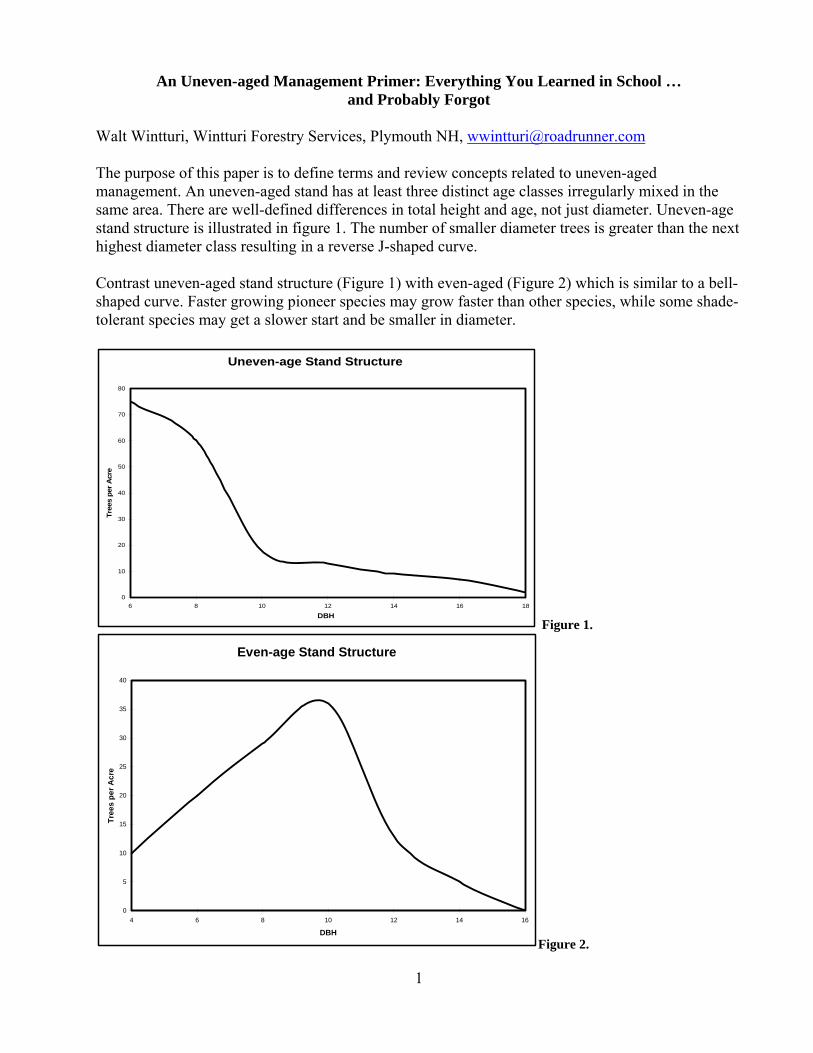
Walt Wintturi, Wintturi Forestry Services, Plymouth NH, wwintturi@roadrunner.com The purpose of this paper is to define terms and review concepts related to uneven-aged management. An uneven-aged stand has at least three distinct age classes irregularly mixed in the same area. There are well-defined differences in total height and age, not just diameter. Uneven-age stand structure is illustrated in figure 1. The number of smaller diameter trees is greater than the next highest diameter class resulting in a reverse J-shaped curve. Contrast uneven-aged stand structure (Figure 1) with even-aged (Figure 2) which is similar to a bell-shaped curve. Faster growing pioneer species may grow faster than other species, while some shade-tolerant species may get a slower start and be smaller in diameter.

Uneven-age Stand Structure

0

10

20

30

40

50

60

70

80

6 8 10 12 14 16 18

DBH

Tre

es

per

Acr

e

Figure 1.

Even-age Stand Structure

0

5

10

15

20

25

30

35

40

4 6 8 10 12 14 16

DBH

Tre

es

pe

r A

cre

Figure 2.

2

Figures 3 and 4 compare stand height against time and trees per acre versus time for even- and uneven-aged stands. Uneven-aged stand height remains relatively constant over time while even-aged stands start at the seedling height until they mature and reach the same height as uneven-aged stands. Even-aged stands start out with thousands of stems per acre—a number that diminishes as the stand matures.

Figure 3.

Figure 4.

3

Does a stand need to be an uneven-aged stand now in order to manage it under the uneven-aged system? No. If the forester or landowner decides that the objective of stand management is to manage it uneven-aged, then a prescription may be developed to initiate an uneven-aged structure. There are four reasons for managing stands through the uneven-aged system: 1) Stands were inherited and too many young trees would be cut if the stand were replaced by

clearcutting. 2) Aesthetic considerations. The management objective requires that the stand always contains

some large trees. 3) To develop or maintain winter cover for wildlife. 4) The habitat type (soil) is bested suited for growing shade-tolerant species, i.e. enriched, sugar

maple, beech fine till, softwood wet or dry pan. How large does a stand have to be to be considered a stand? How small an area do you want to keep stand records for? It’s the forester’s decision to make. For large ownerships usually ten acres is the smallest stand size, anything smaller than this is an inclusion. Uneven-aged stands: small irregular, even-aged groups. The groups are intermixed, not clearly separated. They are treated as uneven-aged from an organizational stand point. Selection system is the term applied to the silvicultural program aimed at developing or maintaining an uneven-aged stand. It includes periodic harvesting to start a new regeneration age class. Mature trees are removed as individuals or small groups at relatively short intervals—12 to 15 years. The time between intervals depends on growth rates, stand condition, and the size (value) of the desired harvest. It is well-suited to the regeneration of shade-tolerant species such as sugar maple, beech, hemlock, red spruce and balsam fir. Q Factor Q-factor is a measure that expresses stand structure. It is the diameter distribution diminution quotient. For example if there are 12 trees per acre in the 10-inch class and 9 trees per acre in the 12-inch class, then the q-factor is 12/9 = 1.3. The following table 5 illustrates another example of the calculation of q-factor. In this example the average q for the stand is 1.4. Stand Q Calculation

DBH Class Trees/acre Q4 110.1 6 56.6 1.98 22.9 2.510 12.0 1.912 10.2 1.214 5.1 2.016 5.6 0.918 4.0 1.420 3.2 1.222 1.9 1.724 0.8 2.226 1.0 0.828 0.8 0.328+ 2.3 0.3 18.3 18.3/13=1.4 Stand Q

4

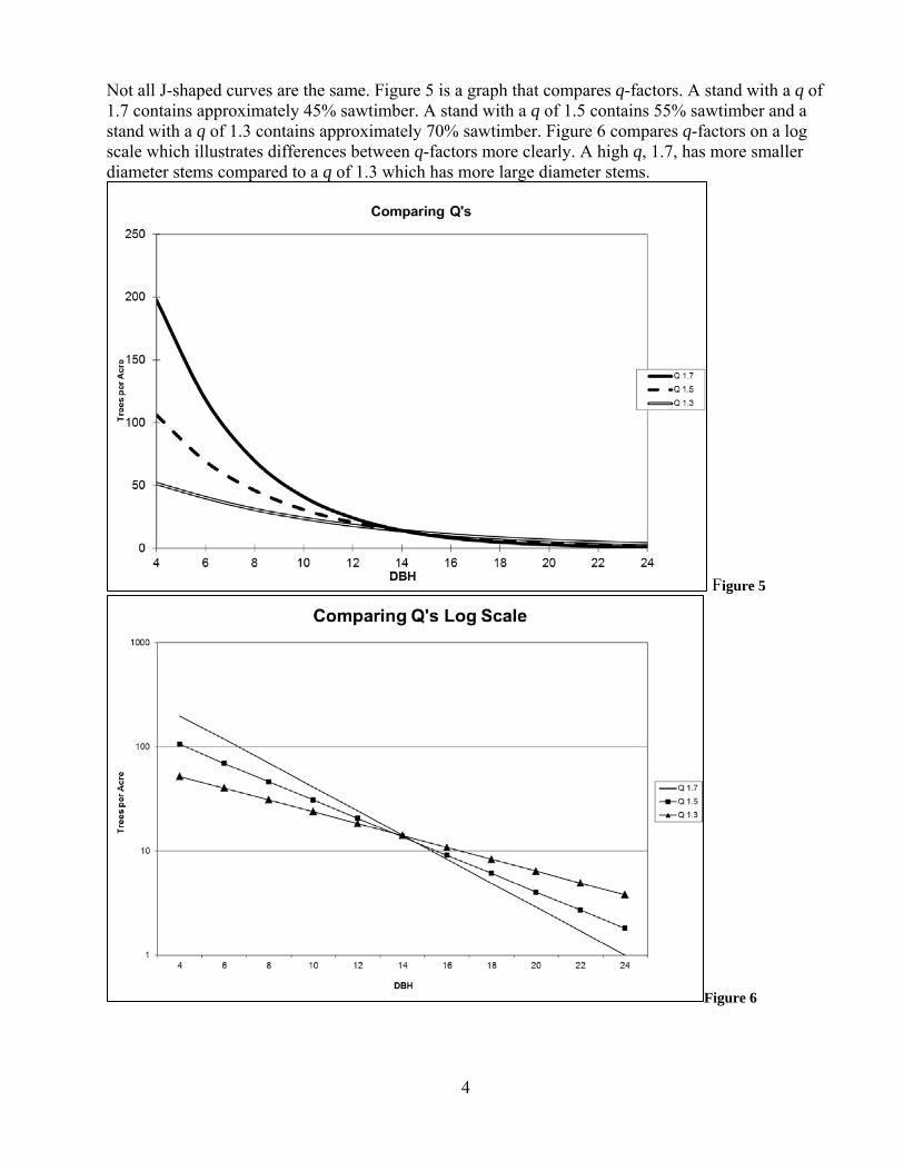
Not all J-shaped curves are the same. Figure 5 is a graph that compares q-factors. A stand with a q of 1.7 contains approximately 45% sawtimber. A stand with a q of 1.5 contains 55% sawtimber and a stand with a q of 1.3 contains approximately 70% sawtimber. Figure 6 compares q-factors on a log scale which illustrates differences between q-factors more clearly. A high q, 1.7, has more smaller diameter stems compared to a q of 1.3 which has more large diameter stems.

Figure 5

Figure 6

5

To choose a structural goal, consider the existing q of the stand, rates of growth, stand basal area, the size to which the largest trees are to be grown, and species. Choose a q the same or slightly lower than the existing q. Keep in mind that q-factors are mathematical not biological. The q is simply a guide. Be flexible. An inventory of the stand should be made before marking to gather the information to determine the stand q and from that determine where the surpluses and deficits are by diameter class. Need to determine distribution of diameter classes by basal area. The cut is made on the basis of a comparison between actual distribution to what is assumed to be balanced. Selection Method There are two prescriptions used to regenerate uneven-aged stands: 1) individual or single tree selection and 2) group selection. Individual tree selection promotes the development of even-aged groups of trees in very small, scattered openings. The species regenerated and perpetuated are very shade-tolerant—sugar maple, beech, hemlock, red spruce and balsam fir. Openings need to be continually enlarged to perpetuate young tree growth. Group selection seems to be a more feasible way to manage uneven-aged stands. Groups are two times the height of mature trees (For example, when trees are 75 feet tall, the group opening should be 150 feet in diameter, i.e. 2 X 75 feet = 150 feet). This may result in the regeneration of some shade-intolerant and intermediate-tolerant species—paper birch, white ash and yellow birch. A third selection system prescription is the improvement cut. This is applied to poletimber stands to improve residual tree quality by removing unacceptable growing stock and lower quality overstory stems. Marking Priority 1) High risk trees 2) Undesirable growing stock 3) Trees greater than the maximum diameter established for the stand 4) Slow growing trees 5) Undesirable species 6) Trees whose removal improves residual tree spacing Summary Silviculture is local. Develop an understanding of the tree responses on the habitat type (soils) the stand is growing on. The q-factor selected and the maximum tree size to grow is determined by the site. Diameter distribution is determined by the biology (ecology) of the forest and purposes of

management and not by mathematics. No reason to have a balanced stand. Work with what you have. With any approach to uneven-aged management, it is crucial to sustained yield to keep cutting

openings in stands for the recruitment of new regeneration. The selection system is complex requiring sophisticated prescriptions. Prescriptions take time—

three to four times more time.

6

Ecology of Uneven-aged Management

Thomas D. Lee, Associate Professor of Forest Ecology, University of New Hampshire, 172 Spaulding Life Sciences, Durham, NH 03824, (603) 862-3791, tom.lee@unh.edu Introduction One could easily write a book about the ecology of uneven-aged management, so we will focus here on just three rather specific topics. First, we will ask how uneven-aged management compares to natural disturbance regimes. Next, we will examine the impact of uneven-aged management on the physical environment of the forest, particularly on levels of sunlight and soil nutrients. Finally, we will ask what effects these physical changes have on understory vegetation, including tree regeneration and herb abundance. How does uneven-aged management compare to natural disturbance regimes? In recent years, there has been much interest in the relationship between silvicultural systems and natural disturbances. Some have suggested that when silviculture reflects the natural disturbance regime of a region, forest structure and tree species composition will most closely resemble that of ‘natural’ forests of that region, and the plants, animals, and microbes best adapted to this type of forest will be sustained over the long term. Even if one does not subscribe to this view—and there is considerable disagreement on this issue—a comparison of natural disturbance and silviculture may improve our understanding of how management influences forest structure.

Due to modification of the present landscape by humans, it is difficult to know precisely what natural disturbance regimes would prevail in New Hampshire today. We can get an idea of disturbance regimes prior to European settlement from the natural vegetation that covered the land at that time. Pre-settlement land surveyors often relied on ‘witness trees’ to mark corners, and survey records have allowed ecologists to crudely map forest composition as it was before land clearing began. Such maps suggest three broad forest types in pre-settlement New Hampshire (Figure 1). South of the White Mountains and east of the western uplands, pine-oak forest predominated. In the western uplands and in the valleys of the White Mountains, hardwood forest, dominated by American beech, was most abundant. Spruce and spruce-hardwood forest dominated at the higher elevations and north of the White Mountains.

What do these patterns suggest about disturbance regime? As oak and pine are not shade-tolerant, their abundance in the southeast suggests that natural disturbances in this region—evidence suggests hurricanes and wildfires—often created large canopy openings up to many acres in size. To the north and west, dominance of beech and spruce infers that the most common gaps were small (less than an acre), resulting from the death of one or a few canopy trees. Such gaps were likely caused by insects,

PINE-OAK

SPRUCE -HARDWOODS

BEECH -HARDWOODS

PINE-OAK

Figure 1. Map of New Hampshire showing approximate distribution of forest types in pre-settlement times, as indicated by early land surveys. (Map re-drawn from Cogbill et al. 2002.) Pine-oak region probably experienced more wildfire and hurricane damage; beech-hardwoods probably experienced smaller canopy gaps caused by insects, disease, wind.

7

disease, or wind. It is important to note that these gap sizes are only suggested as “typical” of these regions; certainly there were large areas of fire and wind damage in the northern hardwoods and there were areas that escaped such catastrophe in the pine-oak realm. (There are no absolutes in the natural world!) A mix of small gaps and larger catastrophic disturbances was probably typical of lowland spruce-fir stands. Recent research shows that, at elevations over 3,000 feet, chronic wind stress causes gaps to expand over time, eventually forming patches of disturbance many acres in size.

Our still incomplete knowledge of natural disturbance in New Hampshire suggests that uneven-aged management, particularly selective cutting and small group selection, most closely corresponds to disturbance regimes experienced by pre-settlement northern hardwoods and spruce-hardwoods, and perhaps some portions of the oak-pine region. In contrast, the larger disturbances of the oak-pine forest (and perhaps in parts of the lowland spruce-fir forest) created patches of even-aged timber similar to that generated by even-aged management and large group selection. Of course, it is important to remember that similar-sized openings created by cutting and natural causes differ in other important ways. Natural gaps lack stumps and skidder ruts but have more coarse woody debris than openings caused by logging. Both kinds of openings, however, change the physical environment of the forest, as discussed below. How canopy openings affect sunlight and soil nutrients Canopy openings increase levels of sunlight on the forest floor beneath them. However, in New Hampshire (in fact, in all forests north of the tropics), sunlight is never evenly distributed over the ground below an opening, because at mid-day the sun always shines out of the southern sky. Direct sunlight only illuminates the north-central portion of the opening, while the remainder is shaded by the adjacent forest, receiving only diffuse (reflected) light (Figure 2). Generally, the larger the opening, the more light reaches the forest floor. In small canopy gaps, direct sunlight might never reach the ground, ending up illuminating only the understory of the closed canopy forest north of the gap. Moreover, because small gaps are rapidly filled in by the growth of branches from adjacent canopy trees, they tend to exist for just a few years. Larger openings, in contrast, are gradually filled by the growth of new seedlings and advanced regeneration from within the gap itself, and remain open longer.

Looking at an entire stand (rather than an individual canopy gap), the quantity and distribution of light received on the forest floor is likely to be affected by the silvicultural system used. Single tree selection results in many small, short-lived openings. As these openings are regularly distributed and not too far apart, diffuse light prevents most of the forest floor from being densely shaded. In contrast, group selection results in fewer, larger gaps that last longer, have more direct sunlight

N

DIRECTSUNLIGHT

DIFFUSE DIFFUSE

Figure 2. In the temperate zone, direct sunlight reaches the ground only in the north-central part of a canopy gap and under the closed canopy just north of the gap. The southern, eastern, and western parts of the gap receive more light than the adjacent forest, but this light is mainly diffuse (reflected) and less intense than direct sunlight.

8

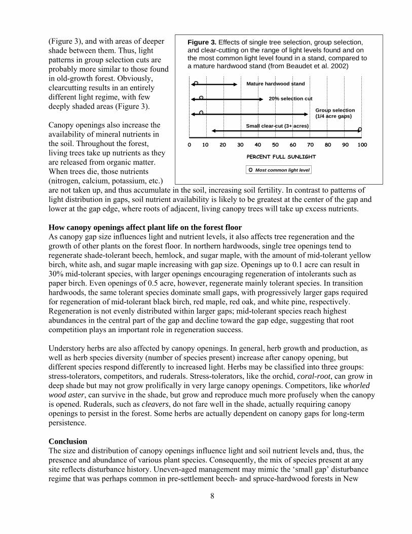
(Figure 3), and with areas of deeper shade between them. Thus, light patterns in group selection cuts are probably more similar to those found in old-growth forest. Obviously, clearcutting results in an entirely different light regime, with few deeply shaded areas (Figure 3).

Canopy openings also increase the availability of mineral nutrients in the soil. Throughout the forest, living trees take up nutrients as they are released from organic matter. When trees die, those nutrients (nitrogen, calcium, potassium, etc.) are not taken up, and thus accumulate in the soil, increasing soil fertility. In contrast to patterns of light distribution in gaps, soil nutrient availability is likely to be greatest at the center of the gap and lower at the gap edge, where roots of adjacent, living canopy trees will take up excess nutrients. How canopy openings affect plant life on the forest floor As canopy gap size influences light and nutrient levels, it also affects tree regeneration and the growth of other plants on the forest floor. In northern hardwoods, single tree openings tend to regenerate shade-tolerant beech, hemlock, and sugar maple, with the amount of mid-tolerant yellow birch, white ash, and sugar maple increasing with gap size. Openings up to 0.1 acre can result in 30% mid-tolerant species, with larger openings encouraging regeneration of intolerants such as paper birch. Even openings of 0.5 acre, however, regenerate mainly tolerant species. In transition hardwoods, the same tolerant species dominate small gaps, with progressively larger gaps required for regeneration of mid-tolerant black birch, red maple, red oak, and white pine, respectively. Regeneration is not evenly distributed within larger gaps; mid-tolerant species reach highest abundances in the central part of the gap and decline toward the gap edge, suggesting that root competition plays an important role in regeneration success.

Understory herbs are also affected by canopy openings. In general, herb growth and production, as well as herb species diversity (number of species present) increase after canopy opening, but different species respond differently to increased light. Herbs may be classified into three groups: stress-tolerators, competitors, and ruderals. Stress-tolerators, like the orchid, coral-root, can grow in deep shade but may not grow prolifically in very large canopy openings. Competitors, like whorled wood aster, can survive in the shade, but grow and reproduce much more profusely when the canopy is opened. Ruderals, such as cleavers, do not fare well in the shade, actually requiring canopy openings to persist in the forest. Some herbs are actually dependent on canopy gaps for long-term persistence. Conclusion The size and distribution of canopy openings influence light and soil nutrient levels and, thus, the presence and abundance of various plant species. Consequently, the mix of species present at any site reflects disturbance history. Uneven-aged management may mimic the ‘small gap’ disturbance regime that was perhaps common in pre-settlement beech- and spruce-hardwood forests in New

Figure 3. Effects of single tree selection, group selection, and clear-cutting on the range of light levels found and on the most common light level found in a stand, compared to a mature hardwood stand (from Beaudet et al. 2002)

0 10 20 30 40 50 60 70 80 90 100

PERCENT FULL SUNLIGHT

Mature hardwood stand

20% selection cut

Group selection (1/4 acre gaps)

Small clear-cut (3+ acres)

Most common light level

9

Hampshire, and is likely to perpetuate an assemblage of plant species typical of those types. Uneven-aged management may not mimic the larger disturbances that typified the pine-oak region. It is important to note, however, that no one really knows exactly what our pre-settlement forests looked like. Large disturbances and even-aged stands certainly occurred in northern hardwoods, and some of the pine-oak region may have escaped frequent extensive disturbance. In the end, choice of a silvicultural system depends on a set of specific landowner objectives, and these may not or may not include precise duplication of pre-settlement stand structure. References Natural Disturbance Cogbill, C.V., J. Burk, and G. Motzkin. 2002. Journal of Biogeography 29:1279. Lorimer, C.G. and A.S. White. 2003. Forest Ecology & Management 185:41. Roe, J.H. and A. Ruesink. Natural dynamics silviculture. The Nature Conservancy. Seymour, R.S., A.S. White, P.G. deMaynadier. 2002. Forest Ecology & Management 155:357. Worrall, J. J., T. D. Lee and T. C. Harrington. 2005. Journal of Ecology 93:178. Light Distribution Beaudet, M., C. Messier, and C.D. Canham. 2002. Forest Ecology and Management 165:235. Nyland, R.D. 1996. Silviculture: principles and applications. McGraw-Hill, New York. 633 pp. Plant Response Halpern, C.B., D. McKenzie, S.A. Evans, and D.A. Maguire. 2005. Ecological Appl. 15:175. Hibbs, D.E. 1982. Canadian Journal of Forest Research 12:522. Leak, W.B. and Filip, S.M. 1975. USDA Forest Service Research Paper NE-322. McClure, J.W. and T.D. Lee. 1993. Canadian Journal of Forest Research 23:1347. Scheller, R.M. and D.J. Mladenoff. 2002. Ecological Applications 12:1329.

10

Uneven-Aged Management and Wildlife Habitats—What Do We Know?

Mariko Yamasaki, USDA Forest Service, Northern Research Station, 271 Mast Road, Durham, NH 03824, myamasaki@fs.fed.us Wildlife habitats are dynamic by nature; and created or modified by natural or anthropogenic processes (e.g., glaciation, disturbance regime, succession, and forest management) and time across landscapes. Silvicultural approaches provide different configurations of habitat elements depending on the scale of application and size of openings used. Land managers have an opportunity to manipulate regional landscapes, local forest tracts, and individual stands to meet both wildlife habitat needs recognized in state comprehensive wildlife plans (NH Fish and Game Department 2005) and produce a variety of quality forest products through active management; as well as executing no-management options. This paper concentrates on habitats elements created through silvicultural practices associated with New England forest types. Even-aged and uneven-aged management are two silvicultural strategies utilized in New England. To address the relative values of habitats provided through silvicultural manipulations, I need to address the habitat elements provided in both strategies. Uneven-aged management encompasses two general practices—single-tree selection and group/patch selection (Leak et al. 1987). Even-aged management is implemented either through clearcutting or shelterwood practices. Three basic elements determine the relative habitat importance of any of these silvicultural practices: 1) opening size and frequency of occurrence; 2) species composition of regeneration and subsequent stands; and 3) structural habitat characteristics presented or eliminated through management. Even-aged management practices create larger openings and more substantial early successional habitat than either single-tree or group/patch selection practices (DeGraaf and Yamasaki 2003). Single-tree selection offers more immediate closed canopy habitat than either group/patch selection or even-aged practices. As such there are usually tolerant midstory and understory layers present. Opening size influences plant species composition in managed stands as well. The proportion of intolerant tree regeneration (e.g., aspen and paper birch) increases with opening size (Leak et al. 1987). Tolerant species regeneration (e.g., beech, sugar maple, hemlock, and red spruce) is favored in uneven-aged management practices. Intermediate species (e.g., yellow birch, red maple, white ash, and white pine) as well as tolerant species regenerate well in group/patch selection practices. Intolerant tree species and soft mast species (e.g., raspberry, blackberry, strawberry, blueberry, pin cherry) flourish in sun-drenched larger openings along with intermediate and tolerant species. Larger group selection openings (> 0.5 acre) also allow for intolerant species regeneration. Holmes and Robinson (1981) documented avian foraging specializations on various northern hardwood species and the insects found upon them. The structural habitat characteristics found in various silvicultural strategies involve canopy conditions, particular tree types (e.g., perch types, cavity trees, coarse woody debris, and mast), and vertical structure conditions (Table 1). Closed to partial canopy conditions range from tree-sized and small gaps averaging 0.5 acre using single-tree and group/patch selection. Even-aged management creates considerably larger canopy openings that eventually close in time. Many bird species utilize very different canopy conditions during the year (e.g., breeding versus pre-migration habitat), thus

11

reinforcing the importance of providing a range of habitat conditions across managed landscapes. Overstory inclusions can be a part of any silvicultural strategy. High and low exposed perches can be found in group/patch selection and even-aged management practices because of the relatively ephemeral openness around perch sites that are conducive to hunting raptors and flycatchers; as well as being song perches for various passerines. Large cavity trees, important to cavity-dwelling woodpeckers (Gunn and Hagan 2000) and other wildlife species can be present in any silvicultural strategy provided that such trees are part of stand prescriptions at densities recommended in Tubbs et al. (1987). The presence of large coarse woody debris in managed stands depends on the stand prescription: growing trees large enough and allowing some to die, decay, and fall over in the stand; as well as distributing no-cut or minimally-cut buffers throughout the managed landscape. Prescriptions that minimize stand mortality through frequent thinnings and harvests will probably have a minimal large coarse woody debris component over time. Hard mast (e.g., nut bearing species) can be found in no-management and single-tree management strategies. Regenerating oaks using group/patch selection and shelterwood practices requires time to produce a substantial nut crop. Soft mast occurs where substantial sunlight gets to the forest floor for a few years. Larger group/patch selection practices and even-aged management practices offer the best opportunities to produce a variety of soft mast species but only until the overstory begins to close. Tolerant midstory layers occur in no-management and single-tree selection practices. Such layers develop in time in group/patch selection and even-aged management practices. Forage-rich shrub and ground cover layers are ephemeral habitat elements in group/patch selection and even-aged management practices. The insect loads available in such treatments for avian and bat foraging are greater; and the plant diversity available as forage for large herbivores is more nutritious than in shade-grown conditions (Hughes and Fahey 1991). Cutting effects on redback salamander habitat are temporary (DeGraaf and Yamasaki 2002); small gaps are fully reoccupied sooner than large cuts. Movement opportunities for mole salamander and frog species between temporary wetlands and adjacent forested uplands need to be maintained. Many reptile species use basking sites in open sunny sites; as well as lay eggs in open, sandy, gravelly nest sites. Birds tend to be the most responsive taxa to vegetative structure. DeGraaf (1991) described the highly ephemeral nature of avian breeding response in newly regenerating hardwood stands, which were very different from mature stands. Mature, overmature, and uneven-aged stands of northern hardwoods produced similar breeding bird communities (DeGraaf 1991). Costello et al. (2000) found that group selection cuts averaging 0.5 acre provided breeding habitat for some but not all of the species found using larger clearcuts averaging 20 acres, as well as mature hardwoods. Larger openings may be important pre-migration foraging areas for neotropical migrants (C. Kaufman, pers. comm.). Tree-nesting raptor species often place their nests in close proximity to small gaps, openings, and trails. Management practices that maintain large snags and other wildlife trees throughout stands benefit a wide range of cavity-dwelling species. Small mammals are mostly unaffected by silvicultural practice except for meadow voles and meadow jumping mice (Yamasaki, unpubl. data). Bats fly and forage in a variety of forest opening sizes (Krusic et al. 1996). Large herbivores can influence forest regeneration at higher population

12

levels; and require a variety of opening sizes, brushy impediments, higher forage loads and cooperative herd management strategies to successfully regenerate forest stands. Single-tree selection used across extensive landscapes tends to: 1) limit horizontal diversity; 2) decrease the amount and distribution of quality browse; and 3) restrict the early and mid-successional foraging substrates used by both herbivores and insectivores alike. Group/patch selection provides habitat conditions between single-tree selection and even-aged approaches. On average, even-aged management provides more habitat opportunities for a wider variety of wildlife species than uneven-aged management (DeGraaf et al. 1992). Thus, it is important to maintain both even-aged and uneven-aged management practices in the tool bags of practicing foresters and wildlife biologists. Literature Cited Costello, C.A., M. Yamasaki, P.J. Pekins, W.B. Leak, and C.D. Neefus. 2000. Songbird response to group selection harvests and clearcuts in a New Hampshire northern hardwood forest. For. Ecol. Manage. 127: 41-54. DeGraaf, R.M. 1991. Breeding bird assemblages in managed northern hardwood forests in New England. Pages 154-171. In: Rodiek, J.E. and E.G. Bolen (editors). Wildlife and habitats in managed landscapes. Washington, D.C.: Island Press. DeGraaf, R.M., M. Yamasaki, W.B. Leak, and J. Lanier. 1992. New England Wildlife: Management of Forested Habitats. USDA Forest Service, Gen. Tech. Rep. NE-144. DeGraaf, R.M. and M. Yamasaki. 2002. Effects of edge contrast on redback salamander distribution in even-aged northern hardwoods. For. Sci. 48: 351-364. DeGraaf, R.M. and M. Yamasaki. 2003. Options for managing early-successional forest and shrubland bird habitats in the northeastern United States. For. Ecol. Manage. 185: 179-191. DeGraaf, R.M., M. Yamasaki, W.B. Leak, and A.M. Lester. 2005. Landowner’s Guide to Wildlife Habitat: Forest Management for the New England Region. Lebanon, NH: University Press of New England. 128 p. Gunn, J.S. and J.M. Hagan III. 2000. Woodpecker abundance and tree use in uneven-aged managed, and unmanaged, forest in northern Maine. For. Ecol. Manage. 126: 1-12. Holmes, R.T. and S.K. Robinson. 1981. Tree species preferences of foraging insectivorous birds in a northern hardwoods forest. Oecologia. 48: 31-35. Hughes, J.W. and T.J. Fahey. 1991. Availability, quality, and selection of browse by white-tailed deer after clearcutting. For. Sci. 37: 261-270. Krusic, R.A., M. Yamasaki, C.D. Neefus, and P.J. Pekins. 1996. Bat habitat use in White Mountain National Forest. J. Wildl. Manage. 60: 625-631. Leak, W.B., D.S. Solomon, and P.S. DeBald. 1987. Silvicultural guide for northern hardwood types in the northeast (revised). USDA Forest Service, Res. Pap. NE-603. New Hampshire Fish and Game Department. 2005. NH Wildlife Action Plan. Concord. Tubbs, C.H., R.M. DeGraaf, M. Yamasaki, and W.M. Healy. 1987. Guide to wildlife tree management in New England northern hardwoods. USDA Forest Service, Gen. Tech. Rep. NE-118.

13

Table 1. Characteristic habitat elements provided through management strategies (adapted from DeGraaf et al. 2005).

No Management Uneven-aged Management Even-aged Management

Element Single-tree Group/Patch Canopy Characteristics

Closed canopy Tree-sized gaps Tree-sized gaps Closes in time Partial canopy Small gaps Open canopy Large gapsa Overstory inclusions

Presentb X X X

Perches, Cavity Trees, Coarse Woody Debris, and Mast

High perches X X Low perches X X Large cavity trees

Abundant Xc Xc Xc

Coarse woody debris

Abundant Minimald Xd Xd

Hard mast X X NIe NI Soft mast X X Vertical Structure

Midstory X X NI NI Shrub layer X X Ground cover layer

X X

a When first cut. b Routinely occurring in the management strategy. c Stands marked to provide a minimum of 3-5 large live cavity trees per acre in patches and leave strips in addition to all the other uncut large dead trees in the stand. Large cavity trees near water are important structural features and can be maintained in riparian buffers. d Any timber management activity can reduce coarse woody debris recruitment in stands over time. Leaving large cull trees and particularly hollow trees, can provide such shelter features in managed stands when they fall. e NI = Not immediately occurring in the management strategy.

14

The Reverse-J and Beyond: Developing Practical, Effective Marking Guides

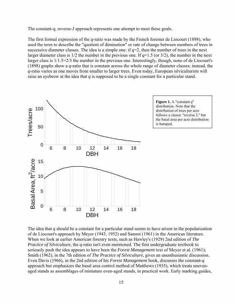
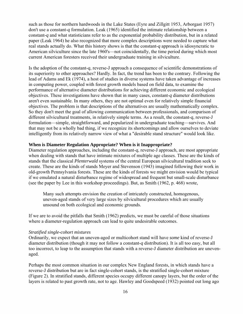
Mark J. Ducey, Professor of Forest Biometrics, University of New Hampshire, 215 James Hall, Durham, NH 03824, mjducey@cisunix.unh.edu Introduction The reverse-J shaped curve, and specific versions of it, have become synonymous with uneven-aged silviculture in American practice. It has its role, but there are other alternatives. It is important to understand the goals of silviculture and the biological assumptions behind the use of a reverse-J curves, before using them to develop practical marking guides. At the same time, it is important for practical guides to respect the real limits foresters encounter in their operational environment. These limits include the quality of inventory information, and the ability for (or even wisdom of!) sticking rigidly to precise numerical guides in complex forest stands. Here, we'll look at a brief history of the reverse-J, and the goals and assumptions behind diameter regulation of uneven-aged stands. These assumptions will lead us to spell out some situations in which a reverse-J, diameter regulation approach is probably not a good choice. We'll take a look at the three parameters (basal area, maximum tree diameter, and q-ratio) that are most often used to describe a reverse-J target structure. Some simplification and flexibility is useful when putting the reverse-J into practice, and we'll conclude with a simplified system for developing marking guidelines. History and Goals Ask most foresters how to do uneven-aged management, and you're likely to get an answer that includes the application of a reverse-J shaped curve, described by a constant q-ratio, to decide how many trees to cut and how many to retain within each diameter class. An example is shown in Figure 1. Note that while the distribution of trees per acre is reverse-J shaped, the distribution of basal area per acre is humped. Like the use of site index to describe site quality, the constant-q, reverse-J approach has become so popular that it can be difficult to remember there are other alternatives. But the constant-q reverse-J shape is a relatively recent development in silvicultural practice—a development that is younger, anyway, than many of the trees we are harvesting—and one that is especially, though not exclusively, associated with American approaches to uneven-aged management. The use of the reverse-J curve is a special case of diameter regulation, the idea that we can sustain production in an uneven-aged stand by maintaining a consistent residual distribution of sizes (and, we hope, ages) of trees after each harvest entry. In this sense, the goals of diameter regulation are the same as those of volume regulation in a large, uneven-aged landscape compose of even-aged stands (Meyer et al. 1961). A successful approach to diameter regulation would achieve the following goals: Regulate the harvest, to ensure that overcutting does not occur. Ensure sustainability, by providing for adequate regeneration and vigorous growth of the residual

trees. Prescribe stand structures that lead to desirable outcomes, including stability in site protection,

positive habitat values, economic productivity, and aesthetically attractive stands. Allow communication between professionals, and comparison of different silvicultural treatments,

in relatively simple terms. Provide a repeatable basis for experimental design.

15

The constant-q, reverse-J approach represents one attempt to meet these goals. The first formal expression of the q-ratio was made by the French forester de Liocourt (1898), who used the term to describe the "quotient of diminution" or rate of change between numbers of trees in successive diameter classes. The idea is a simple one: if q=2, then the number of trees in the next larger diameter class is 1/2 the number in the previous one. If q=1.5 (or 3/2), the number in the next larger class is 1/1.5=2/3 the number in the previous one. Interestingly, though, none of de Liocourt's (1898) graphs show a q-ratio that is constant across the whole range of diameter classes; instead, the q-ratio varies as one moves from smaller to larger trees. Even today, European silviculturists will raise an eyebrow at the idea that q is supposed to be a single constant for a particular stand.

The idea that q should be a constant for a particular stand seems to have arisen in the popularization of de Liocourt's approach by Meyer (1943, 1952) and Sammi (1961) in the American literature. When we look at earlier American forestry texts, such as Hawley's (1929) 2nd edition of The Practice of Silviculture, the q-ratio isn't even mentioned. The first undergraduate textbook to seriously push the idea appears to have been the Forest Management text of Meyer et al. (1961); Smith (1962), in the 7th edition of The Practice of Silviculture, gives an unenthusiastic discussion. Even Davis (1966), in the 2nd edition of his Forest Management book, discusses the constant-q approach but emphasizes the basal area control method of Matthews (1935), which treats uneven-aged stands as assemblages of miniature even-aged stands, in practical work. Early marking guides,

6 8 10 12 14 16 180

50

100

DBH

Tre

es/a

cre

6 8 10 12 14 16 180

5

10

15

DBH

Bas

al A

rea,

ft2/a

cre

Figure 1. A "constant q" distribution. Note that the distribution of trees per acre follows a classic "reverse J," but the basal area per acre distribution is humped.

16

such as those for northern hardwoods in the Lake States (Eyre and Zillgitt 1953, Arborgast 1957) don't use a constant-q formulation. Leak (1965) identified the intimate relationship between a constant-q and what statisticians refer to as the exponential probability distribution, but in a related paper (Leak 1964) he also recognized that more complex descriptions were needed to capture what real stands actually do. What this history shows is that the constant-q approach is idiosyncratic to American silviculture since the late 1960's—not coincidentally, the time period during which most current American foresters received their undergraduate training in silviculture. Is the adoption of the constant-q, reverse-J approach a consequence of scientific demonstrations of its superiority to other approaches? Hardly. In fact, the trend has been to the contrary. Following the lead of Adams and Ek (1974), a host of studies in diverse systems have taken advantage of increases in computing power, coupled with forest growth models based on field data, to examine the performance of alternative diameter distributions for achieving different economic and ecological objectives. These investigations have shown that in many cases, constant-q diameter distributions aren't even sustainable. In many others, they are not optimal even for relatively simple financial objectives. The problem is that descriptions of the alternatives are usually mathematically complex. So they don't meet the goal of allowing communication between professionals, and comparison of different silvicultural treatments, in relatively simple terms. As a result, the constant-q, reverse-J formulation—simple, straightforward, and popularized in undergraduate teaching—survives. And that may not be a wholly bad thing, if we recognize its shortcomings and allow ourselves to deviate intelligently from its relatively narrow view of what a "desirable stand structure" would look like. When is Diameter Regulation Appropriate? When is it Inappropriate? Diameter regulation approaches, including the constant-q, reverse-J approach, are most appropriate when dealing with stands that have intimate mixtures of multiple age classes. These are the kinds of stands that the classical Plenterwald systems of the central European silvicultural tradition seek to create. These are the kinds of stands Meyer and Stevenson (1943) imagined following their work in old-growth Pennsylvania forests. These are the kinds of forests we might envision would be typical if we emulated a natural disturbance regime of widespread and frequent but small-scale disturbance (see the paper by Lee in this workshop proceedings). But, as Smith (1962, p. 468) wrote,

Many such attempts envision the creation of intricately constructed, homogenous, uneven-aged stands of very large sizes by silvicultural procedures which are usually unsound on both ecological and economic grounds.

If we are to avoid the pitfalls that Smith (1962) predicts, we must be careful of those situations where a diameter-regulation approach can lead to quite undesirable outcomes. Stratified single-cohort mixtures Ordinarily, we expect that an uneven-aged or multicohort stand will have some kind of reverse-J diameter distribution (though it may not follow a constant-q distribution). It is all too easy, but all too incorrect, to leap to the assumption that stands with a reverse-J diameter distribution are uneven-aged. Perhaps the most common situation in our complex New England forests, in which stands have a reverse-J distribution but are in fact single-cohort stands, is the stratified single-cohort mixture (Figure 2). In stratified stands, different species occupy different canopy layers, but the order of the layers is related to past growth rate, not to age. Hawley and Goodspeed (1932) pointed out long ago

17

that mixed-species, even-aged hardwood stands could have a reverse-J distribution. Further work by D.M. Smith and his students, notably Oliver (1978, 1981), tied this recurring phenomenon to more general processes from the ecological literature (Egler 1954). The challenge is particularly acute in New England because our stands are among the most complex (in terms of species composition) outside the tropics. Furthermore, many of our stands are essentially single-cohort stands because of natural disturbance regimes (especially in areas dominated by oak and pine; see the chapter by Lee in this proceedings) or because of land-use history. Simply put, many of our stands do have reverse-J distributions but are not uneven-aged, and do not respond to silvicultural interventions the way uneven-aged stands would. The danger of misapplying diameter regulation methods to stands that are essentially even-aged is that of "high-grading by stages" (Smith 1992, p. 287). In stands where the lower strata are composed of shade-tolerant species like eastern hemlock, American beech, and red maple, trying to imitate single-tree selection preferentially removes the less-tolerant, faster-growing (and often more valuable) trees such as the pines, oaks, birches, and ash. The small gaps that are created are often captured fairly quickly by the lower-stratum trees; no regeneration occurs. (Where regeneration does occur, it often takes the form of beech suckers.) This is, indeed, the nightmare scenario for misapplication of selection management. On good sites, the lower stratum may be dominated by sugar maple. Simplification of a complex stratified mixture to a stand dominated by sugar maple may or may not be a bad thing, depending on the goals of management. Still, we should be cautious about assuming the stand at the end of this process will be uneven-aged. Conversion and transitional stands Perhaps we have an even-aged or single-cohort stand, and we would like to convert it to an uneven-aged stand. Or, perhaps we have inherited a mess from someone else's past "silviculture," and conversion to an uneven-aged condition seems appropriate. (A common enough form of such "messes" is a two-cohort stand. The older cohort is comprised of trees that were left behind after diameter-limit cutting or "commercial clearcutting" long ago; the younger cohort, often a heavy, mixed thicket, is comprised of the trees that became established in response to the cut.) Is a diameter-regulation approach useful in these cases? The conversion situation is particularly challenging. Kelty et al. (2003) provide a recent review that, while focused on southern and central New England, also summarizes the results of studies in northern New England. They concluded that patch selection might be the most straightforward approach to stand conversion. The chapter by Kelty in this proceedings provides further insights on this issue. In a nutshell, attempting to convert single-cohort stands using diameter regulation can lead to the same problems as managing them using diameter regulation out of ignorance. (The trees, unfortunately, have no central nervous system and cannot respect our intelligence or intentions.) These problems can include species conversion and simplification, selection against vigor within species, and the failure (even after multiple entries) to break the competitive hold of the predominant cohort. In inherited stands, a diameter regulation approach may be more appropriate, depending on stand condition. However, other priorities demand our attention in dealing with such stands. These priorities often fall under the broad category of rehabilitation: improving the species and grade mix of a depleted or degraded stand, breaking up the "thicket" so that smaller trees are free to grow, and allowing any remaining large, desirable trees to develop vigorous crowns and resilient, tapering stems before committing to significant regeneration cutting. Diameter regulation may be useful in

18

setting broad structural targets in the rehabilitation process, but the goal of rehabilitation must take precedence. Group and patch selection Is diameter regulation appropriate for group and patch selection methods? These methods do not seem to represent the kind of intricate, intimate mixtures that Meyer (1943) envisioned, or that Smith (1962) hedged against. And it is certainly true that one approach to constructing a reverse-J curve is to consider the uneven-aged stand as a patchwork of tiny even-aged stands (Matthews 1935). Having said that, for group and patch selection with patches of any recognizable size (say, 0.25 acre or more), there is a simpler alternative: area regulation. Cut the right number and area of patches at each entry, and the diameter distribution will follow. This approach is simple, it is robust to the sampling error that pre-marking cruises show, and it requires almost no cumbersome math. The paper by Kelty et al. (2003), and the chapters by Leak and by Kelty in this proceedings, give some useful guidance for formulating area regulation approaches in group selection. BDq: The Classical Approach You have made it through the caveats and warnings. Perhaps you have already decided that the ecology and management objectives of (at least some of) your stands are compatible with a diameter-regulation approach. Perhaps because of its (supposed) simplicity, the classical approach (reverse-J with a constant-q) seems like a good method. What is involved in putting this method into practice? Every diameter regulation approach requires three pieces of information to specify what the stand should look like just after harvest. These three pieces of information are the residual stocking (using some appropriate stand density measure), the maximum diameter that trees will be allowed to reach (whether by the forester, or by nature), and the shape of the diameter distribution. In what I will call the "classic approach," because it is the approach most often used by American foresters (Guldin 1996), the stocking measure is basal area per acre (B), the maximum diameter is some number in inches (D), and the shape of the diameter distribution is completely specified by a single value of q. Let's examine each of these pieces of information in turn. B, basal area (ft2/acre) to leave. There are many measures of stand density to choose from, and basal area certainly has its shortcomings, even in single-species stands (Zeide 2005). Basal area has little or no direct biological meaning. However, it is commonly used, and that facilitates communication. It is easily measured (just use a prism), and that can be a significant advantage in an age that prizes accountability. Finally, it is closely related to stand volume, and a primary motivation for diameter regulation is to serve as a stand-scale approximation to volume regulation. In principle, one might use the total basal area per acre of a stand. However, most foresters do not have the luxury of making decisions about very small trees, and not all have the patience to measure them. As a practical matter, then, the basal area used in diameter regulation is often specified as the basal area of trees above some minimum diameter. For example, the current northern hardwood silvicultural guide (Leak et al. 1987) specifies B in terms of trees in the 6-inch class and larger (i.e., trees from 5.0 inches DBH and up). Basal area may be the most critical part of BDq, because the residual basal area will have a very strong influence on how much (if any) desirable regeneration occurs, and how fast (or whether) the

19

residual stems will grow. A common error is setting the residual basal area too high. The resulting stand often looks good, but there simply isn’t enough growing space to get new trees in or to move the small trees along at a financially reasonable rate. An appropriate value of B is often a fairly low value (60 to 80 ft2/acre in some northern hardwood stands). It depends not only on biology, but also on the cutting cycle: set B too high and wait too long, and the stand will close up and stagnate; but set it too low and come back too soon, and there won’t be a merchantable cut. D, maximum diameter of trees to leave. Historically, the focus of selection management was financial productivity subject to other constraints (such as site protection), and choosing a value of D has a strong influence on measures of financial productivity such as internal rate of return (see the chapter by Howard in this proceedings). Setting D too low can mean forgoing the opportunity to produce large, high grade, extremely valuable trees. But setting it too high (especially when B is high enough that growth is not rapid) can mean waiting too long for financial returns. Valuable capital is left tied up on the stump, and an adequate rate of return cannot be achieved. Moreover, large trees may be subject to other damage (both natural, such as root rot, windthrow, frost cracks, or lightning; and human-caused, especially basal or root damage during harvesting). The other side of this coin is that D is also critical to achieving many of the structural and ecological goals of “nature-based silviculture.” To put it bluntly, if live trees are not grown to a large size, and if some of those large live trees are never harvested, there will never be large snags, large downed logs, and so on. It is easy to design a single-tree selection system that is financially attractive but achieves none of these structural or ecological goals. D plays a critical role here, and one that is often in opposition to its role in strictly financial criteria. q, “quotient of diminution” for the stand. We’ve already seen q described. The choice of q sets the shape of the diameter distribution. It’s worth remembering here what Meyer (1943) said the goal of all this diameter regulation was: “to secure and maintain an adequate balanced growing stock capable of producing a sustained annual or periodic yield.” The choice of q will certainly impact financial performance. A low value of q will concentrate the allocation of growing space on larger trees, so that the current rate of value production will be high. On the other hand, that also means a lot of valuable capital is tied up in the woods, so a very high rate of value production is needed to turn a reasonable interest rate...which is why many optimization studies have focused on high values of q, which leave relatively few large trees to grow. Other goals (vertical structure, large trees as habitat elements, and so on) will also be affected by the choice of q. The choice of q is not one we can make arbitrarily. Smith et al. (1997, pp. 376-377) heavily criticize Meyer (1952) for assuming, without verification, that stands with any “reasonable,” constant-q had arrived at a stable, self-sustaining state. There is an important trade-off in stand dynamics, between providing enough small trees to replace the larger trees that die or are harvested, and avoiding a stagnant thicket in the understory. The Classical Approach: Is It Practical? At first, the title of this section doesn’t even seem like a real question. Marking a stand to a q is a staple lab exercise in undergraduate silviculture courses. Plenty of stands around the world have been marked to a q, sometimes repeatedly, in demonstration or research forests. The standard procedure goes more or less like this. You inventory the stand, and then (either based on management objectives, or trying to fit a q-relationship to the inventory data) you calculate how

20

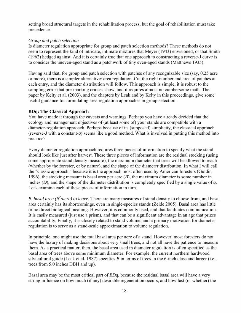
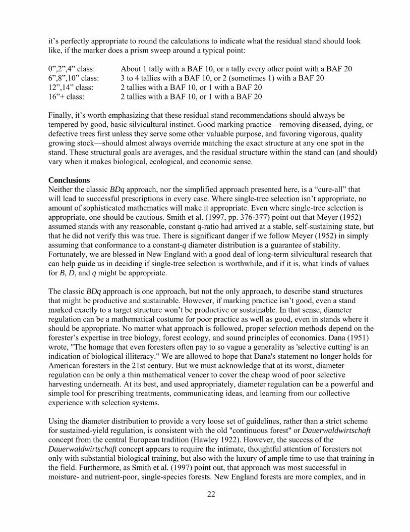
many trees per acre should be left in each diameter class. That calculation is tedious to do by hand, and almost universally hated. The excess is what you get to cut on this cutting cycle. Presumably, the residual trees will grow, and the next time you come back, there will be a similar amount of extra trees. The prescription stage of this process is illustrated in Figure 2. The standard procedure works very well, when the data about the initial stand conditions are very tight. That’s fairly common on research and demonstration forests, where a lot of effort is expended to be sure those conditions are well-known. It’s also easy enough to arrange in a tiny patch of woods that is used for a class exercise. But in a large stand, being managed under difficult financial and time constraints, inventory data simply isn’t usually very precise. That’s especially true when you zoom in on individual diameter classes. Typical inventory data—even when there are 15 to 25 prism points in a stand—may tell us the overall volume and basal area quite accurately, but that accuracy doesn’t usually carry down to an individual diameter class, which might only have a handful of tallied trees. Figure 3 illustrates the kind of problem that can arise. When the inventory data are inaccurate, the prescription will be inaccurate. Then, the residual stand won’t conform to the desired diameter distribution, despite our best intentions.

Figure 2. An idealized prescription situation. The target structure for the stand is given by the white bars. An inventory shows there are extra trees in each class (gray bars). Those are the trees to cut.

Figure 3. In real life, the cruise data are sample data, and can be very noisy. Each solid line is a realistic inventory result from this stand. Noise in the data translates directly into errors in the prescription.

21

One “solution” is to recognize that we probably won’t match a nice, smooth reverse-J curve exactly. If we use broader diameter classes—so that our inventory data for each class is less noisy—we can streamline the process, and focus on the big picture. More Practical Marking Guides To simplify the prescription process and the marking procedures, we’ll lump standard 2-inch diameter classes into larger “bins.” In principle, we could lump diameter classes any way we wanted to. For simplicity, and because it is familiar to many New England foresters, I’ve used the diameter classes in the Leak et al. (1987) northern hardwood guide. Also, instead of using trees per acre, we’ll use basal area per acre. That way, the markers can check themselves easily with a prism sweep to see if the trees that are not being marked have about the right diameter distribution. The main challenge in representing the “simple” constant-q structure for arbitrary diameter classes, is that calculating the amount of basal area to leave in grouped classes (and avoiding rounding error) would require some calculus. Fortunately, the results can be arranged in a set of tables that are easy to use. A set of these tables is in the Appendix to this section. The tables look like this: D=20” Diameter Class q 0, 2, 4 6, 8, 10 12, 14 16+ Total 6+ Total1.2 0.04 0.26 0.30 0.44 1.00 1.041.3 0.06 0.32 0.30 0.38 1.00 1.061.4 0.09 0.38 0.30 0.32 1.00 1.091.5 0.12 0.44 0.29 0.27 1.00 1.121.6 0.16 0.50 0.28 0.22 1.00 1.161.7 0.20 0.54 0.27 0.19 1.00 1.201.8 0.25 0.59 0.25 0.16 1.00 1.25 There are multiple tables, and you should use the table that corresponds to the value of D you would like for the stand: the maximum size tree to leave. Then, you pick the row of the table that corresponds to the q you would like to use. Finally, you need to know the B, the basal area per acre you would like to leave, in trees in the 6-inch and larger class (i.e. trees from 5.0 inches DBH and up). To find the basal area that should be left in each broad diameter class, you multiply the number that is in the column for that diameter class, by your desired B. For example, suppose you have already decided that D=20” (so you use the table on this page, not one of the others in the Appendix). You have settled on a q of 1.5. Finally, you would like a residual basal area B of 80 ft2/acre. Consulting the row in the table for a q of 1.5, the calculations go like this: Basal area in trees < 5.0” DBH (0”,2”,4” class) 0.12 x 80 = 9.6 ft2/acre Basal area in trees 5.0-10.9” DBH (6”,8”,10” class) 0.44 x 80 = 35.2 ft2/acre Basal area in trees 11.0-14.9” DBH (12”,14” class) 0.29 x 80 = 23.2 ft2/acre Basal area in trees 15.0” and larger (16”+ class) 0.27 x 80 = 21.6 ft2/acre You’ll notice that the basal area not including the “tiny tree” class adds up to 80 ft2/acre, as it is supposed to. Of course, a real timber marker in a real stand can’t mark to the nearest 0.1 ft2/acre. So

22

it’s perfectly appropriate to round the calculations to indicate what the residual stand should look like, if the marker does a prism sweep around a typical point: 0”,2”,4” class: About 1 tally with a BAF 10, or a tally every other point with a BAF 20 6”,8”,10” class: 3 to 4 tallies with a BAF 10, or 2 (sometimes 1) with a BAF 20 12”,14” class: 2 tallies with a BAF 10, or 1 with a BAF 20 16”+ class: 2 tallies with a BAF 10, or 1 with a BAF 20 Finally, it’s worth emphasizing that these residual stand recommendations should always be tempered by good, basic silvicultural instinct. Good marking practice—removing diseased, dying, or defective trees first unless they serve some other valuable purpose, and favoring vigorous, quality growing stock—should almost always override matching the exact structure at any one spot in the stand. These structural goals are averages, and the residual structure within the stand can (and should) vary when it makes biological, ecological, and economic sense. Conclusions Neither the classic BDq approach, nor the simplified approach presented here, is a “cure-all” that will lead to successful prescriptions in every case. Where single-tree selection isn’t appropriate, no amount of sophisticated mathematics will make it appropriate. Even where single-tree selection is appropriate, one should be cautious. Smith et al. (1997, pp. 376-377) point out that Meyer (1952) assumed stands with any reasonable, constant q-ratio had arrived at a stable, self-sustaining state, but that he did not verify this was true. There is significant danger if we follow Meyer (1952) in simply assuming that conformance to a constant-q diameter distribution is a guarantee of stability. Fortunately, we are blessed in New England with a good deal of long-term silvicultural research that can help guide us in deciding if single-tree selection is worthwhile, and if it is, what kinds of values for B, D, and q might be appropriate. The classic BDq approach is one approach, but not the only approach, to describe stand structures that might be productive and sustainable. However, if marking practice isn’t good, even a stand marked exactly to a target structure won’t be productive or sustainable. In that sense, diameter regulation can be a mathematical costume for poor practice as well as good, even in stands where it should be appropriate. No matter what approach is followed, proper selection methods depend on the forester’s expertise in tree biology, forest ecology, and sound principles of economics. Dana (1951) wrote, "The homage that even foresters often pay to so vague a generality as 'selective cutting' is an indication of biological illiteracy." We are allowed to hope that Dana's statement no longer holds for American foresters in the 21st century. But we must acknowledge that at its worst, diameter regulation can be only a thin mathematical veneer to cover the cheap wood of poor selective harvesting underneath. At its best, and used appropriately, diameter regulation can be a powerful and simple tool for prescribing treatments, communicating ideas, and learning from our collective experience with selection systems. Using the diameter distribution to provide a very loose set of guidelines, rather than a strict scheme for sustained-yield regulation, is consistent with the old "continuous forest" or Dauerwaldwirtschaft concept from the central European tradition (Hawley 1922). However, the success of the Dauerwaldwirtschaft concept appears to require the intimate, thoughtful attention of foresters not only with substantial biological training, but also with the luxury of ample time to use that training in the field. Furthermore, as Smith et al. (1997) point out, that approach was most successful in moisture- and nutrient-poor, single-species forests. New England forests are more complex, and in

23

some ways even more demanding of us as silviculturists. Perhaps the growing attention of an increasingly urbane, affluent landowner class to nonmarket objectives of silviculture will provide the economic base to adapt the Dauerwaldwirtschaft approach to New England conditions. Literature Cited Adams, D.M. and A.R. Ek. 1974. Optimizing the management of uneven-aged stands. Can. J. For. Res. 4: 274-287. Arborgast, C. 1957. Marking guides for northern hardwoods under the selection system. U.S. Forest Serv., Lake States For. Exp. Sta., Paper 56. Dana, S.T. 1951. The growth of forestry in the past half century. J. For. 49: 86-92. Davis, K.P. 1966. Forest Management, 2nd ed. New York: McGraw-Hill. de Liocourt, F. 1898. De l'amanagement des sapinieres. Bull. Soc. For., Franche-Compte Belfort, Besancon. Pp. 396-409. Egler, F.E. 1954. Vegetation science concepts. I. Initial floristic composition -- a factor in old-field vegetation development. Vegetatio 4: 412-417. Eyre, F.H. and W.M. Zillgitt. 1953. Partial cuttings in northern hardwoods of the Lake States. U.S. Dept. of Agriculture, Tech. Bull. 1076. Guldin, J.M. 1996. Role of uneven-aged silviculture in the context of ecosystem management. West. J. Appl. For. 11: 4-12. Hawley, R.C. 1922. The continuous forest. J. For. 20: 651-661. Hawley, R.C. The Practice of Silviculture, 2nd ed. New York: John Wiley & Sons. Hawley, R.C. and A.W. Goodspeed. 1932. Selection cuttings for the small forest owner. Yale University, School of Forestry Bulletin 35. Kelty, M.J., D.B. Kittredge Jr., T. Kyker-Snowman, and A.D. Leighton. 2003. The Conversion of even-aged stands to uneven-aged structure in southern New England. North. J. Appl. For. 20: 109-116. Leak, W.B. 1964. An expression of diameter distribution for unbalanced, uneven-aged stands and forests. For. Sci. 10: 39-50. Leak, W. B. 1965. The J-shaped probability distribution. For. Sci. 11: 405-409. Leak, W.B., D.S. Solomon, and P.S. DeBald. 1987. Silvicultural guide to northern hardwood types in the Northeast, revised. USDA Forest Service, Research Paper NE-603. Matthews, D.M. 1935. Management of American Forests. New York: McGraw-Hill. Meyer, H.A. 1943. Management without rotation. J. For. 41: 126-132. Meyer, H.A. 1952. Structure, growth, and drain in uneven-aged forests. J. For. 50: 85-92. Meyer, H.A. and D.D. Stevenson. 1943. The structure and growth of virgin beech-birch-maple-hemlock forests in northern Pennsylvania. J. Agr. Res. 67: 465-484. Meyer, H.A., A.B. Recknagel, D.D. Stevenson, and R.A. Bartoo. 1961. Forest Management, 2nd ed. New York: The Ronald Press Company.

24

Oliver, C.D. 1978. Development of northern red oak in mixed species stands in central New England. Yale University, School of Forestry Bulletin 91. Oliver, C.D. 1981. Forest development in North America following major disturbances. For. Ecol. Manage. 3: 169-182. Sammi, J.C. 1961. de Liocourt's method, modified. J. For. 59: 294-295. Smith, D.M. 1962. The Practice of Silviculture, 7th ed. New York: John Wiley & Sons. Smith, D.M. 1992. Concluding remarks. pp. 281-287 in M.J. Kelty, B.C. Larson, and C.D. Oliver, eds. The Ecology and Silviculture of Mixed-Species Forests. Dordrecht: Kluwer Academic Publishers. Smith, D.M., B.C. Larson, M.J. Kelty, and P.M.S. Ashton. 1997. The Practice of Silviculture, 9th ed. New York: John Wiley & Sons. Zeide, B. 2005. How to measure stand density. Trees 19: 1-14. Appendix Tables for simplified construction of BDq prescriptions. First, choose the appropriate table for the maximum size tree to leave in the stand (D). Then, use the row for the residual q. Multiply the entry for each class by the residual basal area B (specified in trees in the 6” and larger class) to obtain the basal area to leave in that class. To know the total basal area of the residual stand, including trees smaller than the 6” class, multiply B by the number in the “Total” column. D=16” Diameter Class q 0, 2, 4 6, 8, 10 12, 14 16+ Total 6+ Total1.2 0.07 0.41 0.46 0.13 1.00 1.071.3 0.09 0.46 0.43 0.11 1.00 1.091.4 0.12 0.51 0.40 0.09 1.00 1.121.5 0.15 0.55 0.37 0.08 1.00 1.151.6 0.19 0.59 0.34 0.07 1.00 1.191.7 0.23 0.63 0.31 0.06 1.00 1.231.8 0.27 0.67 0.28 0.05 1.00 1.27 [Note that there is a small amount of basal area in the 16+ class even when D=16 inches, because the 16+ class includes all trees 15.0 inches DBH and larger.] D=18” Diameter Class q 0, 2, 4 6, 8, 10 12, 14 16+ Total 6+ Total1.2 0.05 0.32 0.36 0.32 1.00 1.051.3 0.07 0.38 0.35 0.27 1.00 1.071.4 0.10 0.43 0.34 0.23 1.00 1.101.5 0.13 0.49 0.22 0.19 1.00 1.131.6 0.17 0.54 0.30 0.16 1.00 1.171.7 0.21 0.58 0.28 0.14 1.00 1.211.8 0.26 0.62 0.26 0.12 1.00 1.26

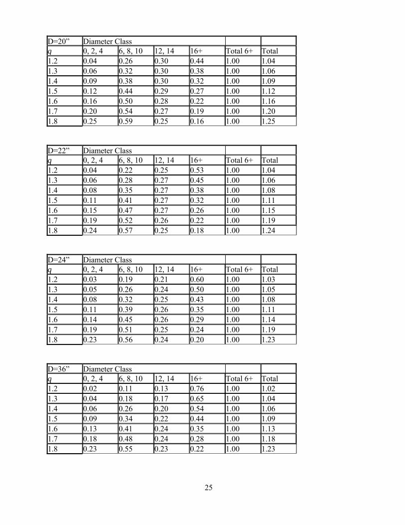
25

D=20” Diameter Class q 0, 2, 4 6, 8, 10 12, 14 16+ Total 6+ Total1.2 0.04 0.26 0.30 0.44 1.00 1.041.3 0.06 0.32 0.30 0.38 1.00 1.061.4 0.09 0.38 0.30 0.32 1.00 1.091.5 0.12 0.44 0.29 0.27 1.00 1.121.6 0.16 0.50 0.28 0.22 1.00 1.161.7 0.20 0.54 0.27 0.19 1.00 1.201.8 0.25 0.59 0.25 0.16 1.00 1.25 D=22” Diameter Class q 0, 2, 4 6, 8, 10 12, 14 16+ Total 6+ Total1.2 0.04 0.22 0.25 0.53 1.00 1.041.3 0.06 0.28 0.27 0.45 1.00 1.061.4 0.08 0.35 0.27 0.38 1.00 1.081.5 0.11 0.41 0.27 0.32 1.00 1.111.6 0.15 0.47 0.27 0.26 1.00 1.151.7 0.19 0.52 0.26 0.22 1.00 1.191.8 0.24 0.57 0.25 0.18 1.00 1.24 D=24” Diameter Class q 0, 2, 4 6, 8, 10 12, 14 16+ Total 6+ Total1.2 0.03 0.19 0.21 0.60 1.00 1.031.3 0.05 0.26 0.24 0.50 1.00 1.051.4 0.08 0.32 0.25 0.43 1.00 1.081.5 0.11 0.39 0.26 0.35 1.00 1.111.6 0.14 0.45 0.26 0.29 1.00 1.141.7 0.19 0.51 0.25 0.24 1.00 1.191.8 0.23 0.56 0.24 0.20 1.00 1.23 D=36” Diameter Class q 0, 2, 4 6, 8, 10 12, 14 16+ Total 6+ Total1.2 0.02 0.11 0.13 0.76 1.00 1.021.3 0.04 0.18 0.17 0.65 1.00 1.041.4 0.06 0.26 0.20 0.54 1.00 1.061.5 0.09 0.34 0.22 0.44 1.00 1.091.6 0.13 0.41 0.24 0.35 1.00 1.131.7 0.18 0.48 0.24 0.28 1.00 1.181.8 0.23 0.55 0.23 0.22 1.00 1.23

26

Uneven-aged Management in New England: Does It Make Economic Sense? Theodore E. Howard, Professor of Forestry Economics, Department of Natural Resources, University of New Hampshire, Durham, NH 03824, (603) 862-2700, tehoward@unh.edu Introduction Does uneven-aged management make economic sense in New England? This one-handed economist says, “Yes, but it is a matter of how much sense and how many cents.” The economics of forest management is complex and it is made even more so by intricacies of uneven-aged silviculture. Advances in modeling stand development and prescription responses ultimately led to practical management guides for practitioners. My goal is to remind us of economic principles that will help us evaluate alternatives whether from published guides or from the seats of our pants. Principles Economics, and especially forestry economics, is not about money. It is about how people make choices given limited resources. Survey research has shown that non-industrial private landowner objectives are rarely expressed in financial terms. Resource economists formally recognize that many values are not priced by the market and have developed methodologies to put un-priced values such as option, existence, and bequest values on an equal footing with money. In practical management situations, however, we generally rely on an implicit valuation of such things as biodiversity, wildlife habitat, and water quality. For example, given two management prescriptions, how much money will not be realized if additional timber is retained for snag tree recruitment? What is the opportunity cost of expanding the protection zone around vernal pools? Economics is all about money in the sense that financial analysis is important, even if it serves only to identify the opportunity costs associated with prescription alternatives. Further, while landowners may not have monetary objectives, they will certainly favor the most cost-effective means of achieving them. Ultimately, we cannot escape financial analysis and, therefore, it is important to remember some principles and practices. For now, we will assume that the biometricians and stand modelers have done their job informing us on matters of growth, yield, and stand development, as we peer into the monetary vernal pool to see what is hatching. The Analytic Framework of Forestry Economics Forests are natural and financial capital. In their role as natural capital, we are concerned with sustaining the stocks and flows of goods and services, outcomes and conditions. In their role as financial capital we struggle with how much capital to invest (the stocking question) and how long to invest that capital (cutting cycles and maximum diameter as a proxy for age). Stumpage and log markets are not perfectly competitive due to asymmetries in knowledge and the spatial distribution of forests and markets. Therefore, landowners may not be fully compensated for his or her forest management investments. Non-industrial landowners are generally price-takers, but may realize some price differentiation due to stumpage quality and bio-physical factors such as stocking and terrain. Regardless of the goals held by landowners, our use of financial analysis must recognize that economic efficiency is the means to those goals and not the goal itself. In the application of efficiency analysis, Net Present Value (NPV) is the best criterion for making financial decisions that require us to recognize the impact of time on valuation. A closely related criterion, Return on

27

Investment (ROI), works, too, because of its intuitive interpretation. ROI does requires a comparative benchmark discount rate (alternate rate of return) if it is to be used as a decision tool. Perhaps because of the relatively long time periods of investment that characterize forestry, one of the frequent errors made in financial analyses is the mixing of real and nominal prices and rates. Done correctly, prices, discount rates, and price change rates must be either all in nominal (with inflation included) or all in real (inflation excluded) terms. Mixing real and nominal values is a fatal error in financial analysis. In addition to the variability in biological measures and responses, uneven-aged ventures are subject to natural and financial risks. When is the next ice storm? What is going to happen to hemlock prices as the woolly adelgid migrates north? Risk and uncertainty in all of the biological, economic, and financial parameters of our decisions requires informed judgments. For analytical purposes, an appropriate method is calculating expected present net values based on assessments of likely future conditions. As an alternative, a risk premium can be incorporated into the discount rate. However, users of this method often over-adjust for risk. Factors influencing financial performance There are several key factors which influence the financial performance of any forestry investment, including the management of uneven-aged stands. Foremost among these factors is the biological growth rate. Slow growing stands rarely justify long-term investment and treatments that enhance growth are more likely to pay off. We also may expect that future stumpage prices will be higher than those of today. While price growth is not guaranteed, stumpage prices for the more valuable species and products have demonstrated modest real increases over long periods of time. In rough terms, one simply adds or subtracts the weighted average rate of price change to the ROI to account for future prices. Technically, one should multiply the constant price ROI by the rate of price change (RPC): (1 + ROI) * (1 + RPC) to obtain the actual ROI. However, the mathematical difference is small and there is enough uncertainty about future yields and prices to permit simple addition. Other speakers have noted the importance of the maintaining large poles and small sawlogs in uneven-aged treatments because these trees represent the biological future of the stand. These trees also contribute to financial performance due to movement in product class. Pulpwood size trees become small sawlogs and small sawlogs become large sawlogs and veneer allowing the landowner to realize higher prices per unit of volume. The discount rate used in the financial analysis is another major influence and they will vary with the circumstances of each landowner. The ROI of a management alternative will be compared to the hurdle rate appropriate for the landowner. Alternatives with returns greater than the hurdle rate are worth pursuing, however, the alternative with the highest ROI is not necessarily the most profitable. There are quirks in the mathematics that prevent such a universal declaration. Further, budget constraints may result in foregoing some worthwhile investments. Finally, the analytical results depend on forecasts of prices, response to treatment, product distribution, and other parameters. The further into the future such forecasts are made, the greater will be the uncertainty in the analysis.

28

Management Decisions The economic analytic framework is a decision support tool to help landowners and their advisors make management decisions about alternative uneven-aged prescriptions. Before any financial analysis is performed, landowners must formulate their goals and objectives. From those, we can derive our lists of desired species and product mix. We can also specify the target diameter distribution, stocking level, and maximum diameter. Finally, we can set our cutting cycle length, mindful of the need to balance frequency of income with growth in value and the opportunity to realize income from at-risk crop trees. Among the outcomes of the financial analysis will be guidance about which of the above goals and decisions are economically feasible. A Case Study in Mixed Hardwoods To illustrate the application of financial analysis, I have developed a case study using data from a mixed hardwood stand in southern New Hampshire. The stand is dominated by northern red oak, red and sugar maple, with minor amounts of hickory, ash, and beech. Hemlock and remnant emergent white pine provide the softwood component. For the purposes of this experiment, I assumed that the highest and best economic use of the land is forestry, as determined by economic geography or by legal conditions. Therefore, the decisions to be made are about alternative silvicultural prescriptions and not about alternative land uses. The per-acre stand characteristics are 120 square feet of basal area, 276 trees and 2,300 cubic feet, half of which is of sawlog quality. Diameters at breast height range from four to 26 inches. The initial value of the stand is $1,490 per acre. I assumed an annual growth rate of 3.8%, which is at the high end for New England. However, it is a lovely stand which would pay a lot of tuition bills. Approach Although this conference has not been very supportive of using q to determine preferred diameter distributions, I have done so to provide a systematic approach to the analysis. I varied the q-factor from 1.25 to 2.5 by increments of 0.25 and target basal areas (B*) of 120, 140, and 160 square feet per acre. Maximum diameter was set at 22 inches. Prices were assumed to be either constant throughout the analysis period or increased in real terms by two percent annually. Cutting cycle was set at ten years. Findings: timing is everything If the decision is to let a stand grow, then the target distribution is irrelevant. The initial stand will grow for the cycle and adjustments made to the stand at cycle-end will be such that harvest plus residual volumes and values will equal the projected volumes and values. If there is no expectation of higher or lower prices, ROI is influenced only by the biological growth rate, 3.82 percent in this case. If stumpage prices increase in real terms, one can simply add the rate of price change to the ROI. Technically, one should multiply the constant price ROI by the rate of price change (1+ROI) x (1+RPC) to obtain the dynamic price ROI. For example, if prices were expected to increase 2 percent annually, multiplication would yield 5.89 percent, a little more than simple addition (5.82 percent). As noted earlier, for practical purposes, given the uncertainty in prices, yields, and product mix, addition will provide a reasonable approximation.

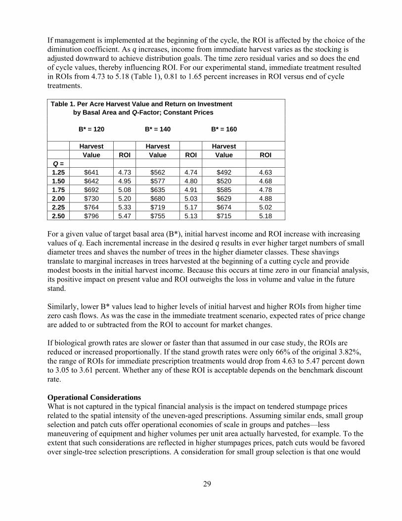
29

If management is implemented at the beginning of the cycle, the ROI is affected by the choice of the diminution coefficient. As q increases, income from immediate harvest varies as the stocking is adjusted downward to achieve distribution goals. The time zero residual varies and so does the end of cycle values, thereby influencing ROI. For our experimental stand, immediate treatment resulted in ROIs from 4.73 to 5.18 (Table 1), 0.81 to 1.65 percent increases in ROI versus end of cycle treatments. Table 1. Per Acre Harvest Value and Return on Investment by Basal Area and Q-Factor; Constant Prices B* = 120 B* = 140 B* = 160

Harvest Harvest Harvest

Value ROI Value ROI Value ROI Q = 1.25 $641 4.73 $562 4.74 $492 4.63 1.50 $642 4.95 $577 4.80 $520 4.68 1.75 $692 5.08 $635 4.91 $585 4.78 2.00 $730 5.20 $680 5.03 $629 4.88 2.25 $764 5.33 $719 5.17 $674 5.02 2.50 $796 5.47 $755 5.13 $715 5.18

For a given value of target basal area (B*), initial harvest income and ROI increase with increasing values of q. Each incremental increase in the desired q results in ever higher target numbers of small diameter trees and shaves the number of trees in the higher diameter classes. These shavings translate to marginal increases in trees harvested at the beginning of a cutting cycle and provide modest boosts in the initial harvest income. Because this occurs at time zero in our financial analysis, its positive impact on present value and ROI outweighs the loss in volume and value in the future stand. Similarly, lower B* values lead to higher levels of initial harvest and higher ROIs from higher time zero cash flows. As was the case in the immediate treatment scenario, expected rates of price change are added to or subtracted from the ROI to account for market changes. If biological growth rates are slower or faster than that assumed in our case study, the ROIs are reduced or increased proportionally. If the stand growth rates were only 66% of the original 3.82%, the range of ROIs for immediate prescription treatments would drop from 4.63 to 5.47 percent down to 3.05 to 3.61 percent. Whether any of these ROI is acceptable depends on the benchmark discount rate. Operational Considerations What is not captured in the typical financial analysis is the impact on tendered stumpage prices related to the spatial intensity of the uneven-aged prescriptions. Assuming similar ends, small group selection and patch cuts offer operational economies of scale in groups and patches—less maneuvering of equipment and higher volumes per unit area actually harvested, for example. To the extent that such considerations are reflected in higher stumpages prices, patch cuts would be favored over single-tree selection prescriptions. A consideration for small group selection is that one would

30

also expect lower levels of damage to the residual stand which translates to higher quality trees for the next cutting cycle. Key Points Uneven-aged management of New England forests does make economic sense, particularly when economics is seen as making choices. Financial analysis can guide us in making economically efficient choices and in bounding opportunity costs of alternatives. Returns on investment depend on the biological growth rates of forests, the timing of harvests, forecasts of prices and yields and operational details. If this one-handed economist could find another hand, I would applaud your efforts to practice better uneven-aged silviculture.

31

Uneven-aged Management of Northern Hardwoods William B. Leak, Northern Research Station, 271 Mast Road, Durham, NH 03824, bleak@fs.fed.us The northern hardwood type includes American beech, yellow birch, sugar maple, and associated species such as red maple, paper birch, white ash, and minor amounts of softwoods such as hemlock. Uneven-aged management in northern hardwoods includes both individual-tree selection and group/patch selection. I'll discuss both. These two systems provide for a fairly light touch on the landscape, and therefore are useful on small private ownerships and sensitive areas where heavier harvesting systems would be intrusive. However, other systems such as clearcutting and shelterwoods—especially delayed shelterwoods—also are optimal under the right circumstances. Individual Tree Selection Individual-tree selection is the removal of single trees, including trees throughout the range in diameter classes when commercially feasible. In northern hardwoods, a residual stand of perhaps 60 to 80 square feet basal area per acre is reasonable. The residual stand should contain a component of poletimber and sawtimber that will provide for another commercial cut in 15 to 20 years. The system provides for repeated timber yields from a single stand. Fifty years of experience from the Bartlett Experimental Forest shows that stand quality steadily increases, even from a stand such as this that was heavily infected by the beech-bark disease in the 40's and 50's (Leak and Sendak 2002):

Tree Grade 1952 1976 2000 (percent of sawtimber volume)

1&2 29 42 45 3 50 31 40 5 14 26 11 Cull 7 1 3

The optimum stocking and structure of the residual stand has been the subject of much debate over the years. The concept of q—the constant ratio (making it J-shaped) between numbers of trees in successively smaller DBH classes has been described earlier in this proceedings. An example of the relationship between q and the basal area in poles and sawtimber is outlined below:

Size Class Q=1.7 Q=1.3 (basal area per acre) Poletimber 38 21 Sawtimber 32 49 Total 70 70

One theory says that q-objectives for the residual stand should be low, therefore providing high levels of sawtimber and, presumably, high levels of sawtimber growth. A complementary theory says that the residual stand should closely resemble the ideal q -type or J-shaped form. Let's examine these: A comprehensive growth study on the Bartlett Experimental Forest showed that some of the best sawtimber growth over a 10-year period following treatment was produced by residual stands with

32

60 to 80 square feet residual basal area with only about 25 to 35 square feet sawtimber—equivalent to a q of about 1.7 (Leak 2003b). This was a stand of only moderate quality—primarily beech, red maple, and birches—growing on a mediocre site. These sites apparently will not support high basal areas of sawtimber or large trees; there are sites that will support larger, higher basal areas of sawtimber. Our conclusion has been that the appropriate basal areas of poletimber and sawtimber depend on and vary with site and tree vigor/quality:

Stand BA Sawlog BA Sawlog BA Growth

(basal area in square feet per acre) 40 18 .43 60 27 .76 36 .76 80 24 .64 32 .49 45 .37 100 60 .60

As indicated in the table above, one treatment with 100 square feet residual and 60 square feet sawtimber also produced relatively high sawtimber growth. However, this treatment would allow for a very light cut, and the ingrowth (recruitment) of trees into the sawtimber size classes was low. Another interesting facet was that stands cut to a very non-J-shaped distribution rebounded to an essentially J-shape over the next 25 years due to rapid regeneration and ingrowth (Leak and Gove 2006). Similar findings have come from computer simulation studies and longterm monitoring of diameter-limit cuts (Leak 1996 and 2002). In addition, there are non-J-shaped forms (slightly S-shaped for example) that might be more productive than the J-shape. Another notion on diameter distributions: decades ago, Adrian Gilbert (silviculturist/economist) told me that a stand's diameter distribution should be regarded as a result of the marking practices used instead of an objective. In other words, if you (1) regenerate the stand properly, (2) maintain moderate stand density so that the poletimber develops rapidly, and (3) retain sufficient quality sawtimber for rapid growth and a future harvest in 15 to 20 years, then a sustainable diameter distribution will develop that is in sync with the marking practices, site, stand composition, etc. It might be J-shaped, sigmoid or a combination of the two. The bottom-line for individual-tree selection seems to be: mark the stand well, leaving 60 to 80 square feet of basal area in trees with good potential, with as little as 25 to 35 square feet in sawtimber—more if the quality is good. Lower stocking is advisable for longer intervals between harvests (Nyland 1998). Don't worry too much about the J-shape. In addition, make sure that the regeneration is in the species you want since individual-tree selection (or any partial cut) will produce mostly tolerant species—sometimes mostly beech and hemlock as indicated from longterm records on sapling understories on the Bartlett Experimental Forest: Method Beech Yellow birch Sugar maple Red maple Hemlock (percent of sapling numbers) Diameter Limit 33 - 6 - 61 Individual Tree Selection 56 2 5 2 35

33

Group/Patch Selection To still practice uneven-aged management on sites that have more tolerant species than desired, we urge the use of group/patch selection using openings of around 1/4 to 1/2-acre or even several acres on large industrial ownerships. They are located in areas where there are groups of mature/defective stems, especially with undesirable understories. The system is managed by area control, e.g. for a 100-year rotation and an entry every 20 years, no more than 20% of the stand would be harvested in patches. Marking could occur between the patches, or not, depending upon the desire to produce more timber versus leaving more area undisturbed to accumulate coarse woody debris. One example of the regeneration produced (at 47 years) on a series of patches cut in 1954 on a mediocre beech-red maple site on the Bartlett Experimental Forest is shown below (Leak 2003a). The understory of this stand was almost pure beech, and the once-abundant pin cherry had mostly died: Size Class Beech Yellow birch Sugar maple Red maple Paper birch White ash Red spruce Hemlock (percent of basal area) 5-inch + 26 17 3 15 34 2 2 1 8-inch + 9 19 3 27 39 3 - - Typically, a patch in northern hardwoods is like a small clearcut that removes most of the understory through logging disturbance. However, the system also can be used to release desirable understories through removal of the overstory; this approach probably is more accurately termed a group rather than a patch. Another interesting sidelight on the use of group/patches or even larger clearcuts is that the understory, after about 30 to 40 years, tends to have richer species than in areas outside the opening (Leak 2005); this could be due to the higher foliar nutrient contents of the early successional species that regenerate in openings—pin cherry, aspen, etc.: Stand Beech Sugar maple Red maple White ash other (understory stems per acre 2 to 4 feet tall) Uncut 1082 58 29 - - Patches 900 2004 58 29 29 Literature Cited Leak, W.B. 1996. Longterm structural change in uneven-aged northern hardwoods. For. Sci. 42:160-165. Leak, W.B. 2002. Origin of sigmoid diameter distributions. YSDA Forest Service Res. Paper NE-718, 10 p. Leak, W.B. 2003a. Regeneration of patch harvests in even-aged northern hardwoods in New England. North. J. App. For. 20(4):188-189. Leak, W.B. 2003b. Best density and structure for uneven-aged northern hardwood management in New England. North. J. Appl. For. 20(1):43-44 Leak, W.B. 2005. Effects of small patch cutting on sugar maple regeneration in New Hampshire northern hardwoods. North. J. Appl. For. 22(1):68-70. .Leak, W.B. and P.E. Sendak. 2002. Changes in species, grade, and structure over 48 years in a managed New England northern hardwood stand. North. Jour. Appl. For. 19(1):25-27. Leak, W.B. and J.H. Gove. 2006. Growth of northern hardwoods – a 25-year update. (in review). Nyland, R.D. 1998. Selection system in northern hardwoods. J. For. 96:18-21.

34

Uneven-Aged Silviculture Research on the Penobscot Experimental Forest Laura S. Kenefic and John C. Brissette, USDA Forest Service, Northern Research Station, Bradley, ME and Durham, NH Introduction The Penobscot Experimental Forest (PEF) in central Maine is the site of a long-term study of uneven-aged silviculture initiated in the early 1950s. The selection system has been applied on different cutting cycles in replicated stands averaging 20 acres in size for over 50 years. Remeasurements have been made on permanent plots with individually numbered trees before and after every harvest, and at 5-year intervals between harvests. The PEF thus provides a rare long-term perspective on the dynamics of managed uneven-aged stands (Kenefic et al. in press). The PEF is located in the Acadian Forest, a transition between the eastern broadleaf and boreal forests. The study stands are dominated by shade-tolerant northern conifer species such as balsam fir, spruce species, and eastern hemlock, in mixture with northern white-cedar, eastern white pine and hardwoods such as maple, birch, and aspen. These complex stands, which are characterized by small-scale natural disturbances, appear to be well-suited to the application of the selection system. Methodology Selection cutting has been applied on 5-, 10-, and 20-year cutting cycles with a residual structural goal defined using the BDq method. This means that there is a target residual basal area (B, or BA), maximum diameter (D) and q-factor (q). The q-factor is a mathematical method of defining the target number of trees in each diameter class. It results in a reverse-J diameter distribution, i.e. decreasing number of trees per acre over increasing diameter. Treatments on the PEF began as single-tree selection, but changed to a combination of single-tree and small group (2 to 3 tree) removals approximately 30 years into the study. Target residual BA (trees ≥0.5 inches DBH) ranges from 80 ft2/ac in the 20-year cutting cycle to 115 ft2/ac in the 5-year cutting cycle, and maximum diameter ranges from 16 to 19 inches DBH (Sendak et al. 2003). Prior to each treatment the stand is inventoried to determine the number of trees in each diameter class, and the amount of basal area available for harvest. Marking guidelines are used to prioritize removals, which are distributed across diameter classes that have excesses relative to the structural goals. Stems < 50% merchantable by volume are the first to be cut, followed by trees expected to die before the next entry, undesirable species, and trees beyond financial maturity (maximum diameter). We also endeavor to release crop trees on three sides and create or enlarge regeneration openings. Species composition goals also guide removals. Our targets are 35 to 55% of BA in spruce species, 15 to 25% each in balsam fir and eastern hemlock, and 5 to 10% each in pine, paper birch, cedar, and other. Findings Though the diameter distributions are somewhat unbalanced, with poletimber deficits and sawtimber surpluses, tree size diversity is great. There are some questions about the ecological basis for the mathematical structure, and the goal is currently being revised to reflect species-specific growth rates and mortalities. The relationships between tree age and size are generally weak, particularly for red spruce (Seymour and Kenefic 1998). This is not uncommon in shade-tolerant species, which can grow for extended periods of time beneath the overstory. Though trees of shade-tolerant species generally respond well to release at advanced ages, we still need to grow enough new trees at a fast

35

enough rate to sustain a managed stand. Though regeneration is prolific (Brissette 1996), ingrowth into the sapling classes is slow (Kenefic and Brissette 2005). Efforts to release understory trees are important, particularly for spruce, which is outcompeted in the understories of these stands by hemlock at the lowest light levels and fir at moderate to high light levels (Moores et al. 2004, in preparation). Comparison of the selection stands to variants of diameter-limit cutting on the PEF support the conclusion that all partial cuts are not the same. Repeated fixed diameter-limit cutting resulted in less sawtimber growth and volume, less regeneration, less residual value and more cull than selection cutting (Kenefic et al. 2005, Kenefic and Nyland 2005). A compromise treatment, using flexible diameter thresholds, shows some promise (Kenefic et al. 2004, 2005), though current structures suggest that similarities between this system and selection may be due to an abundance of small trees which are soon to be cut as they pass the threshold for removal. Highlights Selection cutting maintains diversity of tree ages, sizes, and species. The PEF experiment suggests that a combination of single-tree and small group removals is effective in northern conifers, likely due to the need for some larger openings to release established, suppressed regeneration. The PEF experiment suggests that there are benefits to considering component species individually, due to differential growth rates and longevities (Kenefic et al. in preparation). The bottom line is that though the structures are somewhat unbalanced, the stands are healthy, diverse, well-stocked and well regenerated (Figure 1). Treatments that remove low vigor, poor quality trees and undesirable species across all size classes, maintain a diversity of tree sizes and ages, and create openings to establish and release regeneration are likely to be successful in northern conifer stands. This is a brief overview of the PEF selection cutting experiment. Additional information can be found in the cited literature, and will be presented in upcoming journal papers by Kenefic and others. Literature Cited Brissette, J.C. 1996. Effects of intensity and frequency of harvesting on abundance, stocking and composition of natural regeneration in the Acadian Forest of eastern North America. Silva Fennica 30(2-3):301-314. Kenefic, L.S., J.C. Brissette, and P.E. Sendak. 2004. The effects of alternative diameter-limit cutting treatments: Some results from a long-term northern conifer experiment. In: Proceedings of the 84th Annual Winter Meeting of the New England Society of American Foresters. Gen Tech. Rept. NE-314. Newtown Square, PA: U.S. Department of Agriculture, Forest Service, Northeastern Research Station: 22-24. Kenefic, L.S. and Brissette, J.C. 2005. Sapling recruitment and growth dynamics in uneven-aged northern conifer stands: A 20-year study. In: Kenefic, L.S. and Twery, M.J. (eds). Changing Forests – Challenging Times. Proceedings of the 85th Winter Meeting of the New England Society of American Foresters. Gen Tech. Rept. NE-325. Newtown Square, PA: U.S. Department of Agriculture, Forest Service, Northeastern Research Station: 55. Kenefic, L.S. and R.D. Nyland. 2005. Diameter-limit cutting and silviculture in northeastern forests: a primer for landowners, practitioners, and policy makers. NA-TP-02-05. Newtown Square, PA: U.S. Department of Agriculture, Forest Service, Northeastern Area. 18 p. Kenefic, L.S., J.C. Brissette, and P.E. Sendak. 2005. Long-term study of northern conifers provides new perspectives on partial cutting alternatives. In: Proceedings of the Fifth North American Forest Ecology Workshop. 12-16 June 2005. Gatineau, Quebec:126.

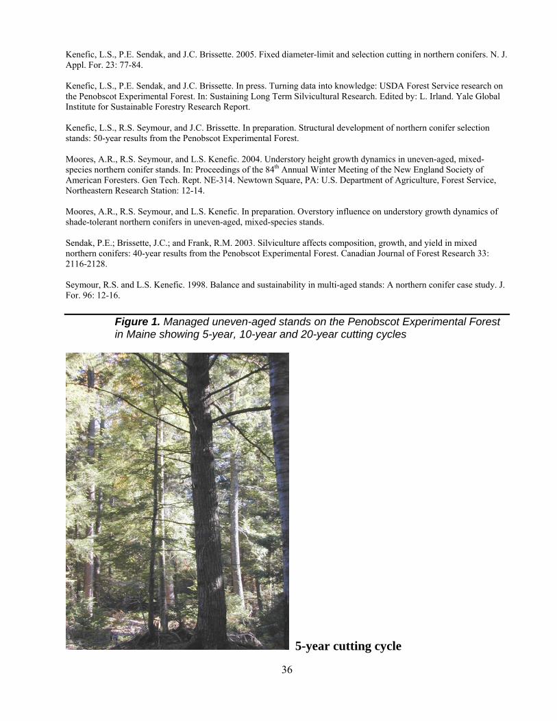
36

Kenefic, L.S., P.E. Sendak, and J.C. Brissette. 2005. Fixed diameter-limit and selection cutting in northern conifers. N. J. Appl. For. 23: 77-84. Kenefic, L.S., P.E. Sendak, and J.C. Brissette. In press. Turning data into knowledge: USDA Forest Service research on the Penobscot Experimental Forest. In: Sustaining Long Term Silvicultural Research. Edited by: L. Irland. Yale Global Institute for Sustainable Forestry Research Report. Kenefic, L.S., R.S. Seymour, and J.C. Brissette. In preparation. Structural development of northern conifer selection stands: 50-year results from the Penobscot Experimental Forest. Moores, A.R., R.S. Seymour, and L.S. Kenefic. 2004. Understory height growth dynamics in uneven-aged, mixed-species northern conifer stands. In: Proceedings of the 84th Annual Winter Meeting of the New England Society of American Foresters. Gen Tech. Rept. NE-314. Newtown Square, PA: U.S. Department of Agriculture, Forest Service, Northeastern Research Station: 12-14. Moores, A.R., R.S. Seymour, and L.S. Kenefic. In preparation. Overstory influence on understory growth dynamics of shade-tolerant northern conifers in uneven-aged, mixed-species stands. Sendak, P.E.; Brissette, J.C.; and Frank, R.M. 2003. Silviculture affects composition, growth, and yield in mixed northern conifers: 40-year results from the Penobscot Experimental Forest. Canadian Journal of Forest Research 33: 2116-2128. Seymour, R.S. and L.S. Kenefic. 1998. Balance and sustainability in multi-aged stands: A northern conifer case study. J. For. 96: 12-16.

Figure 1. Managed uneven-aged stands on the Penobscot Experimental Forest in Maine showing 5-year, 10-year and 20-year cutting cycles

5-year cutting cycle

37

10-year cutting cycle

20-year cutting cycle

38

Uneven-aged Management for Oak and Pine Forest Types in Southern New England

Matthew J. Kelty, Department of Environmental Conservation, University of Massachusetts, Amherst MA 01003 Background Most of the papers in this conference have described uneven-aged management methods as applied to northern hardwoods and spruce-fir-hemlock stands. This paper differs in that it focuses on stands in which red oak and white pine are the key species of interest for timber and/or wildlife management. These stands are mainly found in the transition hardwood-white pine-hemlock forest type (Westveld 1956), and are located in more southerly areas of New England or at lower elevations. Most of the ideas presented in this paper about selection methods in oak-pine stands have been described in more detail in Kelty et al. 2003. Uneven-aged management is most straightforward when applied to forest types in which the desired species are shade-tolerant and are readily established as advance regeneration. Sugar maple and red spruce are good examples of such species. Even then, selection methods are not necessarily simple because of issues such as animal damage to regeneration, interfering understory plants, and logging damage during the selection harvests. The situation with white pine and red oak is even more complicated because these species are low in shade-tolerance and regenerate only periodically when mast seed years occur. The seedlings have slow initial height growth, but after reaching 3 to 6 feet in height, they grow very rapidly in full sunlight—matching the growth rates of pioneer species. In many stands, a stratified structure develops, with pine, oak, black cherry, and white ash forming an upper canopy above more shade-tolerant species such as red maple and black birch (Kelty 1986, Stephens and Ward 1992). The shelterwood method appears to be the most logical to recreate the composition and structure of the mature oak- and pine-dominated stands, and it has been used successfully throughout the region (Hannah 1988, Seymour 1995). The shelterwood overstory moderates moisture and temperature conditions for establishment and early growth; then when the regeneration is capable of rapid growth, the overstory removal provides full sun. However, many landowners seek alternative methods, even if these methods are not necessarily tied closely to the ecological characteristics of the species. Many private woodlot owners live on or near their land and are primarily interested in conservation, rural landscape beauty, and recreation goals (Rickenbach et al. 1998). They want to minimize the amount of disturbance associated with harvests, so the use of even-aged methods, especially with two or more cuts in shelterwoods, are often not acceptable. Various kinds of selection cutting or diameter-limit cutting (including high-grading) are used because all of these harvests remove fairly high-value trees with relatively low disturbance. Most private landowners can't distinguish among these partial cuts, but there are many foresters who are interested in assuring that selection is used instead of high-grading. In addition to the interests of family forest owners, managers of some public watershed forests have defined uneven-aged stands as the desired future goal for their lands, to minimize the area disturbed at any one location and to vary the height structure of the stands to reduce the risk of widespread blowdown—all to protect water quality (Barten et al. 1998). Thus, there is considerable interest in applying the selection system to stands in the transition hardwood-white pine-hemlock type. Often this consists of the first step in the conversion of even-aged stands to uneven-aged structure, because most stands are relatively even-aged, having become established after heavy cutting or hurricane damage.

39

Objectives The objectives of this paper are to review the research on two main silvicultural problems that arise when planning for the use of the selection method: 1) Establishing regeneration in some portions of the stand, and 2) Regulating the overall level of cutting within the stand. The main questions are: 1) What size of canopy openings should be made and what range of tree sizes should be cut within

the openings to obtain regeneration of the desired species? 2) How should the overall level of cutting be controlled within the stand: by the use of target

diameter distributions (such as BDq concepts), by establishing a certain portion of the stand area to be harvested in each cutting cycle, or by some combination of the two?

Few silvicultural studies in the transition hardwoods forest type have included selection methods. However, detailed studies of some of these questions have been carried out in northern hardwood forests in northern New England, and in central Appalachian hardwoods to the south, primarily on experimental forests of the USDA Forest Service. General results from these studies in adjacent regions can be applied to southern New England forests with care taken to account for differences in species composition among the regions. Size of canopy openings Because shading of canopy openings by adjacent mature trees is a major factor that affects regeneration, one important consideration of harvest gap size is the distance that the edge effect extends into the gap (Bradshaw 1992). For this reason, the diameter of a harvest gap is often expressed in terms of the height of surrounding trees. The following relation of gap diameter to area is useful for reference, assuming a tree height of 80 feet and circular openings:

1 tree height = 0.1 acre 2 tree heights = 0.5 acre 3 tree heights = 1.0 acre

The traditional silvicultural terms that relate to opening size in selection harvests are very simple: 'single-tree selection' is used for a gap size of one tree crown in diameter (about one-half tree height or less, or about 0.03 ac), and 'group selection' is used for any gap size larger than that. A number of studies have directly examined the effect of opening size on species composition and growth of regeneration. The largest of these was conducted on five USDA Forest Service experimental forests in the central hardwood type, in West Virginia, southern Ohio, Kentucky, and southern Illinois (Dale et al. 1995). Although the species composition of these forests differs considerably from that of New England stands, the principles of the effects of opening size on groups of species categorized by shade-tolerance are applicable. Sizes of openings ranged from 0.04 to 1.6 acres, and all trees in the openings were cut to a minimum DBH of 3 to 5 inches, with smaller vegetation either cut or treated with herbicide. Regeneration was assessed 30 years later on sample plots located at varying distances from the edge to the center of the opening. Results showed that the greatest shift in species composition occurred between opening sizes of 0.1 acre and 0.3 acre. Shade-tolerant species dominated the plots close to the edge (less that 20 feet), and this edge effect accounted for nearly the entire area of openings up to 0.1 acre. Plots in the center of 0.3-acre openings developed equal stem densities of intolerant and tolerant species. In larger openings, edge plots were still dominated by tolerant species, and the ratio of intolerant to mid-tolerant to tolerant

40

species remained constant across plots at varying distances farther into the center. However, height and diameter growth of trees (particularly of less tolerant species) in the centers did continue to increase with increasing opening size to the largest in the study. Thus, the young stands were developing stratified canopy structure at age 30 in the more open parts of the harvest gaps. The effects of opening size on regeneration composition in northern hardwoods were summarized by Lamson and Leak (2000). The trends matched the results described above, with openings less than 0.1 acre being dominated by tolerant species (sugar maple and beech), those from 0.2 to 0.5 acre having 25% of total stem density comprised of yellow birch, paper birch, and white ash, and those from 0.7 to 1.0 acre with 40 to 50% of the less tolerant species. Choice of trees to be cut within canopy openings Any size of harvest opening can be made by cutting only the overstory trees, or by cutting both overstory and lower canopy trees. This distinction is included in silvicultural terminology by adding a third selection method to the two already mentioned. Thus, the three terms are: single-tree selection, group selection, and patch selection (Leak and Filip 1975). In single-tree and group selection, only overstory trees are cut, with the choice between the two depending on whether mature trees tend to occur singly or in groups. It is understood in the general concept of these methods that smaller trees are cut throughout the stand to release young desirable trees from competition, but the smaller trees to be cut are not necessarily within the openings made by the harvest of mature trees (and often in practice, no small trees are cut at all). Patch selection differs in that it adapts the patch clearcutting method to the uneven-aged system. The range of sizes for patch cuts can be the same as the range for group cuts, but the key differences are that patch size is predetermined rather than depending on the size of groups of mature trees, and that all trees down to a small diameter (usually 1 or 2 inch DBH) are cut within the opening. There seems to be some confusion in putting the results of research on opening size into management practice. In the studies described above, all trees down to 1 inch were removed, so they represented patch selection cuts. But often in practice, large selection cuts are made to establish regeneration of less tolerant species but without cutting midstory and understory trees in the harvest areas. A demonstration study was established in Massachusetts in 1988 to examine the importance of removing smaller trees on establishment and growth of regeneration (Kelty et al. 2003). The study compared regeneration in selection cuts and shelterwood cuts in a mature stand comprised mainly of red oak, white pine, red maple, black birch, and mountain-laurel. The shelterwood cutting reduced the overstory to a basal area of 60 ft2/ac, and the selection cuts were circular gaps of 0.3 acre in size. The understory (all trees and shrubs less than 6 inch DBH) was cut in half the plots and retained in the other half in each cutting type. Ten years after cutting, species composition of regeneration was similar in all plots; red oak and red maple were the most abundant in all. White oak, black birch, white pine, and chestnut were present at lower densities. The greatest stem density of all species combined was found in the shelterwood plots in which the understory had been removed. Selection cuts had lower total seedling densities with a lower proportion of oak, regardless of understory treatment. However, considering only regeneration greater than 5 feet in height, the patch cuts had greater seedling densities of oak and of all species combined, compared to shelterwood plots. The greatest density of tall oak regeneration was in the selection cuts with the understory removed (that is, the patch cuts). These results confirm those of the more extensive studies described above, which have shown that 0.3-acre patches are large enough to allow species of low and intermediate shade-

41

tolerance to become established. They also indicate the importance of removing small trees and shrubs for obtaining high seedling densities that can develop rapidly in height. Control of cutting at the stand level Uneven-aged stands can be managed, at least conceptually, like a sustained-yield forest on a small scale; these are referred to as balanced uneven-aged stands. The simplest method at the forest level is to use area control to develop a balanced forest—that is, to create equal areas of stands of each age class. However, when the harvest of mature trees is restricted to single trees or small groups or patches, it is impractical to measure and keep track of the area harvested. Therefore, the use of target diameter distributions as a form of volume control of cutting has been favored. These methods have been described in detail in earlier papers in this conference. One of the problems with the use of diameter distributions has been the lack of a method to choose the appropriate target distribution. No matter how the target diameter distribution is chosen, the problem of the time involved with the detailed inventory and marking guides still exists. Methods have been developed to convert marking guides from 2-inch diameter classes into three to five broad diameter classes to use as a marking guide (Leak and Gottsacker 1985, Nyland 2002). Even with this simplification, the method becomes difficult when using group or patch selection—it is necessary to combine diameter-class marking guides with a tally of the area in groups. Experience has shown that this combined method becomes difficult with groups or patches larger than 0.1 acre (Leak and Gottsacker 1985). Because the cutting level in the patches is clearly heavier than indicated by the marking guide, the rest of the stand would have to be have to be cut more lightly than the guide in order for the stand to meet the target distribution overall; thus, no part of the stand would be cut to the target diameter distribution. With large patches of the size needed for regeneration of less tolerant species, it may be more logical to return to the original concept of relying entirely on area control (Leak 1999). For a given stand area, cutting cycle, rotation age, and average patch area, it is possible to calculate the number of patches to be cut and to use patch diameter to lay out the cutting areas. The stand area between the patches can be thinned during the same stand entry. Since this non-patch part of the stand is not being regenerated during this entry, even-aged thinning or improvement cutting methods are appropriate. Conclusion This review of patch cutting studies in the Northeast leads to the following suggestions for applying selection methods to transition hardwoods in order to favor oaks and white pine. 1) Canopy openings should be 0.3 acre or larger if the goal is to promote regeneration of intolerant

and mid-tolerant species in addition to shade-tolerant species. 2) These openings should be made as patch cuts rather than group cuts. The important aspect is that

all or most of the competing midstory and understory trees should be cut within the openings, while any desired advance regeneration present in the openings is retained. The objective of releasing established advance regeneration can often be an important factor in choosing the placement of the patch cuts.

3) Diameter-distribution guides have not proven very useful for determining selection cutting levels when using large patch cuts. Controlling the cut by allocating the proportion of stand area to be in patches is more straightforward and more likely to create the desired stand structure. Thinning between the patches can be carried out, but it is not a necessary part of the method.

42

4) With large patches, it may be desirable to leave one or more overstory reserve trees within the patch for habitat, aesthetics, or seed production, and thus treat each patch as a small-scale shelterwood or clearcut-with-reserves.

References Barten, P.K., T. Kyker-Snowman, P.J. Lyons, T. Mahlstedt, R. O'Connor, and B.A. Spencer. 1998. Managing a watershed protection forest. J. For. 96(8):10-15. Bradshaw, F.J. 1992. Quantifying edge effect and patch size for multiple-use silviculture--a discussion paper. For. Ecol. Manage. 48:249-264. Dale, M.E., H.C. Smith, and J.N. Pearcy. 1995. Size of clearcut opening affects species composition, growth rate, and stand characteristics. USDA For. Serv. Res. Pap. NE-698. 21 p. Hannah, P.R. 1988. The shelterwood method in northeastern forest types: A literature review. North. J. Appl. For. 5:70-77. Kelty, M.J. 1986. Development patterns in two hemlock-hardwood stands in southern New England. Can. J. For. Res. 16:885-891. Lamson, N.I. and W.B. Leak. 2000. Guidelines for applying group selection harvesting. USDA For. Serv. Northeastern Area State Priv. For. Publ. No. NA-TP-02-00. 8 p. Leak, W.B. 1999. Species composition and structure of a northern hardwood stand after 61 years of group/patch selection. North. J. Appl. For. 16:151-153. Leak, W.B., and S.M. Filip. 1975. Uneven-aged management of northern hardwoods in New England. USDA For. Serv. Res. Pap. NE-332. 15 p. Leak, W.B., and J.H. Gottsacker. 1985. New approaches to uneven-age management in New England. North. J. Appl. For. 2:28-31. Nyland, R.D. 2002. Silviculture: concepts and applications. McGraw-Hill, New York. 633 p. Rickenbach, M.G., D.B. Kittredge, D. Dennis, and T. Stevens. 1998. Ecosystem management: capturing the concept for woodland owners. J. For. 96(4):18-24. Seymour, R.S. 1995. The northeastern region. P. 31-79 in Regional silviculture of the United States, (3rd ed.), J.W. Barrett (ed.). Wiley, New York. Westveld, M. 1956. Natural forest vegetation zones of New England. J. For. 54:332-338.

43

Selection System Silviculture Experiments at the Caroline A. Fox Research Forest Kenneth Desmarais, Administrator – Forest Management, N.H. Division of Forests and Lands, kdesmarais@dred.state.nh.us Abstract – Selection silviculture is a topic that many foresters talk about but probably few truly practice. There has been little research on selection silviculture practices in the oak-pine forest type. Consequently, the Fox Research Forest staff decided to conduct several practices and monitor their performance with fixed area permanent plots to evaluate and gain practical experience with the practices. Introduction Many foresters talk about selection silviculture in New England but our experience suggests that few foresters truly practice it. Many practices may be truly classified as “free thinnings1” because after several of these cuttings foresters commonly look for ways to regenerate the stand. This indicates that the foresters were practicing some unregulated form of even-aged management because regeneration was not a priority until the stand neared maturity. Rarely do local foresters discuss stand structure whether intending toward a q or any other diameter or age class distribution or acres (or percent) of regeneration as in “group selection” cutting. Since the Caroline A. Fox Research and Demonstration Forest is the State of New Hampshire’s chief location for experimentation and education, it was decided that several selection system cuttings as well as other partial cutting applications be demonstrated and monitored for long term performance. Eight different treatments were established in the oak-pine forests of the tract and are being monitored with fixed area permanent plots. The methods are only briefly described below since other papers in these proceedings provide more details to the methods in general.

Methods Used

Stand 12A – Single tree selection (high density) was prescribed for this stand. The residual density is high (basal area= 130 ft²/ac) in anticipation of regenerating tolerant species, especially softwoods such as hemlock, red spruce and white pine. These species are consistent with site capabilities. The maximum DBH to grow is 20 inches and the desired q is 1.3 in order to maintain a stand high in sawtimber. The graph showing the pre-cut stocking versus the stocking goal reveals that the large sawtimber was much too numerous and the smaller size classes were much too few.

1 Smith, David M. 1962 The practice of silviculture. Wiley & Sons.

Fox Forest Stand 4-12

0

10

20

30

40

50

60

70

20 18 16 14 12 10 8 6

dbh

tree

s p

er a

cre

q = 1.3

presentstructure

44

Stand 31 – Single tree selection (low density) was conducted in this stand. The silvicultural goals are to develop and maintain a stable stand structure and to promote species with a wide range of shade tolerance including a greater percentage of white pine and red oak. The residual basal area goal is 80 ft² /ac. The maximum stem size is 20 inches DBH and the q structure is 1.3 to maintain a high stocking of sawtimber. Stand 32 – This stand is being managed as two different stands. Stand 32A is managed by aesthetic high-grading. Markers were instructed to reduce the basal area to 80 ft²/ac by removing the best quality stems. The stem quality of the residual stand will be tracked over time to study whether high-grading lowers the overall stem quality over time. The residual stocking is high enough to leave a well-stocked stand, which lay observers seem to rely most upon to evaluate “good forestry.” This demonstration is expected to yield interesting results. Stand 32B demonstrates group selection cutting. Group sizes are approximately ¼ to ½ acre. Groups focus on removing high-risk areas, over-mature timber and low-quality timber. Crop tree release was used to re-allocate resources to fewer but better quality trees and wildlife trees between group clearings. Crop tree spacing is 20 feet for softwoods and 30 feet for hardwoods. Stand 35 – Narrow strip cuttings are prescribed for this stand. The strips are expected to provide space for regeneration. These strips will be narrower than traditional strip cuts to provide an environment similar to shelterwood cutting. Strip widths will be 33 feet wide (1/2 chain) and will run in an east-west direction to provide part of the strip with direct sunlight and part with light shade. Stand 36 – Modified diameter limit cutting took place in this stand. All softwood trees greater than 15 inches DBH and all hardwood trees greater than 17 inches DBH were harvested. In order to attempt to improve the stand all unacceptable growing stock trees2 greater than 10 inches were harvested. Stand 37 – Multi-cohort management was prescribed for this stand. Multi-cohort management endeavors to manage the forest in distinct layers or strata. Each stratum toward the forest floor increases in the number of trees carried. The cohorts are established from cutting events of such intensity that regeneration is established and its development is permitted. Six cutting cycles are intended for this stand in a normal 120 year rotation. Forty year regeneration cycles establish three age classes or cohorts; age 0 – 40, 40 – 80 and 80 – 120 years. This stand presently contains a gap in age structure and consequently the management is adapted to facilitate a smooth transition. The relative density of growing space will be shared equally between

2 Unacceptable growing stock refers to all trees which do not or are not capable of someday containing sawtimber.

Fox Stand 31

0

10

20

30

40

50

60

20 18 16 14 12 10 8 6

dbh

tre

es

pe

r ac

re

goal

presentstructure

45

two cohorts, the existing “A” and developing “B.” In the future (about 40 years) a new cohort (the “C”) will be encouraged through heavy cutting. Currently, the overstory or “A” cohort was reduced to a relative density of 30 to allocate resources (relative density 60 stocking) to the developing understory. This relative density of 40 equals 45 ft²/ac of basal area. The next entry into this stand should be in 20 years and should endeavor to tend the “A” and “B” cohorts and NOT to establish cohort “C.” Consequently, at that time, 60 relative density should be allocated to cohort “A” and “B” together to facilitate their growth and yield. The entry following that (about year 2040) should work to establish cohort “C,” so probably the “A” and “B” cohorts would be reduced to relative density 40. Harvest Factors Timber sold by the State of New Hampshire is generally sold to the highest bidder. Although the contract specified that the timber be yarded with a forwarder, we did not anticipate that the forwarder would be 12 feet wide. Consequently many additional stems were needed to be harvested just to allow movement of the forwarder in the stands. The crew doing the harvesting was also somewhat inexperienced. The percentage of damaged residual stems is much higher than hoped for. Many of the trees harvested were in excess of 20 inches DBH and often contained over 4 logs of sawtimber in height. This large size also contributed heavily to logging damage. We are considering dropping the maximum diameter to 18 inches. As the stand continues to be managed and stem size is contained to stand goals, stand damage is expected to decrease to more acceptable levels. Study Follow-up Study plots were established in all the cuttings by the Fox Forest staff. Fixed area (0.13 acre) permanent circular plots were used. The staff numbered each stem on the plots and recorded the species, DBH, distance and azimuth to plot center, total stem height and sawtimber height. We expect to re-measure the plots every 5 years and compare growth. To date stem quality data has not been collected.

The Natural Resource Network Reports The Natural Resource Network presents this material as a part of series of research reports and publications of interest to educators, resource professionals, landowners and the public. Additional copies are available from the University of New Hampshire Cooperative Extension Forestry Information Center, 131 Main Street, Nesmith Hall, Durham, NH 03824, or at our website: http://extension.unh.edu/. The University of New Hampshire Cooperative Extension provides New Hampshire citizens with research-based education and information, enhancing their ability to make informed decisions that strengthen youth and families, sustain natural resources, and improve the economy. We work with an extensive network of partners within the natural resources community. The mission of the Natural Resources Network is to enhance interaction among the natural resource research, teaching, and outreach communities in New Hampshire by providing an ongoing mechanism for identifying, addressing and communicating natural resource issues. Natural resource professionals are working toward improved ways to conserve and use the natural resources of New Hampshire. The Natural Resource Network was formed to improve the interaction among researchers and those who provide outreach education in many kinds of programs. Teachers, outreach professionals and resource managers can bring research-based education to diverse audiences. At the same time, those audiences, or consumers, identify issues and needs for educational programs which can be addressed by controlled research. Well-informed and knowledgeable professionals, free-flowing exchange of information, an advantageous and gratifying professional environment, and natural resource planning are goals of the Natural Resource Network.

UNH Cooperative Extension programs and policies are consistent with pertinent Federal and State laws and regulations, and prohibits discrimination in its programs, activities and employment on the basis of race, color, national origin, gender, religion, age, disability, political beliefs, sex, sexual orientation, or veteran's, marital or family status. College of Life Sciences and Agriculture, County Governments, NH Dept. of Resources and Economic Development, Division of Forests and Lands, NH Fish and Game, U.S. Dept. of Agriculture and U.S. Fish and Wildlife Service cooperating.