implementing the soil and water assessment tool for
TRANSCRIPT

IMPLEMENTING THE SOIL AND WATER ASSESSMENT TOOL
FOR THE PUYALLUP RIVER WATERSHED OF
WASHINGTON STATE: A FEASIBILITY ASSESSMENT
by
Sarah Nicole Bell
A Thesis
Submitted in partial fulfillment
of the requirements for the degree
Master of Environmental Studies
The Evergreen State College
June 2015

©2015 by Sarah Nicole Bell. All rights reserved.

This Thesis for the Master of Environmental Studies Degree
by
Sarah Nicole Bell
has been approved for
The Evergreen State College
by
________________________
Erin Martin, Ph. D.
Member of the Faculty
________________________
Date

ABSTRACT
Implementing the Soil and Water Assessment Tool
For the Puyallup River Watershed of Washington State: A feasibility assessment
Sarah Nicole Bell
The release of the Intergovernmental Panel on Climate Change (IPCC) 5th Assessment
Report reiterates the future risks of climate change on our hydrologic systems and threat
to our water supply. Hydrologic modeling can couple with carbon emission scenarios to
assess risks to water resources. Regions reliant on snowpack to sustain water reserves,
such as watersheds in western Washington; hydrologic models can aid resource managers
and environmental planners for the challenges ahead. The Soil and Water Assessment
Tool (SWAT) was used to simulate streamflow of the Puyallup River basin, located in
the Puyallup River Watershed of Washington State. SWAT model ecological inputs were
obtained from the GeoSpatial Data Gateway website provided by the US Department of
Agriculture. Historic climate data (precipitation and temperature) was obtained through
the National Oceanic and Atmospheric Administration. Streamflow data for the Puyallup
River was obtained from the US Geological Survey. The model was calibrated over the
time period 1960 to 1979 and validated over the time period 1980 to 2007 using the
regression correlation coefficient (R2) and the Nash-Sutcliffe Efficiency (NSE)
coefficient. Simulated performance was measured at an R2 = 0.45, NSE = -0.01 for
calibration and R2 = 0.57, NSE = -0.39 for validation. It was determined that SWAT
cannot be effectively used to simulate streamflow in Puyallup River Watershed. Barriers
that contributed to poor streamflow simulations included insufficient soil data of
headwater streams, extreme winter precipitation events, and orographic effects of the
Cascade Mountain range. Other considerations included the sensitive analysis type,
implementation of snow parameter data, output statistics, and model output timeline.
Barriers found during this research should be considered in future hydrologic modeling of
western Washington and other snowpack dominated watersheds. The distributed
hydrology soil vegetation model (DHSVM) and the variable infiltration capacity (VIC)
macroscale hydrology model are listed in the literature as additional hydrologic models
that have been successfully implemented in snowpack dominated watersheds.

iv
Table of Contents
Chapter 1: Introduction……………………………………………………………………1
Chapter 2: Literature Review……………………………………………………………...6
2.1: The Future Threat of Climate Change………………………………………..6
Key Risks of Climate Change……………………………………..7
2.2: Climate Change in the Pacific Northwest…………………………………….8
2.3: Climate Change Impact in the Puget Sound…………………………...……11
Impact on Pacific Northwest Salmon……………………………14
Puget Sound Regional Climate Variability………………………15
Puget Sound Water Supply………………………………………17
Impact on Water Supply…………………………………………18
2.4: Puyallup River basin of south Puget Sound…………………………………21
Formation of the Puyallup River Basin………………………….23
2.5: Hydrologic Modeling………………………………………………………..27
2.6: Soil and Water Assessment Tool (SWAT)…………………….…………... 29
Parameterization of Water Balance in SWAT…………………...34
SWAT Model Applications……………………………………...35
Data Acquisition and Model Preparation………………………...38
Downscaling for the Pacific Northwest…………………….……39
Downscaling Climate Change Scenarios………………….……..40
2.7: Conclusion…………………………………………………………………..41
Chapter 3: Methods………………………………………………………………………42
3.1: Study Area…………………………………………………………………..42
3.2: Model Input Data……………………………………………………………44
Digital Elevation Model (DEM)…………...…………………………… 44

v
Land-use Data…………………...……………………………………….46
Soil Data………………………………………………………………….47
Climate Data……………………………………………………………..48
Streamflow Data…………………………………………………………48
3.3: SWAT Setup and Sensitivity Analysis……………………………………...50
3.4: Parameters…………………………………………………………………...55
Surface Runoff…………………………………………………………...55
Baseflow…………………………………………………………………60
Snow Cover/Snow Melt………………………………………………….63
Evapotranspiration……………………………………………………….68
3.5: Calibration and Validation…………………………………………………..69
Chapter 4: Results………………………………………………………………………..76
4.1: Watershed Delineation………………………………………………………76
4.2: Sensitivity Analysis…………………………………………………………76
4.3: Calibration/Validation………………………………………………………80
Chapter 5: Discussion……………………………………………………………………86
Calibration/Validation……………………………………………………86
Idaho Watershed Comparisons…………………………………………..86
Orographic Effect………………………………………………………...86
5.1: Underestimated Flow………………………………………………………..87
Model Assumptions……………………………………………………...87
Soil……………………………………………………………………….91
Snowfall………………………………………………………………….93
Sensitivity Analysis Type………………………………………………..95
Additional Influences…………………………………………………….97

vi
5.2: Moving Forward (Recommendations)………………………………………99
5.3: Conclusion…………………………………………………………………100
Appendices.……………………………………………………………………………..114

v
List of Figures
Figure 1. Aerial view of Puget Sound……………………………………………………12
Figure 2. Watersheds of Puget Sound……………………………………………………18
Figure 3. South Fork Tolt River 2009 hydrograph………………………………………19
Figure 4. Nisqually Glacier of Mt. Rainier, Washington………………………………...25
Figure 5. Glaciers of Mt. Rainier, Washington…………………………………………..26
Figure 6. History and development of SWAT model……………………………………32
Figure 7. Visual representation of the water budget……………………………………..35
Figure 8. Outline of the Puyallup River Watershed……………………………………...43
Figure 9. The Puyallup River basin……………………………………………………...44
Figure 10. Sub-basins of the Puyallup River Watershed………………………………...46
Figure 11. USGS station 1209350 average daily streamflow……………………………50
Figure 12. Elevation map of the Puyallup River Watershed…………………………….72
Figure 13. Land-use class map of the Puyallup River Watershed……….………………73
Figure 14. Soil classification map of the Puyallup River Watershed……………………74
Figure 15. Progression of calibration simulations……………………………………….82
Figure 16. Sensitivity analysis output……………………………………………………83
Figure 17. Calibration graph (1960-1979)……………………………………………….84
Figure 18. Validation graph (1980-2007)………………………………………………..85
Figure 19. Pacific Northwest average annual precipitation (1961-1990)………………103
Figure 20. Pacific Northwest average monthly precipitation (1900-1998)…………….104

vi
List of Tables
Table 1. Literature reference table……………………………………..Appendix, 114-115
Table 2. Soils of the Puyallup River Watershed……………………….Appendix, 116-118
Table 3. USGS weather station daily precipitation values………………………………75
Table 4. USGS weather station daily temperature values………………………………..75
Table 5. Calibration parameters and parameter descriptions…………………………….54
Table 6. Hydrologic soil groups………………………………………………………….57
Table 7. HRU description of the Puyallup River basin………………………………….58
Table 8. Parameter categories……………………………………………………………78
Table 9. Calibration parameter ranges…………………………………………………...79
Table 10. Pacific Northwest sub-basin comparison on SWAT statistics……………….102

vii
List of Equations
Equation 1. Water balance equation………………………………………………..……34
Equation 2. Streamflow conversion for SWAT input…………………………………....49
Equation 3. Mass balance snow pack equation…………………………………………..64
Equation 4. Snow melt equation…………………………………………………………66

viii
List Acronyms Alphabetically
95PPU 95 percent prediction uncertainty
ACM Antecedent moisture condition
AGRR Agricultural land-row crop
ALPHA_BF Base flow alpha factor
AR4 4th Assessment Report
AR5 5th Assessment Report
BASINS Better Assessment Science Integrating Point and Nonpoint Sources
CH_KI Effective hydraulic conductivity of tributary channel alluvium
CIG Climate Impacts Group
CN2 Initial SCS runoff curve number II
CNMAX Maximum canopy storage
CO2 Carbon dioxide
CREAMS Chemicals, Runoff, and Erosion from Agricultural Management Systems
DEM Digital Elevation Model
DHSVM Distributed hydrology soil vegetation model
DOE Washington State Department of Ecology
ENSO El Niño southern oscillation
EPA Environmental Protection Agency
EPCO Plant uptake compensation factor
ERIC Environmental Policy Integrated Climate
ESCO Soil evaporation compensation factor
FRSD Forest-deciduous
FRSE Forest-Evergreen
FRST Forest-Mixed

ix
GCM Global climate model
GHG Greenhouse gas
GIS Geographical Information System
GLEAMS Groundwater Loading Effects of Agricultural Management Systems
GLUE Generalized Likelihood Uncertainty estimation
GW_DELAY Groundwater delay time
GW_REVAP Groundwater “revap” coefficient
GWQMN Threshold depth of water in shallow aquifer for return flow
HAY Hay
HRU Hydrologic response unit
IPCC Intergovernmental Panel on Climate Change
LH_OAT Latin Hypercube One-factor-At-a-Time
MCMC Markov chain Monte Carlo
MUKEY Map unit key
NCLD National Land Cover Data
NCSS National Cooperative Soil Survey
NED National Elevation Dataset
NOAA National Oceanic and Atmospheric Administration
NPI North Pacific Index
NSE Nash-Sutcliffe model efficiency coefficient
ParaSol Parameter Solution
PDO Pacific decadal oscillation
PET Potential evapotranspiration
PNW Pacific Northwest
PRWC Puyallup River Watershed Council

x
PSO Particle Swarm Optimization
PSRC Puget Sound Regional Council
QUAL2E Enhanced Stream Water Quality Model
R2 Coefficient of determination
RCEW Reynolds Creek Experimental Watershed
RCHRG_DP Deep aquifer percolation fraction
RCM Regional climate model
REVAPMN Threshold depth of water in shallow aquifer for percolation to deep aquifer
RMSE Root mean square error
RNGB Range-Brush
ROTO Routing Outputs to Outlet
SCS Soil Conservation Service
SFTMP Snowfall temperature
SLSOIL Slope length for lateral subsurface flow
SMFMN Melt factor for snow on December 21st
SMFMX Melt factor for snow on June 21st
SMTMP Snow melt base temperature
SNO50COV Minimum snow water content that corresponds to 50% snow cover
SNOCOVMX Minimum snow water content that corresponds to 100% snow cover
SNOTEL Snowpack telemetry station
SOL_AWC Available water capacity of the soil layer
SOL_K Saturated hydraulic conductivity
SUFI2 Sequential Uncertainty Fitting algorithm
SURLAG Surface runoff lag coefficient
SURRGO Soil Survey Geographic Database

xi
SWAT Soil and Water Assessment Tool
SWRN Arid rangeland
SWRRB Simulator for Water Resources in Rural Basins
TIMP Snow pack temperature lag factor
U.S. United States
UIDU Industrial
URHD Residential-high density
URLD Residential-low density
URM Residential-medium density
USDA United States Department of Agriculture
USDA-ARS United States Department of Agriculture-Agricultural Research Service
USGS United States Geological Survey
UTM Universal transverse mercator
VIC Variable infiltration capacity
WATR Water
WETF Wetlands-forested
WETN Wetlands-non-forest
WSDOT Washington State Department of Transportation

xii
Acknowledgements
My thesis was three years in the making that challenged me both intellectually and
emotionally. At this stage in my life, graduate school and completing my thesis has been
my biggest accomplishment. The past three years would not have been possible without
the support and guidance of many people in my life.
To the MES faculty, I would like to thank you all for your dedication to my learning
process, countless “ah-ha” moments, and overall guidance. This includes my thesis
reader, Dr. Erin Martin, who helped steer my thesis and provided all of my feedback.
To Dr. R. Srinivasan at Texas A&M University, thank you for SWAT model training and
feedback with SWAT troubleshooting throughout my thesis.
To my MES cohort, you all inspired me to view the world with a wider lens and created a
big loving family. I am grateful for the many friendship I have made.
To my co-workers in the WDFW Genetics Lab, from day one you all have supported me
and allowed me to take this process, crazy schedule and all.
To my two biggest cheerleaders Sonia Peterson and Edith Martinez, you two truly
inspired me to start this crazy journey. I’m so grateful to have two smart driven women
as role models in my life.
To my parents John and Dana, there are no words to express my gratitude to you both
through these years. There were many times when I thought I couldn’t go on and wanted
to give up. Without you two I surely would have. I’m lucky to have parents that are
supportive and loving.
To my siblings Logan and Kaitlyn, as your older sister I stride to walk the path not yet
taken, set the bar high, in hopes to inspire you both. Thank you for all the laughs.
To my loving partner Ryan, I am forever grateful to your patients and support. This
journey had many ups and downs and you stood by my side through it all.

1
Chapter 1. Introduction
The Intergovernmental Panel on Climate Change (IPCC) has recently released the
fifth assessment report including new carbon emission scenarios for the years of 2010
through 2100. Continuous anthropogenic carbon emissions from the Industrial
Revolution post-1850s to the present have influenced climate (IPCC, 2014). In the
Northern Hemisphere, the last three decades (1983 to 2012) have been the warmest to
date since the 1400s (IPCC, 2014). Warming trends and precipitation regime change are
projected to continue. Projected temperature and precipitation shifts from the carbon
emission scenarios will impact hydrology at global, national, and regional levels.
Hydrology, the interaction, movement, quality, and distribution of water over land, is
studied to inform policy, resource planning, and engineering. Hydrological systems will
change from the melting of snow and ice, reduction in snowpack accumulation, changes
in precipitation events, and warming temperatures. Quantity and quality of water
resources will impact human and natural systems (IPCC, 2014).
Coastal regions will experience climate change with sea surface warming, sea
level rise, and extreme weather events. Coastal regions of the western Northern
Hemisphere will experience increased flooding events from changes in precipitation
frequency and snowpack. Warming air temperature and rain dominated precipitation
increases will decrease snowpack accumulation, and shift snowmelt timings of
mountainous regions. Fluctuations in snowpack melt and accumulation will be felt with
increased flooding and winter storm events (IPCC, 2014). For coastal communities
changing flow times are compounded with the stressors of saltwater intrusion, increased

2
pollution in the surface and groundwater, and a decline in water availability (Romero-
Lankao et al., 2014).
Regional level exploration of climate change impact on hydrology can aid water
resource planners, policy makers, and habitat managers on best management practices to
sustain quantity and quality of local water supply. As human population growth continues
and habitat conditions decline, water management decision will become more
contentious. Assessing climate change impacts at watershed and sub-basin level will
benefit adaptive management and planning for climate change mitigations.
Risk associated with future emission scenarios are discussed in the AR5 report.
Risks include hydrologic change to snowpack dominated systems. Snowpack dominated
systems will be heavily impacted by change in temperature and precipitation regimes,
especially in the summer months when water reserves are low, but resource demand is
high. The Pacific Northwest (PNW) region will be impacted by climate change as it is
heavily dominated by snowpack and experiences unique regional climate phenomena.
The PNW regional climate is influenced by the warming and cooling sea surface
temperature and pressure phenomena Pacific Decadal Oscillation (PDO) and El Niño
southern Oscillation (ENSO) events (Hamlet et al., 2005b; Zhou et al., 2014). Combined
with global climate scenarios, regional impacts on hydrology are not yet well understood.
Climate change impacts of the PNW have followed global trends. Average annual
temperature has increased 1.3°F since 1895 (Mote et al., 2014) and new emission
scenarios project continued average annual temperature increases, reduction of summer
precipitation, and increased frequency and intensity of other seasonal precipitation

3
(IPCC, 2014; Tohver, Hamlet, & Lee, 2014). Overall, the long term effects of warming
temperatures and precipitation shifts will transition snowpack dominate watersheds into
rain dominated watersheds, glaciers will retreat, and streamflow patterns and timing will
shift (Mote et al., 2014).
Reduction of snowfall accumulation is evident in the spring snowpack of the
Cascade Mountain range in Washington State. Though snowpack will experience annual
fluctuations, overall spring snowpack has experienced reductions from mid-1900s to
present (Snover et al., 2013b). Spring snowpack has decreased on average -0.8 to -2.4
percent per decade since the 1960s. (Snover et al., 2013b). About two-thirds of the U. S.
glaciers in the lower 48 states are located in Washington State, most of which are in
decline (Fountain et al., 2007). Glacier declines range from 7 to 49 percent in the Cascade
Mountain range (Snover et al., 2013b).With glacier recession and increased melt from
rising temperatures, spring streamflow peaks are shifting earlier in the year (Snover et al.,
2013b). Spring streamflows are important for municipality reserves and salmon habitat.
Change in peak timing will have consequences to these systems and regional economies.
Hydrologic modeling has been used to simulate future streamflow patterns with
use of ecological inputs and projected environmental variables; temperature and
precipitation. Cuo et al, (2011), with the use of a hydrologic model coupled with climate
change scenarios, found that Puget Sound rivers’ seasonal peak timings and annual flows
were sensitive to climate change impacts. Sensitivity was reflected with increased winter
flows and decreased summer flows as well as timing of the seasonal winter and spring
peak flows. Similar results were produced by Dickerson-Lange and Mitchell (2014) for
the Nooksack River located in the upper portion of Puget Sound, with headwater origin in

4
the Cascade Mountain range. Using hydrologic modeling and downscaled climate change
scenarios, simulated streamflow for the Nooksack River showed increased winter flows,
decreased summer flows, a shift in timing of seasonal flows, and overall decrease in
snowpack accumulation. These sensitivities are likely to be found in other river basins of
the Puget Sound region.
The Puyallup River basin located in south Puget Sound of Washington State, is a
snowpack dominate watershed and will be the focus of this study. The topography of
Puget Sound creates a unique regional climate regime. Encompassing growing
metropolises and vast forest areas, Puget Sound is also home to endangered salmon
species that rely on the stream networks for spawning and survival. The glaciers of Mt.
Rainer supply this watershed with much of its surface water from glacial melt and annual
accumulation of snowpack. The Puyallup River Watershed will be impacted by climate
change and warrants hydrological assessment. Using a computer based hydrologic model
is the first step in understanding watershed specific hydrological parameter interactions.
Few studies have been conducted to investigate projected regional climate change
impacts on hydrology in the lowlands of Puget Sound. Topographic influences and the
regional climate phenomena Pacific Decadal Oscillation (PDO) and El Niño southern
Oscillation (ENSO) will increase the uncertainty of assessing regional climatic impact on
hydrology. In this thesis, the Soil and Water Assessment Tool (SWAT) will be
implemented in the Puyallup River basin to assess whether this model is appropriate for
modeling changes in hydrology for this region. SWAT is a physically-based and
computationally efficient model that is catered for government and conservation
management use. SWAT was chosen because it is a user friendly model that does not

5
require a programming background, has a large open-sourced community, and can be
operated in a Windows-based system. However, these advantages do not overshadow the
history of the SWAT model’s primary use in agricultural settings. Recent expansion of
SWAT into mountainous terrain and snowpack dominated systems leaves questions about
the feasibility and appropriateness of the SWAT application in the Puget Sound region.
Existing hydrological models, the distributed hydrology soil vegetation model (DHSVM)
and the variable infiltration capacity (VIC) macroscale hydrology model, have been
developed and successfully implemented in the PNW region.
Puget Sound and the focus watershed of this thesis are unique due to regional climate
phenomena, mountainous region impact on climate, elevation gradient influence on
hydrology, snow parameters, and baseflow contribution to total streamflow yield.
Traditionally implemented as an agricultural management assessment model, SWAT
applications have expanded to include climate change impacts on streamflow. This thesis
will discuss model feasibility, limitations, and application in the Puyallup River
Watershed in the following chapters. Though the SWAT model assessment is not
conclusive for model feasibility, this thesis produces a starting point to continue future
SWAT assessment by listing model limitations and future suggestions.

6
Chapter 2. Literature Review
2.1 The Future Threat of Climate Change
The Intergovernmental Panel on Climate Change (IPCC) recently produced their
fifth assessment report (AR5) on the science, risks, and adaptive management
perspectives involving climate change. Climate change is a global phenomenon that
impacts natural resources, ecosystem services, and human well-being. New additions to
the AR5 include climate change risks (IPCC, 2013). Risks are categorized at the global
level, while the effects are felt at regional and local scales. Historic observation of
temperature and precipitation are used to simulate future scenarios. Future scenarios
include extreme event likelihoods such as flooding, and the social and economic
outcomes of these risks. Using modeling techniques to simulate future scenarios is
necessary for adaptive management to prepare for the impact of climate change.1 Future
risks of climate change include shifts in regional stream hydrology. The impact of these
shifts will be experienced by the populations and habitats that rely on these water systems
including municipalities, land managers, and natural resources. Change will be directly
related to extreme temperature and precipitation events.
Competition and conflict over water resources is also a real future threat. Water
conflict will occur with current population growth trajectories, excluding the impact of
extreme climate events. Water conflict is likely to occur in areas that heavily rely on
snowpack feed rivers as main water sources (Polebitski, Palmer, & Waddell, 2011).
1 Carbon dioxide (CO2) and other greenhouse gas emission (GHG) scenarios are used in predictions of
climate change for time periods 2010 to 2100. Outcomes of the emission scenarios can be downscaled to
regional levels. Regional downscaled climate scenarios give multiple levels of governance guidance to
prepare and adapt for the future of climate change (IPCC, 2013).

7
Snowpack dominated river systems of western Washington in the PNW of the United
States will be an area of concern (Polebitski et al., 2011), which arises from shifts in peak
flow times. Changing temperature and precipitation regimes will alter the river streanflow
controlling peak flows.
In this literature review, some of the findings of the AR5 will be summarized to
give background and context for discussing the impact of climate change scenarios on
hydrology. The Soil and Water Assessment Tool (SWAT) will be introduced as a
modeling tool that has assessed climate change impacts to hydrology systems through
future hydrograph simulations coupled with climate change projections. Hydrologic
models such as SWAT can be used as an adaptive management feature to better
understand future water resource demands and conflict for both human and natural
ecosystems.
Key Risks of Climate Change
The main conclusion of the IPCC AR5 is that climate change is occurring and will
continue to occur in the future. Even if anthropogenic stressors such as CO2 emissions
reduced to zero today, climate change impacts will continue into the future (IPCC, 2013).
Today the Earth’s surface temperatures are the warmest they have been in the last 30
years, with an increasing trend of hotter days and warmer nights (IPCC, 2013).
Furthermore, increases in heat waves, droughts, cyclones, and other extreme events are
expected to increase in frequency and intensity (IPCC, 2013). The expected increased
warming events will have negative impacts on unique and threatened systems, lead to

8
species extinctions, cause food security risks at global and regional levels, cause negative
effects on human health, increase water scarcity, and water conflict (IPCC, 2014).
The key risks for North America include increased frequency of severe hot
weather events, wildfire events, heat-related mortalities, heavy precipitation days,
flooding events, and a decrease in number of frost days (IPCC, 2014; Romero-Lankao et
al., 2014). Increased flooding events will impact ecosystem function, human health,
social and economic wellbeing (IPCC, 2014; Romero-Lankao et al., 2014). The level of
warming predicted for the 21st century will lead to more water conflict and, due to the
increased precipitation events, contribute to flooding of major rivers fed by snowpack
and ice melt (IPCC, 2014). As previously mentioned, the PNW has heavily dominated
snowpack fed river systems and may experience some of these risks. Understanding the
role of the hydrologic cycle and future changes may aid in mitigating future risks.
Preparing for these risks will need to rely on the understanding of how hydrology will
respond to increased temperature and more extreme precipitation events. Hydrologic
models have aided policy, land managers, and engineers in simulating future climate
change scenarios.
2.2 Climate Change in the Pacific Northwest
The PNW is defined as the area of the United States and parts of Canada as
latitudes 41.5⁰N to 49.5⁰N and west longitudes 124⁰W to 111⁰W. This encompasses the
states of Washington, Oregon, Idaho, western Montana, and a southern portion of British
Columbia, Canada (Mote and Salathe, 2010). Recently Mote et al. (2014) demonstrated

9
that PNW temperatures have increased about 1.3°F from 1895 to 2011. Annual mean
temperatures are projected to increase 3.3°F to 9.7°F for the years of 2070 through 2099
(Mote et al., 2014). The summer months will experience the largest shift in temperature
range. The upper and lower bounds of the summer temperature range will increase,
leading to drier, warmer summers (Mote et al., 2014).
Mote et al. (2014) demonstrated that precipitation has overall increased during the
20th century. Annual average precipitation will change and, for the years of 2030 to 2059,
the expected precipitation rate will range between a decrease of 11 percent to an increase
of 12 percent (Mote et al., 2014). Overall, precipitation ranges will become increasingly
more variable with most of the precipitation decreases occurring in the summer months,
prolonging warmer drier summers. Temperature and precipitation change in the PNW
will alter ecosystem services that provide industry and cultural significance to its
inhabitants. Climate change in the PNW will impact coastal zones, forestry, ecosystem
services, hydropower, and streamflows (Mote et al., 2014). The changes will challenge
the economic, social, and ecological facets of the PNW.
Coastal zones of the PNW are currently and will continue to experience the
effects of climate change through sea level rise, erosion, sea water intrusion into
groundwater supply, and increasing ocean acidification (Mote et al., 2014). Sea levels in
coastal zones have risen 8 inches since 1880. Future projections of sea level rise for the
year 2100 are a range increase of 0.3 to 1.2 meters (1 to 4 feet) (Mote et al., 2014). These
coastal zones harbor PNW industry such as seafood, fisheries, and ports for economic
trade. Sea level rise will impair these industries (Mote et al., 2014). Sea level rise will

10
also impact the cultural significance of historic sites that many Native American tribes
attribute to the PNW coastal landscapes.
The forestry industry will be impacted as tree die-offs and landscapes changes
occur, and will also be largely be driven by water deficit. Tree die-offs accumulate as
temperature increases and precipitation decreases in the summer months. Drier hotter
summers will lead to increases in wildfires, insect outbreaks, and disease. These
observations occur presently, but are projected to continue with increased tree stress, tree
vulnerability and tree die-offs, leading to increased fuel loads for wildfire (Mote et al.,
2014). Shellfish, fishery, and tree industry economies will suffer from these changes, as
well as the local communities that support these industries. Understanding the water
systems and water sources in the PNW is crucial in preparing for these risks.
Temperature and precipitation changes will affect the hydrology of the PNW.
Observations from 1960 to 2002 revealed trends in earlier peak flows from snow-
dominated rivers as well as decreased run off from spring snowpack (IPCC, 2014).
Hamlet and Lettenmaier (2005) found that shifts in temperature contributed to most of
the snowpack accumulation declines and the changes in runoff. Sensitivity of the
snowpack to increasing air temperatures led to reduced streamflows in June, increased
streamflows in March, and a reduction in low elevation snowfall (Mote, 2006).
Continued temperature increases will shift future snowmelt timings to occur 3 to 4 weeks
earlier than 20th century averages by 2050 (Mote et al., 2014; Elsner et al., 2010). Earlier
snowmelt timings reduce the snowpack reserves that traditionally sustain summer water
supply demands. Low summer streamflows will reflect this change in snowmelt patterns
and summer municipality reserves.

11
Decrease in snow accumulation and earlier peaks in snowmelt reduce the
availability of surface water to meet increased and prolonged demands. With less surface
water available for use in extended summer, groundwater usage will increase to meet
rising demands. Increased groundwater demands will pull from the deep aquifers and
reduce the amount of lateral flow from the shallow aquifers that contribute to total
streamflow (Haak, 2010). Low flows create a feedback to increased risk of wild fires,
reduced hydropower in the summers, increased water scarcity for irrigation in agriculture,
and a disruption of Puget Sound spawning habitats for salmon and steelhead.
2.3 Climate Change Impact in the Puget Sound
The Puget Sound is located in the upper northwestern corner in the State of
Washington. It is boarded by the Cascade Mountain range on the east, and the Olympic
Mountains on the west. Puget Sound has many smaller arms that extend from the boarder
of Canada south to the state capital of Olympia (Figure 1). Puget Sound covers an area of
approximately 31,000 km2, with an elevation range of sea level to 4,400 meters (Elsner et
al., 2010). Though snow rarely falls in the lowlands of Puget Sound, annual precipitation
still ranges from 600 to over 3,000 mm, mostly in the form of rain. The majority of
precipitation falls between the months of October to March (Elsner et al., 2010; Cuo et
al., 2011).

12
Figure 1. Aerial view of Puget Sound, Washington. Map provided by Encyclopedia of
Puget Sound, published by Puget Sound Institute at the University of Washington Tacoma
Center for Urban Waters. 2014. http://www.eopugetsound.org/maps
Puget Sound formed its unique structure over the last geologic ice ages and
tectonic plate movements. The mountain ranges that boarder the Puget Sound began
formation 5.3 million years ago during the Pliocene era by tectonic plate movement and
volcanic activity (Kruckeberg, 1991). The depths of Puget Sound began formation during
the Pleistocene era 2 million years ago with the advances and recessions of the alpine
glaciers, leaving behind alluvium and small sediment deposits. The final formation of
sinuous Puget Sound, however, is quite recent. Roughly 10,000 years ago during the
Holocene era, the last glacier recession left behind the landscape we see today
(Kruckeberg, 1991). This unique landscape includes the San Juan Islands, the intrusion of
sea water from the Pacific Ocean into the trough of the Puget Sound, and the vast
network of river systems. These river systems create large drainage basins that flow into
the lowlands of Puget Sound (Kruckeberg, 1991). The inflow of freshwater from the vast

13
network of rivers to the Pacific Ocean and Strait of Juan de Fuca makes the Puget Sound
one of the largest estuary systems. It is such a unique system that Puget Sound was
deemed an Estuary of National Significance by the U.S. Environmental Protection
Agency (EPA) in 1988 (Kruckeber, 1991). The unique Puget Sound region has many
snowpack dominated river systems that have begun to see the impacts of climate change
through snowpack recession (Dickerson-Lange and Mitchell, 2014; Cuo et al., 2011).
Snowpack sensitivity in the Cascade Mountain range of western Washington was
assessed by Casola et al. (2008) to find an estimated sensitivity of 20 percent snowpack
loss per 1 degree Celsius rise in temperature. The sensitivity is estimated to only decrease
to 16 percent with the consideration of increase in winter precipitation events (Casola et
al., 2008). Increasing average temperature by one degree Celsius in the upper and lower
temperature bound will decrease streamflow in Puget Sound watersheds by 0.7 to 2.4
percent (Elsner et al., 2010). Increasing the average temperature by two degrees in only
the upper bounds of the range would result in streamflow decreases of 1.5 to 5.6 percent
(Elsner et al., 2010). These reductions are important in planning for future water supply
of the Puget Sound areas where the Washington State Census of 2000 reported 69 percent
of the State’s population resides. The sensitivity of Puget Sound snowpack is of concern
with future climate change projections and the influence on streamflow yield. Changes in
snowpack are reflected in streamflow characteristics and total yeild. Flow times and flow
yeilds are important to monitor for municipal water supply, resource management, and
salmon spawning habitat.

14
Impact on Pacific Northwest Salmon
Streamflow yield and peak flow times raise concern to the impact on salmon
populations. Salmon have economic, ecological, and social importance in the PNW. The
populations of PNW salmon have been in decline in the last century due to over fishing,
habitat degradation, hydropower, invasive species, and now climate change (Haak, 2010).
Due to these threats, many of the salmon species are listed as threatened under the
Endangered Species Act (16 USC 1531 et seq).
Salmon need cold, pristine waters to thrive and are vulnerable to climate change.
These cold river systems are changing due to warming air temperatures and decreased
snowpack accumulation (Haak, 2010). Earlier snowmelt timing and decreased snowpack
accumulation reduces the volume of water available when anadromous salmon return
from the ocean to spawn in natural streams. Peak flows shifting into March will impact
spring salmon runs that normally occur April to June. Shifted peak flow times will
increase the difficulty for salmon to swim upstream and pass barriers. Flows peaking in
March will also influence summer salmon runs as reduced water volumes are more
susceptible to warming (Haak, 2010).
Increases in stream temperature affect fish directly through signaling run timing,
metabolism, and growth rates. Stream temperatures between 22°C and 24°C can be fatal
to salmon over prolonged exposure and stream temperatures over 24°C can be fatal
within a few hours (Morrison, Quick, & Foreman, 2002). Indirect effects of warming
streams alter in-stream ecosystems. Invertebrate and vegetation structure that fish rely on
will likely change, which could affect the distribution, fitness, reproduction, and survival

15
of these small invertebrates that fish depend on (Haak, 2010). The threat to salmon will
be felt in the areas where economic and social significance is high such as the Puget
Sound area of the PNW. The negative impact on salmon is not the only climate change
risk for the Puget Sound. Water reservoir resources are also at risk as they will be
influenced by temperature and shifting snowpack accumulation.
Puget Sound Regional Climate Variability
The topography of Washington makes for an interesting study site for climate
change and hydrologic modeling. The Puget Sound acts as a giant river basin, where
snowpack feeds larger watersheds that drain to the coasts of Washington and Oregon.
The Cascade Mountain range divides Washington into two different climate regimes. The
eastern side of the mountain range receives roughly 300 mm of precipitation annually
while the western side of the mountain range, where Puget Sound resides, receives an
average of 1,250 mm of precipitation annually (Elsner et al., 2010). Precipitation shifts in
surrounding eastern Washington watersheds will also experience similar Puget Sound
trends. The major eastern watersheds include the Columbia River and Yakima River
basins (Elsner et al., 2010). The snowpack dominated Columbia River basin and
transient, half snow-half rain, Yakima River basin peak flow timings and seasonal trends
will mirror those projected for the Puget Sound region. Climate change impacts will be
compounded by Puget Sound variability influenced by the El Niño like climate of the
Pacific Decadal Oscillation (PDO) and the short termed El-Niño or La Niña phases of the
El Niño Southern Oscillation (ENSO) events.

16
PDO and ENSO both influence sea-surface temperatures, pressure, and winds.
These seasonal and annual influences are reflected in the climate seen on land through
changes in air temperature, precipitation, and wind. Timescale is the major difference
between the two events. ENSO events tend to last on an annual basis (6 to 18 months)
while PDO effects can last for decades (20 to 30 years). PDO is the seasonal warming or
cooling of sea-surface temperatures that occur over the northern Pacific Ocean. A warm
phase of PDO will have climate effects similar to El Niño (cooler winter temperatures
and higher winter precipitation) while a cool PDO phase will have effects similar to La
Niña (warmer winter temperatures and less winter precipitation). ENSO is the long-term
warming and cooling of sea surface temperatures and sea level barometric pressure
known as El Niño and La Niña, respectively. When PDO and ENSO are in opposite
phase of one another, such as a warm PDO with a cool or La Niña ENSO, effects of the
phases are weakened. If PDO and ENSO phase are in sync, then the effects mentioned
above are strengthened, such as a warm PDO and El Niño ENSO phase producing a
cooler and wetter winter. The seasonal and inter-annual sea-surface temperature
variability and air pressure variability, as measured by the North Pacific Index (NPI),
explained 30 percent of the warming during the winters of 1920 to 2000 (Mote, 2003)
using downscaled climate scenarios. This variability is important to capture as the cool
phase of the PDO and ENSO increase the odds for a warmer dryer winter and spring
(Climate Impacts Group [CIG], 2014) while the warm phase of the PDO and ENSO
increase the odds for cooler wetter winters. The PDO and ENSO go undetected using the
larger scale global climate model (GCM) scenarios (Pielke, 2011). Incorporating these

17
regional phenomena in hydrologic modeling can reduce errors when simulating
streamflow outputs for the Puget Sound.
Puget Sound Water Supply
Shifting the focus to urban development and water supply in Puget Sound,
hydrologic modeling is an important tool for discerning the impacts of climate change on
social wellbeing. Revealed in the 2000 census, Puget Sound houses account for 69
percent of the State’s population with the majority of the water supply supported by four
river basins: Cedar River, Green River, South Fork Tolt River, and Sultan River. Figure 2
references these river basins2 (Elsner et al., 2010; Traynham et al., 2011). Each of these
rivers supports a multipurpose reservoir that is essential in flood control and controlling
water storage (Traynham et al., 2011). These river basins are located in the northern
portion of the Puget Sound with the larger metropolis cities of Seattle, Everett, Bellevue,
and Tacoma and are projected to continue expansion (Polebitski et al., 2011). In an eight
year period, 2000 to 2008, the Puget Sound population increased 10 percent, adding
357,000 new residents (Polebitski et al., 2011). The population rate for Puget Sound is
projected to increase by 1.7 million more residents by the year 2040 based on historic
populations trends of 1950 to 2000 (Puget Sound Regional Council [PSRC], 2006). If
water demand stays the same while population size increases, existing water reserves will
be insufficient between the years 2050 and 2075 (Traynham et al., 2011). The projected
demand will not be met as climate change decreases snowpack accumulation and shifts
peak flow times when water demands are highest (Traynham et al., 2011).
2 Snohomish basin in Figure 2 encompasses the South Fork Tolt and Sultan rivers.

18
Figure 2. Washington State watersheds that supply water to Puget Sound municipalities.
Impact on Water Supply
Projected extreme precipitation events present challenges for water resource
management agencies, environmental planners, and urban planners for the expanding
Puget Sound region. Currently hydrographs of Puget Sound have two peak flow times.
One peak occurs in the winter between November and December, and the second peak in
the spring between April and May (Traynham et al., 2011). This two-peaked hydrograph
is represented in Figure 3 for the Tolt River. These two-peaked hydrographs are
projected to change to one-peak, as spring snowpack runoff decreases. The one-peak

19
projection is likely to occur in snowpack dependent rivers of Washington State, by 2075
(Traynham et al., 2011), including river systems in lower Puget Sound.
Figure 3. The South Fork Tolt River hydrograph for January 2009 to December 2009
retrieved from USGS. This graph shows two peak times streamflow. Spring snowmelt
peak occurs between the months of April and May. The winter precipitation peak occurs
in the fall between the months of November and December.
Historic observations show climate change impacting Seattle’s municipal water
systems. Wiley and Palmer (2008) attributed this trend from 1915 up to publication in
2008 to the increases in temperature (Wiley & Palmer, 2008). Evidence of change can be
detected by monitoring annual streamflow in the month before and after the peak of the
spring streamflow. Snowmelt flows tend to be evident in early April and peak in mid-

20
May before declining through the end of the summer. Monitoring flows in the months of
March and June, before and after the historical peak times, will produce evidence of
shifting flow times (Wiley & Palmer, 2008). This early melt will shift the mid-May peak
a few weeks earlier in the year (Wiley & Palmer, 2008). The shift was observed with a 3
to 5 percent increase seen in the fraction of annual flow that occurred in the month of
March for the years 1949 to 2003. The observed fraction of annual flow for June
decreased 2 to 4 percent. The fraction of total annual flow shifting in the months of
March and June from 1949 to 2003 implicates the shift in spring runoff (Wiley & Palmer,
2008). The Cedar River and South Fork Tolt River of the Puget Sound area demonstrate
this shifting trend (Wiley & Palmer, 2008). This trend could likely occur in other
snowpack dominated river systems of south Puget Sound and should be investigated
using hydrologic models and future climate change scenarios.
Wiley & Palmer (2008) presented a solution of coupling downscaled global
climate models (GCMs) into a hydrologic model to simulate water and energy fluxes for
two Seattle reservoirs. Hydrologic modeling illustrated that climate change had already
influenced the Seattle water supply system with decreasing snowpack observations from
1949 to 2003. The hydrologic model further projected an average decrease of 50 percent
in snowpack for the Cedar River and Tolt River by the year 2040 (Wiley & Palmer,
2008). This trend will be seen in many of the Puget Sound metropolises as the normal
doubled hydrograph peaks transition to a single peak. These estimates are a major
concern for water resource managers that have historically assumed stochastic and
stationary hydrologic processes for these systems (Wiley & Palmer, 2008). As in all parts
of Washington, this will no longer be the assumption with climate change.

21
Though all of Washington will experience the changes associated with decreased
snowpack, the influence of these changes on stormwater will not be felt equally. In a
comparison of three major areas in Washington: Puget Sound, Spokane, and Vancouver;
Rosenberg et al. (2010) found that, historically, Puget Sound has been the only area to see
increases in extreme precipitation events. While the overall total annual precipitation for
Puget Sound has decreased, the extreme event frequency has increased, specifically with
24-hour and two-day storms (Rosenberg et al., 2010). The most recent extreme
precipitation event occurred in December 2007 with the flooding of the Chehalis River in
lower Puget Sound. Washington State Department of Transportation (WSDOT) estimated
the flood damage to be over $18M which accumulated from the four day closure of
Interstate 5, a major north-south bound highway (Rosenberg et al., 2010). It is the
extreme precipitation events, and likelihood of warmer drier summers that advocate for
continued climate change impact studies on hydrology of southern Puget Sound river
basins.
2.4 Puyallup River Basin of south Puget Sound
The Puyallup River basin of the Puyallup River Watershed located in south Puget
Sound has been chosen as the focus watershed for this study. The basin holds historical
significance, large municipalities, economic importance, and receives most of the water
supply from Mt. Rainer glaciers and accumulated snow pack. Climate change will impact
the glaciers and water supply of the Puyallup River basin. Assessing climate change
impact on Puyallup River Watershed hydrology, can aid in preparation for addressing

22
water rights, policies, and preparing natural resource managers for climate change
adaptation. Puyallup River streamflow is currently showing a reduction during vulnerable
summer months (Washington State Department of Ecology [DOE], 1995). The reduction
trend is seen in other PNW and western Washington rivers (Dickerson-Lange & Mitchell,
2014; Cuo et al., 2011). Average spring snowpack measured annually on April 1st in the
Cascade Mountain range had decreased 20 percent since the 1950s (Mote, 2006).
Snowmelt timings now occur on average 30 days earlier than in the mid-twentieth
century causing low summer flows (Fritze, Stewart, and Pebesma, 2011).
The snowmelt reductions have led to a decline in future water right applications
while past senior water rights are also impacted (DOE, 1995). The majority of available
water rights have been claimed for agriculture and municipality purposes as the Puyallup
River Watershed is one of the most farmed and populated areas in western Washington
(DOE, 2011). Without additional approved applicants, water resources need to be
maintained to sustain water supply for senior water right holders (DOE, 2011) In addition
to the impact from climate change, impacts from land use changes associated with
population growth and the increased use of groundwater are a concern for senior water
right holders as water supplies become harder to maintain (DOE, 1995). Aquatic habitats
and growing municipalities depend on the quantity and quality of the basin. This
dependence led the DOE to classify the Puyallup River Watershed as “high risk” (DOE,
1995). The need for a climate change impact assessment in the Puyallup River Watershed
can be done with physically based hydrologic modeling.

23
Formation of the Puyallup River Basin
The Puyallup River basin is located in south Puget Sound (Pierce County and
parts of King County). The watershed includes the cities of Tacoma, Fife, Puyallup and
Sumner (Puyallup River Watershed Council [PRWC], 2014). Puyallup River Watershed
began formation about 6 million years ago during the Holocene period, with the last
glacier retreat occurring 16,000 years ago. This last recession was known as the Vashon
stage of the Fraser Glaciation. The multiple advances and retreats during the Fraser
Glaciation formed the present day Puget Sound and Puyallup River Basin (PRWC, 2014).
Puyallup River and its two main tributaries, White River and Carbon River, drain
into an area of approximately 1,040 square miles or 665,000 acres (PRWC, 2014). These
three rivers are the largest sources of surface water in the watershed. The watershed
receives runoff from the glaciers on Mt. Rainier, from an elevation 4,392.5 meters
(14,411 feet) to the low lands of Commencement Bay in Puget Sound (PRWC, 2014).
Mt. Rainer influences the gradient, sediment supply, subsurface layers, and hydrology of
the Puyallup River basin. The height of the mountain acts as a barrier to shifting weather,
increasing precipitation accumulation on the western coastal side. These increased
precipitation rates translate into increased streamflow and runoff. Mt. Rainier glaciers
have retreated by 21 percent from 1913 to 1994 (Nylen, 2004) influenced by temperature
increases and precipitation shifts from snow to rain-dominate. Photographs of the
Nisqually Glacier on Mt. Rainier from 1930 and 2007 in Figure 4 represent the climatic
impact with a major retreat of 1.3 km from 1931 to 2006 (Hekkers 2008, Nylen 2004).
The Nisqually Glacier and other glaciers on the southern extent of the mountain have
seen a 26 percent loss compared to a 17 percent loss of glaciers on the northern side on

24
the mountain. This is of concern for the Puyallup River Watershed as the south-facing
glaciers drain into the system. The difference of historical glacier reduction can be seen
in Figure 5. These changes to glaciers in conjunction with extreme precipitation events
will increase streamflow yield during flood seasons (PRWC, 2014). The threat of
increased flood events will impact lowland developments and habitat quality.
Currently, the average precipitation in Puyallup River Watershed ranges from 762
to 1,016 mm in the lowlands near Tacoma to over 3,048 mm in the Cascade Mountains
(DOE, 2011). Since the 1950s, average precipitation has steadily increased (DOE, 2011).
Of the annual precipitation that falls in the Puyallup River Watershed, only a small
portion is available for human and economic use. Most precipitation and high flows occur
October through March, when the municipal water demands are lowest. When the water
demands are highest during the summer months, streamflows are at the lowest.
As water demands increase, water conflict will follow. A majority of the water
rights in the Puyallup River basin have been obtained as the watershed is one of the most
farmed and populated in western Washington (DOE, 2011). As municipal and natural
water demands are projected to increase, current water levels need to be maintained to
sustain adequate water quality. With little water resources available to future water right
requests, increased water demand from population growth, habitat maintenance, and
impacts of climate change will continue to challenge water supplies in the Puyallup River
basin (PRWC, 2014). Preparing and understanding these future demands can be
accomplished through hydrologic modelling.

25
Figure 4. Image on the left captures the Nisqually Glacier on Mt. Rainier in 1930 compared to the reduction captured in the 2007 image of Nisqually Glacier. Photo Credit: Glaciers of the American West, Portland State University. Portland, Oregon.

26
Figure 5. Map showing glacier retreat on Mt. Rainier in Washington State from 1896 to
1994. The southern glaciers have experienced more retreat than the northern glaciers.
Map Credit: Glaciers of the American West, Portland State University. Portland,
Oregon.

27
2.5 Hydrologic Modeling
Many hydrological models exist to give predictive estimates of future hydrology
from climate scenarios. Hydrological modelling requires background knowledge in
computer modeling and coding. Water resource managers, environmental planners, and
habitat managers would benefit from a hydrological model that is user-friendly and caters
to management applications. The Soil and Water Assessment Tool (SWAT) fit these
criteria. SWAT has been chosen for this thesis and will be applied in the Puyallup River
basin of the Puyallup River Watershed located in south Puget Sound to assess feasibility
of implementation. SWAT is a continuous time model that operates at sub-basin and
watershed scale to predict long-term impacts from management, agricultural practices,
pollution, and environmental changes. SWAT can analyze the impacts of climate change
on hydrology with streamflow simulations.
Other hydrologic models described in the literature include the distributed
hydrology soil vegetation model (DHSVM) and the variable infiltration capacity (VIC)
macroscale hydrology model. Both of these models have been cited as producing similar
streamflow output simulations when used in Washington State (Lutz et al., 2012)
including reduced summertime streamflow in the Puget Sound (Vano et al., 2010, Cuo et
al., 2011). These models allow for more input manipulation than the SWAT model, as
well as output manipulation and coupling with other models (Lutz et al., 2012). The
DHSVM and VIC model have successfully simulated climate change impacts on multiple
Washington rivers (Cuo et al., 2010; Mantua et al., 2010; Dickerson-Lange & Mitchell,
2014). SWAT has been implemented successfully in watersheds of the PNW for climate
change impacts on hydrology (Jin & Sridhar, 2012; Sridhar & Nayak, 2010; Stratton et

28
al., 2009) but has not yet been implemented or assessed in southern Puget Sound
watersheds. Puget Sound streamflow outputs produced by SWAT should be similar to
those produce by the DHSVM and VIC models though these models differ slightly as
will be discussed.
The DHSVM model is a distributed model that takes into account the influence of
topography and vegetation on the water fluxes of a system in a GIS based interface and
LINUX platform. DHSVM assesses the influence of topography and vegetation on the
water flux of a system, similar to SWAT. Originally developed in the early 1990s,
DHSVM has been improved at the Pacific Northwest National Laboratory, University of
Washington, and Princeton University (Wiley & Palmer, 2008). A focus of the DHSVM
model is the interaction of vegetation, liquid capture, and the ablation effect of snow
accumulation under forest canopies (Elsner et al., 2010). Ablations refer to the removal of
snow and ice through melting or evaporation. Using similar input parameters as SWAT
(temperature, precipitation, land cover, and elevation) DHSVM can generate streamflows
at a fine local scale of 30 to 150 meters (Traynham et al., 2011). Successful
implementation of this model has occurred on two Puget Sound river systems, the Cedar
River and South Fork Tolt River, of the PNW to look at climate changes on hydrology in
order to assess impact to municipality water supply (Wiley & Palmer, 2008).
The VIC macroscale model was developed in the 1990s at the University of
Washington and Princeton University; it runs on LINUX and UNIX platforms (Hamlet &
Lettenmaier, 1999). VIC is a grid based land surface model that was designed to
incorporate GCMs and simulate land-atmosphere fluxes, water, and energy budgets with
land interaction (Elsner et al., 2010). Input parameters of VIC are also similar to those of

29
SWAT. This difference between the two above mentioned models and SWAT is that the
SWAT model can be more accessible by users that are not familiar with computer code
or LINUX based system.
For the purposes of this research, the SWAT model will be implemented to assess
feasibility of an “easy to operate” hydrologic model to address climate change in a
mountainous snowpack dominated watershed of the PNW. Though DHSVM and VIC
models could also address climate change impact in the Puyallup River Watershed, the
level of difficulty of these models will not attract the attention of resource managers that
would benefit from their use. However, the SWAT model is catered to this audience
where accessible training is available and limited modeling knowledge is needed to begin
immediate implementation of SWAT. SWAT has historically been accessed for
agricultural management but has also begun to expand in terrain similar to the Puget
Sound. From this development, SWAT was chosen for assessment because success and
ease of its implementation could lead to broad scale use by water resource managers.
2.6 Soil and Water Assessment Tool (SWAT)
The SWAT model is a river basin and watershed model that was developed in the
early 1990s by the US Department of Agriculture-Agricultural Research Service (USDA-
ARS) and Texas A&M University AgriLife Blackland Research Center. The model was
developed to investigate and simulate hydrology of water in complex river basins where
water resources are impacted by land use, land management, and climate change over
long periods of time (Kankam-Yeboah et al., 2013). SWAT is open-sourced and is a

30
physically-based model which requires specific information for soil, land-use, weather,
and management of a watershed. Benefits of this approach allow for simulations of
missing data such as stream or temperature gauging, and the quantification of input
changes such as climate. SWAT uses daily and sub-daily time steps, that are time
continuous and manipulated in a GIS interface (Kankam-Yeboah et al., 2013; Xu et al.,
2013; Jha, 2011; Setegn et al., 2010; Jha et al., 2004). The continuous model allows for
long term watershed monitoring and does not limit the timescale of future simulations.
These daily and sub-daily time steps consist of average mean precipitation measurements,
minimum and maximum temperature, and mean streamflow measurements.
SWAT uses a high level of spatial detail. This detail includes the use of upland
processes to capture the heterogeneity of the watershed. Interconnected processes
incorporated by SWAT are weather, hydrology, sedimentation, plant growth, nutrient
cycling, pesticide dynamics, and management. Spatial details of hydrology include
canopy storage, infiltration, redistribution, evapotranspiration, lateral subsurface flow,
surface runoff, ponds and wetlands, and transmission losses. SWAT is computationally
efficient, it can process an unlimited number of watershed subdivisions, and can simulate
future scenarios based on environmental inputs (Jha, 2011).
SWAT is a widely used model and was chosen by the Environmental Protection
Agency (EPA) as one of the models to include in the Better Assessment Science
Integrating Point and Nonpoint Sources (BASINS) model packages (Jha, 2011). The
SWAT model has been successfully applied to investigate the impact of climate change
on watershed hydrology in the Boise and Spokane River basins of the PNW (Jin &
Sridhar, 2012), the Upper Mississippi River Basin (Jha et al., 2044), the Missouri River

31
Basin (Stone et al., 2001), as well as internationally in West Africa (Kankam-Yeboah et
al., 2013) and East China (Xu et al., 2013).
The current SWAT model has been part of the ongoing model services provided
by the USDA-ARS throughout the last 30 years and there are many components of
SWAT that originated in other models. Some of these models are the Groundwater
Loading Effects of Agricultural Management Systems (GLEAMS) model, the Chemicals,
Runoff, and Erosion from Agricultural Management Systems (CREAMS) model, and the
Environmental Policy Integrated Climate (ERIC) model. These three models represent
the early trials of hydrologic modeling by the USDA. Components from each model were
combined to form the Simulator for Water Resources in Rural Basins (SWRRB) model.
Early versions of SWAT were renditions of the SWRRB model that included components
from the Routing Outputs to Outlet (ROTO) model and the Enhanced Stream Water
Quality Model (QUAL2E). Later modifications in the early 2000s included carbon
cycling inputs from the C-FARM model as well as including the ArcGIS platform to
create ArcSWAT that can be downloaded into GIS.
As an opened sourced model, SWAT development has benefited from a
community of users and developers to create calibration and validation tools for SWAT
modeling. SWAT-CUP is one of these tools available for SWAT users. SWAT-CUP
allows users to choose from a variety of algorithms to enable sensitivity analysis,
calibration, validation, and uncertainty analysis of the model. SWAT-CUP4 links
together GLUE, ParaSol, SUFI2, MCMC, and PSO algorithms and procedures for these

32
applications.3 The most current edition of SWAT is ArcSWAT 2012.10.16 updated in
September of 2014 to be run with ArcGIS 10.2, and will be used for all analysis purpose
of this research.
Figure 6. The history and development of the SWAT model from Arnold et al., (2012)
originally adapted from Gassman et al., (2002).
SWAT was developed to incorporate readily available data that are physically
based to capture spatial heterogeneity, and to reduce the need for field work. Simulations
3 A full description of the SWAT tools can be found on the SWAT website hosted by Texas A&M
University at (http://swat.tamu.edu). For SWAT-CUP details, refer to SWAT Calibration and Uncertainty
Programs User Manual available from Department of Systems Analysis, Integrated Assessment and
Modelling (SIAM), Eawag, Swiss Federal Institute of Aquatic Science and Technology, Duebendorf
Switzerland (www.eawag.ch/organisation/abteilungen/siam/software/swat/index_EN).

33
produced by SWAT are broad scale and comprehensive to recognize that hydrological
processes are interactive. SWAT can incorporate GCMs and regionally downscaled
climate models (RCMs) for climate change impact assessments.
There are a number of disadvantages of SWAT. First, the model assumes
groundwater to be eliminated from the system once reaching the deep aquifer layer.
Eliminated groundwater interactions from hydrologic modeling can be problematic for
water storage, water quality, and aquatic environment assessments as interactions
between groundwater and surface water are significant (Winter et al., 1998). Also, the
model does not track fine sediment loads or bacterial loads. Groundwater assumptions are
due to the large variability of water movement once at deep aquifer level; however, other
models that account for these factors can be coupled with SWAT. Ultimately, the
decision to use one hydrologic model over another is based on the research question at
hand. For these purposes, the SWAT model will be implemented to assess feasibility of
the model to address climate change influence on the hydrology of the Puyallup River
basin located in the lower Puget Sound region. From previous literature, the DHSVM and
the VIC models have been used in similar studies but require a background knowledge in
computer programing, do not offer the same training support as the SWAT model
community, nor do they have as long of a development history as the SWAT model.
DHSVM and VIC have been used extensively in the PNW for hydrology investigations
and could also be used in the Puyallup River basin as they are state of the art hydrologic
models. However, SWAT was chosen for the Puyallup River basin because it takes a
more holistic approach to management decisions. As a heavily agricultural model, SWAT

34
is used for management purposes with a system based approach and will be assessed in
the PNW with the Puyallup River basin.
Parameterization of Water Balance in SWAT
Hydrologic models, such as SWAT, are based on the water balance equation
(Equation 1):
𝑆𝑊𝑡 = 𝑆𝑊𝑜 + ∑(𝑅𝑖
𝑡
𝑖=1
− 𝑄𝑖 − 𝐸𝑇𝑖 − 𝑃𝑖 − 𝑄𝑅𝑖)
Where total soil water content (𝑆𝑊𝑡) is equated from the initial soil water content (𝑆𝑊𝑜)
on selected day (𝑖) for a set number of days (𝑡). On the selected timescale, soil water
content consists of the amount of precipitation added to the system (𝑅𝑖) minus the amount
of surface runoff that leaves the system (𝑄𝑖), minus the amount of
evapotranspiration(𝐸𝑇𝑖) that escapes, minus the amount of water that enters the vadose
zone, or deep aquifer (𝑃𝑖), and minus the amount of water that leaves the soil as return
flow (𝑄𝑅𝑖). Return flow is not the same as lateral flow. Return flow here refers to the
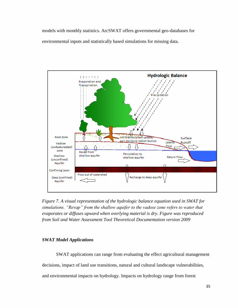
water that returns to river from the shallow aquifer layer (Arnold et al., 1998). Figure 7
visually represents all of the variables in the water balance equation used by SWAT for
simulations.
The water cycle is climate driven and requires certain environmental inputs:
precipitation, temperature, solar radiation, wind speed, and relative humidity. Data of
these inputs can be acquired from observed daily data or can be simulated in hydrologic
35
models with monthly statistics. ArcSWAT offers governmental geo-databases for
environmental inputs and statistically based simulations for missing data.
Figure 7. A visual representation of the hydrologic balance equation used in SWAT for
simulations. “Revap” from the shallow aquifer to the vadose zone refers to water that
evaporates or diffuses upward when overlying material is dry. Figure was reproduced
from Soil and Water Assessment Tool Theoretical Documentation version 2009
SWAT Model Applications
SWAT applications can range from evaluating the effect agricultural management
decisions, impact of land use transitions, natural and cultural landscape vulnerabilities,
and environmental impacts on hydrology. Impacts on hydrology range from forest

36
management, point and non-point source pollution, urbanization, and climate change. The
literature that will be discussed in the following section focuses on climate change
impacts on hydrology. The studies take place in river basins of the United States,
including the PNW, multiple river basins in Africa, and river basins in China. The
varying landscapes of the SWAT model application demonstrates the flexibility of
SWAT to be calibrated to basin specific parameters in varying terrain.
Hydrologic parameters used to simulate model output vary from study to study.
Studies that assessed climate change impacts on hydrology included hydrologic
parameters for surface flow, baseflow, and evapotranspiration (Jha et al., 2004; Stratton
et al., 2009; Sridhar & Nayak, 2010; Wu et al., 2012; Mango et al., 2011; Kanka-Yeboah
et al., 2013; Jin & Sridhar, 2012). Case studies assessing the impact of climate change on
streamflow were able to couple global climate models (GCMs) or regional climate
models (RCMs) with SWAT. Using downscaled climate models in SWAT analysis
allowed for the following investigations; future climate change scenarios impact on
annual streamflow, the relationship of projected precipitation extremes on streamflow,
future water scarcity and management adaptations, landscape adaptations for climate
change mitigation, and assessment of culturally significant areas at risk to extreme
precipitation (Jha et al., 2004; Wu et al., 2012; Mango et al., 2011; Kanka-Yeboah et al.,
2013; Jin & Sridhar, 2012). Based on the methods of these case studies, assessing climate
change impacts on streamflow in the Puyallup River basin should be applicable. The
topography and interactions of a glacier fed system could be of concern, but two case
studies in the neighboring state of Idaho were able to successfully implement SWAT in
similar landscapes (Stratton et al., 2009; Sridhar & Nayak, 2010).

37
Each case study used projected climate change scenarios and produced a level of
uncertainty for each application. Uncertainty accumulates from input data, the
downscaling of global to regional climate scenarios, and the model itself. To reduce error
and uncertainty, SWAT simulations were run with multiple climate change projections,
include more than one climate scenario, and were replicated for multiple future
timescales. The climate change impact on streamflow in two river basins of Ghana used
two climate change projections with a rapid future economic growth scenario.4
Streamflow simulations using these parameters were produced for future time periods
2020s (2006 to 2035) and 2050s (2036 to 2075) (Kanka-Yeboah et al., 2013). The two
Ghana river basin simulated streamflow reductions of 22 to 50 percent for these time
periods with future climate change scenarios. This approach implemented with SWAT
reduced uncertainty and can be reproduced in the Puyallup River basin assessment.
More influential are the Idaho case studies that were successful in implementing
SWAT in mountainous and snowpack influenced watersheds of the PNW. Sridhar and
Nayak (2010) were able to implement SWAT to assess climate variability influence on
hydrology with a 40 year data set (1967-2006). This study found that site specific
monitoring stations were key to identify natural variability of climate and climate change
impacts. Calibration of streamflow simulations at the Reynolds Mountain East weir
produced an NSE=0.90 and an R2=0.90, while validation produced an NSE=0.89 and an
R2=0.90. Streamflow peak timings showed a shifting trend of streamflow peaks occurring
8 to 10 days earlier as influence by climate warming (Sridhar & Nayak, 2010). From the
4 GCM projections were ECHAM4 (European Centre HAMburg, 4th Generation) and CSIRO
(Commonwealth Scientific and Industrial Research Organization). These projections were based off the
future emission scenario A1F1 from the IPCC AR4. The A1F1 scenario reflects a rapid future economic
growth that minimizes the economic gap between countries.

38
streamflow output statistics, model performance of the Idaho Reynolds Mountain East
weir was very good. This is significant as the PNW region experiences regional climate
variability with PDO and ENSO events which was accounted for in this Idaho case study.
The additional Idaho case study produced by Stratton et al. (2009) found similar
results with calibration statistics of NSE=0.79 and R2=0.90. In addition, Stratton et al.
(2009) recognized the importance of the sensitivity analysis to suggest significant and
sensitive parameters as well as the elevation gradient influence on model inputs. Soil
moisture output was underestimated during SWAT simulations. The underestimation
indicates the need for further detail and field observations regarding soil parameters
(available water content and saturated hydraulic conductivity), subsurface flow
parameters, and snow parameters (lapse rate and melting factors). This is important as
snowmelt and snowfall parameters are included in studies conducted in mountainous
regions with snowpack influences but are not well represented in the SWAT literature.
Though snowmelt and snowfall parameter interactions are not well discussed in the
SWAT literature, they are important and need to be included in this terrain. Combined
with downscaling and uncertainty reduction techniques in other regional studies, the
Idaho case studies suggest that SWAT can be implemented in the Puyallup River
Watershed.
Data Acquisition and Model Preparation
Use of SWAT requires data inputs of a digital elevation model (DEM), soil type
maps, land-use maps, and climatic data (Kankam-Yehoah et al., 2013; Jha, 2011; Jha et
al., 2004). The DEM, land use, and soil maps are used to divide river sub-basins into

39
smaller subdivisions, hydrologic response units (HRUs). Each subdivision consists of
similar land use types, soils, and management type. Creation of HRUs allows SWAT to
simulate hydrology variable outputs for each sub-basin before accumulation of watershed
impact (Kankam-Yeboah et al., 2013). The creation of HRUs in SWAT is critical as most
calculations are done at this spatial level.
Water storage volumes in the soil are calculated at HRU level. These water
storage profiles are snow, the soil profile (0 to 2 meters), shallow aquifer (2 to 20
meters), and deep aquifer (>20 meters) (Arnold et al., 2000; Jha et al., 2004; Jha, 2011).
The SWAT model only simulates water components in the soil profile level as the aquifer
levels are too variable for most management needs. These layers support the water
storage volumes in the form of infiltration, evaporation, plant uptake, lateral flow, and
percolation (Jha et al., 2004). Layer distinction is needed to understand the soil moisture
content and calculate evapotranspiration and ground water recharge. SWAT allows up to
10 soil layers that typically occur in the 1 to 2 meter depth range for most of the United
States (Srinivasan, 2015). These variables are important as they aid in determining total
basin yield using the water budget equation and to compute streamflow output.
Downscaling for the Pacific Northwest
The PNW is one North American region that has downscaled GCM projections.
The GCMs use annual mean temperatures as an assessment of climate change, but the
regional scale of measured temperature and precipitation can give more insight into the
effects on biological systems, including hydrology, linked to climate change
(Abatzoglou, Rupp, & Mote, 2013). Regional projections are a more accurate assessment

40
of localized impacts that local governments can use to better prepare for future risks. For
hydrology planning, policy makers do not always have the basin and sub-basin scale
information regarding climate change scenarios to adequately plan or adapt (Hamlet et
al., 2013). Having long-term assessments of climate change impacts on water resources
are essential for management strategies (Serrat-Capdevila et al., 2007). The lack of
reference information is why downscaling is significant, as the need to incorporate
climate change information into water resource planning and decision making has been
acknowledged (Hamlet and Lettenmaier, 1999; Hamlet et al., 2013).
Downscaling Climate Change Scenarios
Downscaling is used to increase the precision of modeled climate projections, but
will not necessarily increase the accuracy of the data generated. Uncertainty will
accumulate due to changing climate variables, greenhouse gas concentrations, and model
error because downscaling models increases error due to regional variability (Snover et
al., 2013). Downscaled climate scenarios will be applied in the following SWAT
analysis, as GCMs are not appropriate for PNW modeling because they do not capture
regional variability (Hamlet et al., 2013). The coarse scaled models are not designed to
take into consideration regional phenomena such as the east-west temperature and
precipitation gradients that occur in coastal mountain ranges such as the Cascade
Mountain range (Hamlet et al., 2013). Nor do the GCMs reflect seasonal variability
influenced by PDO and ENSO.

41
2.7 Conclusion
As reported by the IPCC AR5 report, new climate change scenarios indicate
warming temperature and shifting precipitation regimes for the PNW. Observations show
these shifting trends in the Puget Sound snowpack watersheds. Using hydrologic models
to incorporate future CO2 concentrations, temperature, and precipitation changes, and
assessment of climate change impacts can be simulated. These simulations can better
inform local and state agencies about future water scenarios. Having a generalized
assessment of future changes is important as the Puget Sound area supports social and
economic benefits.
The SWAT model has been successful in producing climate change impact
assessments in other river basins of the United States. The assessment of SWAT
feasibility in the Puyallup River basin will be grounded in the ability of SWAT to
successfully reproduce current and historical streamflow measurements with data inputs.
This will be addressed in the model calibration and model validation steps. The
mountainous terrain and snowpack parameters will challenge SWAT implementation in
the Puget Sound lowlands. The Puyallup River basin is glacier fed and will be impacted
by climate change as glaciers retreat and declining snowpack accumulation shifts peak
flow times. Shifting these peak flows will increase the demand for and conflict over
water resources between growing municipalities, natural resource industry demands, and
local habitats. Conducting a sub-basin and watershed scale assessment will be useful for
natural resource managers to apply adaptive management strategies to reduce future
water conflict. This research will address the feasibility of implementing the SWAT
model in the lower Puget Sound river basins.

42
Chapter 3. Methods
3.1 Study Area
The snowpack dominated Puyallup River Watershed, located in south Puget
Sound low lands of western Washington (Figure 8), and was chosen as the study site for
this thesis. The focus of the SWAT assessment was conducted in the Puyallup River
basin of the watershed, shown in Figure 9, to assess SWAT model feasibility and
parameter calibration. The Puyallup River basin drains a watershed approximately 1,040
square miles or 665,000 acres (PRWC, 2014). The watershed is fed from the glaciers on
Mt. Rainier and is drained by the Puyallup River and two main tributaries, the White
River and the Carbon River. Water supplied from the watershed is used for irrigation,
municipal, and domestic supplies. The surface water from this watershed supplies fish
habitat, recreation, and navigation while groundwater supplies public and single wells
(Washington State Department of Ecology [DOE], 1995). These rivers are home to many
endangered salmon species, supply water resources to multiple metropolises including
Tacoma, and are of cultural significance to many of the native Indian tribes including the
Puyallup Tribe of Indians.
Mean annual flows for the Puyallup River are approximately 3,000 cubic feet per
second (cfs) with peak runoff times and flooding occurring October through March
(DOE, 1995). High flows occur when the municipality supply demand is low and
conversely, low flows occur in the summer when demands rise again. USGS station
12093500 on the Puyallup River reported low flows in the summer month of August that

43
averaged 566 cfs for the years 1940 to 2000. Annual high flows for the month of
December averaged 945 cfs for the same years.
Figure 8. The Puyallup River Watershed outlined in red house portions of Mt. Rainer and
extends into the lowlands of Puget Sound located in Washington State. Upper watershed
is vastly forested and lower watershed is more urbanized.
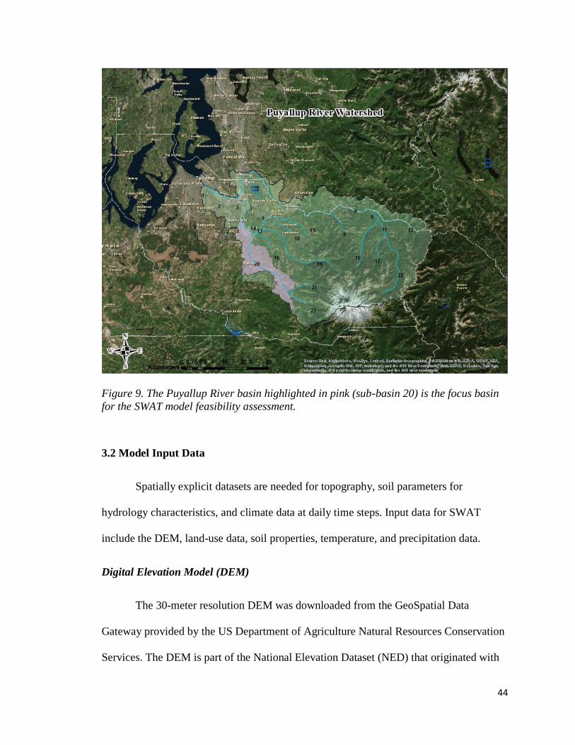
44
Figure 9. The Puyallup River basin highlighted in pink (sub-basin 20) is the focus basin
for the SWAT model feasibility assessment.
3.2 Model Input Data
Spatially explicit datasets are needed for topography, soil parameters for
hydrology characteristics, and climate data at daily time steps. Input data for SWAT
include the DEM, land-use data, soil properties, temperature, and precipitation data.
Digital Elevation Model (DEM)
The 30-meter resolution DEM was downloaded from the GeoSpatial Data
Gateway provided by the US Department of Agriculture Natural Resources Conservation
Services. The DEM is part of the National Elevation Dataset (NED) that originated with

45
the U.S. Geological Survey (USGS). NED datasets use the Nearest Neighbor resampling
method to interpolate continuous elevation data in a Universal Transverse Mercator
(UTM) projection to make seamless maps. DEM quality is of high importance as the
DEM layer sets the foundation for stream network delineation. Multiple DEM raster files
were downloaded, combined, and projected to UTM ZONE 10 N for western Washington
with datum NAD 1983. DEMs were chosen for Pierce and King Counties of Washington
State at a 30-meter resolution. Three meter and 10-meter resolutions were available but
30-meter resolution maps were chosen as seen in the SWAT literature for DEM selection.
Sub-basin delineation, shown in Figure 10, was created from the DEM layer based on
land surface and drainage patterns. Drainage patterns were used to determine flow
direction and movement.
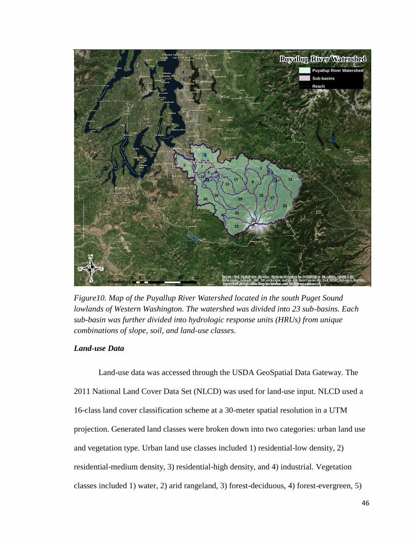
46
Figure10. Map of the Puyallup River Watershed located in the south Puget Sound
lowlands of Western Washington. The watershed was divided into 23 sub-basins. Each
sub-basin was further divided into hydrologic response units (HRUs) from unique
combinations of slope, soil, and land-use classes.
Land-use Data
Land-use data was accessed through the USDA GeoSpatial Data Gateway. The
2011 National Land Cover Data Set (NLCD) was used for land-use input. NLCD used a
16-class land cover classification scheme at a 30-meter spatial resolution in a UTM
projection. Generated land classes were broken down into two categories: urban land use
and vegetation type. Urban land use classes included 1) residential-low density, 2)
residential-medium density, 3) residential-high density, and 4) industrial. Vegetation
classes included 1) water, 2) arid rangeland, 3) forest-deciduous, 4) forest-evergreen, 5)
5
22
19
4
812
20
2
18
7
15
23
21
1716
10
914
6
11
3
1
13
Source: Esri, DigitalGlobe, GeoEye, Earthstar Geographics, CNES/Airbus DS, USDA, USGS, AEX,Getmapping, Aerogrid, IGN, IGP, swisstopo, and the GIS User Community, Esri, HERE, DeLorme, TomTom,MapmyIndia, © OpenStreetMap contributors, and the GIS user community
.
Puyallup River Watershed
Sub-basins
Reach
Puyallup River Watershed
0 10 20 30 405Kilometers

47
forest-mixed, 6) range-brush, 7) range-grasses, 8) hay, 9) agricultural land-row crops, 10)
wetlands-forested, and 11) wetlands-non-forested. The Puyallup River Watershed had a
total of 15 land-use classes for simulations.
Soil Data
Soil data were obtained from the USDA GeoSpatial Data Gateway. Soil Survey
Geographic Database (SURRGO), originated with the U.S. Department of Agriculture,
Natural Resources Conservation Service and further developed by the National
Cooperative Soil Survey (NCSS). The gridded soil layer linked soil attributes to a unique
map unit key (MUKEY) that allowed for additional county level soil surveys to be added
to the SURRGO database. Soil properties are necessary for the SWAT model as rainfall
events and destination of flow depend on the composition and conditions of the soil. Soil
properties such as texture, chemical composition, physical properties, moisture content,
hydraulic conductivity, bulk density, and organic carbon content are needed. These
properties are needed for each soil type and each soil layer as they influence the
movement of water. These properties were provided by the SURRGO database and
county level soil surveys. Deficiencies in soil survey information around Mt. Rainier in
the SURRGO database lead to areas being identified as No Digital Data in the county
level soil survey. Otherwise, soil classes for the Puyallup River Watershed can be found
in Table 2 in the Appendix. Soil grids were downloaded in NAD 1983 Albers Equal Area
Conic spatial reference and projected into UTM.

48
Climate Data
Daily observed data for precipitation (mm), minimum temperature (C°), and
maximum temperature (C°) were downloaded for Pierce County and King County of
Washington State from National Oceanic and Atmospheric Administration (NOAA)
National Climatic Data Center. Seven weather stations were chosen based on availability
of 50-year datasets, 1960 to 2010. Weather station location and averages are available in
Table 3 and Table 4. Missing data occurred for stations at various months or days and
was statistically simulated in SWAT. Other climate data simulated in SWAT included
wind speed, humidity, solar radiation, and evapotranspiration. These simulations were
based on national weather gage datasets within the SWAT model.
Streamflow Data
Daily streamflow data was obtained on the USGS website for 19 surface flow
stations throughout the Puyallup River basin. SWAT model calibration and validation
used observed streamflow data to measure simulation accuracy. The station of focus,
USGS station 12093500, was located along the Puyallup River at Orting Washington.
This station was chosen for sensitivity, calibration, and validation procedures because of
its location by the watershed outlet and complete record of historical measurements.
Streamflow measurements from 1960 to 1979 were used for calibration and streamflow
measurement from 1980 to 2007 were used for validation. Streamflow data was
normalized to the area of the drainage basin to yield units of mm/day. This was done by
converting flow from units of cubic feet per second (cfs) to millimeters per day (mm/day)
for both calibration and validation following Equation 2. Conversion to millimeters
occurred so that streamflow was more relatable to precipitation input that is also

49
measured in millimeters, but results are reported as m3/s. Figure 11 represents average
daily flow for USGS station 12093500.
(Equation 2):
Convert drainage area to square feet:
172 𝑚𝑖𝑙𝑒𝑠2 ∗27,878,400 𝑓𝑡
1 𝑚𝑖𝑙𝑒2
2
= 4,795,084,800 𝑓𝑡2
Convert cubic feet per second to cubic feet per day
1 𝑓𝑡3
1 𝑠𝑒𝑐𝑜𝑛𝑑∗
60 𝑠𝑒𝑐𝑜𝑛𝑑𝑠
1 𝑚𝑖𝑛𝑢𝑡𝑒∗
60 𝑚𝑖𝑛𝑢𝑡𝑒𝑠
1 ℎ𝑜𝑢𝑟∗
24 ℎ𝑜𝑢𝑟𝑠
1 𝑑𝑎𝑦=
86,400𝑓𝑡3
𝑑𝑎𝑦
Combine conversions
86,400𝑓𝑡3
𝑑𝑎𝑦⁄
4,795,084,800 𝑓𝑡2=
0.000189899 𝑓𝑡
𝑑𝑎𝑦
Convert to millimeters for model input
0.000189899 𝑓𝑡
𝑑𝑎𝑦∗
12 𝑖𝑛
1 𝑓𝑡∗
25.4 𝑚𝑚
1 𝑖𝑛=
0.005492 𝑚𝑚
𝑑𝑎𝑦

50
Figure 11. USGS surface water station 12093500, Puyallup River at Orting Washington.
Average daily flow (mm/day) were aggregated by month for 1960 to 2007. Observations
show two peaks, in the winter from precipitation and in the late spring from snowmelt.
Data source: USGS
3.3 SWAT Setup and Sensitivity Analysis
SWAT model setup began with delineation of the watershed based on the
obtained data. Watershed delineation included DEM setup, stream definition, outlet and
inlet definition, watershed outlet selection, and watershed outlet definition. The stream
definition was created using the DEM layer instead of burning in a stream network or
National Hydrology Dataset. This decision to use the DEM layer over predefined stream
0
1
2
3
4
5
6A
vera
ge d
aily
flo
w (
mm
/day
)
Month
Average Daily FlowUSGS Station 12093500
1960-2007
51
network was to limit sub-basin and HRU definitions. Since each reach is assigned to one
sub-basin, including all tributaries would increase the computation power needed and
error in final simulations. Using the DEM to define stream network simplified sub-basin
definition. Sub-basin outlets were defined so that each reach of a channel was assigned to
one sub-basin. With the selection of one watershed outlet, the watershed was delineated
to form 23 sub-basins (Figure 10), with the focus of assessment in sub-basin 20, the
Puyallup River basin (Figure 9).
Hydrologic response units (HRUs) were defined using land-use, soil, and slope
data grids. Rainfall and temperature input files were added to SWAT. Elevation bands
were added to SWAT input tables to account for snow accumulation of Mt. Rainier.
Elevation band ranges (meters) were adapted from Cuo et al. (2011), as follows: band 1:
0-500 m, band 2: 500-1000 m, band 3: 1000-1500 m, band 4: >1500 m.
SWAT DEM setup produced nine elevation ranges in 500 meter increments, from
sea level to 4,500 meters (Figure 12). Land-use classification resulted in fifteen classes
(Figure 13). The SURRGO database used for soil classification in SWAT resulted in 233
soil classes, 104 were listed in sub-basin 20 (Figure 14). After the three layer
classifications, 5 HRUs were derived for sub-basin 20 from unique combinations of
slope, land-use, and soil type.
After an initial SWAT simulation was conducted, sensitivity analysis was
performed to highlight basin specific parameters that drive model simulations and create
sensitivities to model outputs (Arnold et al., 2012). Highlighting sensitive parameters was

52
necessary for calibration to assess over and under estimation of output variables.5
Sensitivity analysis was conducted using SWAT-CUP and a chosen algorithm, which, for
the Puyallup River basin analysis, the Sequential Uncertainty Fitting-2 (SUFI2) algorithm
was used. SUFI2 was chosen to produce practical results as simulations are not dependent
on previous iterations (Srinivasan, 2015) and based on its use in PNW-based Idaho
watersheds (Jin & Sirdhar, 2012). Regression correlation coefficient (R2) and the Nash-
Sutcliffe model efficiency (NSE) coefficient measured how well simulated data
compared to observed data. Current literature has a range of acceptable R2 and NSE
values as reflected in Table 1 of the Appendix.
Streamflow simulations for sensitivity analysis followed Kankam-Yeboah et al.
(2013) and Jha (2011). This included a short time period of 1960 to 1965 for sensitivity
analysis and the Curve Number method (Jin & Sridhar, 2012) for surface runoff
estimation based on precipitation. Streamflow simulations were compared to observed
flow data from USGS stream gage 12093500. Simulations were opened and viewed using
SWAT-CUP for sensitivity analysis of parameters, calibration, and validation. SWAT-
CUP was designed as an interface for SWAT to link the inputs and outputs of a
calibration program to the model through text file formats.
Twenty-one parameters were observed for sensitivity analysis of streamflow
using the automated Latin Hypercube One-factor-At-a-Time (LH-OAT) sensitivity
analysis provided in SWAT-CUP snowpack dominated watershed literature from the
5 The SWAT model provides a sensitivity analysis tool that uses the Latin Hypercube One-factor-At-a-
Time (LH-OAT) method. The LH-OAT is a combination of the global sensitivity analysis method Latin
Hypercube (LH) (McKay, 1979) and the local sensitivity analysis method One-factor-At-a-Time (OAT)
(Morris, 1991) (Kankam-Yeboah et al., 2013; Mango et al., 2011). The global method allows for all
parameter values to change together and the local method changes parameter values one at a time (Arnold
et al., 2012).

53
PNW area (Sridhar & Nayka 2010, Jin & Sridhar 2012). Parameters chosen for
calibration manipulation are listed in Table 5. Using the LH-OAT analysis, a t-test was
produced to identify the significance and sensitivity of each parameter. Without expert
knowledge, a trial and error method of parameter range adjustment was used for
calibration using SWAT-CUP (Srinivasan, 2015). Expert knowledge would lead to
manual calibration of parameter ranges in the SWAT input tables (Srinivasan, 2015).

54
Parameter Parameter Name
CN2* Initial SCS runoff curve number II
CNMAX*^ Maximum canopy storage
ALPHA_BF^ Base flow alpha factor
GW_DELAY^ Groundwater delay time
GWQMN^ Threshold depth of water in shallow aquifer
for return flow
EPCO^ Plant uptake compensation factor
ESCO*^ Soil evaporation compensation factor
SOL_AWC*^ Available water capacity of the soil layer
SOL_K*^ Saturated hydraulic conductivity
RCHRG_DP*^ Deep aquifer percolation fraction
REVAPMN*^ Threshold depth of water in shallow aquifer
for percolation to deep aquifer
GW_REVAP^ Groundwater “revap” coefficient
SLSOIL*^ Slope length for lateral subsurface flow
SURLAG^ Surface runoff lag coefficient
TIMP*^ Snow pack temperature lag factor
SMFMX Melt factor for snow on June 21
SMFMN Melt factor for snow on December 21
SFTMP Snowfall temperature
SMTMP Snow melt base temperature
SNOCOVMX Minimum snow water content that
corresponds to 100% snow cover
SNO50COV Minimum snow water content that
corresponds to 50% snow cover
Table 5. Parameter and parameter description for the calibration of Puyallup River sub-
basin (sub-basin 20). (*) represents parameters that produced a positive t-Stat,
indicating sensitivity. (^) represents parameters that produced a p-value greater than
0.02, indicating significance. Snow parameters were added to calibration as suggested by
the literature.

55
3.4 Parameters
Surface Runoff
CANMX
CANMX is the maximum canopy storage (mm H2O) in the amount of water
intercepted by plant canopy. The influence of the canopy storage depends on the density
of coverage and the type of plant species. Species with greater foliage will intercept more
water and varies daily based on leaf area index. CANMX influences surface runoff,
evapotranspiration, and precipitation infiltration all of which influence total streamflow
yield. The amount of water interception at canopy level from precipitation and
evapotranspiration are considered a loss from the drainage basin. Calibration of CANMX
occurred in the default range of 0 to 100 as initial estimates began at 0, without prior
knowledge of CANMX in the Puyallup River basin, calibration adjustments started with
default range.
CN2
The initial SCS runoff curve number for moisture condition II is a function of soil
permeability, land use, and soil water condition. CN2 was developed by USDA Natural
Resources Conservation Services, also known as the Soil Conservation Service (SCS).
CN2 was chosen because it represents soil moisture conditions for average moisture
conditions (versus dry (wilting point) or wet (field capacity) conditions) and is chosen for
most modeling approaches. CN is calculated to predict runoff directly from precipitation
and is the potential of runoff from precipitation after evaporation, absorption,
transpiration, and percolation are removed. CN depends upon soil hydrologic group (A,
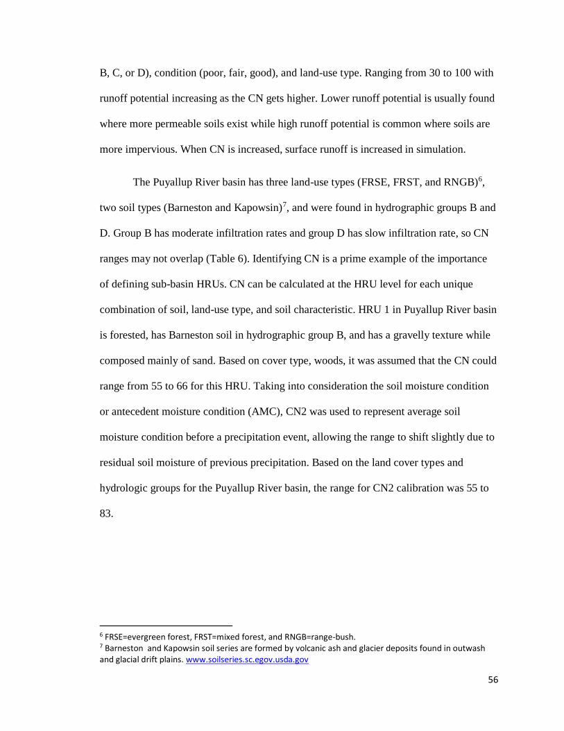
56
B, C, or D), condition (poor, fair, good), and land-use type. Ranging from 30 to 100 with
runoff potential increasing as the CN gets higher. Lower runoff potential is usually found
where more permeable soils exist while high runoff potential is common where soils are
more impervious. When CN is increased, surface runoff is increased in simulation.
The Puyallup River basin has three land-use types (FRSE, FRST, and RNGB)6,
two soil types (Barneston and Kapowsin)7, and were found in hydrographic groups B and
D. Group B has moderate infiltration rates and group D has slow infiltration rate, so CN
ranges may not overlap (Table 6). Identifying CN is a prime example of the importance
of defining sub-basin HRUs. CN can be calculated at the HRU level for each unique
combination of soil, land-use type, and soil characteristic. HRU 1 in Puyallup River basin
is forested, has Barneston soil in hydrographic group B, and has a gravelly texture while
composed mainly of sand. Based on cover type, woods, it was assumed that the CN could
range from 55 to 66 for this HRU. Taking into consideration the soil moisture condition
or antecedent moisture condition (AMC), CN2 was used to represent average soil
moisture condition before a precipitation event, allowing the range to shift slightly due to
residual soil moisture of previous precipitation. Based on the land cover types and
hydrologic groups for the Puyallup River basin, the range for CN2 calibration was 55 to
83.
6 FRSE=evergreen forest, FRST=mixed forest, and RNGB=range-bush. 7 Barneston and Kapowsin soil series are formed by volcanic ash and glacier deposits found in outwash and glacial drift plains. www.soilseries.sc.egov.usda.gov

57
Soil Hydrologic
Group
Characteristics
A High infiltration rates. Mostly sands or gravels, deep and well drained.
High rate of water transmission. Low runoff potential.
B Moderate infiltration rates. Moderately fine to coarse textures. Deep and
moderately well to well drained. Moderate rate of transmission.
C Slow infiltration rates. Moderately fine to fine texture. Slow rate of water
transmission. High runoff potential.
D Very slow infiltration rate. Moderately fine to fine texture. High
permanent water table. Clay pan or clay layer near the surface. Shallow
soils over nearly impervious material. Very slow rate of water
transmission
Table 6. Hydrologic soil groups with defining characteristics.
SOL_AWC
The available water capacity of the soil layer ( mm H2O/ mm soil), is the water
present at field capacity minus the water present at vegetation permanent wilting point,
leaving the water available for plant growth. Available water content is an indication of
soil quality and is important for vegetation growth, nutrient transport, and biological
activities. Available water capacity in this area is influenced by agricultural practices and
possible soil salt concentration if salt water intrusion occurs in the Puget Sound lowlands.
Soil texture and composition also influences available water content. Sandy soils usually
range from 25 to 100 (mm/mm), loam (silt) soil ranges from 100 to 175 (mm/mm), and
clay ranges from 175 to 250 (mm/mm) (Brouwer et al., 1985). The soil type of the
Puyallup River basin is mostly composed of sand and silt as shown in Table 7. The range

58
used for SOL_AWC calibration was 80 to110 (mm/mm) to account for the sandy like soil
type of the Puyallup River basin.
HRU Landuse
Type
Soil Type % Clay % Silt % Sand Hydrologic
Group
1 FRSE Barneston 3 30.2 66.8 B
2 FRST Kapowsin 18 38.8 43.2 D
3 FRST Kapowsin 18 38.8 43.2 D
4 RNGB Barneston 3 30.2 66.8 B
5 RNGB Barneston 3 30.2 66.8 B
Table 7. Puyallup River sub-basin (sub-basin 20) HRU description of land-use type, soil
name, and composition. FRSE=Forest-Evergreen, FRST=Forest-Mixed, RNGB=Range-
Brush.
SURLAG
The surface runoff lag coefficient accounts for surface runoff in larger basins that
does not meet the mainstem of a river on the day of generation. SURLAG controls the
fraction of runoff that is available in the main channel on any given day in relation to
time of concentration greater than a day. Time of concentration is the time required for
runoff to travel from the most distant point of an area to the outlet. As SURLAG
decreases the more water is stored in soil before it reaches the main channel. SURLAG
can be influenced by slope, land use, soil, size, and shape of the basin. SURLAG range
determination for calibration was guided by SWAT literature from other sites in the PNW
but was mostly calibrated through trial and error. Initial SURLAG estimates for the
Puyallup River basin were 2, with the full SURLAG range of 0.05 to 24 used during

59
calibration. Full range was used during calibration to account for the lack of known
SURLAG estimates in the basin.
SOL_K
The saturated hydraulic conductivity (Ksat) (mm/hr) of the soil layer is a
measurement of the ease of water to move through saturated soil. Soil property textures
influence water movement with sandy soils generally having a more rapid movement,
silts having a medium movement, and clays having a slow movement. The soil types for
the Puyallup River basin are mostly composed of sand and silt. Using saturated hydraulic
conductivity class table provided by USDA Natural Resources Conservation Service,
sandy soil Ksat Rate (µm/sec) range from 42.34 to 141.14, and silt soils Ksat Rate
(µm/sec) range from 4.23 to 14.11. After conversion, the Puyallup River basin had a
SOL_K range of 152 to 508 (mm/hr) for sandy soil and 15 to 51 (mm/hr) for silt soil
during calibration. These ranges housed initial SOL_K estimates of 32 (mm/hr) for the
silty soil type and 100 (mm/hr) for the sandy soil.
SLSOIL
SLSOIL is the slope length for lateral subsurface flow (m). Increasing slope
length can increase lateral flow in shallow subsurface layers. Lateral flow is the
movement of water from the vadose zone that enters the stream instead of percolating to
groundwater. The lateral subsurface flow is generally 5 to 20 percent of total groundwater
contribution and is dependent upon soil layer conductivity, slope, and the slope length.
Based on SWAT Check outputs before the calibration step, a number of warnings were
produced, including lateral flow being greater than the groundwater flow, and that surface

60
runoff may be too low. Slope lengths were found to be very small, at 0.5 meters; slope
length should generally be between 15 to 150 m (White et al., 2014). Short slope lengths
reduce the time and distance for water to move downslope through the soil layers before
contributing to streamflow as lateral flow. Low slope length also decreases water in the
soil layer, creating a drier soil reducing the surface runoff. SLSOIL for all HRUs in the
basin were changed to 15 meters before calibration to correct initial warnings in SWAT
Check. The range for calibration, 15 to 150 meters was chosen based on SWAT
documentation guidelines.
Base flow
ALPHA_BF
Base flow is the flow below the groundwater table that discharges to a stream and
responds to the water table and stream gradients. There must be a downhill gradient for
base flow to contribute to streamflow. If the water table is below stream level, then the
groundwater will not contribute to runoff and there will not be baseflow contribution. The
base flow alpha factor (1/days), measured as a constant, is the response of groundwater
flow to changes in streamflow recharge. The constant ranges from 0.1 to 0.3 for slow
response and 0.9 to 1.0 for quick response to recharge. Base flow alpha factor, also
known as base flow recession, depends on the topography, geology, slope, vegetation,
and drainage density of the watershed. Each of these factors will differ for each
watershed and sub-basin. Small basins with steep hillslopes, shallow soils, high drainage
density, and shallow aquifers can be expected to have small base flow recession
constants. In the Puyallup River basin, there are mixed slopes, shallow and steep, and
default values for soil depth, drainage density, and aquifer depth. From these values,

61
ALPHA_BF was underestimated and needed to be increased in calibration. The full
ALPHA_BF range, 0 to 1 was used, again due to a lacking of known observations in the
basin.
GW_DELAY
Groundwater delay time is the time it takes in days for water to percolate from the
vadose zone of the soil profile to the shallow aquifer. Properties that influence time of
water transfer are the depth of the water table and hydraulic properties of soil layers.
Within the saturated soil layers, layers with larger particle size will allow the percolation
of water more quickly leading to high conductivity. Regions of low conductivity are
layers with smaller particle size such as sand or clay, where water takes longer to move
through layers. The Puyallup River basin soil composition is mostly sand, fine particulate
size. Without knowing water table depth, low soil conductivity and basin location in the
lowlands of the watershed indicated that the groundwater delay would be large, so upper
bounds of the range were increased. Increasing GW_DELAY increases the time water
takes to enter the shallow aquifer from the soil profile, decreasing the time for the water
to contribute to streamflow.
GWQMN
The groundwater minimum depth in the shallow aquifer is the threshold (mm
H2O) that is required for base flow to return back to the reach. Base flow is the
groundwater contribution to streamflow based on water table depth. As the groundwater
minimum is increased, baseflow is decreased. The SURRGO database provided 1,000
mm H2O groundwater depth for the Puyallup River basin; however, based on the

62
differing soil types, the upper and lower bounds of the GWQMN were adjusted to find a
more accurate measurement. Based on information provided by USGS for Thurston
County groundwater station 465033122570202, groundwater depth from the 1980s to
current has ranged between 10 to 40 feet below surface (roughly 3,000 to 12,000 mm).
Thurston County is south of the study site and in the Puget Sound lowlands. No
groundwater stations were available for Pierce County or the Puyallup River Watershed.
The groundwater measurement ranges for this area, up to the 5,000 mm maximum, were
used as a starting point for range adjustments during calibration.
RCHRG_DP
Recharge depth is the deep aquifer percolation fraction. The coefficient is the
fraction of water from the root zone and shallow aquifer that percolates to the deep
aquifer. The parameter ranges from 0.0 to 1.0. Water that reaches the deep aquifer layer
is considered lost from the system; it was still calibrated for the Puyallup River basin as
water can be pulled from the deep aquifer for irrigation purposes and return to the system
later. SURRGO database defaults RCHRG_DP at 0.05, and range 0 to 1 was adjusted
based of graphical representation from simulations. Without known or observed values,
range adjustments based on simulations outputs were used.
REVAPMN
REVAPMN is the threshold depth of water in the shallow aquifer needed for
percolation (mm H2O) to occur into the deep aquifer. REVAPMN is the threshold depth
where movement from shallow aquifer to the unsaturated zone cannot occur if the
volume of the shallow aquifer is not greater or equal to REVAPMN. Increasing

63
REVAPMN changes the ease of flow of the groundwater system between layers and
increases availability of groundwater to contribute to streamflow. The range used in
calibration was the default range of 0 to 500 mm. Defaults range was used and later
adjusted based out simulation output due to lack of known or observed measurement for
the basin.
GW_REVAP
Groundwater “revap” coefficient refers to the movement of water from the
shallow aquifer to the unsaturated zone that lies above. As evaporation and root uptake
diminish water in the unsaturated zone, water is replaced by diffusion from the
underlying aquifer. The type of vegetation influences the “revap” process and are
significant in watersheds with deep-rooted vegetation. GW_REVAP ranges from 0 to 1.
As GW_REVAP approaches 0, water transmission between layers is restricted and as
GW_REVAP approaches 1, the rate of water transmission approaches the rate of
potential evapotranspiration (PET). GW_REVAP for the Puyallup River basin was
initially simulated at 0.02. A range of 0.02 to 0.2 was used for calibration as forested
vegetation in the Puyallup River basin is deep rooted and may restrict transmission.
Snow Cover/ Snow Melt
Snow fall is stored as snow pack in SWAT. Precipitation is classified as snow fall
when the average daily temperature falls below the set temperature range. When air
temperature falls below this range, any precipitation is added to snow pack and referred
to as snow water equivalent. SMFMX and SMFMN parameters impact the snow water

64
equivalent by the temperatures at which snow can fall and melt for a sub-basin. The mass
balance equation for snow pack is:
(Equation 3): 𝑆𝑁𝑂 = 𝑆𝑁𝑂 + 𝑅𝑑𝑎𝑦 − 𝐸𝑠𝑢𝑏 − 𝑆𝑁𝑂𝑚𝑙𝑡
Snow pack is the amount/depth of snow that occurs over an area. 𝑆𝑁𝑂 is the water
content of the snow pack (mm H2O) on a given day, 𝑅𝑑𝑎𝑦 is the amount of precipitation
(mm H2O), 𝐸𝑠𝑢𝑏 is the amount of sublimation (mm H2O), and 𝑆𝑁𝑂𝑚𝑙𝑡 is the amount of
snow melt (mm H2O).
SFTMP
SFTMP is snowfall temperature (°C) where the mean air temperature will allow
precipitation to fall as rain or snow/freezing rain. This temperature range should be
between -5°C and 5°C. The default for SFTMP is 1.0. If the average daily air temperature
is less than the range temperature, then precipitation for the HRU will be classified as
snow and snow precipitation is added to snow pack.
SMTMP
SMTMP is snow melt base temperature (°C) where snow pack will not melt until
snowpack threshold is met. This temperature should be between -5°C and 5°C. The
default SMTMP is 0.50; however the full range of SFTMP was used in calibration to
account for lowland temperature of snow melt, where the range is likely to be warmer for
the Puyallup River basin due to low elevation. When calibrating sub-basins at higher
elevations, such as around Mt. Rainier, this range may need further adjustment.

65
SNOCOVMX
SNOCOVMX is the minimum snow water content corresponding to 100 percent
snow cover, SNO100, (mm H2O). Snow cover will rarely be evenly distributed over an
area, often leaving exposed bare ground. Ground exposure can influence snow melt
through albedo effect. Snow water content below SNOCOVMX results in bare ground
exposure. To compute snow melt, the fraction of this bare ground to snow cover has to be
quantified. Snow cover is expressed as an aerial depletion curve where seasonal
variability of snow pack is a function of current snow pack and snow melt factor. The
depletion curve requires a snow depth threshold where there will always be 100 percent
snow cover at SNO100. Threshold depth is influenced by vegetation distribution, wind
loading, wind scouring, slope, and aspect. Ranging from 0.0 to 1.0, the smaller SNO100,
or the less water content corresponding to snow coverage, the less of an impact on snow
melt. If the water content exceeds SNO100 then the depth of the snow is considered
uniform over the area, SNO100=1.0. As SNO100 increases to 1.0, the more importance is
put on snow melt processes and the more snow cover. Depending of the percent of
SNO100, or minimum water content needed for 100 percent coverage, the volume of snow
required for full coverage varies. Usually the lower the SNO100, the smaller the volume of
snow needed for coverage. The lower the water content and volume of snow, the less
important snow melt becomes. Snow coverage will have more importance at higher
elevations and less importance at lower elevations as is the case of the Puyallup River
basin. Ranges for snow water content were chosen from literature in similar study areas
of the Pacific Northwest. Inclusion of this parameter for the Puyallup River basin could

66
be questionable, as snow melt influence surface flows, but snow cover is minimal at these
elevations.
SNO50COV
SNO50COV is the fraction of snow volume from SNOCOVMX that will be 50
percent snow cover. This fraction is assumed to be a nonlinear relationship between snow
water content and snow cover. SNO50COV is also represented by an aerial depletion
curve. Here the water content can be adjusted to find 50 percent of coverage from
SNO100. SNO50COV range varies from 0.01 to 0.99. Again, increasing snow water
content increases the volume of snow necessary to increase the fraction of aerial
coverage.
Snow melt is a linear function in SWAT calculated as the difference between
average snow pack-maximum air temperature and the threshold temperature for snow
melt. The snow melt equation:
(Equation 4): 𝑆𝑁𝑂𝑚𝑙𝑡 = 𝑏𝑚𝑙𝑡 × 𝑠𝑛𝑜𝑐𝑜𝑣 × [𝑇𝑠𝑛𝑜𝑤+𝑇𝑚𝑥
2− 𝑇𝑚𝑙𝑡]
where 𝑆𝑁𝑂𝑚𝑙𝑡 is the amount of snow melt (mm H2O) on any given day, 𝑏𝑚𝑙𝑡 is the melt
factor (mm H2O/°C-day), 𝑠𝑛𝑜𝑐𝑜𝑣 is the fraction of area covered by snow, 𝑇𝑠𝑛𝑜𝑤 is the
snow pack temperature (°C), 𝑇𝑚𝑥 is the maximum air temperature (°C), and 𝑇𝑚𝑙𝑡 is the
temperature above when snow melt occurs (°C). The 𝑏𝑚𝑙𝑡 is seasonally determined and
measured by the SMFMX and SMFMN parameters.

67
SMFMX
SMFMX is the snow melt factor on June 21st (mm H2O/°C-day). June 21st is a
standard indicator in watershed literature for the beginning of the summer season when
snow melt begins. SMFMX and SMFMN vary the amount of snow melt to occur
throughout the year and account for the impact of snow pack density on snow melt. As an
example, in rural areas, the range of snow melt factor varies from 1.4 to 6.9 mm H2O/°C-
day while the range for urban areas varies from 3.0 to 8.0 mm H2O/°C-day. The range
increases in high density areas due to snow compaction from vehicles, pedestrians, and
compaction on top of impervious surfaces such as asphalt. This parameter is not required
in the SWAT model but was included for this watershed because of the significance of
snowpack to river systems. The default of SMFMX is 4.5, but as the study site resides in
the Northern Hemisphere, where heavier snowfall occurs and so the range of SMFMX
was increased.
SMFMN
SMFMN is the snow melt factor on December 21st (mm H2O/°C-day). December
21st is a standard indicator in watershed literature for the end of summer and the
beginning of winter where snow fall starts to accumulate. Just as SMFMX above,
SMFMN accounts for the impact of snow pack density on snow melt. Together with
SMFMX, these parameters allow the rate of snow melt to vary seasonally throughout the
year as described by the snow melt equation. For rural areas, SMFMN has a range that
varies between 1.4 to 6.9 mm H2O/°C-day and a range that vary between 3.0 to 8.0 mm
H2O/°C-day for urban areas. The default of SMFMN is 4.5, but as the study site resides

68
in the Northern Hemisphere were snow fall is heavier and the range of SMFMN was
increased.
TIMP
TIMP is the snow pack temperature lag factor. This accounts for the effect of
previous day’s snow pack temperature on the present day snow pack temperature. The lag
factor accounts for snow pack density, depth, and temperature. The lag factor ranges from
0.01 to 1.0. As the factor approaches 1.0, the temperature from the previous days have
less of an impact while the present day mean air temperature has a greater effect on snow
pack temperature. The default setting for TIMP is 1.0, where previous day snow pack
temperature had less impact. The full range was used for calibration of the Puyallup
River basin to account for lack of known measurements.
Evapotranspiration
Evapotranspiration is the processes by which water on the Earth’s surface in
converted to water vapor and is the primary method that water is removed from a
watershed. It is estimated that 62 percent of all precipitation goes through
evapotranspiration and is greater than runoff in most watersheds (Dingman, 1994).
Evapotranspiration estimates are critical in understanding how climate changes, such as
increased temperature, will impact water resources. Evapotranspiration was represented
in calibration with the use of the plant compensation factor (EPCO) and the soil
evaporation compensation factor (ESCO).

69
EPCO
EPCO is the plant compensation factor. This factor is the amount of water that
vegetation will uptake that is required by the plant for evapotranspiration, which varies
daily and depends on water availability in the soil. The compensation factor ranges from
0.01 to 1.00. Depending on water availability in the layers, the closer to 1.0 the factor
reaches the more the water demand must be met by lower layers in the soil. SWAT
defaults to 1.0 for EPCO, calibration using SWAT-CUP began with range 0.01 to 1.00
and was adjusted based on simulation graphical outputs.
ESCO
ESCO is the soil evaporation compensation factor used to modify the depth of soil
layers used to meet evaporation demand. ESCO ranges from 0.01 to 1.0, as the
coefficient decreases, evaporative demand in the model can extract from lower soil
layers. ESCO was set to 0.95 from the SURGGO database, leaving only an upper range
increase of 0.05. During calibration the ESCO range was set to 0.01 to 1.0 and adjusted
based on simulation graphical output.
3.5 Calibration and Validation
Calibration and validation were done using the Sequential Uncertainty Fitting 2
(SUFI-2) algorithm as part of SWAT-CUP. Developed by Abbaspour et al. (2004, 2007),
SUFI-2 is a calibration algorithm that accounts for all sources of uncertainty in a model.
These sources include uncertainties with parameters, driving variables such as
precipitation, SWAT model execution, and observed data such as streamflow.

70
After the sensitive parameters were identified, calibration of the model aggregated
daily observations to monthly averages for the time period of 1960 to 1979 with observed
stream gage data near Orting, Washington. The 20-year time scale was chosen to account
for wet and dry years that occur as part of the PNW regional variability, which is due to
the inter-annual El Niño Southern Oscillation (ENSO) and inter-decadal Pacific Decadal
Oscillation (PDO). The data range includes part of the cool phase that began in 1947 and
ended in 1976 when a warm phase began in 1977. Monthly time steps for the years 1980
through 2007 were used for the validation of the model.
The NSE indicated how well the simulated and observed plot fit a 1:1 regression
line. Fitting a 1:1 regression line describes the power of a hydrologic model to predict
outcomes. Though there are no standardized acceptable ranges for these statistics, the
closer the values approach 1, the better the model will perform at simulating predictions
that closely match observed data.
The other measurement of simulation accuracy is the 95PPU in the graphical
representation of the simulated flows versus observed. The 95PPU stands for the 95
percent prediction uncertainty or P-factor. The 95PPU measured how well the observed
data fit into a 95 percent confidence range of uncertainty from the simulated output. R-
factor measures the range of output uncertainty represented by the visual band. A well-
calibrated model will have a small R-factor, represented as a thin 95PPU band that
houses the observed measurements.
During the calibration process, the sensitive parameters were adjusted by trial and
error to match the simulated streamflow to observed streamflow. For climate change
scenario assessments, both low and high flows need to be captured by model simulations.

71
Having a baseline of hydrology characteristics is important as future climate shifts are
expected to have drastic impacts on hydrograph peaks, future snow accumulation, and
snow melt. For validation of the model, SWAT model was run with the calibrated input
parameters. All input parameter ranges remained constant for validation of the 1980 to
2007 time series.

72
Table and Figures
Figure 12. Puyallup River Watershed elevation map (meters) generated in SWAT using digital elevation maps (DEM) retrieved from
USGS. Elevation ranges from sea level in the lower sub-basins to the top of Mt. Rainer approximately 4,800 meters (14,400 ft).
5
22
19
4
8
12
20
2
18
7
15
23
21
1716
10
9
3
14
1
6
1113
.
Puyallup River Watershed
0 4.5 9 13.5 182.25Kilometers
Mt. Rainier
Elevation (meters)
Sub-basins
Reach
Elevation
-1 - 0
1 - 500
501 - 1,000
1,001 - 1,500
1,501 - 2,000
2,001 - 2,500
2,501 - 3,000
3,001 - 3,500
3,501 - 4,000
4,001 - 4,500

73
Figure 13. Land-use classes created in SWAT using National Land-use Cover Data (NLCD) 2011 retrieved from USGS. Classes:
WATR=water, URLD= residential-low density, URMD- urban residential-medium density, URHD= residential-high density,
UIDU=industrial, SWRN= arid rangeland, FRSD= forest-deciduous, FRSE= forest-evergreen, FRST= forest-mixed, RNGB= range-
bush, RNGE= range-grasses, HAY= hay, AGRR= agricultural land-row crops, WETF= wetlands-forested, and WETN= wetlands-
non-forested.
5
22
19
12
20
4
18
8
2
15
23
21
7
1716
10
9
14
3
1
11
6
13
Puyallup River WatershedLand Use Classes
Sub-basins
Classes
WATR
URLD
URMD
URHD
UIDU
SWRN
FRSD
FRSE
FRST
RNGB
RNGE
HAY
AGRR
WETF
WETN

74
Figure 14. Soil classification created in SWAT using soil data from the Soil survey Geographic Database (SURRGO). 233 soil classes
exist and are listed in Table 2 of the Appendix. 104 soil classes are found in the Puyallup River basin. The large green soil
classification represents the portion of soil on and around Mt. Rainier that had no available digital data.
5
22
19
12
20
4
18
8
2
15
23
21
7
17 16
10
9 14
3
1
11
6
13
Puyallup River Watershed Soil Classes
Refer to Table 2 for soil class list

75
Average Precipitation (mm)
Station
ID
USGS
ID
Latitude Longitude Elevation
(m)
Annual Jan Feb Mar Apr May Jun Jul Aug Sep Oct Nov Dec
1 450945 47.17 -122.000 210 1234.6 156.7 125.1 116.2 103.3 83.9 75.3 32 42.5 64.8 109.1 176.4 153.7
2 455224 47.13 -122.267 177.1 1078.8 149.3 116 104.2 84.6 61.7 55.6 23.7 32.5 49.5 93.5 163.6 148.8
3 456803 47.20 -122.333 15.20 1043 152.4 117.3 102.7 78.1 52.5 45.9 20 29.8 45.6 91.1 160.7 151.1
4 453357 47.13 -121.633 47.45 1672.1 232.4 170.7 156.3 132.8 101.5 88.6 38.1 49.8 84.2 147.6 246.6 229.1
5 456385 46.92 -121.533 1068 1820.9 282.2 209 186.2 122.2 85 70.6 28.8 38.8 75 154.9 290.5 286.2
6 458278 47.25 -122.417 280.4 989.9 148.5 111.2 96.6 72.2 46.2 38.4 18.2 27.1 42.8 88.3 157.6 146.7
7 459171 46.90 -121.550 47.2 1888.9 291.5 215.7 192.3 127.1 90 71.8 29.6 40.8 78.3 159.9 301.3 298
Table 3. USGS weather stations. Daily precipitation (mm) observations were used as SWAT model inputs.
Average Temperature (⁰C)
Station
ID
USGS
ID
Latitude Longitude Elevation
(m)
Annual Jan Feb Mar Apr May Jun Jul Aug Sep Oct Nov Dec
1 450945 47.167 -122.000 210 Tmax 15.6 7.4 9.7 11.6 14.7 18.3 21.1 24.6 24.6 21.5 15.6 10.4 7.5
Tmin 5.1 0.5 1.3 1.9 3.6 6.3 9 10.5 10.5 8.5 5.4 2.7 0.8
2 455224 47.133 -122.267 177.1 Tmax 15.2 7 9.2 11.2 14.1 17.8 20.5 23.9 24 21 15.4 10.1 7.2
Tmin 4.9 -0 0.6 1.7 3.4 6.2 8.9 10.5 10.7 8.4 5.1 2.2 0.4
3 456803 47.2 -122.333 15.2 Tmax 16.4 8 10 12.5 15.7 19.5 22.3 25.5 25.3 22.1 16.4 11 8.1
Tmin 5.4 0.6 1.4 2.2 3.9 6.7 9.5 11 10.9 8.7 5.7 2.8 1
4 453357 47.133 -121.633 47.45 Tmax 13.1 4.1 6.5 8.6 11.9 15.9 18.9 22.6 22.5 19.7 13.8 7.5 4.3
Tmin 3.1 -2 -1 -0.3 1.5 4.4 7.3 9.1 9 6.7 3.5 0.5 -1.5
5 456385 46.917 -121.533 1068 Tmax 11.5 2.7 4.7 6.3 9.7 13.9 17.6 22 21.9 18.6 12.3 5.7 2.9
Tmin 1.5 -4 -3 -2.4 -0.4 2.5 5.6 8 8 5.6 2.1 -1.2 -3.2
6 458278 47.25 -122.417 280.4 Tmax 16.1 8.2 10 12.2 15.3 19 21.7 24.7 24.5 21.5 16.2 11.1 8.3
Tmin 6.8 1.8 2.6 3.5 5.3 8 10.7 12.4 12.5 10.5 7.3 4.2 2.2
7 459171 46.9 -121.550 47.2 Tmax 11.2 2.3 4.3 5.9 9.4 13.6 17.3 21.8 21.7 18.3 12 5.3 2.4
Tmin 1.3 -4 -3 -2.6 -0.6 2.3 5.4 7.9 7.9 5.5 2 -1.5 -3.6
Table 4. USGS weather stations. Daily temperature maximum and minimum (⁰C) were used as SWAT model inputs.

76
Chapter 4. Results
4.1 Watershed Delineation
Figures 12, 13, and 14 were produced from SWAT model setup. Figures represent digital
elevation, land-use classification, and soil classification for the watershed and Puyallup River
basin (sub-basin 20). DEM setup produced nine elevation ranges in 500 meter increments, from
sea level to 4,500 meters (Figure 12). Land-use classification resulted in fifteen classes (Figure
13). The SURRGO database used for soil classification in SWAT resulted in 233 soil classes,
104 of which were listed in the Puyallup River basin (Figure 14). After the three-layer
classifications, 5 HRUs were derived for the Puyallup River basin from unique combinations of
slope, land-use, and soil type.
4.2 Sensitivity Analysis
The LH-OAT analysis highlighted the following variables as sensitive parameters for the
watershed: initial SCS curve number for moisture condition II (CN2), maximum canopy storage
(CANMX), threshold water depth in the shallow aquifer (REVAPMN), snowpack temperature
lag factor (TIMP), slope length (SLSOIL), soil evaporation compensation factor (ESCO),
saturated hydraulic conductivity (SOL_K), available water capacity (SOL_AWC), and deep
aquifer percolation fraction (RCHRG_DP). P-values for all parameters, except CN2, were > 0.2.
Parameters with a P-value greater than 0.2 should be considered for calibration (R. Srinivasan,
personal communication, January 2015). CN2 was included in calibration, even with a p-value
less than 0.2. This decision was made because CN2 had the highest t-stat rating of all parameters,
t > 2.0. Though CN2 was not highlighted as significant for this particular sub-basin, the high
sensitivity suggests the importance of CN2 in parameter interactions. P-value and t-Stat are

77
represented in Figure 16 for each parameter. From the sensitivity analysis fifteen parameters
were highlighted for suggested use in calibration.
The literature suggests that snowfall and snow melt parameters should also be considered
for a snowpack dominated watershed. As such, a total of 21 model input parameters were chosen
for calibration based on sensitivity analysis and literature review of SWAT model applications in
snowpack dominated watersheds of the Pacific Northwest (PNW). These parameters were
broken into surface flow, baseflow, snow cover/snow melt, and evapotranspiration categories in
Table 8.
Table 9 describes the sensitive parameters and function with initial simulated SWAT
estimates, acceptable ranges for calibration, and ending calibration ranges. Initial SWAT
estimates were a result of initial simulations following data input. Acceptable ranges for
calibration were compiled from the literature and SWAT theoretical documentation. Calibration
ranges were the ranges that produced the best calibration results for this thesis based on
statistical outputs. The calibration ranges listed in the final column of Table 9 should be used
with caution as the calibration step needed to be revisited, as discussed later. The acceptable
ranges for parameters can also be relative or absolute. Relative ranges are listed as 0-1 and
represent a percentage range or adjustment, 1 to 100 percent. Absolute parameter ranges can only
be adjusted or replaced within the bounds of the range listed in Table 9.
Most initial simulation ranges fell into acceptable parameter ranges. REVAPMN was
initially simulated at 750 mm; the acceptable range was 0-500 mm. REVAPMN addresses the
availability of groundwater to contribute to streamflow by setting the threshold depth in the
shallow aquifer. In the instance of initial simulation, the shallow aquifer would have to meet a

78
minimum depth of 750 mm to contribute to streamflow. This parameter was overestimated in
initial simulation and was adjusted to occur below 100 mm for threshold depth.
Parameter Category Parameter Parameter Description
Surface Flow CANMX Maximum Canopy Storage
CN2 Curve Number for Moisture
Condition II
SOL_AWC Soil Water Capacity
SOL_K Saturated Hydraulic
Conductivity
SURLAG Surface Runoff Lag
Coefficient
SLSOIL Slope Length
Baseflow ALPHA_BF Baseflow Alpha Factor
GW_DELAY Groundwater Delay
GWQMN Threshold Water Depth in the
Shallow Aquifer
RCHRG_DP Deep Aquifer percolation
fraction
REVAPMN Threshold Water Depth in
Shallow Aquifer for “revap”
GW_REVAP Groundwater “revap”
Coefficient
Snow cover/Snow melt SFTMP Snowfall Mean Air
Temperature
SMTMP Snow Melt Mean Air
Temperature
SNOCOVMX Snow Water Equivalent for
100% Snow Cover
SNO50COV Snow Water Equivalent for
50% Snow Coverage
SMFMX Snow Melt Factor on June 21st
SMFMN Snow Melt Factor on
December 21st
TIMP Snow Pack Temperature Lag
Factor
Evapotranspiration EPCO Plant Compensation Factor
ESCO Soil Evaporation
Compensation Factor
Table 8. Twenty-one parameter and parameter descriptions used during calibration. Parameters
were divided into four categories: surface flow, baseflow, snow cover/snow melt, and
evapotranspiration.

79
Parameter Description Initial
Range
Acceptable
Range
Calibratio
n Range
CN2 Initial SCS CN II value 55-61 35-98 54.1-79.3
SOL_AWC Available water capacity (mm
H2O/mm soil)
25-250 0-1 80-110
SURLAG Surface runoff lag time (days) 2 0.05-24 10-15
SLSOIL Slope length (m) 100 0-150 50-60
CNMAX Maximum canopy storage (mm) 0 0-100 0-100
ALPHA_BF Base-flow alpha factor (days) 0.0275 0-1 0-0.5
GW_DELAY Groundwater delay (days) 31 0-500 300-350
GWQMN Threshold water depth In the shallow
aquifer for flow (mm)
1000 0-5000 400-500
RCHRG_DP Deep aquifer percolation fraction 0.05 0-1 0-0.2
REVAPMN Threshold water depth in the shallow
aquifer for "revap" (mm)
750 0-500 20-30
GW_REVAP Groundwater "revap" coefficient 0.02 0-1 0.02-0.20
EPCO Plant uptake compensation factor 1 0-1 0-0.3
ESCO Soil evaporation compensation factor 0.95 0-1 0-0.2
SMFMX Snow melt factor on June 21 (mm
H^2O/°C-day)
4.5 0-20 3-7
SMFMN Snow melt factor on December 21
(mm H^2O/°C-day)
4.5 0-20 2-5
SNOCOVMX Minimum snow water content for
100% snow cover (mm H^2O)
N/A 0-500 450-500
SNO50COV Minimum snow water content for
50% snow cover (mm H^2O)
N/A 0-1 0-1
SFTMP Snow fall base temperature (°C) 1 -20 to + 20 0-5
SMTMP Snowmelt base temperature (°C) 0.5 -20 to + 20 -5 to +5
TIMP Snowpack temperature lag factor 1 0-1 0.5-1
SOL_K Saturated hydraulic conductivity
(mm/hr)
32, 100 0-2000 30-150
Table 9. Calibration parameters for the Puyallup River basin (sub-basin 20) of the Puyallup
River Watershed. Parameter, parameter description, initial estimates, acceptable parameter
range, and ranges used in calibration are listed. Initial range estimates are a result of SWAT
model simulation from provided input data. Some initial ranges were not listed as noted by
“N/A” and were added during calibration. Ranges can be relative or absolute. Relative ranges,
represented as 0-1, result in multiplying initial values by a percent. Absolute ranges represent
value replacement between the upper and lower bounds during calibration. Most initial
simulation ranges, excluding REVAPMN, occurred in the acceptable parameter ranges.

80
4.3 Calibration/Validation
Calibration included observed streamflow measurements from the Puyallup River for the
years of 1960 to 1979, whereas validation used years 1980 to 2007. Final simulated streamflow
statistics for the Puyallup River were NSE=-0.01, R2=0.45 and NSE=0.39, R2=0.57 for
calibration and validation respectfully. The final simulation improved from the initial values of
R2=0.35 and NSE=-3.79. Both calibration and validation included all 21 parameter inputs.
Visual representation of simulated outputs for calibration and validation are represented in
Figure 17 and Figure 18. Simulations used observed streamflow measurements from the
Puyallup River at Orting, Washington.
The calibration/validation figures showed that the model did not reproduce historical data
well. Overall, streamflow was underestimated in the calibration step. Calibration especially
underestimated peak flows in the winter of 1960/61, spring of 1964, winter of 1964/65, spring
peak of 1974, and spring peak of 1975. CN2, GWQMN, ESCO, RCHRG_DP, GW_REVAP,
GW_DELAY, and SLSOIL parameter adjustments were able to produce the best calibration
results. Increasing parameter values for CN2, RCHRG_DP, GW_DELAY, and ESCO influences
simulation outputs by increasing surface runoff, increasing deep aquifer recharge, increasing the
time water resides in the soil layers before entering the shallow aquifer, and decreasing
evaporation. Decreasing GWQMN, and GW_REVAP parameter ranges influenced simulations
through increased baseflow, and increased water transfer from shallow aquifer to soil layers
allowing for an increase in baseflow. These parameter adjustments increased baseflow and total
streamflow yeild estimates. The progression of calibration trials can be seen in Figure 15. As
each set of parameters was adjusted, simulations became more accurate as described by
simulation statistics. Baseflow was not underestimated uniformly during calibration. From years

81
1960 to 1969, baseflow was more underestimated when compared to the later decade of 1970 to
1979.
Simulations using calibrated parameter ranges for validation produced more accurate
simulations. Validation simulations more closely resembled observed streamflow producing a
larger R2. Accuracy differences in simulations are likely due to more complete streamflow
readings from gaging stations in later years that were used in the validation stages and timescale
influence. The validation time series is closer to input data time series such as the land-use
change input maps. The observed streamflow values in the calibration time series had more
“extreme” peaks, many ranging between 30 to 40 m3/s. Many validation time series peaks were
below 30 m3/s and could account for the better R2 value during validation. Underestimation still
occurred in validation but simulated streamflow was closer to observed streamflow peaks.
Underestimated peaks occurred in the fall of 1980, spring of 1981, the summer melt of 1983,
spring of 1985, winter of 1990/91, winter of 1996, spring of 2001, and fall of 2004. However,
peak streamflows were simulated more accurately in the winter of 1982, winter 1984, winter of
1998, and winter of 2002.

82
Figure 15. Progression of parameter adjustments for calibration. Parameter adjustments
change simulation output, represented in red, to better represent observed streamflow,
represented in black, within the bounds of the 95PPU represented in green.

83
Figure 16. Graphical output of the global sensitivity analysis using LH-OAT provided by SWAT-CUP. Parameters are listed on the y-
axis with corresponding P-value and t-Stat on the x-axis. Larger t-Stats indicate more sensitivity. Larger P-values indicate
significance of the parameter to the system. The most sensitive parameters are CN2 (t=2.16), CANMX (t=1.24), REVAPMN (t=1.16),
TIMP (t=1.12), SLSOIL (t=0.62), ESCO (t=0.58), SOL_K (t=0.43), SOL_AWC (t=0.24), and RCHRG_DP (t=0.18). All the
parameters except CN2 had a p>0.2, a threshold for inclusion as suggested by the literature.

84
Figure 17. Parameter calibration for the Puyallup River basin of the Puyallup River Watershed, time period 1960-1979, as expanded
from Figure 15. The solid black line represents observed streamflow of the Puyallup River, red represents the simulated streamflow
after parameter adjustments, and 95PPU represents the 95% prediction uncertainty. R2= 0.45 and NSE= -0.01. Simulated streamflow
was underestimated for peak streamflows.
0
10
20
30
40
50
60
Stre
amfl
ow
(m
^3/s
)
Month-Year
Calibration (1960-1979)
95PPU
observed
Best_Sim

85
Figure 18. Parameter validation for the Puyallup River basin of the Puyallup River Watershed, time period 1980-2007. Validation
used parameter ranges from calibration. The solid black line represents observed streamflow of the Puyallup River, red represents the
simulated streamflow after parameter calibration, and 95PPU represents the 95% prediction uncertainty. R2=0.57 and NSE=0.39.
0
10
20
30
40
50
60
70
80
Jan
-80
Sep
-80
May
-81
Jan
-82
Sep
-82
May
-83
Jan
-84
Sep
-84
May
-85
Jan
-86
Sep
-86
May
-87
Jan
-88
Sep
-88
May
-89
Jan
-90
Sep
-90
May
-91
Jan
-92
Sep
-92
May
-93
Jan
-94
Sep
-94
May
-95
Jan
-96
Sep
-96
May
-97
Jan
-98
Sep
-98
May
-99
Jan
-00
Sep
-00
May
-01
Jan
-02
Sep
-02
May
-03
Jan
-04
Sep
-04
May
-05
Jan
-06
Sep
-06
May
-07
Stre
amfl
ow
(m
^3/s
)
Month-Year
Validation (1980-2007)
95PPU
observed
Best_Sim
86
Chapter 5. Discussion
Calibration/Validation
Overall, the SWAT simulations for the Puyallup River Basin did not produce
accurate streamflow output during the calibration or validation steps of the SWAT model.
Streamflow was underestimated during model calibration likely due to model
assumptions, lack of complete soil survey data, and the use of a mountainous snowpack
watershed. Historically SWAT model application has occurred in agricultural type
watersheds for management assessments. Literature was limited for SWAT applications
in snowpack dominated watersheds of the Pacific Northwest and Puget Sound region, but
SWAT was successfully implemented for two watersheds in the neighboring state of
Idaho. The Puyallup River basin results were less than satisfactory, producing R2 and
NSE statistics <0.70, in comparison to the Idaho watersheds and SWAT literature. The
unsatisfactory calibration results can be attributed to model assumptions regarding
groundwater interactions, scarce soil data, and orographic effects of a mountainous
region, particularly the windward verse leeward influence of the Cascade Mountain
range.
Idaho Watershed Comparisons
In Reynolds Creek Experimental Watershed (RCEW) Idaho, calibration and
validation of three sub-basins performed well, producing simulation statistics greater than
0.07 (Sridhar and Nayak, 2010). Table 10 displays calibration and validation statistics
for the RCEW, the Spokane River basin, and the Boise River basin of Idaho (Jin and
Sridhar, 2012). The secondary Idaho study was included to support successful SWAT

87
implementation in Washington State, as the Spokane River basin extended into the
eastern portion of Washington State. Simulations of the Spokane River basin in
Washington were able to produce acceptable calibration results, R2 and NSE values
greater than 0.07. The Spokane River basin was similar to the Puyallup River basin in
that streamflow originated from an elevation greater than 1,000 meters and settled in
lowlands less than 600 meters. The Idaho studies are important for this thesis in that the
Idaho streamflow assessments using SWAT supports the success of calibration and
validation in a snowpack dominated watersheds of the Pacific Northwest. However, it is
important to note that the Idaho watersheds occurred on the eastern side of the Cascade
Mountain range.
Orographic Effect
The Cascade Mountain range creates regional barriers between the maritime
climate along the western coast line and the drier climate on eastern leeward side of the
Cascade Mountain range. The orographic effects of the Cascades are depicted in Figure
19 and Figure 20, highlighting the contrast of precipitation rates on the western and
eastern side of the mountain range. Idaho watersheds received considerably less annual
precipitation on the eastern side of the mountain range in comparison to the Puget Sound
region on the western side of the mountain range. The dramatic contrast in monthly and
annual precipitation could have been a barrier for calibration of the SWAT model on the
western maritime side of the mountain range as the extreme seasonal precipitation events
were not well represented in simulations.

88
Though this barrier is not explicitly stated in the literature, simulations during
calibration could be impacted by influences of orographic effects on soil moisture and
baseflow contribution driven by precipitation and evaporation rates. Streamflow has been
found to be less impacted by soil moisture and baseflow contribution on the eastern side
of the Cascade Mountains due to the reduced rate of precipitation and drier climate
(Stratton et al., 2009; Jin and Sridhar, 2012). The drier climate and increased temperature
range east of the Cascades drive the evaporation rate to be more water limited than
energy limited. The water limitation factor allows for soil moisture and baseflow being
less sensitive to temperature fluctuations driven by climatic change (Tohver, Hamlet, &
Lee, 2014). The western side of the mountain range has a higher precipitation rate with
an evaporation rate that is energy limited (Tohver, Hamlet, & Lee, 2014). Therefore soil
moisture and baseflow contribution will have a larger effect on streamflow yield and
more likely to be influenced by climatic change. From these observations, the sensitive
soil moisture and baseflow components could have increased difficulty of calibration in
the Puyallup River basin because of higher precipitation events seen in a maritime
climate.
5.1 Underestimated Flow
Model Assumptions
Streamflow was underestimated in multiple trials of the Puyallup River basin
calibration process. The uneven distribution of baseflow to total streamflow yield could
be influenced by land-use change that occurred during the 1970s. Other studies have

89
found that underlying model assumptions attributed to underestimated flow outputs (Xu
et al., 2013). The SWAT water budget equation excludes water obtained in the deep
aquifer layer through percolation. For modeling purposes, exclusion of deep aquifer
water is due to the complexities of groundwater interactions. SWAT assumes water
entering the deep aquifer does not diffuse back into the shallow aquifer layer to which
water could then contribute to total streamflow yield as return flow. This assumption has
not been an issue in SWAT application literature occurring in agricultural settings, where
precipitation rates resemble those found in eastern Washington.
However, the Puyallup River basin sensitivity analysis found groundwater
parameters significant in baseflow interactions, including percolation from the deep
aquifer layer, which does not align with SWAT model assumptions. Significant baseflow
parameters include threshold water depth in the shallow aquifer for “revap”
(REVAPMN), deep aquifer percolation fraction (RCHRG_DP), groundwater “revap”
coefficient (GW_REVAP), groundwater delay time (GW_DELAY), and threshold water
depth in the shallow aquifer for flow (GWQMN). Due to SWAT model assumptions,
model simulations do not accurately represent baseflow contribution to total streamflow
during storm events (Sanadhya, Gironas, & Arabi, 2014; Ahl et al., 2008) as deep aquifer
percolation is not included in the SWAT water equation but was deemed significant in
the sensitivity analysis. Low baseflow contribution is seen in Figure 17 simulation during
winter months when storm flows are high from surface runoff. However, baseflow
contribution is low in the summer months as when baseflow contribution rate should
increase during times of low precipitation. For forested mountainous regions like the
Puget Sound lowlands, streamflow inputs typically originate from groundwater

90
contribution and lateral flow from the shallow aquifer (Bachmair and Weiler, 2011), but
this was not represented in the calibration output. Without accurate baseflow
representation, simulations are more likely to be underrepresented.
Model assumptions, sensitive groundwater parameters, and the under
representation of baseflow in the calibration output led to the use of Baseflow Filter
Program. Baseflow Filter Program, as described by Arnold et al. (1995) and Arnold et al.
(1999), estimated baseflow contribution and groundwater recharge using streamflow
records. Implementing daily streamflow data from the Puyallup River during the
calibration timescale (1960 to 1979), baseflow contribution to total streamflow for the
Puyallup River was estimated to be 66 to 76 percent for total streamflow yeild during the
calibration time period. The high contribution of baseflow and the underlying SWAT
assumptions could contribute to underestimated streamflow during calibration. Use of the
Baseflow Filter Program or an alternative like it, were not typical in the SWAT literature
and therefore not implemented in this thesis. Baseflow and groundwater contribution to a
system is based upon geographic components and climatic influences (Winter et al.,
1998). Contributions to a stream can be based on depth of aquifer layers, slope of
streambanks and underlying groundwater flow systems (Winter et al., 1998).
Contributions are also climatically driven as certain parts of a stream may only receive
groundwater contributions during low or high precipitation periods (Winter et al., 1998).
Understanding the groundwater interaction and baseflow contributions in the Puyallup
River basin would have help in estimating seasonal streamflow yields. Upon reflection,
future research should include a Baseflow Filter Program to understand the baseflow
contribution and verify the significance of groundwater parameter importance.

91
Surface flow was also underestimated during calibration as evident in the peak
flow times occurring in winter and spring months. Winter peak flows included heavy
precipitation events while spring peak flows are a combination of precipitation and spring
snowpack melt. These peaks are underestimated in SWAT simulations most likely from a
combination of factors that will be touched on here and discussed in further detail below.
These factors include low baseflow contribution assumption in the model, heavy
precipitation events that occur annually in the PNW, and the addition of spring snowmelt.
The extreme winter precipitation rates of western Washington are reflected in the
observed measurements but are not reproduced in simulation outputs. To remedy
observed and simulated streamflow yeild discrepancy, baseflow and surface flow should
be calibrated separately for snowpack dominated watersheds and areas with orographic
influences. The majority of the existing SWAT literature does not address this concept
and therefore it was not applied in this thesis but should be implemented for future
research.
Soil
Underestimated streamflow simulations also stem from the poor soil survey data
around Mt. Rainier. County level soil surveys were combined with SURGGO database to
increase coverage of the Puyallup River Watershed. Detailed soil data was missing from
a large portion of the watershed including the surrounding area of Mt. Rainier as evident
in Figure 14 where the large green soil classification around Mt. Rainier represents no
available digital data. Glacial melt and subsurface headwater interactions take place in
the data scale region and were therefore not accurately represented in the soil database as
discovered post-simulation. Capturing headwater interactions are important in the

92
Puyallup River Watershed as Puget Sound lowland headwater channels are sensitivity to
the changes in hydrology (Buffington et al., 2003) and are influenced by glacial melt and
sediment interactions. Further, the SURGGO database did not include detailed sediment
or subsurface soil properties including glacial alluvial deposits in the lowlands of Puget
Sound. Alluvial glacier deposits were not addressed as an important interaction in the
sensitivity analysis due to a lack of detailed soil data. Parameter CH_KI accounts for the
effective hydraulic conductivity of tributary channel alluvium, or the speed to which
water can move through soil layers in smaller channels of alluvial deposits. From work
produced by USGS (1998), it is known that the geologic characteristics of glacier
processes in the Puget Sound influence aquifer interactions, including alluvial deposits.
The absence of CH_KI in the sensitivity analysis suggests that the lack of detailed soil
data down plays the interaction of subsurface properties and groundwater contribution to
total streamflow.
Effects of poor detailed soil data was documented by Sanadhya, Gironas, & Arabi
(2014) in a snowpack dominated watershed of Colorado, where the lack of soil data
affected success of model calibration. The Colorado study found SOL_K, hydraulic
conductivity of soil, and ALPHA_BF, base flow recession constant, to be the most
important parameters influencing streamflow (Sanadhya, Gironas, & Arabi, 2014). The
same parameters where highlighted in the Puyallup River basin sensitivity analysis and
indicate the movement of water through the soil layers and groundwater contribution to
be significant in total streamflow for snowpack dominated systems (Sanadhya, Gironas,
& Arabi, 2014). Without detailed soil data, or with missing soil data, SOL_K initial
parameter ranges will not be accurately represented as soil layer properties and

93
characteristic determine the parameter range. Field verification may be necessary for
snowpack dominated sites as government databases are more likely to input default
values for data scarce regions, such as the area around Mt. Rainier.
Snowfall
The relationship between elevation, snow fall, snow accumulation, temperature
gradients, and snow melt in a mountainous landscape may also play a role in
underestimated streamflow during calibration. Since initial development, SWAT snowfall
and snowmelt algorithms have evolved to more accurately portray the contribution of
snow parameters to total streamflow (Fontain et al., 2002). Puyallup River basin peak
streamflow events are greatly influenced by subsurface parameters, snow parameters, and
the interaction between snow processes and groundwater. Sensitivity analysis indicated
snowmelt, groundwater recharge, and groundwater interactions as significant and
relevant processes for this snowpack dominated watershed. Other snowpack dominated
watersheds are consistent in highlighting these parameters as influential in these systems
(Sanadhya, Gironas, & Arabi, 2014; Sridhar and Nayak, 2010).
Model setup lacked detailed time series data beyond temperature and precipitation
inputs to depict snow parameters. Snow melt and snow fall was calculated in SWAT
through air temperature adjustments, but these variables are also influenced by dew point
temperature, wind movement, and solar radiation. SWAT simulated these additional
parameters, but would have benefited from observed data inputs. Snow melt factor on
June 21st, SMFMX, and snowmelt factor on December 21st, SMFMN, are two parameters
dependent on more than air temperature. Snow density and snow water content also

94
influence snow melt, but were not included as model inputs or highlighted in the initial
sensitivity analysis. Observed snowmelt and snowfall inputs are obtainable through
national snowpack telemetry stations (SNOTEL) provided by the Natural Resources
Conservation Service through the U.S. Department of Agriculture. However, these
stations were not implemented prior to 1980 and were not used during calibration or
validation. SNOTEL site 679 would be beneficial for the Puyallup River basin and is
located on Mt. Rainier at 1,564 meters (5,130 feet) elevation. SNOTEL site 679 collects
precipitation, snow depth, snow water equivalent, and temperature observations. Using
observed data from a SNOTEL site would have narrowed input ranges for snow melt and
snow cover parameters needed for SWAT simulation. Snow parameters were not
included in the initial sensitivity analysis of the Puyallup River basin because the sub-
basin outlet resided at a low elevation range. Snow parameters were included in
calibration due to headwater origins at higher elevations and as suggested by SWAT
literature. Calibration should have begun at headwater origin and progressed toward the
watershed outlet one sub-basin at a time but did not occur due to data scarcity of soil
data. For these reasons, the Puyallup River basin was chosen as an initial calibration site
to assess SWAT implementation.
Elevation bands impact snow parameters and were defined at watershed level as
suggested by Cuo et al. (2011). After further investigation, for a snowpack dominated
watershed such as the Puyallup, elevation bands should be defined at sub-basin level and
include a lapse rate calculation (Sanadhya, Gironas, & Arabi, 2014). Lapse rates
represent the temperature and precipitation gradients of increasing elevations in
mountainous regions and define the rate at which temperature decreases with increasing

95
elevation. Snowmelt and snow accumulation processes are sensitive to slight temperature
changes at higher elevations (Sanadhya, Gironas, & Arabi, 2014). The sensitivity of snow
parameters to temperature gradients warrant lapse rate at each elevation band, per sub-
basin, and should be simulated at a daily time step instead of an aggregated monthly time
step to capture climate sensitivity. Lapse rates can be determined by fitting a linear
regression model to annual precipitation and mean annual temperature against
observation station elevation. The rate of increase can then been manually incorporated
into SWAT model set up for each elevation band in each sub-basin. This was not done
for this thesis as only one study in the literature review suggested the use of an externally
generated lapse rate for elevation bands. Detailed snow parameter inputs from SNOTEL
stations and externally generated lapse rate should be included in future research for the
calibration of snow parameters.
Sensitivity Analysis Type
The parameter sensitivities found in snowpack dominated watershed heavily rely
on baseflow, subsurface, and snow processes interactions. As mentioned previously,
certain parameters were not highlighted in the Puyallup River basin sensitivity analysis.
Parameter sensitivities could have been overlooked due to lack of soil data, poor
elevation band definitions, or lack of snow processes inputs. These parameters could have
also been overlooked due to the chosen method for sensitivity analysis, the Latin-
Hypercube-One-Factor-at-a-Time (LH-OAT) analysis provided by SWAT-CUP, which
assesses the response of total streamflow to changes in various parameters.

96
The use of a variance-based global sensitivity analysis method could better
represent the parameter interactions of a snowpack dominate watershed (Sanadya,
Gionas, & Arabi, 2014) than the sensitivity analysis employed here. Sanadya, Gionas, &
Arabi (2014) found that the monthly pattern and timing of peak flows in the hydrograph
were more informative when investigating a snowpack dominated watershed than total
annual streamflow yeilds. Streamflow pattern and timing better represents snow melt and
subsurface parameter interactions due to sensitive in slight temperature and elevation
gradients. Monitoring change in timing of peak flows are better indicators of parameter
interactions than monitoring total streamflow yeild. From this observation, use of the
LH-OAT in SWAT-CUP, may have missed key parameter interactions by focusing on
total flow outputs. For a watershed with high seasonal and annual flows, when compared
to annual flows of neighboring Idaho watersheds, the extreme winter precipitation
combined with the high baseflow contribution could be viewed as outlier events in an
LH-OAT analysis. Shifting focus during the sensitivity analysis to include only months
with peak seasonal flows, such as winter and spring, could reduce the appearance of
outlier events and reveal snow parameter processes on streamflow.
Through the investigation of analysis methods, Sanadhya et al. (2014) also found
that the model output and type of statistical measurement influences the importance put
on parameter interactions. Subsurface parameter interactions had greater influence on
simulated month streamflow output when the Nash-Sutcliffe efficiency (NSE) coefficient
was used (Sanadhya et al., 2014). Snow, groundwater, and subsurface parameter
interactions had more influence on simulated monthly sreamflow outputs when
coefficient of determination (R2) and the root mean square error (RMSE) were used

97
(Sanadhya et al., 2014). Excluding NSE and incorporating RMSE as a method for
streamflow measurement would shift the focus to pattern and timing of peak flow in the
hydrograph instead of total flow output. Sanadhya et al. (2014) found this method more
effective for streamflow simulations in a snowpack dominated watershed. As a relatively
new finding, R2 and NSE were the standard in the SWAT literature and were followed in
this research; however, RMSE could be included, but should not replace NSE in future
work.
NSE assesses the predictive accuracy of model outputs to observed data. The best
calibration results from the Puyallup River basin produced an NSE of -0.01. Though
parameter ranges could have continued to be adjusted to increase NSE, an NSE less than
0 indicated that the observed mean of the calibration data (1960 to 1979) was a better
predictor of streamflow than the model simulations by incorporating peak winter flows.
NSE has been used in the hydrologic model literature to assess model simulated
streamflow compared to observed data. However, NSE is sensitive to extreme values or
outliers. The sensitivity of snowpack dominated watersheds to changes in temperature
produce extreme spring and winter streamflow peaks in a snowpack dominated system,
this is common in the PNW. Based on the nature of snowpack dominated peak timings
and the findings from Sanahya et al. (2014), using RMSE to focus of the timing and
pattern of peak flows would have better represented snowmelt processes and interactions.
Additional Influences
Upon further reflection, other challenges in the SWAT model setup could have
contributed to calibration issues. The quality of the input data, specifically precipitation

98
and measured streamflow, could influence calibration. Multiple years of precipitation
data had missing observations in some months. Missing data was simulated in SWAT
using regression analysis, as was suggested in the SWAT literature as a troubleshooting
method. Extreme winter flows could have amplified the missing observations and
accounted for some of the under representation of simulated streamflow in the early
station data for months with high seasonal flows; winters of 1960/61 and 1964/65.
Land-use data could have also accounted for calibration errors. The 2011
National Land Cover Data map used in model set up may not accurately represent land-
use classifications that occurred during the calibration time period. The Puyallup River
has been heavily influenced by irrigation practices, man-made alterations, and municipal
storage facilities post-1960s. Most notable are the Mud Mountain Dam construction in
the 1940s, logging activities from the 1940s to the 1970s, and channelization projects that
were completed in the 1970s (Kerwin, 1999). Though not suggested in the SWAT
literature, calibration time series should have used data closer to the 2011 land-use data.
Perhaps validation (1980 to 2007) and calibration (1960 to 1979) time series should have
been switched to better represent land-use impact on streamflow at the HRU level.
Though not explicitly stated, the Idaho case studies seemed to follow this logic as
calibration occurred during years 1997 to 2006 and validation time periods included years
1960 to 1979.

99
5.2 Moving Forward (Recommendations)
Had the calibration of SWAT simulations been successful for the Puyallup River
basin, climate change scenarios would have been implemented to simulate future
streamflow. Evidence provided by Mantua, Tohver, and Hamlet (2010) show that
snowpack dominated watersheds in the Puget Sound area are currently and will continue
to transition from snow to rain dominate basins. Using the variable infiltration capacity
(VIC) hydrologic model and climate change scenarios A1B8 and B19 from the
Intergovernmental Panel on Climate Change (IPCC) Fourth Assessment Report (AR4),
streamflows for the Puget Sound area will see a decrease in spring snowmelt, increase in
winter precipitation in the form of rain, and reduced summer precipitation (Mantua,
Tohver, and Hamlet, 2010; Tohver, Hamlet, & Lee, 2014). The precipitation regime
changes will increase peak streamflows in the winter and shift the spring peak snowmelt
to a few weeks earlier. These changes will be represented in the hydrograph as a
transition from a two-peaked (spring/winter) to one-peaked (winter) system. The shift in
the hydrograph will lead to an increase in winter flood events and a decrease in spring
snowmelt that normally sustains summer water demands for habitat and municipalities.
This evidence is consistent with a study conducted for the Nooksack River in the
upper Puget Sound region of Washington. The Distributed-Hydrology-Soil-Vegetation
Model (DHSVM) was implemented in this snowpack dominated system with downscaled
8 A1B scenario represents a future of rapid economic growth, a mid-century peak global population, a rapid introduction of new technologies, and a balanced reliance on multiple energy sources. Relative to 1980-1999, A1B scenario temperature range will increase 0.3⁰-0.9⁰C for years 2090-2099 (IPCC, 2007). 9 The B1 scenario represents a future with steady global population with a mid-century peak, an introduction of resource-efficient technologies, and environmental sustainability initiatives. Relative to 1980-1999, B1 scenario temperature range will increase of 1.1-2.9⁰C for years 2090-2099 (IPCC, 2007).

100
global climate models A210 and B111 from the IPCC AR4. The model simulated a future
forecast of increased winter flows, shifting of spring time snowmelt peak from decreased
snowpack accumulation, and a decrease in summer flows.
Physically based hydrologic models, such as VIC and DHSVM, are both
represented in the literature, implemented in the Pacific Northwest, and were able to
simulate future hydrology responses to changing climate. SWAT has been successful in
assessing climate change impacts on hydrology in many regions including Idaho in the
Pacific Northwest, but was not successfully calibrated in the Puyallup River basin.
DHSVM and VIC are two alternative models that could be implemented in the Puyallup
River Watershed. DHSVM was developed specifically for mountainous regions
(Wigmosta, Vail, & Lettemaier, 1994) while VIC incorporates more detailed snow
algorithms to take into consideration canopy influence on snow and new snow
accumulation as well as calibrates snow parameters separately per elevation band
(Maurer, 2011).
5.3 Conclusion
Determining hydrologic model capabilities and limitations is often difficult from
model documentation and literature. Only during application do site specific limitations
10 A2 scenario represents a heterogeneous future that is self-reliant, with an increasing population growth, and economies that develop regionally at a slower pace. Relative to 1980-1999 A2 scenario temperature range will increase 2.0-5.4⁰C for years 2090-2099 (IPCC, 2007). 11 The B1 scenario represents a future with steady global population with a mid-century peak, an introduction of resource-efficient technologies, and environmental sustainability initiatives. Relative to 1980-1999, B1 scenario temperature range will increase of 1.1-2.9⁰C for years 2090-2099 (IPCC, 2007).

101
and alternative approaches become visible. For the Puyallup River Watershed those
limitations were scarce soil data, lacking snow parameter input, model assumptions,
model output type, and analysis methods. These limitations prevented successful
calibration of the SWAT model in the Puyallup River basin. Continued research to
implement SWAT in this watershed would need to correct soil data with field
verification, include lapse rates and SNOTEL data, separate baseflow and surface flow
calibration, and define elevation bands at sub-basin level to accurately represent snow,
subsurface, and groundwater interactions. Other considerations should be made for
calibration time scale range and input data time step. Calibration time scale, or the range
of years, should still include a time set that will reflect regional dry and wet years as it
did in this research but the time scale should be closer in range to other input data dates
such as the recent 2011 National Land Cover data.
Time step for calibration should also be carefully chosen. Daily observations were
aggregated into monthly observations for calibration input, but should be left at daily
time step with focus on months with peak flows versus annual flows. This will shift the
focus to pattern and timing of streamflow versus total annual streamflow yield. This
option is more suitable in a region that has extreme seasonal precipitation events like the
Puyallup River Watershed. For immediate implementation of hydrologic modeling in the
PNW, VIC or DHSVM would be preferred models, as they have been developed to
specifically represent mountainous ranges and snow parameter interactions in PNW
region.

102
Tables and Figures
Table 10. RME=Reynolds Mountain East. (*)= sub-basin located in the Reynolds Creek
Experimental Watershed in Idaho. (**)=sub-basin located in Boise River basin, Idaho.
(***)=sub-basin located in Spokane River basin, Idaho. (****)=sub-basin located in
Spokane River basin, Washington.
Sub-basin Time period Simulation R2 NSE
Puyallup River 1960-1979 Calibration 0.45 -0.01
1980-2007 Validation 0.57 0.39
RME* 1997-2006 Calibration 0.9 0.9
1967-1996 Validation 0.89 0.89
Tollgate* 1997-2006 Calibration 0.87 0.84
1967-1996 Validation 0.85 0.82
Outlet* 1997-2006 Calibration 0.82 0.7
1967-1996 Validation 0.71 0.68
Parma** 1959-1963 Calibration 0.8 0.73
1964-2004 Validation 0.82 0.79
Arrowrock** 1959-1963 Calibration 0.75 0.75
1964-2004 Validation 0.77 0.7
Post Falls*** 1978-1980 Calibration 0.76 0.58
1953-1977 Validation 0.72 0.65
Spokane**** 1978-1980 Calibration 0.75 0.55
1953-1977 Validation 0.71 0.62
1981-1999 Validation 0.66 0.41

103
Figure 19. Average annual precipitation (cm) of 1961-1990 for the Pacific Northwest:
Washington, Oregon, Idaho, and western Montana. The map showcases a wetter climate
west of the Cascade Mountain range, the windward that extends the coast of Washington
and Oregon. The eastern side has a drier climate. The Puget Sound lowlands west of the
Cascade Mountain range receive more annual precipitation than the watersheds of
Idaho. Difference of annual precipitation ranges can influence the ease of SWAT model
calibration when using total streamflow yield as an output and calculating snow
parameters due to mountain range effects on climate. Figure retrieved April 2015 from
Climate Impacts Group, University of Washington.

104
Figure 20. Average monthly precipitation (mm) for the Pacific Northwest from 1900-
1998. The western side of the Cascade Mountain range receives more precipitation than
eastern side of the Cascades all year round. The greatest difference of precipitation
occurs in the winter months. Figure retrieved April 2015 from Climate Impacts Group,
University of Washington.

105
Bibliography
Abatzoglou, J.T., and Brown, T.J. (2011). A comparison of statistical downscaling
methods suited for wildfire applications. International Journal of Climatology, 32(5),
772-780.
Abatzoglou, J.T., Rupp, D.E., & Mote, P.W. (2013). Seasonal climate variability and
change in the Pacific Northwest of the United States. American Meteorological Society,
27, 2125-2142.
Abbaspour, K.C., Johnson, C.A., & van Genuchten, M.T. (2004). Estimating uncertain
flow and transport parameters using sequential uncertainty fitting procedure. Vadose
Zone Journal, 3(4), 1340-1352.
Abbaspour, K.C., Yang, J., Maximov, I., Siber, R., Bogner, K., Mieleitner, J., Zobrist, J.,
& Srinivasan, R. (2007). Modelling hydrology and water quality in the pre-alpine/alpine
Thur watershed using SWAT. Journal of Hydrology, 333, 413-430.
Ahl, R.S., Woods, S.W., & Zuuring, H.R. (2008). Hydrologic calibration and validation
of SWAT in a snow-dominated rocky mountain watershed, Montana, U.S.A. Journal of
the American Water Resources Association 44(6), 1411-1430.
Arnold, J.G. and Allen, P.M. (1999). Automated methods for estimating baseflow and
ground water recharge from streamflow records. Journal of the American Water
Resources Association, 35(2): 411-424.
Arnold, J.G., Allen, P.M., Muttiah, R., and Bernhardt, G. (1995). Automated base flow
separation and recession analysis techniques. Ground Water, 33(6): 1010-1018.
Arnold, J.G., Moriasi, D.N., Gassman, P.W., Abbaspour, K.C., White, M.J., Srinivasan,
R,Santhi, C., ….& Jha, M.K. (2012). SWAT: Model use, calibration, and validation.
Transactions of the ASABE, 55(4), 1491-1508.
Arnold, J.G., Muttiah, R.S., Srinivasan, R., & Allen, P.M. (2000). Regional estimation of
base flow and groundwater recharge in the upper Mississippi river basin. Journal of
Hydrology, 227, 21-40.
Arnold, J.G., Srinivasan, R., Muttiah, R.S., & Williams, J.R. (1998). Large area
hydrologic modeling and assessment part I: Model development. Journal of the American
Water Resources Association, 34(1), 73-89.
Bachmair, S., & Weiler, M. (2011). New dimensions of hillslope hydrology. Forest
hydrology and biogeochemistry, 216: 455-481.

106
Brouwer, C., Goffeau, A., & Heibloem, M. 1985. Irrigation Water Management: Training
Manual No. 1. Introduction to Irrigation. Food and Agriculture Organization of the
United States.
Buffington, J.M., Woodsmith, R.D., Booth, D.B., Montgomery, D.R., and Wall, L.
(2003). Fluvial processes in Puget Sound rivers and the Pacific Northwest. Seattle,
Washington: University of Washington Press.
Climate Impacts Group, University of Washington. (2013). State of Knowledge Report.
Climate.
Climate Impacts Group. (n.d.). Retrieved November 28, 2014, from
http://cses.washington.edu/cig/
Cuo, L., Beyene, T.K., Voisin, N., Su, F., Letternmaier, D.P., Alberti, M., & Richey, J.E.
(2011). Effects of mid-twenty-first century climate and land cover change on the
hydrology of the Puget Sound basin, Washington. Hydrological Processes, 25, 1729-
1753.
Dickerson-Lange, S.E., and Mitchel, R. (2014). Modeling the effects of climate change
projections on streamflow in the Nooksack River basin, Northwest Washington.
Hydrological Processes, 28, 5236-5250.
Dingman, S.L. (1994). Physical Hydrology, MacMillan Publishing Company, New York.
Duan, Q., Gupta, V.K. and Sorooshian, S. (1992). Effective and efficient global
optimization for conceptual rainfall-runoff models. Water Resource Research, 28, 1015-
1031.
Elsner, M.M., Cuo, L., Voisin, N., Deems, J.S., Hamlet, A.F., Vano, J.A., Mickelson,
K.E.B., Lee, S., Lettenmaier, D.P., (2010). Implications of 21st century climate change
for the hydrology of Washington State. Climatic Change, 225-260.
Fontaine, T.A., Cruickshank, T.S., Arnold, J.G., & Hotchkiss, R.H. (2002). Development
of a snowfall-snowmelt routine for mountainous terrain for the soil water assessment tool
(SWAT). Journal of Hydrology, 262, 209-223.
Fountain, A.G., Hoffman, M., Jackson, K., Basagic, H., Nylen, T., & Percy, D. 2007.
Digital outlines and topography of the glaciers of the American West. U.S. Geological
Survey Open-File Report 2006-1340, 23pgs.
Fritze, H., Stewart, I.T., & Pebesma, E.J. (2011). Shifts in western North American
snowmelt runoff regimes for the recent warm decades. Journal of Hydrometerology, 12,
989-1006.

107
Gassman, P.W., Reyes, M., Green, C.H., & Arnold, J.G. (2007). The Soil and Water
Assessment Tool: Historical development, applications, and future directions.
Transactions of the American Society of Agricultural and Biological Engineers, 50(4),
1211-1250.
Grimm, N.B., Chapin III, F.S., Bierwagen, B., Gonzalez, P., Groffman, P.M. Luo, Y.,
Melton, F., ….& Williamson, C.E. (2013). The impacts of climate change on ecosystem
structure and function. Frontiers in Ecology and the Environment, 11(9), 474-482.
Haak, A.L., Williams, J.E., Isaak, D., Todd, A., Muhlfeld, C.C., Kershner, J.L.,
Gresswell, R.E., Hostetler, S.W., and Neville, H.M. (2010). The potential influence of
change climate on the persistence of salmonids of the inland west. U.S. Geological
Survey Open-File Report 2010-1236, 74p.
Hamlet, A.F. (2011). Assessing water resources adaptive capacity to climate change
impacts in the Pacific Northwest region of North America. Hydrology and Earth System
Science, 15, 1427-1443.
Hamlet, A.F., Elsner, M.M. Mauger, G.S., Lee, S-Y., Tohver, I., & Norheim, R.A.
(2013). An overview of the Columbia Basin Climate Change Scenarios Project:
Approach, methods, and summary of key results. Atmosphere-Ocean, 51(4), 392-415.
Hamlet, A.F., and Lettenmaier, D.P. (1999). Effects of climate change on hydrology and
water resources in the Columbia River Basin. Journal of the American Water Resources
Association, 35(6), 1597-1623.
Hamlet, A.F., and Lettenmaier, D.P. (2005). Production of temporally consistent gridded
precipitation and temperature fields for the continental United States. Journal of
Hydrometeorology, 6(3), 330-336.
Hamlet, A.F., Mote, P.W., Clark, M.P., & Lettenmaier, D.P. (2005b). Effects of
temperature and precipitation variability on snowpack trends in the western United
States. Journal of Climate, 18(21), 4545-4561.
Harmel, R.D., Smith, P.K., Migliaccio, K.W., Chaubey, I., Douglas-Mankin, K.R.,
Benham, B., Shukla, S., Munoz-Carpena, R., & Robson, B.J. (2014). Evaluating,
interpreting, and communicating performance of hydrologic/water quality models
considering intended use: A review and recommendations. Environmental Modelling &
Software, 57, 40-51.
Hekkers, ML. (2008). Climatic and spatial variation of Mount Rainier’s glaciers for the
last 12,000 years, Washington, U.S.A. (Master’s Thesis). Portland State University.
Portland, Oregon.

108
IPCC, 2007: Summary for Policymakers. In: Climate Change 2007: The Physical Science
Basis. Contribution of Working Group I to the Fourth Assessment Report of the
Intergovernmental Panel on Climate Change. Solomon, S., Qin, D., Manning, M., Chen,
Z., Marquis, M., Averyt, K.B., Tignor, M., & Miller, H.L. (eds.) Cambridge University
Press, Cambridge, United Kingdom and New York, NY, USA.
IPCC, 2013: Climate Change 2013: The Physical Science Basis. Contribution of Working
Group I to the Fifth Assessment Report of the Intergovernmental Panel on Climate
Change [Stocker, T.F., D. Qin, G.-K. Plattner, M. Tignor, S.K. Allen, J. Boschung, A.
Nauels, Y. Xia, V. Bex and P.M. Midgley (eds.)]. Cambridge University Press,
Cambridge, United Kingdom and New York, NY, USA.
IPCC, 2014: Climate Change 2014: Impacts, Adaptation, and Vulnerability. Part A:
Global and Sectoral Aspects. Contribution of Working Group II to the Fifth Assessment
Report of the Intergovernmental Panel on Climate Change. [Field, C.B., V.R. Barros,
D.J. Dokken, K.J. Mach, M.D. Mastrandrea, T.E. Bilir, M. Chatterjee, K.L. Ebi, Y.O.
Estrada, R.C. Genova, B. Girma, E.S. Kissel, A.N. Levy, S. MacCracken, P.R.
Mastrandrea, and L.L.White (eds.)]. Cambridge University Press, Cambridge, United
Kingdom and New York, NY, USA
Isaak, D.J., Wollrab, S., Horan, D., & Chandler, G. (2010). Climate change effects on
stream and river temperatures across the northwest U.S. from 1980-2009 and
implications for salmonid fishes. Climatic Change, 113, 499-524.
Jha, M.K. (2011). Evaluating hydrologic response of an agricultural watershed for
watershed analysis. Water, 3, 604-617.
Jha, M.K., Pan, Z., Takle, E.S., & Gu, R. (2004). Impacts of climate change on
streamflow in the upper Mississippi River basin: A regional climate model perspective.
Journal of Geophysical Research, 109, D09105.
Jha, M.K. and Gassman, P.W., (2014). Changes in hydrology and streamflow as
predicted by a modelling experiment forced with climate models. Hydrological
Processes, 28, 2772-2781.
Jin, X., and Sridhar, V. (2012). Impacts of climate change on hydrology and water
resources in the Boise and Spokane River basins. Journal of the American Water
Resources Association, 48(2), 197-220.
Kankam-Yeboah, K., Obuobie, E., Amisigo, B., & Opoku-Ankomah, Y. (2013). Impact
of climate change on streamflow in selected river basins in Ghana. Hydrological Sciences
Journal, 58(4), 773-788.
109
Kerwin, J. (1999). Salmon and Steelhead Habitat Limiting Factors. Water Resource
Inventory Area, 11.
Ko, G.W., Dineshram, R., Campanati, C., Chang, V.B., Havenhand, J., & Thiyagarajan,
V. (2014). Interactive effects of ocean acidification, elevated temperature, and reduced
salinity on early-life stages of the pacific oyster. Environmental Science & Technology,
48(17), 10079-10188.
Lutz, E.R., Hamlet, A.F., and Littell, J.S. 2012. Paleoreconstruction of cool season
precipitation and warm season streamflow in the Pacific Northwest with applications to
climate change assessment. Water Resources Research, 48(1), 1525-1541.
MACA's Webpage. (n.d.). Retrieved November 29, 2014, from
http://maca.northwestknowledge.net/
Mango, L.M., Melesse, A.M., McClain, M.E., Gann, D., & Setegn, S.G. (2011). Land use
and climate change impacts on the hydrology of the upper Mara River basin, Kenya:
results of a modeling study to support better resource management. Hydrology and Earth
System Sciences, 15, 2245-2258.
Mantua, N., Tohver, I., and Hamlet, A. (2010). Climate change impacts on streamflow
extremes and summertime stream temperature and their possible consequences for
freshwater salmon habitat in Washington State. Climatic Change, 102, 187-223.
Maurer, E. (2011) VIC Hydrology Model Training Workshop-Part I: About the VIC
model [PDF document]. Retrieved from Lecture Notes Online Website:
www.engr.scu.edu/~emaurer/chile/vic_taller/01_vic_training_overview_processes.pdf
McKay, M.D., Beckman, R.J., Conover, W.J., (1979). A comparison of three methods for
selecting values of input variables in the analysis of output from a computer code.
Technometrics, 21 (2), 239– 245.
Monteith, J.L. (1965). Evaporation and environment. Symposia of the Society for
Experimental Biology, 19, No. 205-23.
Moriasi, D.N., Wilson, B.N., Douglas-Mankin, K.R., Arnold, J.G., & Gowda, P.H.
(2012). Hydrologic and water quality models: Use, calibration, and validation.
Transactions of the American Society of Agricultural and Biological Engineers, 55(4),
1241-1247.
Morris, M.D., 1991. Factorial sampling plans for preliminary computational experiments.
Technometrics, 33, nr2.
Morrison, J., Quick, M.C., Foreman, M.G.G. (2002). Climate change in the Fraser River
watershed: flow and temperature projections. Journal of Hydrology, 263, 230-244.

110
Mote, P.W. (2003). Trends in temperature and precipitation in the Pacific Northwest.
Northwest Science, 77, 271-282.
Mote, P.W. (2006). Climate-driven variability and trends in mountain snowpack in
western North America. American Meteorological Society, 19, 6209-6220.
Mote, P.W. and Salathe Jr., E.P. (2010). Future climate in the Pacific Northwest. Climatic
Change, 22p.
National Climate Change Viewer (NCCV) Home. (n.d.). Retrieved November 29, 2014,
from http://www.usgs.gov/climate_landuse/clu_rd/nccv.asp
Mote, P. W., Snover, A. K., Capalbo, S., Eigenbrode, S.D., Glick, P., Littell, J.,
Raymondi, R., and Reeder, S., (2014). Chapter 21: Northwest. Climate Change Impacts
in the United States: Third National Climate Assessment, Melillo, J.M., Richmond, T.,
and Yohe, G.W., Eds., U.S. Global Change Research Program, 487-513.
Nylen, TH. (2004). Spatial and temporal variation of glaciers (1913-1994) on Mt. Rainier
and the relation with climate. (Master’s Thesis). Portland State University. Portland,
Oregon.
Patte, D. [Eds. Abatzoglou, J., Hegewisch, K., & Hostetler, S]. (2014). Climate trends
and projections-A guide to information and references. Received in email from Climate
Impacts Group, November 2014.
Pielke, R.A., and Wilby, R.L. (2012). Regional climate downscaling: What's the point?
Eos, Transactions American Geophysical Union, 93(5), 52-53.
Polebitski, A.S., Palmer, R.N., & Waddell, P. (2011). Evaluating water demands under
climate change and transitions in the urban environment. Journal of Water Resources
Planning and Management, 249-257.
PRWC. Puyallup River Watershed Council. February (2014). Puyallup River Watershed
Assessment (DRAFT).
Puget Sound Regional Council. (n. d.) Puget Sound Regional Trends. (2006). Retrieved
November 29, 2014, from http://www.psrc.org/data/trends
Puyallup River Watershed Council [PRWC]. February 2014. Puyallup River Watershed
Assessment (DRAFT)
Romero-Lankao, P., Gurney, K.R., Seto, K.C., Chester, M., Duren, R.M. …& Stokes, E.
(2014). A critical knowledge pathway to low-carbon, sustainable futures: Integrated
understanding of urbanization, urban areas, and carbon. Earth’s Future, 2(10), 515-532.

111
Rosenberg, E.A., Keys, P.W., Booth, D.B., Hartley, D., Burkey, J., Steinemann, A.C., &
Lettenmaier, D.P. (2010). Precipitation extremes and the impacts of climate change on
stormwater infrastructure in Washington State. Climatic Change, 102(1-2), 319-349.
Salathe, E.P., Mote, P.W., and Wiley, M.W. (2007). Review of scenario selection and
downscaling methods for the assessment of climate change impacts on hydrology in
the United States Pacific Northwest. International Journal of Climatology, 27, 1611-
1621.
Sanadhya, P., Gironas, J., & Arabi, M. (2014). Global sensitivity analysis of hydrologic
processes in major snow-dominated mountainous river basins in Colorado. Hydrological
Processes, 28, 3404-3418.
Serrat-Capdevila, A., Valdes, J. B., Perez, J. G., Baird, K., Mata, L. J., & Maddock III, T.
(2007). Modeling climate change impacts –and uncertainty- on the hydrology of a
riparian system: The San Pedro Basin (Arizona/Sonora). Journal of Hydrology, 347, 48-
66.
Setegn, S.G., Srinivasan, R., Melesse, A.M., & Dargahi, B. (2010). SWAT model
application and prediction uncertainty analysis in the Lake Tana basin, Ethiopia.
Hydrological Processes, 24, 357-367.
Snover, A.K., Mantua, N.J., Littell, J.S. Alexander, M.A., Mcclure, M.M., & Nye, J.
(2013). Choosing and using climate-change scenarios for ecological-impact assessments
and conservation decisions. Conservation Biology, 27(6), 1147-1157.
Snover, A.K., Mauger, G.S., Whitely Binder, L.C., Krosby, M. & Tohver, I. (2013b).
Climate Change Impacts and Adaptation in Washington State: Technical Summaries for
Decision Makers. State of Knowledge Report prepared for the Washington State
Department of Ecology. Climate Impacts Group, University of Washington, Seattle.
Sridhar, V. and Nayak, A. (2010). Implications of climate-driven variability and trends
for the hydrologic assessment of the Reynolds Creek Experimental Watershed, Idaho.
Journal of Hydrology. 385, 183-202.
Srinivasan, R. (2015). Soil and Water Assessment Tool Beginner SWAT Training
Manual. Workshop at Spatial Science Laboratory, Texas A&M University. January 26-
28th 2015.
Stone, M.C., Hotchkiss, R.H., Hubbard, C.M., Fontain, T.A., Merans, L.O., Arnold, J.G.
(2001). Impacts of climate change on Missouri River basin water yield. Journal of
American Water Resources Association, 37, 1119-1130.
SWAT2012 Input/Output File Documentation. (n.d.) Retrieved from
http://swat.tamu.edu/documentation/ November 29, 2014.

112
Tohver, I.M., Hamlet, A.F., & Lee, S. (2014). Impacts of 21st-century climate change on
hydrologic extremes in the Pacific Northwest Region of North America. Journal of the
American Water Resources Association, 50(6), 1461-1476.
Traynham, L., Palmer, R. & Polebitski, A. (2011). Impacts of future climate conditions
and forecasted population growth on water supply systems in the Puget Sound region.
Journal of Water Resource Planning and Management, 318-326.
United States Fish and Wildlife Service Pacific Region, Science Applications. (2014).
Climate trends and projections-A guide to information and references. Patte, D. [Editors:
Abatzoglou, J., Hegewisch, K., & Gostetler, S.] pp.1-8.
United States Geological Survey. (1998). Hydrogeologic framework of the Puget Sound
aquifer system, Washington and British Columbia. Regional aquifer-system analysis-
Puget- Willamette lowland. (USGS Professional Paper 1424-D). Washington, DC: U.S.
Government Printing Office.
United States Government. (1988). Endangered Species Act of 1973, as amended through
the 100th Congress. U.S. Department of the Interior. Title 16 United States Code, 1531-
1544. Print.
van Griensven, A., and Meixner, T. (2006). Methods to quantify and identify the sources
of uncertainty or river basin water quality models. Water Science Technology, 53(1), 51-
59.
Vano, J.A., Voisin, N., Cuo, L., Hamlet, A.F., Elsner, M.M., Palmer, R.N.,... &
Lettenmaier, D.P. (2010). Climate change impacts on water management in the Puget
Sound region, Washington State, USA. Climatic Change, 102(1-2), 261-286.
Washington State Department of Ecology. (1995). Puyallup-White Watershed initial
assessment. (DOE Publication No. 95-156).
Washington State Department of Ecology. (2012). Focus on Water Availability:
Puyallup-White Watershed, WRIA 10. (DOE Water Resources Program Publication No.
11-11-015).
Washington State Department of Ecology. Water Resources Program. January 1995.
Puyallup-White Watershed assessment summary. Pub. No. 95-156 pp.1-8.
White, M.J., Harmel, R.D., Arnold, J.G., & Williams, J.R. (2014). SWAT Check: A
screening tool to assist users in the identification of potential model application problems.
Journal of Environmental Quality, 43, 208-214.

113
Wiley, M.W. and Palmer, R.N. (2008). Estimating the impacts and uncertainty of climate
change on a municipal water supply system. Journal of Water Resources Planning and
Management, 134(3), 239-246.
Winter, T.C., Harvey, J.W., Franke, O.L., & Alley, W.M. (1998). Ground water and
surface water: a single resource. U.S. Geological Survey circular: 1139. Library of
Congress, Denver, Colorado, USA.
Wu, Y., Lin, S., Abdul-Aziz, O.I. (2012). Hydrological effects of the increased CO2 and
climate change in the upper Mississippi River basin using a modified SWAT. Climatic
Change, 110, 977-1003.
Xu, P., Zhang, X., Ran, Q., & Tian, Y. (2013). Impact of climate change on hydrology of
upper reaches of Qiantang River basin, East China. Journal of Hydrology, 483, 51-60.
Zahabiyoun, B., Goodarzi, M.R., Massah Bavani, A.R., & Azamathulla, H.M. (2013).
Assessment of climate change impact on the Gharesou River basin using SWAT
hydrological model. Clean-Soil, Air, Water, 41(6), 601-609.
Zhang, X., Xu, Y., & Fu, G. (2014). Uncertainties in SWAT extreme flow simulation
under climate change. Journal of Hydrology, 515, 205-222.
Zhou, Z., Xie, S., Zheng, X., Liu, Q., & Wang, H. (2014). Global warming-induced
changes in El Niño teleconnections over the North Pacific and North America. Journal of
Climate, 27. 9050-9064.

114
Appendices
Table 1. A consolidation of referenced literature to portray the variation of sensitivity
tools, sensitive parameters, calibration/validation statistics, time scales, and error
statistics. Parameter definitions are as follows: ALPHA_BF=Baseflow alpha factor,
BIOMIX=biological mixing efficiency, BLAI=maximum potential leaf area index,
CANMX=maximum canopy storage, CH_K2=effective hydraulic conductivity,
CH_N=Manning’s n value, CN=runoff curve number, CN2=initial SCS runoff curve
number, EPCO=plant uptake compensation factor, ESCO=soil evaporation
compensation factor, GW_DELAY=groundwater delay time, GW_REVAP= ground water
“revap” coefficient, GWQMN= threshold depth of water in shallow aquifer required for
return flow, RECHRG_DP=deep aquifer percolation fraction, REVAPMN=threshold
depth of water in shallow aquifer for percolation, SMFMN=melt factor for snow on
December 21, SMTMP=snow melt base temperature, SOL_ALB=moist soil albedo,
SOL_AWC=available water capacity of soil layer, SOL_K=saturated hydraulic
conductivity, SOL_Z=depth from soil surface to bottom of layer, SPCO=maximum
amount of sediment that can be transported, and SURLAG=surface runoff lag coefficient.
In depth definition can be found in SWAT2012 Input/Output File Documentation at
(swat.tamu.edu/documentation/).
Paper Sensitivity
Analysis
Sensitive
Parameters
Calibration Validation Error
Analysis
SWAT
simulatio
n ability
Arnold
et al.,
2000
Referenced CN
ESCO
SOL_AWC
1960-1980
R2=0.89
(average annual
flow)
1981-1985
R2=0.65
(monthly
stream
flow)
In agreement with
two other base
flow models
Jha et
al.,
2004
Streamflow 1989-1997
Annual
R2= 0.91;
NSE=0.91
Monthly
R2= 0.75;
NSE=0.67
1980-1988
Annual
R2= 0.89;
NSE=0.86
Monthly
R2= 0.70;
NSE=0.59
BIAS
RMSE
Was able to
produce stream
flows with
reasonable
accuracy
Jha
2011
Influence
coefficient
method
CN
ESCO
SOL_AWC
1988-1993
Monthly flows
R2= 0.86;
NSE=0.85
1982-1987
Monthly
flows
R2= 0.69;
NSE=0.61
Strong correlation
found between
predicted and
simulated flows
Mango
et al.,
2011
ParaSol
SUFI-2
ESCO
CN2
ALPHA_BF
GWQMN
SOL_Z
REVAPMN
SOL_AWC
CH_K2
Rain gauge
data
1996-2003
for calibration
R2= 0.09;
NSE=-0.53
RFE data
Rain gauge
data
1996-2003
for
validation
R2= 0.32;
NSE=-0.06
Correlation
between
simulations and
rain gauge data
were poor.
Simulated data
with infrared
Rainfall Estimated

115
BLAI
CANMX
2002-2005
for calibration
R2= 0.56;
NSE=0.43
RFE data
2002-2005
for
validation
R2= 0.43;
NSE=0.23
(RFE) were fair.
Kanka
m-
Yeboah
et al.,
2013
LH-OAT CN
ESCO
EPCO
SOL_AWC
GW_REVAP
GW_DELAY
RECHRG_D
P
GWQMN
ALPHA_BF
SOL_Z
REVAPMN
SOL_K
SOL_ALB
White Volta
1983-1993
R2= 0.76;
NSE=0.76;
PBIAS(%)=-
1.5
Pra
1964-1978
R2= 0.80;
NSE=0.79;
PBIAS(%)=8.1
White
Volta
1994-2000
R2= 0.79;
NSE=0.68;
PBIAS(%)
=8.1
Pra
1979-1991
R2= 0.76;
NSE=0.69;
PBIAS(%)
=11.9
Monthly
simulations for
calibration and
validation were
deemed to have
performed well
Xu et
al.,
2013
LH-OAT SOL_AWC
GW_REVAP
CN2
SOL_K
ESCO
RCHRG_DP
BIOMIX
CANMX
SOL_Z
GWQMN
1980-1995
Quzhou basin
NSE=0.86
RBIAS(%)=-
9.34
Lanxi basin
NSE=0.86
RBIAS(%)=0.6
1
Jinhua basin
NSE=0.76
PBIAS(%)=8.9
5
1980-1995
Quzhou
basin
NSE=0.77
RBIAS(%)
=-10.10
Lanxi basin
NSE=0.89
RBIAS(%)
=-4.88
Jinhua
basin
NSE=0.89
PBIAS(%)
=-0.42
Relative
change of
future
predictio
ns
compare
d to
baseline
observati
ons of
1961-
1990
Model showed
reasonable
performance in
simulating
monthly river
flows
Zahabi
youn et
al.,
2013
CN2
SOL_AWC
SMTMP
ESCO
SMFMN
CH_K2
REVAPMN
GW_REVAP
ALPHA_BF
SWAT-CUP
(SUFI-2)
1992-1996
R2=0.82
NSE=0.8
1998-2000
R2=0.77
NSE=0.73
SWAT-CUP
performed well for
simulated data

116
Table 2. Soil types found in the Puyallup River Watershed with corresponding areas and
percent composition of the watershed.
Soil Type Area (ha) Area (acres) (acres) % of
Watershed f
Alderwood 8714.56 21534.11 3.52
Alkridge 1152.56 2848.04 0.47
Altapeak 1157.81 2861.00 0.46
Andic Cryumbrepts 977.14 2414.55 0.4
Aquic Xerofluvents 955.80 2361.83 0.39
Arents 885.63 2188.44 0.36
Barneston 6661.48 16460.85 2.69
Beausite 1419.42 3507.46 0.58
Bellicum 1120.81 2769.57 0.45
Bellingham 162.67 401.96 0.07
Borohemists 258.35 638.40 0.1
Briscot 1105.99 2732.97 0.45
Bromo 242.41 599.00 0.1
Buckley 4609.11 11389.35 1.86
Cattcreek 2834.52 7004.23 1.15
Cayuse 1302.33 3218.12 0.53
Chehalis 15.95 39.41 0.01
Chinkmin 1448.13 3578.39 0.59
Christoff 323.21 798.66 0.13
Chuckanut 15.95 39.41 0.01
Cinebar 161.60 399.33 0.07
Cotteral 47.84 118.22 0.02
Cryofluvents 260.48 643.66 0.11
Cryohemists 371.33 917.59 0.15
Dobbs 47.84 118.22 0.02
Dupont 246.87 610.03 0.1
Elwell 4231.68 10456.70 1.71
Ethania 3449.32 8523.44 1.4
Everett 4492.37 11100.88 1.82
Foss 634.79 1568.60 0.26
Greenwater 181.88 449.42 0.07
Grotto 2272.09 5614.46 0.92
Haywire 5467.24 13509.83 2.21
Hinker 30.27 74.79 0.01
Humaquepts 966.50 2388.28 0.39
Index 674.06 1665.63 0.27
Indianola 2660.23 6573.55 1.08
Jonas 2654.91 6560.42 1.09

117
Kanaskat 818.65 2022.93 0.33
Kapowsin 6721.23 16608.50 2.72
Kindy 615.58 1521.14 0.25
Kitsap 1263.77 3122.84 0.51
Klaber 48.55 119.97 0.02
Klapatche 307.26 759.25 0.13
Larrupin 2327.31 5750.89 0.94
Lemolo 1536.30 3796.27 0.62
Littlejohn 2260.54 5585.91 0.92
Lynnwood 276.43 683.07 0.11
Mashel 3105.27 7673.29 1.25
McKenna 48.91 120.85 0.02
Mowich 491.90 1215.51 0.2
Nagrom 5080.10 12553.19 2.05
Nargar 15.95 39.41 0.01
National 224.33 554.33 0.09
Neilton 268.06 662.40 0.11
Newberg 290.75 718.45 0.12
Nimue 21857.99 54012.17 8.84
Norma 210.58 520.36 0.09
Oakes 3998.56 9880.65 1.62
Ogarty 1720.23 4250.78 0.69
Ohop 1398.09 3454.74 0.57
Orthents, avalanche
chutes
296.77 733.33 0.12
Orting 1432.18 3538.99 0.58
Ovall 1297.08 3205.16 0.52
Pheeney 732.96 1811.18 0.3
Pierking 1212.03 2994.98 0.49
Pilchuck 2286.62 5650.36 0.92
Pitcher 12391.76 30620.65 5.01
Pits 147.71 365.00 0.06
Playco 15354.63 37942.07 6.21
Puget 160.54 396.70 0.06
Puyallup 2992.79 7395.33 1.21
Ragnar 414.00 1023.02 0.16
Reggad 616.01 1522.19 0.25
Reichel 490.84 1212.88 0.2
Riverwash 401.95 993.25 0.16
Rober 15.95 39.41 0.01
Rubble land 740.05 1828.69 0.3

118
Rugles 869.05 2147.46 0.35
Scamman 565.05 1396.26 0.23
Semiahmoo 208.38 514.93 0.08
Serene 177.55 438.74 0.07
Shalcar 652.87 1613.26 0.26
Snohomish 324.27 801.29 0.13
Snoqualmie 437.04 1079.95 0.18
Spukwash 374.24 924.77 0.15
Stahl 309.88 765.74 0.12
Sulsavar 533.72 1318.84 0.22
Sultan 936.59 2314.37 0.38
Tanwax 63.79 157.63 0.03
Tisch 4.11 10.16 <0.01
Tokul 195.63 483.40 0.08
Tusip 1096.21 2708.80 0.44
Typic Haplorthods 786.76 1944.11 0.32
Udifluvents 389.13 961.55 0.16
Vailton 1732.21 4280.38 0.7
Water 3222.86 7963.86 1.3
Wilkeson 1677.21 4144.46 0.68
Winston 1845.69 4560.78 0.75
Xerochrepts 2372.74 5863.16 0.96
Xerorthents 63.79 157.63 0.03
Zynbar 4778.73 11808.47 1.93
Rock outcrop 3397.72 8395.94 1.37
Rock outcrop-Cayuse
complex, 30 to 90%
slopes
1002.79 2477.96 0.41
Rock outcrop-Haywire
complex, 45 to 90%
slopes
3628.72 8966.74 1.47
Rock outcrop-
Rubbleland-Haywire
complex, 45 to 90%
slopes
470.56 1162.79 0.19
Rock outcrop-
Rubbleland-Serene
complex, 45 to 90%
slopes
384.87 951.04 0.16
No Digital Data
Available (around Mt.
Rainier)
54742.74 135272.05 22.13
Grand Total 247330.24 611165.39 100.07

119