implementing a pedestrian tracker using inertial …hazas/fischer13_implementinga...implementing a...

Published by the IEEE CS n 1536-1268/13/$31.00 © 2013 IEEE PERVASIVE computing 17

T r a c k i n g a n d S e n S i n g i n T h e W i l d

Tutorial:implementing a Pedestrian Tracker Using inertial Sensors

P edestrian dead-reckoning (PDR) using foot-mounted inertial mea-surement units (IMUs) is the basis for many indoor localization tech-niques, including map matching,

various types of simultaneous localization and mapping (SLAM), and integration with GPS. Despite the increasing popularity of PDR meth-ods over the past decade, there’s little informa-tion about their implementation and the chal-lenges encountered, even for very basic systems.

Some authors focus on the algorithmic details of PDR and use abstract formalisms, which can be daunting to readers who only require a simple imple-mentation. Others assume that readers are familiar with PDR and focus on the additional sensors that distinguish their localization system from oth-ers. Here, we aim to make it

easier for readers to use PDR as a component of a larger system by describing a standard inertial PDR method that’s easy to implement. You can apply our method with minimal custom con-figuration, yet the method represents the foun-dation for state-of-the-art pedestrian inertial-tracking systems. We also reference key works that can provide a more formal understanding of the underlying principles and point to dedi-cated studies of particular aspects of pedestrian inertial tracking (see the sidebar). Furthermore,

we give an honest account of the difficulties encountered when implementing, using, and evaluating a PDR system.

inertial Pedestrian dead-reckoningDead reckoning is the process of estimating an object’s position by tracking its movements rel-ative to a known starting point. A typical ex-ample is a ship travelling at a constant speed in a fixed direction. The ship’s current position is on a line starting at the known starting point in the direction of travel, and the distance from the starting point is given by the speed along the direction of travel multiplied by the time since the ship was at that known point. If the ship changes course, or if the speed changes, the navigator must note the current position estimate and start the process again using this new position estimate as the starting point for future estimates. Over time, these estimates be-come less accurate, because they rely on previ-ous estimates, which are imperfect due to errors in speed and heading measurements. In other words, the small errors in heading and speed accumulate to form an increasingly large error in the position estimate.

The first pedestrian dead-reckoning meth-ods applied exactly the same principles to es-timate step-by-step positions, using a (digi-tal) compass to measure the heading and an (electronic) pedometer to count steps. This method works in principle but assumes that the pedestrian is walking with steps of

Shoe-mounted inertial sensors offer a convenient way to track pedestrians in situations where other localization systems fail. This tutorial outlines a simple yet effective approach for implementing a reasonably accurate tracker.

Carl FischerLancaster University, UK

Poorna Talkad SukumarIndian Institute of Science

Mike HazasLancaster University, UK

PC-12-02-Fis.indd 17 3/21/13 4:27 PM

18 PERVASIVE computing www.computer.org/pervasive

Tracking and SenSing in The Wild

constant length. Cheap and small micro- electromechanical (MEMS) acceler-ometers and gyroscopes have provided alternative methods. Typically, these are combined into an IMU comprising three accelerometers and three gyro-scopes, aligned along three orthogonal axes. The accelerations are integrated to estimate velocity and position.

Most of this method’s complexity—and any errors—come from the fact that the accelerations are measured in the coor-dinate space attached to the IMU (the sensor frame), and not in a coordinate space easily associated with the room in which the experiment is taking place (the navigation frame). This is called a strapdown inertial navigation system,

because the accelerometers rotate with the object being tracked.

attitude and heading reference SystemsMany off-the-shelf IMUs include an attitude and heading reference system (AHRS) that estimates the transfor-mation from the sensor frame to the

B efore trying to understand in detail the workings of the

inertial pedestrian-tracking system we describe in this

article, it is helpful to understand the basics of Kalman filtering

and (non-pedestrian) inertial navigation.

Inertial Navigation and Kalman FilteringAn article by Dan Simon provides a good starting point for un-

derstanding the Kalman filter, using a simple vehicle tracking

system as an example.1 A technical report by Greg Welch and

Gary Bishop is only slightly more formal and gives the funda-

mental Kalman update and predict equations.2 It uses a simple

example to illustrate the effects of adjusting the different filter

parameters.

A textbook by David H. Titterton and John L. Weston lays the

foundations of modern inertial navigation.3 It rigorously defines

the different reference frames and shows how Euler angles, rota-

tion matrices, and especially quaternions can be used to repre-

sent the attitude (or orientation) of an inertial sensor. This book

explains how an error-state Kalman filter, similar to the one we

use, can fuse inertial navigation estimates with estimates from

other navigation systems.

Another book on the topic of integrated navigation sys-

tems, by Paul D. Groves,4 includes several chapters covering

inertial navigation and Kalman filtering and includes addi-

tional topics such as filter behavior and parameter tuning. It

describes different ways of integrating inertial tracking, as

described in this tutorial, with magnetometers, altimeters,

or GPS. These books provide two complementary views on

a complex topic.

Pedestrian Dead-Reckoning Using Shoe-Mounted Inertial SensorsMany research papers have examined pedestrian inertial

navigation. We selected a few that we found helpful in

designing the implementation suggested in this article. Lauro

Ojeda and Johann Borenstein describe a system similar to

our “naive implementation.”5 They designed it with emer-

gency responders in mind, and tested it for various walk-

ing patterns, on stairs and on rugged terrain. Their simple

algorithm performs well, thanks to the high-quality IMU they

use, which is larger, heavier, and much more expensive than

our MEMS sensors.

Raúl Feliz and his colleagues describe a similar system but

with more emphasis on stance phase detection and velocity er-

ror correction.6 Their system corrects position as well as velocity

during zero-velocity updates (ZUPTs), using a less powerful but

more intuitive alternative to the Kalman filter we describe in the

main text. The 2005 article by Eric Foxlin is probably the most

cited work in this area.7 He explains clearly the benefits of using

a Kalman filter to apply ZUPTs. Foxlin’s article includes details of

the implementation, but a more recent article by Antonio Jiménez

and his colleagues gives a more complete description of the

implementation process.8 Their article also gives some tips for

tuning a Kalman filter in the specific context of pedestrian iner-

tial navigation.

REfEREnCES

1. D. Simon, “Kalman Filtering,” Embedded Systems Programming, June 1991, pp. 72–79.

2. G. Welch and G. Bishop, An Introduction to the Kalman Filter, tech. rep., University of North Carolina, Chapel Hill, 2006.

3. D.H. Titterton and J.L. Weston, Strapdown Inertial Navigation Technol-ogy, 2nd ed., Institution of Engineering and Technology, 2004.

4. P.D. Groves, Principles of GNSS, Inertial, and Multisensor Integrated Navi-gation Systems, Artech House, 2008.

5. L. Ojeda and J. Borenstein, “Non-GPS Navigation for Security Per-sonnel and First Responders,” J. Navigation, vol. 60, no. 9, 2007, pp. 391–407.

6. R. Feliz, E. Zalama, and J. G. García-Bermejo, “Pedestrian Tracking Using Inertial Sensors,” J. Physical Agents, vol. 3, no. 1, 2009, pp. 35–43.

7. E. Foxlin, “Pedestrian Tracking with Shoe-Mounted Inertial Sen-sors,” IEEE Computer Graphics and Applications, vol. 25, no. 6, 2005, pp. 38–46.

8. A. Jiménez et al., “Indoor Pedestrian Navigation Using an INS/EKF Framework for Yaw Drift Reduction and a Foot-Mounted IMU,” Proc. of Workshop on Positioning, Navigation and Communication (WPNC 10), IEEE, 2010, pp. 135–143.

Further reading

PC-12-02-Fis.indd 18 3/21/13 4:27 PM

APRIL–JUNE 2013 PERVASIVE computing 19

navigation frame. In other words, the AHRS computes the orientation of the sensor in 3D space. It outputs the sen-sor’s orientation as three Euler angles (roll, pitch, and yaw), or a 3 × 3 ro-tation matrix, or a quaternion. These are all equivalent ways of representing an orientation. We use the rotation matrix notation, which is the most intuitive.

An AHRS usually combines gyro-scope readings with accelerometer readings, but sometimes it also com-bines gyro readings with accelerom-eter and magnetometer readings. The integrated gyroscope rates of turn (or speed of rotation) give the orientation. The accelerometers correct the sen-sor’s tilt (roll and pitch), and the mag-netometer corrects the sensor’s heading (yaw). These corrections are necessary, because the orientation estimated from integrating the rates of turn accumu-lates error from the gyroscope noise. The accelerometer and magnetometer estimates of the orientation, on the other hand, don’t accumulate error but are affected by the sensor’s movement and magnetic interference, respec-tively. By combining these three sensor types, an AHRS can provide a good estimate of the sensor’s orientation at all times. We have found that magne-tometers are highly sensitive to unpre-dictable interference, so we deliberately omitted them in this tutorial.

The most straightforward imple-mentations of inertial tracking use the orientations computed by an AHRS. However, many AHRSs use proprietary algorithms and are de-signed to work well for a range of applications. Few are designed spe-cifically for foot-mounted pedes-trian inertial tracking, where rates of turn and accelerations are much higher than those encountered in other fields. We found that by calcu-lating the sensor’s orientation in the inertial tracking algorithm itself, we can track the pedestrian more accu-rately and have more flexibility in tun-ing the algorithm’s parameters.

approximations and assumptionsIn pedestrian tracking, we use simpli-fied inertial navigation equations for two reasons. First, distances and speeds are much smaller than for aircraft, ships, or land vehicles. Second, MEMS inertial sensors have relatively poor er-ror characteristics when compared to the navigation-grade sensors typically used for vehicles. However, some of the constant bias and misalignment errors can be compensated for during a cali-bration phase, often performed by the manufacturer.

The full navigation equations com-pensate for various physical effects, which we can neglect with little con-sequence to the overall tracking error. For typical walking speeds, neglecting the centrifugal force due to the Earth’s rotation causes a position error of 0.5 percent of the total distance travelled, if the experiment takes place at the equa-tor, and less elsewhere. Neglecting this effect causes the estimated position to drift down and away from the equator by a small amount.

The Coriolis force—the effect by which the rotation of the Earth ap-pears to deflect moving objects—is pro-portional to the target’s speed relative to the Earth and to the Earth’s rate of rotation. For a pedestrian, the effect is several orders of magnitude less than that caused by centrifugal force. In ad-dition, some of the Coriolis errors will cancel out when the pedestrian changes direction, so there’s not always accu-mulation of position error. The Earth’s rotation is measured by the gyroscopes, but the Earth’s rate of rotation (0.004 degrees per second) is far less than the bias drift (a slow but unpredictable error) of current MEMS gyroscopes (typically 0.1°/s) and can thus also be neglected.

If the tracked pedestrian remains within a few kilometers of his or her starting point, we can assume that the Earth’s curvature over this area is negligible. This lets us work in a tradi-tional Cartesian coordinate system, so we don’t need to map the pedestrian’s

movements onto an ellipsoidal surface, which approximates the Earth’s.

Compensating for all these errors would require an accurate estimate of the pedestrian’s position and orien-tation relative to the Earth. This isn’t possible using only inertial sensors; it would require additional technologies, such as GPS.

Zero-Velocity detectionZero-velocity (ZV) detection is an es-sential part of an inertial tracking sys-tem. Without this information, the velocity error would increase linearly with time, and the position estimate error would increase at least quadrati-cally. ZV provides the required infor-mation to reset the velocity error.

Detecting when an inertial sensor is stationary can be challenging. Dur-ing normal walking, ZV occurs during the stance phase—that is, when one foot is carrying the body’s full weight. This has made foot-mounted IMUs a popular choice for pedestrian tracking. Tracking algorithms can use sensors mounted on other parts of the body to perform PDR by counting steps and estimating their length, but this isn’t as accurate as methods using foot-mounted sensors with ZV every few seconds. John Elwell seems to be the first published researcher to have noted that each stance phase provides an op-portunity to use ZV,1 but an earlier unpublished project involving Larry Sher at DARPA also appears to have used similar techniques in 1996 (www. dist-systems.bbn.com/projects/PINS).2

There are several ways to detect ZV. One option is to use knowledge of the human walking pattern to detect the stance phase. Typically, such methods model walking as a repeating sequence of heel strike, stance, push off, and swing.3 We expect these methods to fail for other modes of movement such as running, crawling, or walking backward.

A second, more generic option tries to determine when the sensor is sta-tionary using only data from the inertial sensors. This option assumes

PC-12-02-Fis.indd 19 3/21/13 4:27 PM



that when the sensor is stationary, the measured acceleration is constant and equal to gravity, and the rates-of-turn measured by the gyroscopes are zero. Such methods can incorrectly detect ZV if the sensor moves at a constant speed,

and they might fail to detect a stance phase if the sensors are very noisy. The occasional failure in ZV detection will increase the accumulated error in the po-sition estimate but won’t prevent the in-ertial tracking system from functioning.

Researchers have already compared different ZV or stance-phase detection methods, often examining the error on the total distance estimate or the error in the final position estimate,4 but some have looked more closely at the number of steps detected.5 For typical walking, the consensus seems to be that using the gyroscope rates of turn is the most re-liable way of detecting ZV. However, Jonas Callmer and his colleagues sug-gest that including the accelerations in the detection provides better perfor-mance when the pedestrian is running.5 In recent work, Özkan Bebek and his colleagues used high-resolution pres-sure sensors under the soles of a boot to detect when the foot is stationary.6 They achieve slightly better tracking accuracy than when using gyroscopes because they can detect ZV more accu-rately. But, generally speaking, different stance-phase detection methods tend to have roughly equivalent performance.

Position estimationOur initial implementation used the orientation estimates from the IMU and simple velocity resets. We improved our results by using a Kalman filter to correct position and velocity estimates. Finally, we extended the Kalman fil-ter to compute the orientation directly from the gyroscope and accelerometer measurements, thus giving us more

control over our tracking system and better results.

Naïve implementation. The simplest implementation proceeds in five steps. First, transform the accelerations from

the sensor frame into the navigation frame using the orientations estimated by the AHRS. Second, subtract gravity from the vertical axis. Third, integrate the accelerations to obtain the veloc-ity. Fourth, reset the velocity to zero if the sensor is detected to be stationary. Finally, integrate the velocity to obtain the position.

Kalman filter implementation. We im-prove on naïve implementation by noting that velocity errors and posi-tion errors are correlated.2 If the esti-mated speed is incorrect, it will affect the estimated position in a predictable way. In particular, when we detect that the sensor has stopped moving during a ZV phase, but the estimated speed isn’t zero, we know that the position estimate will likely be incorrect. This means that whenever the sensor is de-tected to be stationary, we shouldn’t just reset the estimated velocity to zero but should also adjust the estimated position by a small amount.

We separate the basic inertial navi-gation system (INS) from the ZV up-dates (ZUPTs). The INS transforms the accelerations into the navigation frame, subtracts gravity from the ver-tical axis, and integrates twice (inte-grating acceleration gives us velocity; integrating velocity gives us position) to obtain the velocity and position es-timates. Because of the noisy acceler-ometer measurements, these basic INS estimates can be off by several meters after a few seconds. But, as in the previ-ous method, we can reduce this error to acceptable levels by using ZUPTs.

The most common method used in the literature to implement this cor-rection is the Kalman filter. A Kalman filter estimates the system state based on noisy measurements and a system model. In our tracking problem, the “system” is the INS (the foot, the sen-sor, and the simple integration al-gorithm); the “state” is the error in velocity and position estimates; and the “measurements” are the ZUPTs, which are virtual ZV measurements. In addi-tion to the values of the velocity and position errors, the Kalman filter esti-mates their error covariances and cross-covariances. The cross-covariances let the filter correct the position (and not only the velocity) during a ZUPT. At the end of each ZUPT, the estimated errors in velocity and position are sub-tracted from the INS estimates.

This method is an error-state, or complementary, Kalman filter, and it’s a common tool in multimodal navigation systems. The principles are the same as those used in a standard Kalman filter, but the implementation looks slightly different and, for our application, is simpler.

Estimating the IMU orientation. As mentioned earlier, commercial IMUs do an excellent job of estimating their orientation, but their AHRS algo-rithms are complex and usually inac-cessible to users because of intellectual property issues. One problem we faced is that the AHRS embedded in our IMU performs some online cali-bration based on the sensor’s type of movement. We noticed that the quality of orientation estimates (and therefore the accuracy of the tracking) often im-proves after a few minutes. This sug-gests that some internal parameters of the AHRS take time to reach their op-timal values. By estimating the IMU’s orientation ourselves, we can optimize the parameters for pedestrian motion and no longer depend on a proprie-tary algorithm. This lets us use other IMUs, but they might not compute orientation.

If the estimated speed is incorrect, it will affect

the estimated position in a predictable way.

PC-12-02-Fis.indd 20 3/21/13 4:27 PM


We estimate the orientation by in-tegrating the rates of turn measured by the gyroscopes. The estimated ori-entations inevitably suffer from drift, but the algorithm corrects them during the ZUPTs. In the same way that the position estimates are correlated with the speed, so is the orientation. It can therefore be corrected by our Kalman filter, even though it’s not measured directly.

Intuitively, if the orientation is in-correct, the gravity component won’t be entirely removed from the accelera-tion. The remaining gravity component will be integrated, causing a velocity error that’s correlated with the orien-tation error. Thus, there’s a strong cor-relation between the tilt errors (roll and pitch) and the velocity errors, because gravity and foot impact occur on the vertical axis. There’s less correlation between yaw (or heading) error and ve-locity, and thus less correction of the yaw. To minimize yaw drift, we com-pensate for as much of the constant gyroscope bias as possible by averag-ing measurements during a stationary period before each run.

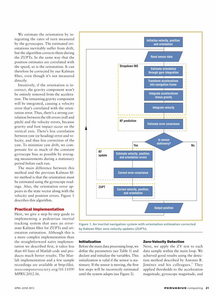
The main difference between this method and the previous Kalman fil-ter method is that the orientation must be estimated using the gyroscope read-ings. Also, the orientation error ap-pears in the state vector along with the velocity and position errors. Figure 1 describes this algorithm.

Practical implementationHere, we give a step-by-step guide to implementing a pedestrian inertial tracking system that uses an error-state Kalman filter for ZUPTs and ori-entation estimation. Although this is a more complex implementation than the straightforward naïve implemen-tation we described first, it takes less than 60 lines of Matlab code and pro-duces much better results. The Mat-lab implementation and a few sample recordings are available at http://doi. ieeecomputersociety.org /10.1109/MPRV.2012.16.

initializationBefore the main data processing loop, we define the parameters (see Table 1) and declare and initialize the variables. This initialization is valid if the sensor is sta-tionary. If the sensor is moving, the first few steps will be incorrectly estimated until the system adapts (see Figure 2).

Zero-Velocity detectionNext, we apply the ZV test to each data sample within the main loop. We achieved good results using the detec-tion method described by Antonio R. Jiménez and his colleagues.7 They applied thresholds to the acceleration magnitude, gyroscope magnitude, and

Figure 1. An inertial navigation system with orientation estimation corrected by Kalman filter zero-velocity updates (ZUPTs).

Initialise velocity, positionand orientation

Read sensor data

Estimate orientationthrough gyro integration

Transform accelerationsinto navigation frame

Integrate accelerationsminus gravity

Integrate velocity

Estimate error covariance

Is sensorstationary? NoYes

KFupdate

KF prediction

Strapdown INS

ZUPT

Estimate velocity, position,and orientation errors

Correct error covariance

Correct velocity, position,and orientation

Output position

PC-12-02-Fis.indd 21 3/21/13 4:27 PM



local acceleration variance. However, a simple threshold on the magnitude of the gyroscope rate-of-turn measure-ments also works well. A ZUPT is ap-plied when w < aw. Isaac Skog and his colleagues confirmed this, showing that their gyroscope-based detector works as well as the one using both ac-celerometers and gyroscopes for typical walking.8

Main loopThe operations in Figure 3 are per-formed for every measurement sample. The sample index, k, is occasionally omitted to simplify notations. For an explanation of the orientation matrix update in steps 4 and 17 in Figure 3, we refer you to work by Honghui Qi and J.B. Moore.9 Dan Simon provides more details regarding the Joseph

form of the covariance update used in step 15.10 The sidebar provides more general references, which cover the gen-eral Kalman filter and inertial naviga-tion equations.

evaluationWe don’t aim to give a precise compari-son of different PDR techniques or to determine optimal parameters. Rather, we want to provide a practical guide, outlining the level of performance you can expect from the standard imple-mentation we’ve described.

Detailed ground truth is difficult to obtain, but even when it’s available, the challenges of aligning it with the esti-mated path and computing position er-rors remain. All position estimates are relative to the initial position and head-ing, and a small error early in the path

can have a significant effect later on, even if no further errors occur.

Researchers have used several meth-ods to evaluate the performance of PDR systems, including

• inspecting estimated paths in the co-ordinate space and comparing them to a simple geometric ground truth;

• computing the distance between starting point and final position esti-mate for a closed loop walk—smaller distances indicate less drift (but this doesn’t account for scaling error);

• computing the estimated total dis-tance travelled, which will give dif-ferent results depending on whether distance is accumulated per measure-ment or per step (and this doesn’t ac-count for heading errors); and

• computing the distance and head-ing error for each step (or segment) by realigning each previous step (or segment) to the ground truth, as Michael Angermann and his col-leagues suggest.11

To evaluate the quality of ZV detec-tion, we compare ZV detection using the IMU to ZV detection using force-sensitive resistors on the sole of the footwear or video recordings of foot movement.

We tested our pedestrian-tracking system with six people. Each subject walked approximately 240 meters in our office building, including sev-eral flights of stairs, in approximately four minutes. We used an XSens MTx sensor (model MTx-28A53G25 or MTx-49A53G25) to record inertial measurements at 120 samples per sec-ond. We use the sensor’s calibrated out-put for precision. These sensors are the standard model with accelerometers with a full scale of ± 50 m/s2 and gy-roscopes with a full scale of ±1,200 °/s. We have since realized that the acceler-ometer range is insufficient for optimal tracking; the ± 180 m/s2 model would have been more suitable. The sensor was attached to the instep of the foot with a Velcro strap.

TABLE 1 System parameter values.

name notation Value

Time step ∆t 1/120 second

Accelerometer noise sa 0.01 m/s2

Gyroscope noise sw 0.01 rad/s (radian per second)

Gravity g 9.8 m/s2

Zero-velocity (ZV) measurement noise su 0.01 m/s

Gyroscope ZV detection threshold sw 0.6 rad/s

Figure 2. Before the main data processing loop, we define the parameters and declare and initialize the variables. Table 1 presents the parameter values.

• Definethezero-velocity(ZV)measurementmatrix:H=(03×303×3I3×3)• DefinetheZVmeasurementnoisecovarianceRasthediagonalmatrixwithvalues vx vy vz

2 2 2σ σ σ

• Initializetheposition:p=(000)T

• Initializethevelocity:v=(000)T

• Initializetheerrorcovariancematrix:P=09×9• InitializetheorientationmatrixCbasedontheaccelerations: roll=arctan a / a( )y

sensorzsensor

pitch= arcsin a /g( )xsensor-

yaw=0 cos pitch sin roll sin pitch cos roll sin pitch

cos roll sin rollsin pitch sin roll cos pitch cos roll cos pitch

=( ) ( ) ( ) ( ) ( )0 ( ) ( )( ) ( ) ( ) ( ) ( )

−−

C

PC-12-02-Fis.indd 22 3/21/13 4:27 PM


Figure 3. Operations performed for every measurement sample. The sample index, k, is occasionally omitted to simplify notations.

1.Computethetimestep∆tfromthepreviousmeasurement.Typically,∆tisconstant.2.Subtractthegyroscopebiasfromthemeasurementsifrequired.3.Computetheskew-symmetricangularratematrixWfromthegyroscopereadings:

00

0k

z y

z x

y x

ΩΩ =

.

-w ww -w-w w

4.Updatetheorientationmatrix:Ck = Ck-1=(2I3×3+Wk∆t)(2I3×3–Wk∆t)-1.9Post-multiplybytheupdatefactor,becausethegyroscopemeasurementsaretakeninthesensorframe.

5.Transformthemeasuredaccelerationsfromthesensorframeintothenavigationframe: = + -( ) 21 /knav

k k ksensora C C a .Usetheaverageofthepreviousandthe

currentorientationestimate,becausemovementhasoccurredbetweenmeasurements(asaroughapproximation).

6.Integratetheaccelerationinthenavigationframeminusgravitytoobtainthevelocityestimate: = - - 2 0 0 g /21 1 tk k knav

knav T( )+ + −

v v a a ∆ .

Usethetrapezemethodofintegration.7.Integratethevelocitytoobtainthepositionestimate:pk=pk-1+(vk+vk–1)∆t/2.8.Constructtheskew-symmetriccross-productoperatormatrixSfromthenavigationframeaccelerations:

=-

--

0

0

0

a a

a aa a

k

znav

ynav

znav

xnav

ynav

xnav

S .

Thismatrixrelatesthevariationinvelocityerrorstothevariationinorientationerrors.9.Constructthestatetransitionmatrix: S

3 3 3 3 3 3

3 3 3 3 3 3

3 3 3 3

tt

k

k

=−

××

× × ×

× ×

× ×

FI 0 00 I I

0 I∆

∆.

10.ConstructtheprocessnoisecovariancematrixQkasthediagonalmatrixwithvalues 0 0 02

tx y z ax ay az( )

∆ .s s s s s sw w w

11.Propagatetheerrorcovariancematrix 1k k k kT

k= +−P F P F Q . Thisisvalidifweassumeprocessnoiseisidenticalonallaxes.12.Detectastationaryphase.

The following operations are only performed for samples occurring in a stationary phase.

13.ComputetheKalmangainKk=PkHT(HPkH

T+R)-1.14.ComputestateerrorsfromtheKalmangainandestimatedvelocity:dk=(dCdPdv)

T=Kkvk.Here,thecompleteerrorvectordiscomposedofthethreeelementsoftheattitudeerror(erroronroll,pitch,andyawangles),thepositionerror,andthevelocityerror,inthatorder.

15.Correcttheerrorcovariance:Pk=(I9× 9-KkH)Pk.Alternatively,usethemorerobustJosephform—seeequation5.19inDanSimon’s Optimal State Estimation.10

16.Constructtheskew-symmetriccorrectionmatrixforsmallangles:

0 [3] [2][3] 0 [1][2] [1] 0

,k

C C

C C

C C

ΩΩεε εε

εε εεεε εε

=−

−−

.e

Theindicesareone-based,sodC [1]isthefirstelementoftheattitudeerror(roll).

17.Correcttheattitudeestimate:Ck=(2I3×3+We,k)(2I3×3-We,k)-1Ck.

9Pre-multiplybythecorrectionfactor,becausethecorrectioniscomputedinthenavigationframe.

18.Correctthepositionestimate:Pk=Pk-dp .19.Correctthevelocityestimate:vk=vk-dv.

PC-12-02-Fis.indd 23 3/21/13 4:27 PM



Figure 4 shows the horizontal and altitude plots from our three imple-mentations: the naive implementa-tion and the Kalman filter implemen-tation (both using the orientations estimated by the built-in AHRS), and the Kalman filter implementa-tion estimating the orientation itself. The fourth pair of plots (Figure 4d) shows the improvement in horizontal position estimates when we manually correct the gyroscope bias. The plots chosen for this article illustrate the improvement achieved for the alti-tude estimates using the Kalman fil-ter for the ZUPTs, and the additional improvement in horizontal position estimates when we compute the ori-entations ourselves and compensate for gyroscope bias.

The difference between subjects and sensors was significant. For some subjects, we couldn’t achieve accurate altitude estimates (there was a drift of up to four meters over the whole walk). On the other hand, some data-sets didn’t require any gyroscope bias correction and produced accurate horizontal plots, even with the simpler implementations. Nevertheless, the Kalman filter implementation with ori-entation estimation and manual gyro-scope bias correction always produced the best results. The stairs are clearly visible at both ends of the building, as well as two detours to avoid seat-ing areas, and even a small kink in the middle of a corridor where the sub-ject paused to open a door. Data re-corded at 120 samples per second gave the best results; lower sample rates displayed degraded performance, but higher rates didn’t bring any noticeable improvement.

We achieved good results with the pedestrian inertial data provided on-line by the team at the German Aero-space Centre.11 We also tested our im-plementation for running. The results were reasonable but would improve considerably if the accelerometers had a wider measurement range to accurately record the foot impacts.

challenges and SuggestionsTwo years ago, we started investigating pedestrian inertial tracking as a com-ponent of a larger multimodal indoor localization system. Since then, we’ve moved from the naïve implementation described earlier to the Kalman filter implementation. More recently, we’ve started estimating the orientation in the algorithm itself. Each new implementa-tion has brought a better understanding of the inner workings of pedestrian in-ertial tracking.

Major causes of Tracking errorsThe gyroscope bias caused most of the horizontal errors observed during our work. We now recalibrate our gyro-scopes before each experiment by re-cording data for 30 to 60 seconds while the sensor isn’t moving. The mean of the gyroscope readings for each axis gives us the bias, which must be subtracted from all measurements before running the PDR algorithm. This method works well even if the sensor is attached to a pedestrian’s foot during calibration. This is a sensor-specific calibration that should be performed again as the components age, or if they’re subject to a violent shock. Although others have included gyroscope and accelerometer bias estimation in their pedestrian in-ertial navigation systems, such meth-ods don’t appear to improve position estimates in the context of pedestrian tracking.

Altitude errors are also common. W. Todd Faulkner and his colleagues have analyzed the altitude errors in in-ertial pedestrian-tracking systems.12 They found that such errors are due to the accelerations of the foot exceed-ing the dynamic range of the acceler-ometers. They noted that accelerations can reach ±10 g when walking, and ±13 g when descending stairs or run-ning. This confirms our own observa-tions and explains why the quality of our altitude estimates varies so much between users with our 5 g accelerom-eters. For the best results, developers should use accelerometers with at least

a ±10 g range and gyroscopes with a ±900 °/s range. Currently, these are rel-atively high specifications for MEMS inertial sensors.

Parameter TuningIt’s reasonable to tune the system pa-rameters to some extent based on sen-sor characteristics and prior knowledge of how the system will be used. How-ever, the system should perform as well as possible for various types of move-ment and without any user-specific training. The choice of one parameter value will affect some of the others. In some cases, a poor choice of one pa-rameter or even an error in the imple-mentation can mask another incorrect parameter. Table 1 lists the parame-ters used in our final implementation. You should get acceptable results with these values, but you might be able to improve the results by further tuning these parameters. John-Olof Nilsson and his colleagues give a more formal analysis of how different parameters affect performance.13 Note that due to an error, the values they give for the noise parameters should be divided by 250 (the sampling frequency).

Step 10 (in Figure 3), which estimates the process noise Q, simply multiplies the gyroscope and accelerometer noise (sw and sa) by the timestep to deter-mine the orientation and velocity noise, and sets position noise to zero. Note that these noise values account for all sources of error in the INS—not only short-term sensor noise but also bias variations, scaling errors, and integra-tion errors. They’re therefore different from the noise values reported in sensor datasheets.

The ZV measurement noise sn, used to construct R, represents the un-certainty in velocity during a ZUPT and should thus be one or two orders of magnitude smaller than an aver-age walking speed of 2 m/s. A more precise ZV detector would require a smaller value, and a less precise one, a larger value. Generally, if the ratio of Q/R remains constant, the system will

PC-12-02-Fis.indd 24 3/21/13 4:27 PM


Figure 4. Plots for a four-minute walk through the Infolab, including stairs at both ends of the building. Each pair of plots shows the horizontal position (left) and altitude (right) for (a) naïve ZUPT, (b) KF ZUPT, (c) KF with orientation estimation, and (d) KF with orientation estimation and gyroscope bias corrections.

0 50 100 150 200 250

–20

–15

–10

–5

0

5

10

Distance travelled (m)

z (m

)

ABCD

Floo

r

–25

15

0 50 100 150 200 250 300–2

0

2

4

6

8

10

12


z (m

)

A

B

C

D

Floo

r0 50 100 150 200 250 300

–2

0

2

4

6

8

10

12


z (m

)

A

B

C

D

Floo

r

–2

0

2

4

6

8

10

12

A

B

C

D

0 50 100 150 200 250 300Distance travelled (m)

z (m

)

Floo

r

(a)

(b)

(c)

(d)

y (m

)

–60 –40 –20 0 20 40

0

10

20

30

40

50

60

70

80

x (m)

StartEnd

y (m

)

–60 –40 –20 0 20 40x (m)

0

10

20

30

40

50

60

70

80 StartEnd

–50 –40 –30 –20 –10 0 10 20

0

10

20

30

40

50

x (m)

StartEnd

y (m

)

–50 –40 –30 –20 –10 0 10 20 30 40

0

10

20

30

40

50

60

x (m)

y (m

)

StartEnd

70

PC-12-02-Fis.indd 25 3/21/13 4:27 PM



perform the same. We recommend set-ting R and then adjusting Q.

We found an approximate value for the gyroscope ZV detection threshold aw by plotting the norm of gyroscope rates of turn over time for a sample pedestrian recording. Periodic stance phases are easy to recognize in such a plot. We set the threshold value slightly higher than the value of the norm dur-ing these phases and then adjusted it to get the best tracking results on the sam-ple recording. This value worked well for all our recordings, but an adaptive threshold could provide a more robust solution.

Output FormatThe output of a PDR system can take several equivalent forms, which should be chosen according to the application. If the system will be used alone, it can simply output the estimated Cartesian coordinates of the pedestrian. If the PDR system is just one component of a larger localization system, it might be more convenient to output incremen-tal values, such as step length, varia-tion in travel direction, and variation

in altitude. Some applications might not require or be able to process posi-tion updates at the high sampling rate of the inertial sensors. In this case, the PDR system should output estimates only once per step, or at a fixed rate.

Tracking the OrientationIn some applications, tracking the yaw of the IMU as well as the direction of travel might be useful. This lets us dis-tinguish between the pedestrian walk-ing forward or backward, which is par-ticularly useful in applications where we want to orient a display accord-ing to the direction the user is facing (rather than the direction in which the user is walking). Assuming the x-axis of the IMU is aligned with the pedes-trian’s forward direction, we can easily compute the yaw from the orientation matrix as yaw – arctan(C2,1/C1,1).

A better way is to use a second IMU attached to the pedestrian’s chest or head and an associated Kalman filter to track the IMU’s position. ZUPTs aren’t possible, but we can assume a constant distance between the two IMUs and in-sert virtual position measurements.

common MistakesDuring our development of PDR sys-tems, we committed several trivial er-rors. Developers shouldn’t confuse the orientation matrix with its transpose; this will give meaningless position es-timates. When updating or correct-ing the orientation matrix, developers must take care to post-multiply or pre-multiply as appropriate. Notations and definitions vary between published works, and we have noted small errors that completely change an equation’s meaning.

We also committed a more funda-mental error by subtracting the accel-eration due to gravity from the mea-sured acceleration immediately after transforming it into the navigation frame. The acceleration due to gravity should indeed be removed during the integration phase. However, it should be left untouched when constructing the skew-symmetric matrix S to pre-serve the correlation between orienta-tion and velocity.

M ore recently, we’ve used this tracking system as the basis for a naviga-tion system for fire-

fighters, which we built using SLAM. So far, we’ve evaluated the navigation system using a video game, but we be-lieve real-world tests will yield promis-ing results.

AcKnOwLEdgmEnTSMany thanks to John-Olof Nilsson at KTH for his invaluable insights into parameter tuning, and to him and others for independently testing our code with their data.

REFEREncES 1. J. Elwell, “Inertial Navigation for the

Urban Warrior,” Proc. of Digitization of the Battlespace IV, SPIE, vol. 3709, 1999, pp. 196–204.

2. E. Foxlin, “Pedestrian Tracking with Shoe-Mounted Inertial Sensors,” IEEE

the AUThORSCarl fischer is a senior research associate in the School of Computing and Communications at Lancaster University, UK. His research interests include pedestrian navigation in uninstrumented environments and robust positioning systems. Fischer received his PhD in computing from Lancaster University. Contact him at [email protected].

Poorna Talkad Sukumar is a project associate in the Computer Science and Automation department at the Indian Institute of Science, Bangalore, India. Her research interests include sensor systems, positioning and navigation, computer vision-based UI, and activity recognition. Talkad Sukumar received her MSc in mobile and ubiquitous computing from Lancaster University. Contact her at [email protected].

Mike Hazas is an academic fellow and lecturer in the School of Comput-ing and Communications at Lancaster University, UK. His research interests include energy and sustainability in everyday life, real world sensing, and algorithms. Hazas received his PhD in computing from the University of Cambridge. Contact him at [email protected].

PC-12-02-Fis.indd 26 3/21/13 4:27 PM


Computer Graphics and Applications, vol. 25, no. 6, 2005, pp. 38–46.

3. S.K. Park and Y.S. Suh, “A Zero Veloc-ity Detection Algorithm Using Inertial Sensors for Pedestrian Navigation Sys-tems,” Sensors, vol. 10, no. 10, 2010, pp. 9163–9178.

4. I. Skog, J.-O. Nilsson, and P. Händel, “Evaluation of Zero-Velocity Detec-tors for Foot-Mounted Inertial Naviga-tion Systems,” Proc. 2010 Int’l Conf. Indoor Positioning and Indoor Navi-gation, extended abstract, IEEE, 2010, pp. 172–173.

5. J. Callmer, D. Törnqvist, and F. Gustafs-son, “Probabilistic Stand Still Detection Using Foot Mounted IMU,” Proc. 13th Int’l Conf. Information Fusion, IEEE, 2010, pp. 1–7.

6. Ö. Bebek et a l . , “Personal Navi-gat ion v ia High-Resolut ion Gait-Corrected Inertial Measurement Units,”

IEEE Trans. Instrumentation and Measurement, vol. 59, no. 11, 2010, pp. 3018–3027.

7. A. Jiménez et al., “Indoor Pedestrian Navigation Using an INS/EKF Frame-work for Yaw Drift Reduction and a Foot-Mounted IMU,” Proc. of Work-shop on Positioning, Navigation and Communication (WPNC 10), IEEE, 2001, pp. 135–143.

8. I. Skog et al., “Zero Velocity Detection—An Algorithm Evaluation,” IEEE Trans. Biomedical Eng., vol. 57, no. 11, 2010, pp. 2657–2666.

9. H. Qi and J. B. Moore, “Direct Kalman Filtering Approach for GPS/INS Inte-gration,” IEEE Trans. Aerospace and Electronic Systems, vol. 38, no. 2, 2002, pp. 687–693.

10. D. Simon, Optimal State Estimation: Kalman, H Infinity, and Nonlinear Approaches, John Wiley, 2006.

11. M. Angermann et al., “A High Pre-cision Reference Data Set for Pedes-trian Navigation Using Foot-Mounted Inertial Sensors,” Proc. 2010 Int ’l Conf. Indoor Positioning and Indoor Navigation (IPIN 10), IEEE, 2010, pp. 1–6.

12. W.T. Faulkner et al., “Altitude Accu-racy While Tracking Pedestrians Using a Boot-Mounted IMU,” Position Location and Navigation Symposium (PLANS 10), IEEE, 2010, pp. 90–96.

13. J.-O. Nilsson, I. Skog, and P. Händel, “Performance Characterisation of Foot-Mounted ZUPT-Aided INSs and Other Related Systems,” Proc. 2010 Int’l Conf. Indoor Positioning and Indoor Naviga-tion, extended abstract, IEEE, 2010, pp. 182–183.

Selected CS articles and columns are also available for free at http://ComputingNow.computer.org.

IEEE Computer Society’s Conference Publishing Services (CPS) is now offering conference program mobile apps! Let your attendees have their conference schedule, conference information, and paper listings in the palm of their hands.

The conference program mobile app works for Android devices, iPhone, iPad, and the Kindle Fire.

CONFERENCESin the Palm of Your Hand

For more information please contact [email protected]

PC-12-02-Fis.indd 27 3/21/13 4:27 PM

implementing a pedestrian tracker using inertial …hazas/fischer13_implementinga...implementing a...

Documents