implementation of genetic algorithms in fpga-based
TRANSCRIPT

Clemson UniversityTigerPrints
All Theses Theses
8-2009
Implementation of Genetic Algorithms in FPGA-based Reconfigurable Computing SystemsNahid AlamClemson University, [email protected]
Follow this and additional works at: https://tigerprints.clemson.edu/all_theses
Part of the Electrical and Computer Engineering Commons
This Thesis is brought to you for free and open access by the Theses at TigerPrints. It has been accepted for inclusion in All Theses by an authorizedadministrator of TigerPrints. For more information, please contact [email protected].
Recommended CitationAlam, Nahid, "Implementation of Genetic Algorithms in FPGA-based Reconfigurable Computing Systems" (2009). All Theses. 618.https://tigerprints.clemson.edu/all_theses/618

IMPLEMENTATION OF GENETIC ALGORITHMS IN FPGA-BASED RECONFIGURABLE COMPUTING SYSTEMS
A Thesis Presented to
the Graduate School of Clemson University
In Partial Fulfillment of the Requirements for the Degree
Master of Science Computer Engineering
by Nahid Mahfuza Alam
August 2009
Accepted by: Dr. Melissa C. Smith, Committee Chair
Dr. Walter B. Ligon III Dr. Mary E. Kurz

ii
ABSTRACT
Genetic Algorithms (GAs) are used to solve many optimization problems in
science and engineering. GA is a heuristics approach which relies largely on random
numbers to determine the approximate solution of an optimization problem. We use the
Mersenne Twister Algorithm (MTA) to generate a non-overlapping sequence of random
numbers with a period of 219937-1. The random numbers are generated from a state vector
that consists of 624 elements. Our work on state vector generation and the GA
implementation targets the solution of a flow-line scheduling problem where the flow-
lines have jobs to process and the goal is to find a suitable completion time for all jobs
using a GA. The state vector generation algorithm (MTA) performs poorly in traditional
von Neumann architectures due to its poor temporal and spatial locality. Therefore its
performance is limited by the speed at which we can access memory. With an
approximate increase of processor performance by 60% per year and a drop of memory
latency only 7% per year, a new approach is needed for performance improvement. On
the other hand, the GA implementation in a general-purpose microprocessor, though
performs reasonably well, has scope for performance gain in a parallel implementation.
The parallel implementation of the GA can work as a kernel for applications that uses a
GA to reach a solution. Our approach is to implement the state vector generation process
and the GA in an FPGA-based Reconfigurable Computing (RC) system with the goal of
improving the overall performance.
Application design for FPGA-based RC systems is not trivial and the performance
improvement is not guaranteed. Designing for RC systems requires algorithmic

iii
parallelism in order to exploit the inherent parallelism of the FPGA. We are using a high-
level language that provides a level of abstraction from the lower-level hardware in the
RC system making it difficult to fully exploit some of the architectural benefits of the
FPGA. Considering these factors, we improve the state vector generation process
algorithmically. Our implementation generates state vectors 5X faster than the previous
implementation in an Intel Xeon microprocessor of 2GHz. The modified algorithm is also
implemented in a Xilinx Virtex-4 FPGA that results in a 2.4X speedup. Improvement in
this preprocessing step accelerates GA application performance as random numbers are
generated from these state vectors for the genetic operators. We simulate the basic
operations of a GA in an FPGA to study its behavior in a parallel environment and
analyze the results. The initial FPGA implementation of the GA runs about 7X slower
than its microprocessor counterpart. The reasons are explained along with suggestions for
improvement and future work.

iv
DEDICATION
I dedicate this work to all of them who continually encourage me strive for the best.
v
ACKNOWLEDGMENTS
First I would like to express my gratefulness to the Almighty for providing me the
light and enabling me to finish this work.
My deepest gratitude goes to my advisor, Dr. Melissa Smith for her guidance and
support that made this work possible. Her approach towards solving a problem and
continual support for growth has shown me the path to excel. I would like to thank Dr.
Mary Kurz for her warmth approach that introduced me in the field of Operational
Research. I would also like to thank my committee members for their review and
valuable comments on this thesis.
I thank my parents, younger brother and other family members for always being
with me and supporting me in time of my need.
My sincere gratitude goes to the members of Future Computing Technology lab
of Clemson University for their support and cooperation. I would like to thank Andrew
Woods of University of Cape Town for all his cooperation in understanding Nallatech
tools and hardware. My thanks to Ayub of Bangladesh University of Engineering and
Technology for his prompt solution with problems I had in UNIX. Thanks to Yujie Dong
of Clemson University for his help with LATEX template. I express my appreciation to
Nallatech support for their cooperation in technical details and prompt responses that
helped in accelerating the work.
Finally, I would like to thank Clemson University for the financial support and
excellent academic environment throughout the program.

vi
TABLE OF CONTENTS
Page
TITLE PAGE .................................................................................................................... i ABSTRACT ..................................................................................................................... ii DEDICATION ................................................................................................................ iv ACKNOWLEDGMENTS ............................................................................................... v LIST OF TABLES ........................................................................................................ viii LIST OF FIGURES ........................................................................................................ ix CHAPTER 1. INTRODUCTION ......................................................................................... 1 2. BACKGROUND ........................................................................................... 7 2.1 Genetic Algorithms and Flow-Line Scheduling ...................................... 7 2.1.1 Anatomy of a Genetic Algorithm ................................................... 7 2.1.2 Modeling Optimization Problems into Genetic Algorithms ............................................................................ 9 2.1.3 Mersenne Twister Algorithm ........................................................ 14 2.2 Related Research .................................................................................... 17 2.3 Our Approach......................................................................................... 18 3. DESIGN AND IMPLEMENTATION ........................................................ 19 3.1 Hardware/Software Partitioning ............................................................ 19 3.1.1 MTA Partitioning Analysis ........................................................... 21 3.1.2 GA Partitioning Analysis .............................................................. 22 3.2 Systems and Tools Used ........................................................................ 28 3.3 Implementation Models ......................................................................... 30 3.4 Accelerating State Vector Generation ................................................... 32 3.5 Implementing Genetic Algorithms in FPGAs........................................ 37 3.6 Limitations of the Design....................................................................... 39 3.7 Summary ................................................................................................ 42

vii
Table of Contents (Continued) Page 4. PERFORMANCE AND RESULT ANALYSIS ......................................... 43 4.1 Performance Improvement of State Vector Generation ................... 43 4.2 GA Performance Analysis ............................................................... 49 5. CONCLUSION AND FUTURE WORK .................................................... 56
5.1 Conclusion ....................................................................................... 56 5.2 Future Work ..................................................................................... 58 REFERENCES .............................................................................................................. 63

viii
LIST OF TABLES
Table Page 4.1 Performance Data of State Vector Generation Using MTA Algorithm ........................................................................................... 44 4.2 Resource Utilization of State Vector Generation Algorithm ....................... 47 4.3 Performance Data of Basic GA Operations ................................................. 49 4.4 Resource Utilization of GA Operations ....................................................... 53
ix
LIST OF FIGURES
Figure Page 2.1 Anatomy of a Genetic Algorithm .................................................................. 8 2.2 The Crossover Operation in a GA ................................................................ .9 2.3 The Mutation Operation in a GA ................................................................... 9 2.4 The Flow-Line Scheduling Problem ............................................................ 10 2.5 Mapping Problem Data to Solution Space ................................................... 12 2.6 Saving State Vectors of MTA ...................................................................... 16 2.7 Mersenne Twister Algorithm – MT19937 ................................................... 16 3.1 Flat Profile of GA Process ........................................................................... 23 3.2 Snap Shot of the Overall Call Graph ........................................................... 24 3.3 Call Graph for 1st Partition Evaluation ........................................................ 25 3.4 Call Graph for 2nd Partition Evaluation ....................................................... 25 3.5 Functional Diagram of H101 PCI-XM ........................................................ 29 3.6 Location of the FPGA in the Memory Hierarchy ........................................ 31 3.7 Original MTA Algorithm ............................................................................. 34 3.8 Improved MTA for State Vector Generation ............................................... 35 3.9 MTA Implementation in an FPGA .............................................................. 36 3.10 Design of Basic GA Functions in the FPGA ............................................... 38 3.11 Flow-Chart of the Overall GA Implementation ........................................... 39

x
List of Figures (Continued) Figure Page 3.12 Random Number Generation in Parallel Using a FIFO ............................... 41 4.1 Initchrom Function in General-Purpose Microprocessor ............................ 50 4.2 ParaUnifCross Function in General-Purpose Microprocessor .................... 52
CHAPTER 1
INTRODUCTION
Genetic Algorithms have important applications in problems related to
optimization, machine learning, game theory, design automation, evolvable hardware,
distributed systems, network security, bioinformatics and many more. Genetic
algorithms are iterative procedures that work on groups of solution representations called
chromosomes. Each chromosome is composed of smaller segments of data called genes.
A set of chromosomes together form a population. We generally initialize each gene in
each chromosome randomly. The basic iterative work of the genetic algorithm is
evolution from one population say t, to the next population, t+1. This evolution is done
through the application of genetic operators – Selection, Crossover and Mutation, which
introduce many random elements from one population to the next. Through this iterative
procedure, the solution of the optimization problem evolves toward a better one.
This research is based on the work of Kurz [1] on scheduling industrial flow-lines.
These flow-lines have sequence-dependent setup time, i.e. setup times depend on the
order jobs are scheduled to the machines. The flow-line has several stages in series. Each
stage contains a different number of machines and each machine has different jobs.
Machines in parallel are identical in capability and processing rate. The flow-line is
flexible in the sense that jobs may skip stages. Given the above conditions, the problem
is to find a schedule that will result in an acceptable completion time of all jobs. The
sequence dependent setup time makes this a general case of the Travelling Salesman
Problem (TSP), and thereby an NP-Hard optimization problem. The solution
2
representation of this flow-line scheduling problem is analogous to the chromosomes in
the GA representation.
For the purpose of this research, chromosomes of a GA represent the order in
which jobs are processed in one stage. There are other versions of the algorithm where
chromosomes represent jobs in more than one stage. But for this algorithm, the order of
jobs in the remaining stages depends on the order of jobs at the first stage only. That is,
randomness comes into play only at the first stage and all other stages are deterministic.
Each gene of a chromosome has a value that is generated randomly. Based on these
values, jobs are sorted and assigned to machines. The goal is to find a combination of
jobs in stages that will result in a satisfactory makespan for the flow-line, where
makespan is the max completion time of all jobs. Through various genetic operations like
Crossover and Mutation, the GA tries to reach this goal. These genetic operations
introduce randomness in the GA process.
After each iteration of the GA, a specific set of genetic operators and parameters
known as a configuration is obtained. To arrive at a better solution for the optimization
problem, we must determine which configuration is better. That is, which configuration
results in the lowest makespan for the flow-line scheduling. To obtain different
configurations, we need an independent set of random numbers. If one iteration of a GA
uses upto 600 million random numbers, 600 million random numbers are needed to
produce one configuration. In order to facilitate appropriate statistical analysis, the sets of
random numbers should be non-overlapping, so that the assumption of independent sets
of random numbers can be made. The Mersenne Twister Algorithm [2] facilitates this, as

3
it has a period of 219937-1, meaning it can provide sufficient random numbers before
repeating. This period is in contrast to the basic rand function in the standard C library,
which has a period of just over 32,600.
For solving the flow-line scheduling problem, researchers generally consider three
different versions of the GA. We call each of them an algorithm. In order to determine
reasonable performance measures, most GA research requires each algorithm to be
executed many times [3,4], such as 50 times, per input data set. The input data set for the
flow-line scheduling problem consists of number of stages, number of machines per
stage, number of jobs and setup, and ready and processing time for each job. The flow-
line scheduling may have different problem types, i.e. scheduling may be for different
industries leading to different requirements. The input values of the data set may vary,
resulting in different input files. For our optimization problem, there are 180 different
problem types, 10 different input files for each with 3 different algorithms, totaling 5,400
files. If we consider only the simplest algorithm, then one replication (180x10=1,800 files
per algorithm) requires 45 hours in a single core Pentium IV 3GHz HT machine which
would scale to 80 days of run time to complete the necessary 50 replications of a single
data set. Kurz abandoned this research approach due to the immense computational time
until discovering the task parallelism potential of Condor Grid computing.
However, while the introduction of the grid environment of Condor removed the
barriers of excessive computational time, managing the random number usage became
problematic. Though the use of MTA solves the problem of generating a non-
overlapping sequence of random numbers, ensuring that each run uses a non-overlapping

4
stream of random numbers generated from the same seed for replicability must be
considered. For example, we could use the first set of 600 million numbers for iteration
1, then the second set for iteration 2. In a traditional computing environment, we could
just allow the 2nd iteration to start when the 1st iteration left off. But in grid computing,
iteration 1 and 2 may be running simultaneously. In that case, iteration 2 must first
generate and throw away 600 million random numbers and then begin its work. This
approach, while functionally correct, requires over 4,000 days to burn through the 600
million numbers before reaching the second set on the 250,000th iteration. Each iteration
requires approximately 45 hours of computation time making the overhead unacceptable.
In contrast, we could generate the random numbers offline and store them as an
additional input file for each run. However, storage becomes an issue as the file size for
600 million numbers requires over 3 GB. The 50 replications required for just one data
set equates to 150 GB of storage. Again, while the idea is nominally feasible for a small
experiment, the storage requirements render this approach infeasible for the general case.
Fortunately, the MTA has an internal state, which is exposed in a structure
composed of one integer and 624 values of unsigned integer or unsigned long. So, while
we echo the sentiment of generating many random numbers offline, we only need to store
the algorithm state, in a state file, at set intervals. Then, we can read in the state
information and begin the new generation from that point, reducing the storage space
requirement. In previous work, Kurz has generated and saved 360,000 state files that are
1 billion random numbers apart. This generation took about 22 days to complete on a
dual core AMD Opteron 885 @ 2.6 GHz.

5
Due to their inherent parallelism, FPGAs are well suited for applications that have
some form of parallelism in their characteristics. If an application can be designed in a
way so that it can exploit the parallelism of an FPGA, we can have a significant
performance gain over its general-purpose microprocessor counterpart. As FPGAs run at
a much lower clock frequency, any performance gain is achieved at much lower power.
But these gains are not free of cost. The price is paid in terms of resource utilization.
FPGAs are equipped with on chip resources like Block RAM, DSP units and on-board
memories like SRAM, SDRAM etc. An application must maximize the utilization of
these resources to maximally exploit the inherent parallelism of an FPGA.
In this thesis, we present an improved state file generation algorithm which is 5X
faster than its previous implementation on an Intel Xeon 5130@2GHz. Porting this code
to an FPGA gives a modest 2.4X speedup due to several conditional statements that limit
the performance. For our purpose, we must save state vectors at one billion number
intervals, meaning we need to iterate through the original MTA algorithm one billion
times before saving one state vector. We modify the algorithm such that it does not need
to iterate one billion times. Also we eliminate the random number tempering portion of
the original MTA algorithm as those are not required when generating state files. These
two factors provide the speedup while generating state vectors. The previous GA
implementation of this flow-line scheduling problem was designed for a traditional von
Neumann architecture. After profiling the original code, hardware suitable functions were
implemented on the FPGA. We implement the basic computations of the GA in an FPGA
and study its performance while generating and feeding the random numbers to the GA

6
process inside the FPGA. The performance is compared to its original implementation in
a general-purpose microprocessor. A comprehensive analysis of result is given along with
directions for future improvements.
We summarize the results as follows:
• Speedup in state vector generation using the Mersenne Twister Algorithm:
5X in general-purpose microprocessor and 2.4X in an FPGA.
• A comprehensive study of the simulation results and measured data of basic
GA operations implemented in an FPGA.
The remainder of this thesis is organized as follows. Chapter II provides background
information, which includes a general description of Genetic Algorithms, how it is used
to solve the optimization problem of flow-line scheduling, justification for using MTA,
and the systems and tools used to conduct the experiments. Chapter III discusses how
different components of these experiments were modeled to fit within the constraints of
the FPGA–based systems used and also discusses the limitations of our design. Chapter
IV analyzes the performance and results of the random number generation and Genetic
Algorithm simulation process. And finally Chapter V offers conclusions and directions
for potential solutions of the limitations of our design.
7
CHAPTER 2
BACKGROUND
This chapter discusses how the solution of the flow-line scheduling problem is
analogous to Genetic Algorithms, some previous work on MTA and GA implementations
on FPGAs, and how our solution differs from them.
2.1 Genetic Algorithms and Flow Line Scheduling
In this research, the solution of a flow line scheduling problem is represented in
terms of chromosomes and genes of a Genetic Algorithm. In this section, we will discuss
GA details, how a flow-line scheduling is mapped to a GA, and why the Mersenne
Twister Algorithm is used in this research.
2.1.1 Anatomy of a Genetic Algorithm
Genetic Algorithm, a heuristic based approach for solving optimization problems,
was introduced by Holland [9]. A typical GA has two steps [5]: a representation of the
solution domain that reflects the genetic representation in a genome and a fitness function
to evaluate the fitness of the current representation. The solution representations are
generally in bits but may vary based on the application. For example, for our flow-line
scheduling problem, we have a double-precision floating-point representation. GAs
employ the following general steps: Initialization, Selection, Crossover, and Mutation.
The algorithm starts with the random initialization of the initial population. Each
population has a number of chromosomes and each chromosome has a number of genes.
Each gene is also initialized by a random number. In this research, we generate the
random numbers using the Mersenne Twister Algorithm [2], which is further explained in
8
section 2.1.3. After initialization, two parents are selected to generate their successor
during the Selection stage. This selection is based on a fitness function [5] as parents of
higher fitness values are expected to produce a better next generation. To generate the
successor, the GA uses the Crossover operation where a crossover point is selected
randomly. In the successor, solutions from the first parent are selected before the
crossover point. Solutions after the crossover point are taken from the second parent. After
Crossover, the Mutation operation is applied to increase the probability of the fitness of
the solution. In Mutation, a random gene of the successor chromosome is changed with
some probability. This process continues until the stopping criteria are satisfied. The
probability of Mutation is a constant that is dependent on the application. Theoretically,
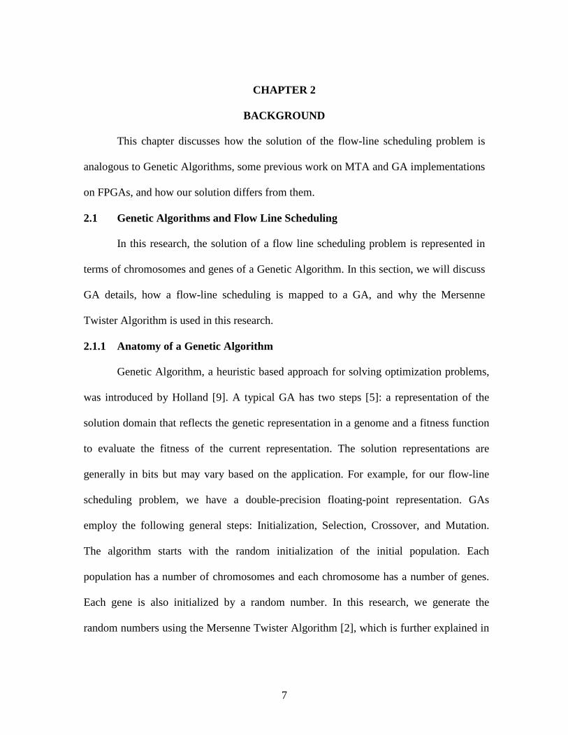
the best set of chromosomes is expected to survive eventually. The overall GA process is
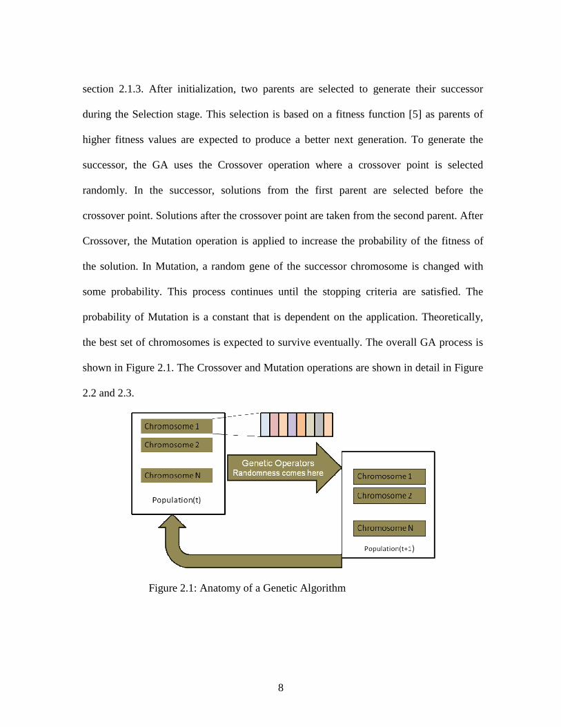
shown in Figure 2.1. The Crossover and Mutation operations are shown in detail in Figure
2.2 and 2.3.
Figure 2.1: Anatomy of a Genetic Algorithm
9
Figure 2.2: The Crossover Operation in a GA
Figure 2.3: The Mutation Operation in a GA
In this research, the Mutation operation of the GA is replaced by the Immigration
operation. In Mutation, one specific gene of a chromosome is changed with some
probability. But in Immigration, a fresh new set of chromosomes are immigrated into the
next generation of the population. That is, all genes of those chromosomes are replaced
with a random value. How many chromosomes will be immigrated depends on a
predefined constant and is generally determined by the given optimization problem.
2.1.2 Modeling Optimization Problems into Genetic Algorithms
Our target optimization problem is a flow-line scheduling problem that is very
common in industrial manufacturing. These manufacturing systems have taken many
forms with the added complexity of limited resources, time constraints, complicated
process plans etc. For example, flow-lines of the semiconductor industry have multiple
10
machines in each stage and jobs revisit previous stages multiple times [1]. Another
example is in the printed circuit board industry where jobs may skip stages depending on
the circuit board specification. Each of these industries has different scheduling
objectives but minimizing the overall completion time of all jobs, i.e. makespan can be
considered a generic goal. These common goals are why operation researchers have
focused on the makespan criterion for optimization.
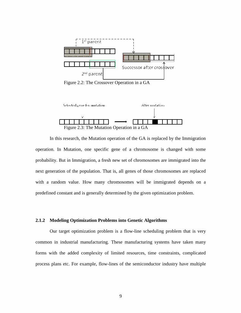
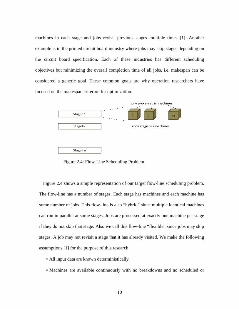
Figure 2.4: Flow-Line Scheduling Problem.
Figure 2.4 shows a simple representation of our target flow-line scheduling problem.
The flow-line has a number of stages. Each stage has machines and each machine has
some number of jobs. This flow-line is also “hybrid” since multiple identical machines
can run in parallel at some stages. Jobs are processed at exactly one machine per stage
if they do not skip that stage. Also we call this flow-line “flexible” since jobs may skip
stages. A job may not revisit a stage that it has already visited. We make the following
assumptions [1] for the purpose of this research:
• All input data are known deterministically.
• Machines are available continuously with no breakdowns and no scheduled or
11
unscheduled maintenance.
• Jobs are non-preemptive, processed without error, and have no associated priority.
• Jobs are available for processing at a stage as soon as they have finished
processing at the previous stage.
• The ready time for a job is the maximum time it takes to complete processing in
the previous stages.
• Non-anticipatory sequence dependent setup times exist between jobs at a stage.
• Machines cannot be blocked because the current job has nowhere to go, i.e.
infinite buffer exists before, after, and between stages.
• Machines in parallel are identical in capabilities and processing rate.
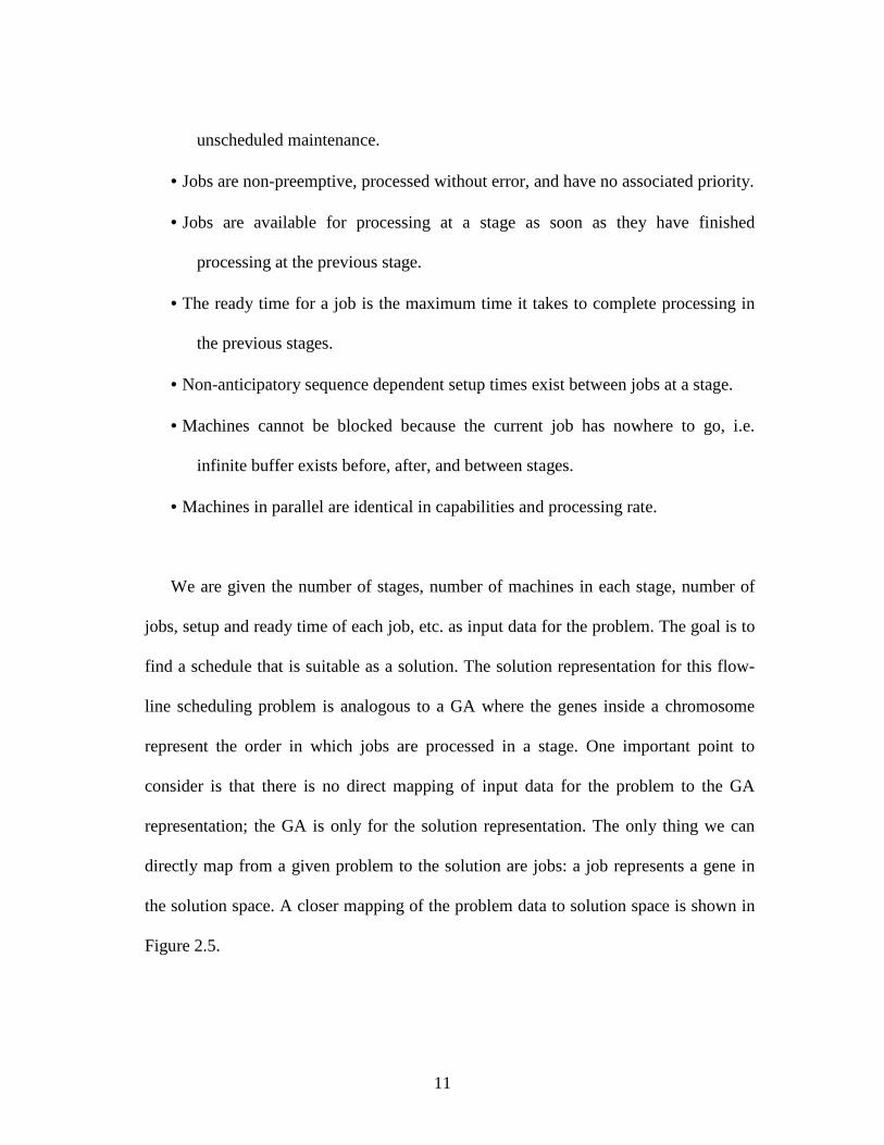
We are given the number of stages, number of machines in each stage, number of
jobs, setup and ready time of each job, etc. as input data for the problem. The goal is to
find a schedule that is suitable as a solution. The solution representation for this flow-
line scheduling problem is analogous to a GA where the genes inside a chromosome
represent the order in which jobs are processed in a stage. One important point to
consider is that there is no direct mapping of input data for the problem to the GA
representation; the GA is only for the solution representation. The only thing we can
directly map from a given problem to the solution are jobs: a job represents a gene in
the solution space. A closer mapping of the problem data to solution space is shown in
Figure 2.5.

12
Fig 2.5: Mapping Problem Data to Solution Space.
To express the problem and the stopping criteria addressed in this research, we
use the following definitions [1]:
n number of jobs to be scheduled
g number of serial stages
mt number of machines at stage t
pti processing time for job i at stage t (assumed to be integral)
stij setup time from job i to job j at stage t
St set of jobs that visit stage t = { i : pti >0}
z makespan
For this flow-line scheduling problem, we apply the restriction that each stage
must be visited by at least as many jobs as there are machines in that stage. If this is not

13
true then there is no problem for job scheduling. The goal is to find a feasible solution
subject to many constraints. We can formulate the problem [1] as:
P: min z (1)
That is, we want to minimize makespan. So eq. (1) is our objective function.
For this flow-line scheduling problem, we also make the following assumptions [1]:
• Stages are independent except that stage t’s completion time is stage t+1’s
ready time.
• Setup times are such that an optimal solution will always exist.
Each chromosome is evaluated to check whether it satisfies some stopping criteria,
i.e. whether the current schedule results in an optimal solution. The optimal solution for a
specific problem needs to meet the lower bound requirement defined by eq. (2) and (3).
(2)
(3)
LB(1) is a job based bound and LB(2) is machine based [1]. For the job based bound,
every job must be setup and processed at every stage. Setup requires minimal amount of
time for setting up job i. For the machine based bound, every stage t needs time for
processing job 0. It also needs time for preemptive processing and a minimal setup time
for the rest of the jobs. We can also consider minimal time to get to the stage and
minimal time after finishing that stage. In our implementation, we consider the larger of

14
these two lower bounds as our stopping criteria. Once the best chromosome’s makespan
hits that lower bound, we stop our iterations of the GA. Otherwise we continue evaluating
all the chromosomes with basic GA operations until we exhaust all of them or hit a lower
bound, whichever comes first.
2.1.3 Mersenne Twister Algorithm
As evident from the GA process, its operation largely depends on random
numbers. For this implementation, the random numbers are generated using the
Mersenne Twister Algorithm [2]. MTA is a uniform pseudo random number generator.
It has a period of 219937-1 and 623-dimensional equidistribution up to 32 bit accuracy
[2]. Such a long period implies that it generates 219937-1 random numbers before
repeating. This non-overlapping sequence is large enough for our problems of intent.
Also the very high order of dimensional equidistribution implies that there is very
negligible correlation between successive values of output sequence [10]. MTA passes
diehard tests [22] and numerous other tests of randomness [23]. This algorithm is
designed specifically for Monte Carlo and other statistical simulations, but it is not
suitable for Cryptography as observing a sufficient number of iterations (624 in this
case) will lead one to predict the rest of the iterations. In this research, MTA is chosen
because of its long non-overlapping period.
MTA is a twisted feedback generalized shift register [11], the algorithm is based
on the recurrence relation eq. (4):
(4)
Axxxx lk
ukmknk )|(: 1+++ ⊕=

15
Here,
n degree of recurrence
w word width (in number of bits)
m middle word or the number of parallel sequences, nm ≤≤1
u,l Mersenne Twister tempering bit shift
x a word of width w
xl,xu x with lower and upper mask applied
A matrix that contains twist information
k constant with values 0,1,…
Figure 2.7 shows the MTA algorithm that generates 32-bit random numbers. As
mentioned earlier, we require a maximum of 600 million random numbers.
One interesting advantage of MTA is that random numbers can be generated from
a state vector that was saved before actually generating the numbers. These state vectors
work as an entry point for a specific sequence of random numbers. State vectors are the
specific states of the MTA after a sequence of random numbers and can be later used to
regenerate the same sequence of random numbers. Though for this project, we need a
maximum of 600 million random numbers, vectors are saved after one billion for more
general-purpose use. Although saving state vectors at one billion number intervals adds
to the poor performance of state vector generation process, this has the benefit of lower
storage requirement (fewer state vectors). Figure 2.6 shows a snap shot of this process.
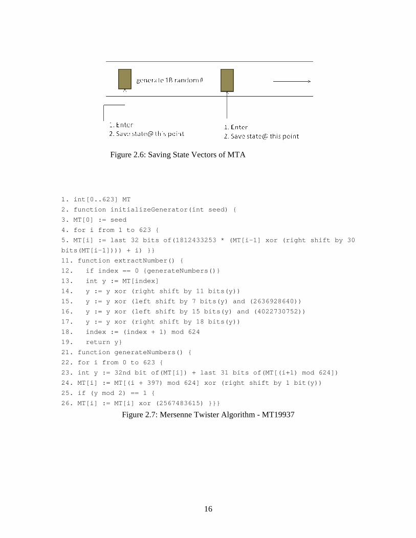
16
Figure 2.6: Saving State Vectors of MTA
1. int[0..623] MT
2. function initializeGenerator(int seed) {
3. MT[0] := seed
4. for i from 1 to 623 {
5. MT[i] := last 32 bits of(1812433253 * (MT[i-1] xor (right shift by 30
bits(MT[i-1]))) + i) }}
11. function extractNumber() {
12. if index == 0 {generateNumbers()}
13. int y := MT[index]
14. y := y xor (right shift by 11 bits(y))
15. y := y xor (left shift by 7 bits(y) and (2636928640))
16. y := y xor (left shift by 15 bits(y) and (4022730752))
17. y := y xor (right shift by 18 bits(y))
18. index := (index + 1) mod 624
19. return y}
21. function generateNumbers() {
22. for i from 0 to 623 {
23. int y := 32nd bit of(MT[i]) + last 31 bits of(MT[(i+1) mod 624])
24. MT[i] := MT[(i + 397) mod 624] xor (right shift by 1 bit(y))
25. if (y mod 2) == 1 {
26. MT[i] := MT[i] xor (2567483615) }}}
Figure 2.7: Mersenne Twister Algorithm - MT19937
17
2.2 Related Research
There are a number of publications that discuss implementing the Mersenne
Twister Algorithm and Genetic Algorithms in FPGAs. Ishaan et al. [6] did parallel
implementations of 32, 64, 128–bit SIMD MTA on Xilinx Virtex–II Pro FPGAs. They
used interleaved and chunked parallelism and showed how the ‘jump ahead’ technique
can produce multiple independent sequences to yield higher throughput. Shrutisagar et al.
[12] worked on partial pipelining and sub-expression elimination to increase the
throughput per clock cycle on the RC1000 FPGA Development platform that is equipped
with Xilinx XCV2000E FPGAs. Both FPGA implementations of MTA used VHDL
whereas ours is implemented in High-Level Language DIME-C [18]. Hossam et al. [7]
implemented the basic GA modules along with the random number generator module in
three different types of Xilinx FPGAs: XC4005, SPARTAN2 XC2S100-5-tq144, and
Virtex XCV800 using VHDL and Mentor Graphics tools. They tested their design in
applications ranging from thermistor data processing, linear function interpolation, and
computation of vehicle lateral interpolation to test how the design performs with respect
to producing the optimal solutions. Tatsuhiro et al. [8] designed two tools to facilitate the
hardware design of GAs to predict the synthesis results based on input parameters,
number of parallel pipelines, etc. Edson et al. [13] implemented a parallel and
reconfigurable architecture for synthesizing combinational circuits using GAs. Paul and
Brent [14] implemented a parallel GA for optimizing symmetric Traveling Salesman
Problem (TSPs) using Splash 2. Emam et al. [15] introduced an FPGA- based GA for
blind signal separation.

18
2.3 Our Approach
In all the previous research, the MTA or GA is a customized implementation
specifically targeting the architecture, in this case FPGAs. Our approach significantly
differs as we try to accelerate an existing application originally designed for von
Neumann architectures. Both approaches have their own advantages and disadvantages.
In the previous research, though they have achieved a performance gain in GA process,
they do not consider how it performs when the GA works as a part of a larger application.
In our approach, the probability of overall application acceleration is low as the original
application design never considered exploiting parallelism. But this approach
demonstrates what can happen when the GA is a small part of an application which was
not originally designed for a parallel architecture. Also it shows us the necessity of
designing and implementing an application specifically to take advantage of the parallel
architecture. Our approach uses the high-level language DIME-C, but to the best of our
knowledge, all the previous work used hardware description languages such as VHDL or
Verilog.

19
CHAPTER 3
DESIGN AND IMPLEMENTATION
Our design and implementations are divided into two main parts. The first step is
to design and implement state vector generation process in the FPGA. These state vectors
are an integral part of the GA as they are used to generate the required random numbers.
The second step is to design and implement the basic GA operations in an FPGA along
with the generation of random numbers from the previously stored state vectors. Before
designing the system for FPGA implementation, we conducted function profiling of the
existing GA implementation that was written for a general-purpose microprocessor. From
the profile data, we identified critical code segments for possible implementation in the
FPGA and analyzed the issues related to hardware/software partitioning. We designed an
improved algorithm for generating state vectors using the MTA which is 5X faster than
its previous implementation in a general-purpose microprocessor and 2.4X faster than the
previous FPGA implementation. We also implemented the basic GA operations in an
FPGA. This chapter discusses and justifies our hardware/software partitioning approach,
systems and tools used, implementation model, and design and implementation
techniques for the state vector generation and GA operations. Finally we discuss the
limitations of our approach.
3.1 Hardware/Software Partitioning
For a given application, a hardware/software partition maps each region of the
application onto hardware (ASIC or Reconfigurable Logic) or software (microprocessor).

20
That is, a partition is a complete mapping of an application to either hardware or
software. The goal of the partition is to maximize performance within the constraint of
limited resources, in this case one Xilinx Virtex-4 LX100 FPGA.
There are several issues to consider for hardware/software partitioning. Some of them
are listed below:
• Granularity: types of regions to consider.
• Partition evaluation: determining the goodness of the partition.
• Alternative region implementation: alternatives of hardware implementation.
• Implementation model: interfacing between microprocessor and FPGA.
• Exploration: finding good solution quickly.
Granularity is of two types: coarse and fine. If we partition based on tasks, functions
and loops, that is called coarse-grained partitioning. On the other hand, fine-grained
partitioning partitions regions based on code blocks, statements and operations. Both
approaches have their own advantages and disadvantages. Therefore a heterogeneous
granularity may be considered to take advantage of both extremes. The most intuitive
approach to partitioning an application is based on its functions, i.e. coarse-grained
partitioning. Also, coarse-grained partitioning may result in more accurate estimations
during partition evaluation as it does not require the combination of several small regions
and their communication overhead. An important disadvantage of coarse-grained
partitioning is that it often has less inter-partition communication. That means, more data
communication occurs between the host processor and FPGA than among different

21
Processing Elements (PEs) inside the FPGA. This situation may outweigh the benefit of
implementing regions in hardware as the hardware/software communication is generally
expensive. On the other hand, fine-grained partitioning gives more control over the
exploitation of parallelism and less communication overhead between host processor and
FPGA. But it is not intuitive and so generally takes longer to find a good partition. Also,
estimation during partition evaluation is more difficult in this case due to their inter-
partition communication.
We use gprof for function profiling of the original GA implementation that was
targeted for a general-purpose microprocessor. After profiling, we have two types of
profile data: flat profile and call graph.
3.1.1 MTA Partitioning Analysis
The hardware/software partitioning for state vector generation using MTA is
straightforward. We did not profile the MTA implementation as the main computation
occurs in a single function called genrand_32. Therefore it is obvious that we have to
implement that function in the FPGA. The partitioning of the MTA is a coarse-grained
partitioning. We did not explore any other alternative regions for the FPGA
implementation, as there were no other compute intensive functions. Therefore we had no
options for partition evaluation. The implementation model of this partition interfaces
between the microprocessor and FPGA using the PCI-X communication bus.

22
3.1.2 GA Partitioning Analysis
Unlike the MTA implementation, the GA implementation has about 2000 lines of
code. Therefore we performed function profiling before deciding on hardware/software
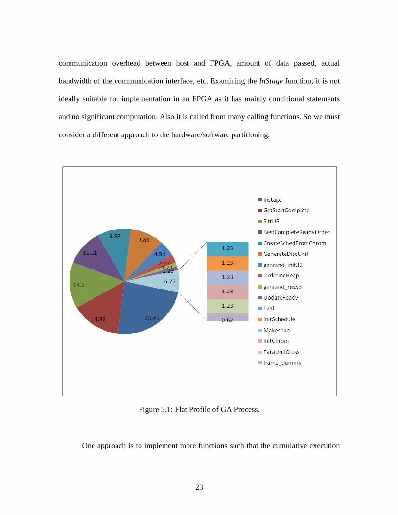
partitioning. The flat profile data for the GA application is shown in the pie-chart in
Figure 3.1. The profile data looks challenging for hardware acceleration as it is not
concentrated in a single (or few) function(s) that largely dominate the execution time,
making the hardware/software partitioning decision difficult. The most time consuming
function in the GA is InStage (23.46%), which checks if a specific job has entered any of
the stages of the flow-line. Based on Amdahl’s law [16], we can state that the speedup of
an application is limited by the portion of the program not being parallelized. So if we go
by the rule of thumb, that is implementing the regions that contribute to the highest
execution time, the maximum theoretical speedup we can achieve is:
Speedup= 1/(1-p) ................(5)
= 1/(1-0.2346)
= 1/0.7654
= 1.3X
Here, p is the portion of the code that is implemented in hardware and therefore
parallelized. To find the maximum speedup, we assume infinite parallelism by
implementing a code snippet in hardware. We see that even with these assumptions, the
speedup is insignificant. Also there are other significant constraints when functions are
implemented in hardware. For example, topology of the call graph to the function,
23
communication overhead between host and FPGA, amount of data passed, actual
bandwidth of the communication interface, etc. Examining the InStage function, it is not
ideally suitable for implementation in an FPGA as it has mainly conditional statements
and no significant computation. Also it is called from many calling functions. So we must
consider a different approach to the hardware/software partitioning.
Figure 3.1: Flat Profile of GA Process.
One approach is to implement more functions such that the cumulative execution

24
time of all the functions implemented in FPGA is closer to 80%. In that case, we can
expect a theoretical speedup of 5X according to eq. (5). But this partition exposes some
practical limitations mainly due to the topology of the call graph. Figure 3.2 shows a snap
shot of the overall call graph of the GA process. Figures 3.3 and 3.4 are the two
alternative partitions we evaluated.
Figure 3.2: Snap Shot of the Overall Call Graph

25
Figure 3.3: Call Graph for 1st Partition Evaluation
Figure 3.4: Call Graph for 2nd Partition Evaluation

26
InSatge, SiftUp, GenerateDiscUnif, BestCompleteReadyOrder, GetStartComplete,
and CreateSchedFromChrom is a set of functions that have a cumulative execution time
of 83.35%. As evident from Figure 3.3, the biggest disadvantage of the GA code for
hardware implementation is that functions are called from many different places and
many times. So if we want to implement a function in an FPGA by minimizing the host–
to–FPGA communication overhead, we need to implement at least some of its
predecessors. A call graph of this nature exposes additional problems. For example, even
if a function is suitable for implementation in an FPGA, its predecessor may not be. The
predecessors may have many conditional and branch statements. These statements are
very ill suited for FPGAs as FPGAs do not have branch prediction units whereas general
purpose microprocessors are equipped with efficient branch prediction units. Also if we
continue to implement the predecessors in the FPGA, at some point we will run out of
resources. These characteristics of the existing GA implementation make the
hardware/software partitioning more difficult. Especially the coarse-grained partitioning
is very hard in this case. As mentioned before, the fine-grained partitioning is not
intuitive. Considering these issues, we have implemented the basic GA operations
(Initchrom, ParaUnifCross and Immigrate as shown in Figure 3.4) in the FPGA. In
Figure 3.2, 3.3 and 3.4, the numbers above each function indicate the number of times it
is called by its calling function. Our implementation follows a coarse-grained partitioning
as we partition based on the functions.
The partition evaluation approach we have followed is based on an estimation of
the overall application performance with the constraint of using one user FPGA. We
27
consider the cumulative execution time of the functions implemented in the FPGA, the
amount of data passed to and from the FPGA, and the resources they consume as our
estimation criteria. We have only explored the two possibilities shown in the two call
graphs of Figure 3.3 and 3.4 and decided to go on with Figure 3.4. As Figure 3.4
incorporates the basic GA functions, it supports our claim of an implementation of the
GA in an FPGA. Also the call graph associated with these GA operations is more
contained than the call graph of Figure 3.3, minimizing the host-to-FPGA communication
overhead.
Our implementation uses only one FPGA for two reasons. First, as we are using
coarse-grained partitioning, there is less opportunity for inter-partition communication, so
it is very unlikely that the computation result of one PE will be used by another.
Therefore even if we chose to use more than one FPGA, it is highly probable that the
results of one FPGA are not needed by the second one. In that case, the second FPGA
depends on the data passed to it by the host which has higher communication cost than
data passed from the first FPGA. Secondly, the more functions we implement in FPGA,
the more complicated the overall application call tree becomes. Because of these factors,
we have only implemented those functions in the FPGA that account for a cumulative
execution time of 2.46%. Therefore the maximum theoretical speedup we can expect
according to eq. (5) is 1.025X.

28
3.2 Systems and Tools Used
Our implementation was developed in a 2GHz Intel Xeon CPU populated with 2
Nallatech H101 PCI-XM FPGA accelerator boards. The specification [17] of this board is
as follows:
• 1 user FPGA – Virtex 4 LX100 (XC4VLX100-10FF1148C)
• 4 banks of DDR2 SSRAM
o Each has 4MB of memory, totaling 16 MB
o Total bandwidth: 6.4GB/s
• 1 bank of DDR2 SDRAM
o 512MB of memory
o Bandwidth: 3.2GB/s
• 4 channel serial communication (board-to-board)
o Bandwidth: 2.5 Gb/s
o Latency: 340 ns
• PCI-X connectivity with host
o 64-bit, 133MHz
Figure 3.5 shows the functional diagram of H101-PCIXM [17].

29
Figure 3.5: Functional Diagram of H101 PCI-XM
During the development process, we used DIME-C [18] which is a high-level
language, rather than a hardware description language such as VHDL or Verilog. DIME-
C [18] is a subset of ANSI-C and provides the programmer with the flexibility of writing
code for the FPGA without having to focus on the hardware in detail. DIME-C compiles
code to VHDL automatically. This VHDL module is then used as a Processing Element
(PE) that works inside an FPGA. Then we use DIMETalk [19], a tool for designing the
network that interfaces with the host. DIMETalk defines how the PEs are connected to
30
other on-chip or on-board resources. Using DIMETalk, we generate the bitstream and the
sample host code to be used in the host application. The host code is then modified
according to the application and the data that must be transferred. The host code is
responsible for reading from and writing to the FPGA, switching on and off the FPGA,
and other housekeeping operations.
3.3 Implementation Models
We will discuss four methods that comprise our implementation model. The methods
are:
• Communication Methods
• Execution Methods
• Implementation Methods
• Configuration Methods
The Reconfigurable Processing Fabric (RPF), or FPGA, is used as a coprocessor in
our system. Figure 3.6 shows the location of FPGA in the memory hierarchy.
31
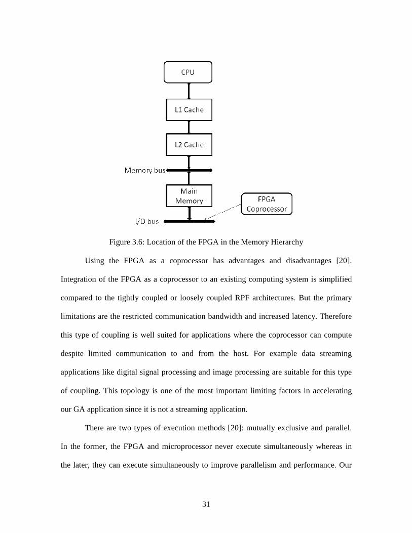
Figure 3.6: Location of the FPGA in the Memory Hierarchy
Using the FPGA as a coprocessor has advantages and disadvantages [20].
Integration of the FPGA as a coprocessor to an existing computing system is simplified
compared to the tightly coupled or loosely coupled RPF architectures. But the primary
limitations are the restricted communication bandwidth and increased latency. Therefore
this type of coupling is well suited for applications where the coprocessor can compute
despite limited communication to and from the host. For example data streaming
applications like digital signal processing and image processing are suitable for this type
of coupling. This topology is one of the most important limiting factors in accelerating
our GA application since it is not a streaming application.
There are two types of execution methods [20]: mutually exclusive and parallel.
In the former, the FPGA and microprocessor never execute simultaneously whereas in
the later, they can execute simultaneously to improve parallelism and performance. Our

32
implementation model is mutually exclusive, which also limits the achievable
performance of the overall GA application. One advantage of the mutually exclusive
execution method is that it makes the partition evaluation estimation easier. But in this
case we are only exploring a few hardware/software partitions.
Implementation methods are of two types: separate datapath and fused datapath.
In separate datapath, the flow of data is independent whereas in fused, the paths are fused
to reduce the area overhead. Although in the fused datapath approach, the performance
may suffer due to a longer circuit path. As we are using a high-level language to program
the FPGA, we do not have control over these methods. Whether our implementation will
use separate or fused datapaths depends on the FPGA platforms and tools we are using.
Dynamic reconfiguration and partial runtime reconfiguration are two
configuration methods that increase the effective size of the FPGAs. Dynamic
reconfiguration allows tasks to be time shared [21]. We do not use this feature as the
logic resources are not the main limiting factor in our approach. Partial runtime
reconfiguration allows configuration of a portion of the FPGA while other portions
continue to operate. This approach can improve performance as it can execute code in a
portion of the FPGA without interrupting the other segments of the FPGA that are
running. But this feature is generally not supported in currently available high-
performance RC systems.
3.4 Accelerating State Vector Generation
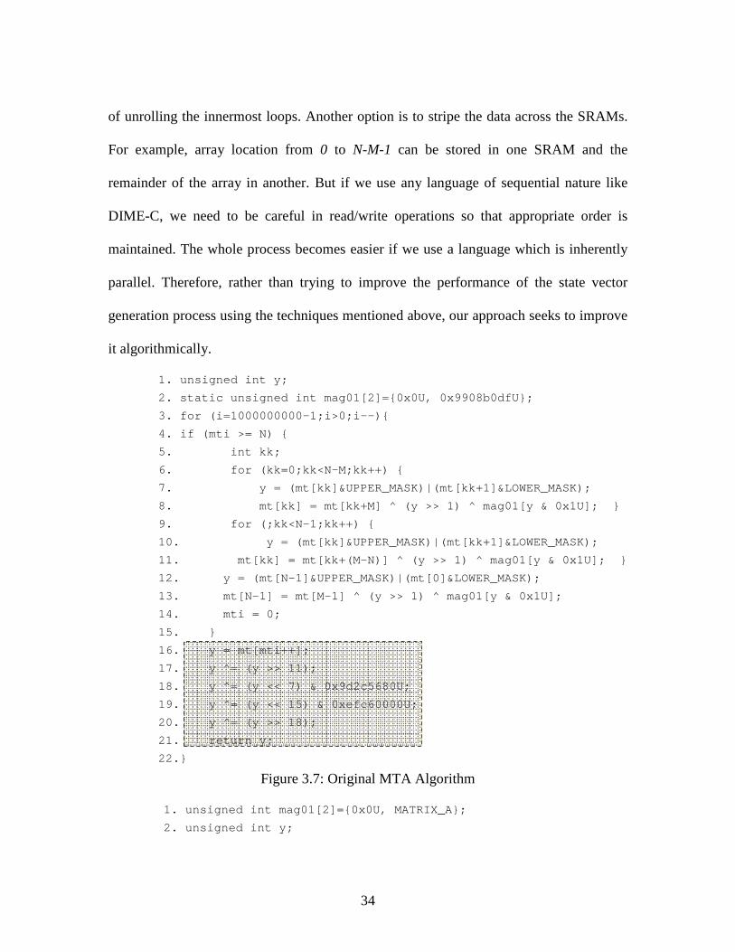
The original MTA algorithm is shown in Figure 3.7. For generating state vectors,

33
this algorithm iterates one billion times since we are saving state vectors at intervals of
one billion numbers. That is why there is an outer loop (line 3 of Figure 3.7) that iterates
one billion times. This outer loop limits the performance in the FPGA implementation
since DIME-C can only unroll the innermost loop. Even with the two innermost loops
(lines 6 and 9 shown in Figure 3.7), there are challenges in finding and exploiting
parallelism. The primary limitation is the memory access pattern of the MTA algorithm.
Inside the for-loop, the same location of mt array is read and written back. This array is
an input to the FPGA passed from the host. In our implementation, we use BRAM to
store that array. Therefore according to the DIME-C specification [18], an array stored in
a BRAM is passed to the PE module. For this reason, even if the BRAMs are dual ported,
the consecutive read/write inside the for-loop cannot occur in the same cycle. So even if
the two for loops in Figure 3.7 are the innermost loops, they cannot be fully unrolled as
they would violate this condition. As a result, these two innermost loops cannot be
pipelined. Since we loop through the code body one billion times, this overhead is
multiplied and causes poor performance of the MTA algorithm in the FPGA.
To avoid the problems associated with the memory access pattern, there are a
couple of options to consider. Instead of using BRAM to store the data, one option is to
use SRAM. We have four banks of SRAM available in the system. Data can be
duplicated in those banks allowing read and write to the same location in different
memory banks. This option, while it enables the loop unrolling, has the associated
overhead of copying the modified mt back to the SRAM before the next iteration of the
outermost loop. Performing this copy operation one billion times outweighs the benefits
34
of unrolling the innermost loops. Another option is to stripe the data across the SRAMs.
For example, array location from 0 to N-M-1 can be stored in one SRAM and the
remainder of the array in another. But if we use any language of sequential nature like
DIME-C, we need to be careful in read/write operations so that appropriate order is
maintained. The whole process becomes easier if we use a language which is inherently
parallel. Therefore, rather than trying to improve the performance of the state vector
generation process using the techniques mentioned above, our approach seeks to improve
it algorithmically.
1. unsigned int y;
2. static unsigned int mag01[2]={0x0U, 0x9908b0dfU};
3. for (i=1000000000-1;i>0;i--){
4. if (mti >= N) {
5. int kk;
6. for (kk=0;kk<N-M;kk++) {
7. y = (mt[kk]&UPPER_MASK)|(mt[kk+1]&LOWER_MASK);
8. mt[kk] = mt[kk+M] ^ (y >> 1) ^ mag01[y & 0x1U]; }
9. for (;kk<N-1;kk++) {
10. y = (mt[kk]&UPPER_MASK)|(mt[kk+1]&LOWER_MASK);
11. mt[kk] = mt[kk+(M-N)] ^ (y >> 1) ^ mag01[y & 0x1U]; }
12. y = (mt[N-1]&UPPER_MASK)|(mt[0]&LOWER_MASK);
13. mt[N-1] = mt[M-1] ^ (y >> 1) ^ mag01[y & 0x1U];
14. mti = 0;
15. }
16. y = mt[mti++];
17. y ^= (y >> 11);
18. y ^= (y << 7) & 0x9d2c5680U;
19. y ^= (y << 15) & 0xefc60000U;
20. y ^= (y >> 18);
21. return y;
22.}
Figure 3.7: Original MTA Algorithm
1. unsigned int mag01[2]={0x0U, MATRIX_A};
2. unsigned int y;
35
3. int kk, I, if1=0, if2=0, else1=0, flag=0;
4. for(i=1000000000-1; i>0;i--){
5. if (mti>=N){
6. flag=1;
7. for (kk=0;kk<N-M;kk++) {
8. y= (mt[kk]&UPPER_MASK)|(mt[kk+1]&LOWER_MASK);
9. mt[kk] = mt[kk+M] ^ (y >> 1) ^ mag01[y & 0x1U];}
10. for (kk=N-M;kk<N-1;kk++) {
11. y = (mt[kk]&UPPER_MASK)|(mt[kk+1]&LOWER_MASK);
12. mt[kk] = mt[kk+(M-N)] ^ (y >> 1) ^ mag01[y & 0x1U];}
13. y= (mt[N-1]&UPPER_MASK)|(mt[0]&LOWER_MASK);
14. mt[N-1] = mt[M-1] ^ (y >> 1) ^ mag01[y & 0x1U];
15. if(i-624>=0){
16. mti=624;
17. i=i-623; }
18. else{
19. mti=i;
20. i=1;}
21. }
22. else if( mti<624 && flag==0) {
23. flag=1;
24. i=i-(624-mti)+1;
25. mti=624;}
26.}
Figure 3.8: Improved MTA for State Vector Generation
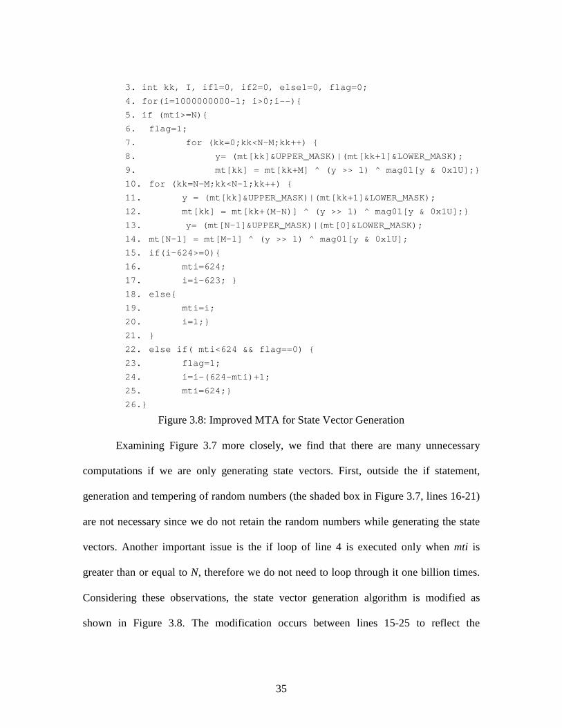
Examining Figure 3.7 more closely, we find that there are many unnecessary
computations if we are only generating state vectors. First, outside the if statement,
generation and tempering of random numbers (the shaded box in Figure 3.7, lines 16-21)
are not necessary since we do not retain the random numbers while generating the state
vectors. Another important issue is the if loop of line 4 is executed only when mti is
greater than or equal to N, therefore we do not need to loop through it one billion times.
Considering these observations, the state vector generation algorithm is modified as
shown in Figure 3.8. The modification occurs between lines 15-25 to reflect the
36
observations mentioned above.
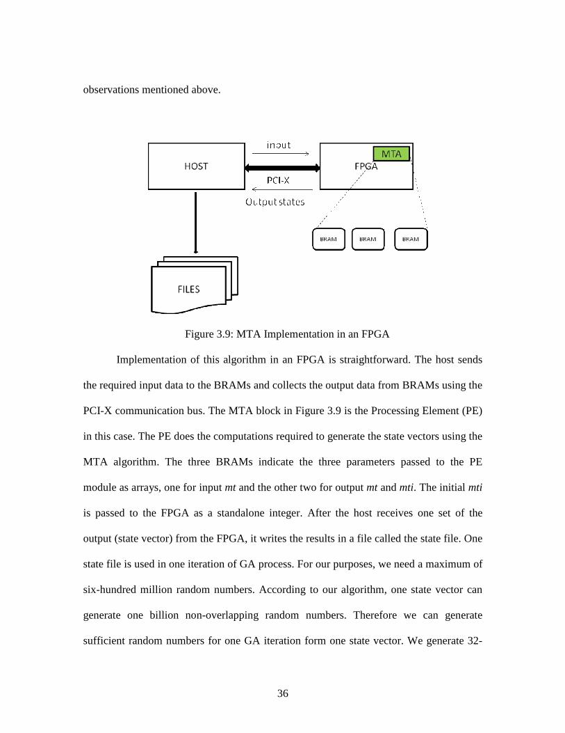
Figure 3.9: MTA Implementation in an FPGA
Implementation of this algorithm in an FPGA is straightforward. The host sends
the required input data to the BRAMs and collects the output data from BRAMs using the
PCI-X communication bus. The MTA block in Figure 3.9 is the Processing Element (PE)
in this case. The PE does the computations required to generate the state vectors using the
MTA algorithm. The three BRAMs indicate the three parameters passed to the PE
module as arrays, one for input mt and the other two for output mt and mti. The initial mti
is passed to the FPGA as a standalone integer. After the host receives one set of the
output (state vector) from the FPGA, it writes the results in a file called the state file. One
state file is used in one iteration of GA process. For our purposes, we need a maximum of
six-hundred million random numbers. According to our algorithm, one state vector can
generate one billion non-overlapping random numbers. Therefore we can generate
sufficient random numbers for one GA iteration form one state vector. We generate 32-

37
bit unsigned integers as the state vectors though the flow-line scheduling research used
64-bit unsigned long numbers. This smaller data type is used because DIME-C does not
support long integers. A workaround for generating 64-bit state vectors will be discussed
in section 3.6.
3.5 Implementing Genetic Algorithm in FPGA
The design of the basic GA functions for FPGA implementation is similar to the
MTA implementation in the sense that the current implementation of the GA only uses
BRAMs, no external memory. First, the amount of data is small enough to fit in the
BRAMs and second the GA is not a streaming application. The basic block diagram of
the design used to implement the core GA functions is shown in Figure 3.10. Three PEs
are implemented in the FPGA that correspond to the four main operations of GA. Each of
the PEs requires random numbers that are generated using the previously saved state
vectors. In our implementation, we generate the random numbers inside each of the PEs
as they are required. In our implementation, different PEs are called from the host at
different times. As each of the PEs generate random numbers from the state vector inside
the FPGA, the mti value is updated inside them. The mti value along with the mt array is
always passed back to the host from the PEs so that in the next call to PEs, the updated
ones are used.
The PE labeled InitChrom initializes the population. In our implementation, the
size of the population is 100, i.e. the population consists of 100 chromosomes. Each of
the chromosomes is initialized with random gene values. These gene values are double-
38
precision floating-point numbers. The PE labeled ParaUnifCross works on selection and
crossover steps of the GA. Therefore this PE needs data for all of the chromosomes.
Random parents are selected for the crossover operation along with the random crossover
point. After the crossover, the successors are generated, i.e. gene values of the
chromosomes are updated. These updated values are passed back to the host to be used in
other required computations of the flow-line scheduling problem. The PE labeled
Immigrate performs the immigration operation discussed in section 2.1.1. The starting
point of the immigration along with the gene values are the inputs to the PE. The gene
values of the chromosomes are updated during immigration and passed back to the host
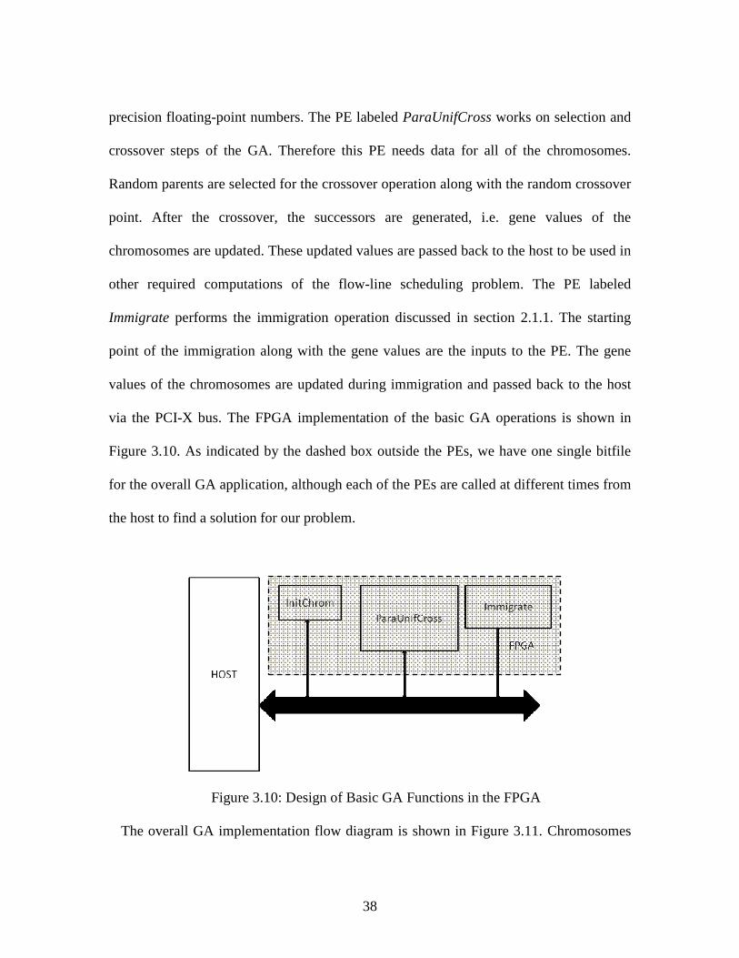
via the PCI-X bus. The FPGA implementation of the basic GA operations is shown in
Figure 3.10. As indicated by the dashed box outside the PEs, we have one single bitfile
for the overall GA application, although each of the PEs are called at different times from
the host to find a solution for our problem.
Figure 3.10: Design of Basic GA Functions in the FPGA
The overall GA implementation flow diagram is shown in Figure 3.11. Chromosomes

39
are initialized randomly. These chromosomes are then evaluated in host to see if it
satisfies the optimization criteria. If not then the next three steps of the GA starts
executing in the FPGA - selection of qualified parents for generating a better successor,
crossover to produce the successor, and mutation (replaced by immigration in this
implementation) to increase the fitness of the successor.
Figure 3.11: Flow-Chart of the Overall GA Implementation
3.6 Limitations of Our Design
Since the GA is not a streaming application, it is not ideally suited for our system
(where FPGA is a coprocessor) as discussed in section 3.3. There are a couple of options
that can potentially improve the performance within the constraints of the system and
tools. Our current design does not consider those options, but they are discussed below
with justifications for not supporting them.
The original GA implementation for solving the flow-line scheduling problem
was targeted for a general-purpose microprocessor. We take pieces of that code to
implement in a FPGA based on profile data. This approach limits the overall performance

40
of the FPGA implementation as the original implementation never considered a
specialized architecture. The topology of the call graph indicates a significant amount of
communication overhead between the basic GA processes and other modules of the flow-
line scheduling implementation. This communication overhead, though insignificant for a
general-purpose microprocessor, is a limiting factor in an FPGA implementation. This
bottleneck in performance results from the hardware/software partition, which separates
the basic GA operations in the FPGA implementation from the overall application
running in the host. That means, if we do not consider redesigning the application
targeting the FPGA, we have to pay the price for communication overhead between the
host and the FPGA. Therefore while targeting this application for the FPGA
implementation, better performance is possible if the entire application were redesigned
specifically for an FPGA-based platform.
We improved the state vector generation process algorithmically, but we have not
incorporated the suggested memory access pattern discussed in section 3.4, which could
further improve performance.
An important design strategy of most FPGA implementations is passing data to
and from FPGA only when it is absolutely necessary. It is crucial to move data judicially
as the corresponding overheads are significant. In our design, we pass data back to host
whenever we have enough results for creating one state file. Though it does not have a
significant impact for generating one state file, it has a cumulative impact on how quickly
we can generate multiple state files.
Using a C-like programming language (such as DIME-C), though has the

41
advantage of higher productivity from the programmer’s point of view, makes it harder to
take full advantage of the FPGA. Since DIME-C is still sequential in nature, the
programmer needs to code explicitly to take advantage of the inherent parallelism of an
FPGA. Conversely, as VHDL is inherently parallel, it is easier to exploit the parallelism
of an FPGA.
The biggest disadvantage of this design comes when we consider the design of the
GA algorithm in the FPGA. The random number generation is independent of the basic
GA operations since they are produced from the previously generated state files, using
variables that are independent of the basic GA operations. But we are not fully taking
advantage of this available parallelism. Using the MTA algorithm and the previously
generated state vectors, random numbers can be generated and stored in a FIFO from
where these GA operators can access them as needed. This concept is shown in Figure
3.12. Our current implementation does not incorporate this approach and is considered
for future work.
Figure 3.12: Random Number Generation in Parallel Using a FIFO

42
3.7 Summary
Our design and implementation techniques achieve a performance gain in the
state vector generation but performance decreases in the overall GA process. Chapter 4
discusses the results and analyzes them within the constraints of the RC systems and tools
used.

43
CHAPTER 4
PERFORMANCE AND RESULT ANALYSIS
This chapter presents and analyzes the performance results from the system’s
perspective: the underlying hardware architecture, memory hierarchy, and
communication interface. We also discuss how the algorithm interacts with the system
and impacts the final results and performance.
4.1 Performance Improvement of State Vector Generation
Compared to the original implementation, the improved MTA algorithm for state
vector generation, introduced in Chapter 3, performs 5X faster in the general-purpose
microprocessor and 2.4 times faster than its original in the FPGA implementation. The
original FPGA implementation executes at a clock frequency of 139MHz while the
improved one runs at 157MHz. The clock frequency increase is due to the improvement
in the algorithm. As shown in Figure 3.8, the improved algorithm does not iterate one
billion times through the code body. Therefore it does not access the state vector array
and the random numbers that many times. As a result, outputs are generated with fewer
memory accesses resulting in a higher clock frequency. Table 4.1 shows a summary of
the performance data of state vector generation algorithm.

44
Table 4.1: Performance Data of State Vector Generation Using MTA Algorithm
Property Original
Algorithm
Improved
Algorithm
Improvement
S/W time for one state file
( microprocessor)
45.3 sec 9 sec 5.03X
S/W time for one state file
(FPGA implementation)
350 sec 146.44 sec 2.4X
H/W Cycles 12,724,078 9,892,294 1.488X
An important point to note from Table 4.1 is that the improved algorithm has about
5X speedup over its original general-purpose microprocessor implementation while only
about 2.4X speedup in the FPGA implementation. The improved algorithm of Figure 3.8
has more conditional statements than the original, which is suitable for the von Neumann
architecture but not ideal for an FPGA. As general-purpose microprocessors are equipped
with efficient branch prediction units, efficient execution of the improved algorithm is
not a problem. Since FPGAs do not have similar branch prediction units, a significant
performance bottleneck results while executing conditional and branch statements.
Without these branch prediction units, FPGAs may implement all the cases of conditional
statements in the data path to improve performance. Whenever a conditional statement
occurs, assessing that condition requires extra cycles that are not necessary in a general-
purpose microprocessor. For most modern microprocessors, the branch prediction
accuracy is more than 95%; meaning, in 95% cases, they do not execute the conditional
45
statements. They can safely assume the prediction result from Prediction History Table
(PHT), a table where the previous conditional statement check results are stored. Based
on the results of PHT, they move to the later stages of instruction execution. Only in less
than 5% of the cases, the miss-prediction occurs and requires extra cycles to bring the
proper set of instructions in the pipeline stages. As general-purpose microprocessors
typically run 10X to 20X faster than FPGAs, the miss-prediction penalty of extra cycles
is insignificant. In our design, the FPGA runs at around 15X slower clock frequency than
the microprocessor. The cumulative effect of these issues results in the poor performance
of an FPGA while executing conditional and branch statements.
Another important issue is the potential increase in area overhead when conditional
statements are implemented in FPGAs. In lieu of branch prediction units, FPGAs can
implement both data path conditions increasing the area requirement.
The number of hardware cycles required in the improved algorithm implementation is
9,892,294 whereas the original implementation requires 14,724,078 cycles, a 1.488X
improvement. The hardware cycle count only considers the cycles required for an
algorithm to execute in the FPGA. Whereas the runtimes discussed before also include
the data transfers and other communication. 19.5KB of data is passed between the host
and the FPGA and the communication overhead is 16 microseconds.
We use the following terms to define speedup of an algorithm in an FPGA compared
to its general-purpose microprocessor implementation:
S CPU clock cycles
H Hardware (FPGA in this case) cycles

46
F FPGA clock frequency
M Microprocessor clock frequency
M
F
H
SSpeedup ×= (6)
For our system, M is 2 GHz.
For the original algorithm, F = 139 MHz, H= 12,724,078 cycles and for the improved
algorithm, F=157 MHz, H=9,892,294 cycles. To calculate S, we will use eq. (7).
CPU clock cycles = CPU execution time x Clock frequency (7)
CPU execution time is 45.3 sec for the original and 9 sec for the improved algorithm.
Clock frequency is 2GHz. Therefore using eq. (7), S for original and improved algorithm
are 45,300,000,000 cycles and 9,000,000,000 cycles respectively. Now using eq. (6), the
speedup for the original algorithm in the FPGA implementation is 494.87X. The FPGA
implementation of the original algorithm runs 494.87X faster than the general-purpose
microprocessor if we consider the fact that the clock frequency of the FPGA is about 20X
(in our design 14.388X) slower than the microprocessor. Conversely, the normalized
speedup for the improved algorithm is 142.84X in the FPGA implementation. Even
though the improved design runs at a higher clock frequency (157MHz), the performance
is lower than the speedup of the original algorithm. As previously mentioned, the
improved algorithm (improved for the microprocessor implementation) is not well suited
for an FPGA as it has several conditional statements. Therefore the number of hardware
cycles is not low enough to raise the speedup value based on eq. (6).
The resource utilization for both the original and improved algorithms are shown in
Table 4.2. As compared to the other resources, the LUT requirement is significantly

47
reduced (30.44%) for the improved algorithm. Referring to the algorithm shown in Figure
3.8, the reduction in resource utilization results from not performing the random number
tempering on the variable y. In other words, we are using the variable y fewer times than
in the original algorithm of Figure 3.7 contributing to this reduction in the resource
requirements.
Table 4.2: Resource Utilization of State Vector Generation Algorithm
Resource
name
Original
algorithm
Improved
algorithm
% resource reduction
BRAMs 51/240 (21%) 37/240 (15%) 27.45%
Slices 5451/49152
(11%)
4124/49152
(8%)
24.34%
4-input LUTs 8351/98304
(8%)
5809/98304
(5%)
30.44%
Both implementations pass 19.5KB of data between host and FPGAs through the
PCI-X bus. This PCI-X bus is capable of passing 64-bit data with a maximum of
133MHz theoretical speed [24]. Therefore the maximum data transfer rate is 8.3125Gb/s.
This data transfer rate is the theoretical rate and the effective rate is actually lower due to
the overhead and other system design tradeoffs. The overheads include data transfer
overhead, transaction layer packet overhead, flow control overhead, etc. [25].
Considering these factors, the sustainable host bandwidth is 400 MB/s [24]. As the data

48
passed between the host and FPGA is only about 19.5KB for one state file, the
communication overhead is insignificant, i.e. 16 microseconds to be specific. But
considering that we must generate many state files, this overhead can be significant. For
example, the flow line scheduling requires generating 360K state files. With 16
microsecond communication overhead per file, the cumulative overhead is 5.76 seconds
for all 360K files. One possible improvement of this design would be to store state
vectors in on-board memory (like SRAM) and send them at set intervals or at the
conclusion of the file generation taking maximum advantage of the PCI-X bus
bandwidth. This approach will require analysis of the tradeoff between SRAM size and
PCI-X bus bandwidth and when it is most efficient to send data back to the host. As the
size of each SRAM is 4MB and the size of one state file is 20KB (625 unsigned integers),
we can store a maximum of 200K state files in a SRAM. But the time to generate 4MB
data is too long. With our improved algorithm, the generation of 4MB data will require
about 339 days (200K files, each with 146.44 seconds). That means, if results are
returned to the host once the SRAM is filled up, the user will have to wait for 339 days
before she can see the first state file. Therefore there should be a tradeoff between the
maximal use of PCI-X bandwidth and throughput rate based on the application
requirement.

49
4.2 GA Performance Analysis
In this section we discuss the implementation results and performance of basic GA
operations. Table 4.3 shows the performance results of each of the PEs of the GA
process.
Table 4.3: Performance Data of Basic GA Operations.
Property InitChrom ParaUnifCross Immigrate
S/W time
(general-purpose microprocessor)
50 micro sec. 0.17 sec. 50 micro sec.
Total time (FPGA) 100 micro sec 1.21 sec. 100 micro sec.
H/W Cycles 1612 3123 1116
FPGA design frequency 101.871MHz 130.162MHz 101.871MHz
As seen in the table, the InitChrom and Immigrate modules run 2X slower in the FPGA
than the general-purpose microprocessor whereas ParaUnifCross runs 7.12X slower. The
values of S for these three modules are 50, 170 and 50 cycles respectively. Therefore, the
speedup for InitChrom, ParaUnifCross and Immigrate based on eq. (6) are 1.58x10⁻³,
2.28x10⁻³ and 3.54x10⁻³ respectively.
Even with the function by function comparison, the FPGA implementation is much less
efficient as shown in the execution time comparison. This inefficiency occurs because the
implementation of basic GA operations is not well suited for a FPGA. The reasons can be
explained by analyzing the pseudocode in Figure 4.1.

50
1. void InitChrom(struct chrom *Chrom, struct data *PD) {
2. int j;
3. for (j=1; j<Chrom->numjobs; j++) {
4. if (InStage(PD, j, 0)) {
5. Chrom->StageChroms.keys[j]=GenerateDiscUnif(0,Chrom-
>StageChroms.nummcs - 1);
6. Chrom->StageChroms.keys[j]=Chrom-
>StageChroms.keys[j]*(int)pow(10,Chrom->places);
7. Chrom->StageChroms.keys[j]=Chrom-
>StageChroms.keys[j]+GenerateDiscUnif(1, (int)pow(10,Chrom-
>places)-1);
8. }
9. else Chrom->StageChroms.keys[j]=0;
10. }
11. Chrom->changed=TRUE;
12.}
Figure 4.1: Initchrom Function in General-Purpose Microprocessor
As shown in lines 4, 5 and 7 of Figure 4.1, different functions are called from this
function with different parameters to initialize the chromosome. The InStage function is
called with different parameters for each iteration. The GenerateDiscUnif function calls
the random number generation process. Even with the in-lining of those functions, code
of this nature is not ideally suited for an FPGA implementation. Also the if-else
conditions of lines 4 and 9 add to the inefficiencies as discussed earlier. One possible
improvement is to execute the InStage function independent of this code segment and
store the results in a FIFO. In that case, this code segment can simply read the values
from the FIFO and proceed.
If we want performance improvement of an application implemented in an FPGA
verses its microprocessor counterpart, the algorithm should have some characteristics that
will facilitate exploiting the architectural benefits of an FPGA. They are discussed below.

51
The algorithm should have some options for exploiting the inherent parallelism of an
FPGA. This feature includes independent memory access, options for loop unrolling and
loop flattening, independent tasks, etc. Even if the algorithm does not have these inherent
characteristics, there should be options available to modify the application to fit to those
features. This application is limited in this regard mainly because of the topology of the
call graph. The topology led us to a coarse-grained partitioning whereas in most of the
cases it would be better if we could do fine-grained partitioning. But fine-grained
partitioning would make the partition combination tougher since the functions are called
from many different places, and likely their combination overhead would not perform
better.
Related to the previous point, an important question is whether the implementation
suits the target architecture or not. As discussed in section 4.1, the existence of
conditional and branch statements here in the GA process is a bottleneck for performance
improvement. The call graph of this algorithm readily reveals the fact that there is
significant jumping from one function to another adding to the probability of a
performance bottleneck for an FPGA implementation.
Another point is whether the application is streaming or not. As we are using the FPGA
as an independent coprocessor, having a streaming application would improve the
chances of application acceleration. The GA fails here as it is not a streaming application.
For hardware/software partitioning, we chose coarse-grained partitioning. An important
question is whether the fine-grained partitioning would help us in any way for the
functions we chose to implement in the FPGA. Examining Figure 4.2, we conclude that
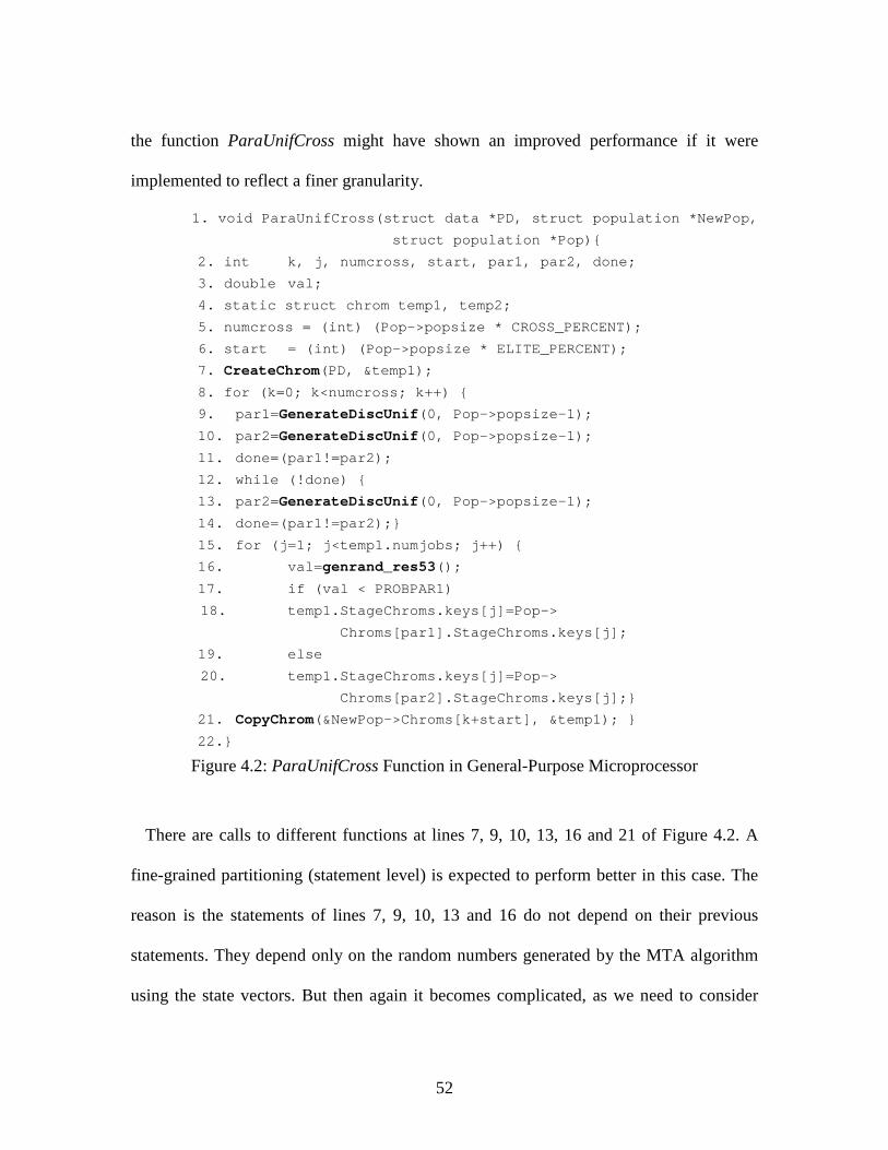
52
the function ParaUnifCross might have shown an improved performance if it were
implemented to reflect a finer granularity.
1. void ParaUnifCross(struct data *PD, struct population *NewPop,
struct population *Pop){
2. int k, j, numcross, start, par1, par2, done;
3. double val;
4. static struct chrom temp1, temp2;
5. numcross = (int) (Pop->popsize * CROSS_PERCENT);
6. start = (int) (Pop->popsize * ELITE_PERCENT);
7. CreateChrom(PD, &temp1);
8. for (k=0; k<numcross; k++) {
9. par1=GenerateDiscUnif(0, Pop->popsize-1);
10. par2=GenerateDiscUnif(0, Pop->popsize-1);
11. done=(par1!=par2);
12. while (!done) {
13. par2=GenerateDiscUnif(0, Pop->popsize-1);
14. done=(par1!=par2);}
15. for (j=1; j<temp1.numjobs; j++) {
16. val=genrand_res53();
17. if (val < PROBPAR1)
18. temp1.StageChroms.keys[j]=Pop->
Chroms[par1].StageChroms.keys[j];
19. else
20. temp1.StageChroms.keys[j]=Pop->
Chroms[par2].StageChroms.keys[j];}
21. CopyChrom(&NewPop->Chroms[k+start], &temp1); }
22.}
Figure 4.2: ParaUnifCross Function in General-Purpose Microprocessor
There are calls to different functions at lines 7, 9, 10, 13, 16 and 21 of Figure 4.2. A
fine-grained partitioning (statement level) is expected to perform better in this case. The
reason is the statements of lines 7, 9, 10, 13 and 16 do not depend on their previous
statements. They depend only on the random numbers generated by the MTA algorithm
using the state vectors. But then again it becomes complicated, as we need to consider

53
integrating it with the overall GA process and eventually with the flow-line scheduling
application.
These reasons add to the inefficient runtime of the GA operators compared to its von
Neumann counterpart. But an improved design as shown in Figure 3.12 is expected to
improve the performance compared to the current FPGA implementation as in Figure
3.10.
Resource utilization for GA operators (individual resource consumption of PEs) is
shown in Table 4.4. It is evident that the ParaUnifCross PE is consuming most of the
FPGA resources. ParaUnifCross is actually a combination of selection and crossover
operations of the GA so it has much more computation compared to the other PEs
currently implemented. The overall resource utilization is almost equal to 100%. An
important point to note is that in our current implementation, all the GA operations
generate random numbers inside their own module. This approach actually increases the
resource requirement. If the implementation reflects the design of Figure 3.12, we can
eliminate the need for a random number generator per PE and thereby reduce the resource
utilization.
Table 4.4: Resource Utilization of GA Operations.
Resource Name Initchrom ParaUnifCross Immigrate
BRAMs 54/240 (22%) 109/240 (45%) 54/240 (22%)
Slices 13,397/49152 (27%) 17890/49152 (36%) 13,428/49152 (27%)
4-input LUTS 18,592/98304 (18%) 27341/98304 (27%) 18,689/98304 (19%)
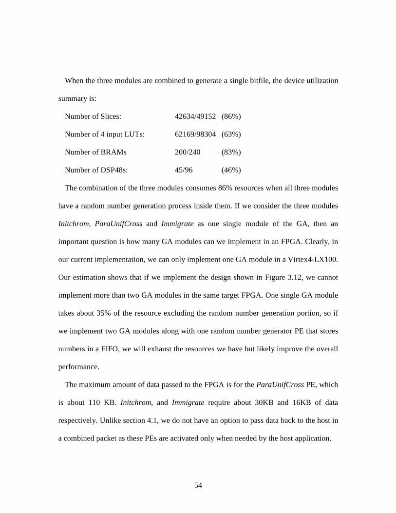
54
When the three modules are combined to generate a single bitfile, the device utilization
summary is:
Number of Slices: 42634/49152 (86%)
Number of 4 input LUTs: 62169/98304 (63%)
Number of BRAMs 200/240 (83%)
Number of DSP48s: 45/96 (46%)
The combination of the three modules consumes 86% resources when all three modules
have a random number generation process inside them. If we consider the three modules
Initchrom, ParaUnifCross and Immigrate as one single module of the GA, then an
important question is how many GA modules can we implement in an FPGA. Clearly, in
our current implementation, we can only implement one GA module in a Virtex4-LX100.
Our estimation shows that if we implement the design shown in Figure 3.12, we cannot
implement more than two GA modules in the same target FPGA. One single GA module
takes about 35% of the resource excluding the random number generation portion, so if
we implement two GA modules along with one random number generator PE that stores
numbers in a FIFO, we will exhaust the resources we have but likely improve the overall
performance.
The maximum amount of data passed to the FPGA is for the ParaUnifCross PE, which
is about 110 KB. Initchrom, and Immigrate require about 30KB and 16KB of data
respectively. Unlike section 4.1, we do not have an option to pass data back to the host in
a combined packet as these PEs are activated only when needed by the host application.

55
As discussed in section 3.1.2, the overall GA application speedup should ideally be
1.025X. But it is readily understandable that with the communication overhead and the
design problems discussed in section 4.2 and 3. 6, practically it would not be possible to
achieve any speedup.
For our research, we have two separate bitfiles for state vector generation and the GA.
Though the state vector generation is an initial step necessary for the operation of the GA,
we consider the GA our overall application. Therefore the resource utilization in the state
vector generation does not count towards the total resource utilization of the application.
If we consider the resource utilization from Table 4.2 and Table 4.4, we find that the total
percentage of BRAM usage is more than 100%. Since the bitfiles are separate and we do
not run them simultaneously, this is not a problem.
The results for our current implementation, though not impressive, open the door for
some interesting and seminal work in the future. We have exposed the issues and
understand the requirements necessary to design and implement a high-performance
computing application for a specialized architecture to gain maximum throughput within
the given constraints. We will discuss these in chapter 5.

56
CHAPTER 5
CONCLUSION AND FUTURE WORK
The focus of our work has been the acceleration of the GA in an FPGA. We have
shown that though there are challenges with the use of RC in scientific computing
applications like GAs, these challenges can be overcome when certain conditions are met.
Our contribution in this field is summarized in section 5.1. Later in section 5.2, we
discuss in detail the ideas for future work that will make RC a better fit for GAs.
5.1 Conclusion
We have presented an improved algorithm for state vector generation using MTA.
The algorithm eliminates some steps from MTA that are unnecessary for state vector
generation. Though there are potential approaches to improve performance by using the
FPGA resources more efficiently, the one billion iterations required before generating
one state vector limits the achievable performance of an FPGA implementation.
Therefore we chose to improve the performance by improving the algorithm. The
improved algorithm runs 5X faster in a general-purpose microprocessor than its previous
implementation and 2.4X faster in the FPGA than its previous FPGA implementation.
We have designed and implemented the basic GA operations in an FPGA. There
are four basic operations of the GA [5] and they are represented in three different PEs in
the FPGA. These three PE’s are combined to form a single GA module, meaning our
implementation has a single bitstream that represents the GA operations although the
three PE’s are called from the host at different times; there is only one active PE at any
given time during the FPGA execution. Each of the basic GA operation requires random

57
numbers for its operation. These random numbers are generated from the state vectors
inside each of the PEs. Our FPGA implementation of the GA runs about 7X slower than
its microprocessor counterpart for several reasons. The original GA implementation was
targeted for a general-purpose microprocessor and does not consider any specialized
architectures like FPGAs. Therefore the implementation is not ideal for an FPGA. We do
not design the application from scratch targeting our systems, rather we chose some
portion of the original implementation based on the profiling results and perform coarse-
grained partitioning to implement that in the FPGA. In some cases fine-grain partitioning
may perform better, but due to the topology of the call graph, it will not give us an overall
performance gain. Also we have not separated the random number generation process
from the basic GA operation, which is expected to improve performance in general and
allow for implementation of multiple GAs in a single FPGA. Overall, we have
inefficiencies in the FPGA implementation of the GA. The reasons are discussed in detail
in section 3.6, 4.1, and 4.2 along with suggestions for improvement.

58
5.2 Future Work
Possible future work involves both the state vector generation and the GA
implementations. First, we can implement the application in hardware description
languages (HDL) like VHDL or Verilog rather than using a high-level language (HLL)
like DIME-C. As HDLs are inherently parallel, we will need less attention to explicitly
specifying the parallelism in our implementation. As discussed in section 2.2, all previous
work on MTA and GA are in HDLs. One reason is that HDLs allow the designer to
exploit the parallelism of the FPGA in a more direct manner (not relying on the compiler
to infer the parallelism). Another interesting future direction would be a comparison
between the two implementation techniques: HDL and HLL. This comparison will show
us how the programming languages and their compilation techniques impact the
performance of an application targeted to a FPGA.
As discussed in section 3.6, the original implementation of the GA was targeted
for a von Neumann architecture with no consideration of an accelerator or specialized
hardware such as an FPGA-based RC platform. Most of the design constraints for our
approach relate to the inability to expose parallelism or compute density in the original
application. To exploit the parallelism of the RC system, we can design the application
from the scratch targeting the FPGA-based systems. The key consideration of that design
will be to reduce the communication overhead between the basic GA operations and
other portions of the application. Therefore the design should support calling the basic
GA module as few times as possible. In that case we will implement only the basic GA
operations in the FPGA and the host will use the outputs for other computations. To
59
reduce the host-to-FPGA communication overhead, we can perform GA operations on
the input data multiple times. This number will depend on the application and the host
can pass an upper limit of that number to the FPGA. When the output for the first GA
operation is available, the host can begin reading those results from the FPGA and
proceed with its computation while the FPGA is computing and storing the GA outputs in
an on-chip or on-board memory. This design would effectively support parallel execution
of the host and the FPGA. As soon as the stopping criterion is satisfied, i.e. the solution is
acceptable; the host will halt the execution of the FPGA. The reduced communication
overhead along with the parallel execution of the host and the FPGA will account for a
performance increase compared to our current implementation and most likely verses the
von Neumann counterpart as well. Once we have a GA module like the one described
above, we can use it to solve other optimization problems like placement and routing of
an FPGA and others that use a GA to find their solutions.
Our current implementation does not take advantage of overlapping
communication with computation. This limitation is a significant bottleneck for our
current implementation of the state vector generation. Also we need to incorporate this
overlapping if we want to implement the design techniques of Figure 3.12 or the
technique described in the paragraph above. To hide these data transfer overheads, we
could use on-board memories like SRAM or SDRAM or on-chip interfaces like FIFOs to
store data temporarily before the host reads them.
60
Another technique of parallelizing the state vector generation process is to stripe
data across memory banks so that at least some of the memory accesses, shown in Figure
3.8 (line 8, 9, 11 and 12) can happen simultaneously.
As discussed in section 3.6, allowing the random number generation to occur in
parallel with the GA process by incorporating a FIFO will improve the performance of
the application and is considered an important future direction.
Implementing the GA in other architectures like the Cell Broadband Engine (Cell
BE) or a Graphics Processing Unit (GPU) may be an interesting area to explore. Each of
these systems has its own advantages and disadvantages that may or may not suit an
application. GPUs are suitable for streaming applications. As GA is not a streaming
application, most likely we will not be able to achieve any significant performance gain
by implementing the GA in a GPU. On the other hand, the 6 different Synergistic
Processing Elements (SPE) of the Cell BE can be used to run 6 GA modules
independently, thereby extracting parallelism out of the multicore architecture of the Cell
BE.
Our future work also includes studying the behavior of a GA in a large-scale
cluster. The primary focus is to work on a large-scale cluster of FPGAs but a cluster of
Cell BE may also be considered once we have the implementation in one Cell BE. With
the growing number of computing resources, performance and scalability of the GA
implementation in these clusters are important metrics of analysis.
A relatively newer concept related to the GA is Evolvable Hardware (EH). The
concept of EH arises from the analogy between a living being and a circuit. The DNA

61
(deoxyribonucleic acid) of a living being is a string of symbols from a quaternary
alphabet (A, C, G, T). Similarly reconfigurable logic devices are configured by a
bitstream that constitutes of binary symbols (0,1). This analogy suggests the possibility of
applying the concepts of GA into circuit design. The traditional circuit design task is
vulnerable to human error and the optimality of a solution cannot be guaranteed for larger
circuits. Design automation is challenging for tool designers and with the increasing
complexity of circuits, higher abstraction levels are needed [20]. EH arises as a promising
solution of this problem since from a behavioral specification of a circuit, the GA will
search for a bitstream to describe the circuit. Therefore the designer’s job is reduced to
constructing the GA setup (specifying the circuit requirements, the basic elements of GA
operations like cross and mutation percentage, etc.) and testing schemes for the fitness
function [20].
Thus far, the implementations of the GA using reconfigurable hardware, including
the one presented in this thesis, are focused on accelerating existing applications with
existing systems and techniques. Accelerating an application in an RC system requires
analysis and optimizations by the designers and these are not always easy to do due to the
complexity and the size of the problem. The complexity of the design arises from the
characteristics of the application that will suit it to a specific architecture and how the
tools are going to facilitate the design methods. The fact that we did not achieve
performance gain in the GA process is related to this complex interaction among various
architectures, application characteristics, and the tools and techniques used to solve the
problems. An open problem in this field is the creation of new tools and techniques for

62
reconfigurable hardware that will make these problems more tractable. Creating these
new tools and techniques will however require multidisciplinary efforts between
mathematicians, computational scientists, computer scientists, and computer engineers.

63
REFERENCES
[1] M. E. Kurz and R. G. Askin, “Scheduling flexible flow lines with sequence-dependent
setup times”, European Journal of Operational Research, 159, 66-82, 2004.
[2] M. Matsumoto and T. Nishimura, “Mersenne twister: a 623-dimentionally
equidistributed uniform pseudo-random number generator”, ACM Trans. on Modeling
and Computer Simulation, 8(1):3-30, Jan. 1998.
[3] Nebro, A.J., F. Luna, Enrique Alba, B. Dorronsoro, J.J. Durillo, A Beham., “AbYSS:
Adapting Scatter Search to Multiobjective Optimization”, IEEE Transactions on
Evolutionary Computation, 12, 439-457, 2008.
[4] Minella G., R. Ruiz, M. Ciavotta., “A Review and Evaluation of Multiobjective
Algorithms”, INFORMS Journal on Computing, 20, 451–471, 2008.
[5] Wikipedia Genetic Algorithm, http://en.wikipedia.org/wiki/Genetic_algorithm, last
accessed on April 28, 2009.
[6] Ishaan D. and Deian S., “A Hardware Framework for the Fast Generation of Multiple
Long-Period Random Number Streams”, FPGA 2008.
[7]Hossam E. M., Ahmed I. K., Yasser Y. H., “Hardware Implementation of Genetic
Algorithm on FPGA”, 21st National Radio Science Conference 2004.
[8]Tatsuhiro, et al., “Proposal for Flexible Implementation of Genetic Algorithms on
FPGAs”, Systems and Computers in Japan, Vol.38, No 13, 2007.

64
[9]John, H. H., “Adaptation in Natural and Artificial Systems”, The University of
Michigan Press, Ann Arbor, 1975.
[10] Wikipedia Mersenne Twister, http://en.wikipedia.org/wiki/Mersenne_twister, last
accessed on May 4, 2009.
[11] Matsumoto, et al., "Twisted GFSR generators". ACM Transactions on Modeling and
Computer Simulation, 2: 179, 1992.
[12] Shrutisagar C. and Abbes A., “High Performance FPGA Implementation of
Mersenne Twister”, 4th IEEE International Symposium on Electronic Design, Test and
Application, 2008.
[13] Edson, et al., “Reconfigurable Parallel Architecture for Genetic Algorithms:
Application to the Synthesis of Digital Circuits”, International Workshop on Applied
Reconfigurable Computing, 2007.
[14] Paul G. and Brent N., “A Hardware Genetic Algorithm for Travelling Salesman
Problem on Splash2”, 5th International Workshop on Field-Programmable Logic and
Application, 1995.
[15] H. Emam, et al., “Introducing an FPGA based genetic algorithms in the application
of blind signal separation”, 3rd IEEE International Workshop on System-on-Chip for
Real-Time Applications, 2003.

65
[16] G. M. Amdahl, “Validity of the single processor approach to achieving large scale
computing capabilities”, AFIPS spring joint computer conference, 1967.
[17] Nallatech Inc., H101 PCI-X Reference Guide, NT107-0313 – Issue 3.1.
[18] Nallatech Inc., DIME-C User Guide, NT102-0305 – Issue 2.3.
[19] Nallatech Inc., DIMETalk User Guide.
[20] Scott Hauck and Andre DeHon, ed. Reconfigurable Computing: The Theory and
Practice of FPGA-Based Computation, Morgan Kaufmann, Nov. 2007.
[21] J. P. Cardoso, et. al., “Architectures and Compilers to Support Reconfigurable
Computing”, ACM Crossroads, 1999.
[22] Wikipedia Diehard tests, http://en.wikipedia.org/wiki/Diehard_tests, last accessed on
May 15, 2009.
[23] Wikipedia Randomness tests, http://en.wikipedia.org/wiki/Randomness_tests, last
accessed on May 15, 2009.
[24] Nallatech Inc., H101 PCI-XM product details
http://www.nallatech.com/?node_id=1.2.2&id=41&tab=4&request=2008update
[25] Xilinx Inc., Understanding performance of PCI Express, WP350 (v1.1),
http://www.xilinx.com/support/documentation/white_papers/wp350.pdf, Sept. 2008.