implementation of estimation and control solutions … · implementation of estimation and control...
TRANSCRIPT

Implementation of Estimation and Control Solutions inQuadcopter Platforms
Flávio de Almeida Justino
Thesis to obtain the Master of Science Degree in
Mechanical Engineering
Supervisor: Prof. Alexandra Bento Moutinho
Examination Committee
Chairperson: Prof. João Rogério Caldas PintoSupervisor: Prof. Alexandra Bento Moutinho
Member of the Committee: Prof. José Raúl Carreira Azinheira
June 2016

ii

Acknowledgments
I would like to thank my supervisor Prof. Alexandra Moutinho for all the support and orientation given
during my work. I also appreciate all the help given by Prof. Raul Azinheira.
Special thanks to my fellow colleagues and friends Rodrigo Coelho and David Salvador for their
support during the conclusion of this work.
I want to thank my friends from IST for their beloved support during all these years, for being always
available to have a chat or drink a coffee. Special thanks to Joao Moura, Joao Capinha, Hugo Forca,
Joao Freitas, Ze Bruno, Patrıcia Branquinho and Ana Gavancha.
I would like to thank my longtime friends Malvas, Cacos, Pipas, Mariana, Marta and Miguel.
I want to thank my beloved friend Ricardo Gaudencio for keeping me going on during the hard times.
Also want to thank my family for supporting me during all these years.
At last but not least, I want to thank my ERASMUS family. You were part of the biggest experience
of my life. Thanks to Ana for shaking it off, to Voja because it is too complicated, to Herve for being the
tallest person in the world, to Arthur for being my football mate, to Anna for being my amore, to Valentine
for being my captain, Ilaria, Jacopo, Edouard, Natalia, Sandra, Alejandra, Sergio, Carla, Martina, Vitto,
Giovanni and so many others. Thank you from deep inside my heart.
iii

Resumo
O objectivo principal deste trabalho e a avaliacao experimental comparativa de diferentes metodos
de estimacao de atitude em UAV’s com o intuito de testar e avaliar o desempenho de um desses
metodos, o Trace-Based Filter. Para esse efeito, procede-se a implementacao desta solucao em dois
pilotos automaticos: Paparazzi e Pixhawk.
Comeca-se por introduzir o conceito de um quadrirotor, apresentando duas plataformas utilizadas ao
longo deste trabalho: QuaVIST e QuadR-ANT. De seguida, sao apresentados os dois pilotos automaticos
de forma a tornar o processo de implementacao mais claro e objectivo.
No final, sao apresentados os resultados e as conclusoes retiradas sobre o desempenho do estimador
em cada um dos pilotos automaticos. Para o caso do Paparazzi, compara-se a implementacao do
estimador proposto no piloto automatico com um dos seus estimadores, o Filtro Complementar. E
tambem implementada uma solucao do Trace-Based Filter em Matlab com base em dados dos sensores
da plataforma QuaVIST, fornecidos offline.
Posteriormente, efectua-se uma avaliacao do desempenho do estimador proposto no Pixhawk com
base em dados obtidos em voo com a plataforma QuadR-ANT.
Considera-se, como referencia para a validacao dos estimadores em ambos os pilotos automaticos,
a atitude fornecida pela Arena Robotica, uma infraestrutura com um sistema de captura de movimento
capaz de devolver valores reais de atitude.
Palavras-chave: Estimacao nao-linear de atitude, Trace-based filter, Paparazzi, Filtro Complementar,
Pixhawk.
iv

Abstract
The main objective of this work is the comparative experimental evaluation of different methods
of attitude estimation in order to test and evaluate the performance of one of these methods, the
Trace-Based Filter. To that effect, an implementation of this solution is made in two autopilots: Paparazzi
and Pixhawk.
First, the concept of a quadcopter is introduced. Two quadcopter platforms used for the purposes of
this work are presented: QuaVIST and QuadR-ANT. Then, the two mentioned autopilots are introduced
in order to make the process of implementation clear and objective.
Finally, the results of the implementation in each autopilot are presented and discussed. For the case
of Paparazzi, a comparison is made between the implementation of the proposed estimator and one of
the autopilot solutions, the complementary filter. The Trace-Based Filter is also implemented in Matlab
based on data provided offline by QuaVIST sensors.
Posteriorly, an evaluation of the proposed estimator on Pixhawk is made based on data obtained in
real-time flight with QuadR-ANT.
As a reference for the validation of the estimator in both autopilots, attitude data provided by Arena
Robotica, an infrastructure containing a motion capture system capable of returning true ground attitude
values, is considered.
Keywords: Nonlinear Attitude Estimation, Trace-based Filter, Paparazzi, Complementary Filter,
Pixhawk.
v

vi

Contents
Acknowledgments . . . . . . . . . . . . . . . . . . . . . . . . . . . . . . . . . . . . . . . . . . . iii
Resumo . . . . . . . . . . . . . . . . . . . . . . . . . . . . . . . . . . . . . . . . . . . . . . . . . iv
Abstract . . . . . . . . . . . . . . . . . . . . . . . . . . . . . . . . . . . . . . . . . . . . . . . . . v
List of Tables . . . . . . . . . . . . . . . . . . . . . . . . . . . . . . . . . . . . . . . . . . . . . . ix
List of Figures . . . . . . . . . . . . . . . . . . . . . . . . . . . . . . . . . . . . . . . . . . . . . x
Acronyms . . . . . . . . . . . . . . . . . . . . . . . . . . . . . . . . . . . . . . . . . . . . . . . . xi
Nomenclature . . . . . . . . . . . . . . . . . . . . . . . . . . . . . . . . . . . . . . . . . . . . . . xii
1 Introduction 1
1.1 Context . . . . . . . . . . . . . . . . . . . . . . . . . . . . . . . . . . . . . . . . . . . . . . 1
1.2 Concept . . . . . . . . . . . . . . . . . . . . . . . . . . . . . . . . . . . . . . . . . . . . . . 2
1.3 Objectives and Contributions . . . . . . . . . . . . . . . . . . . . . . . . . . . . . . . . . . 3
1.4 Thesis Outline . . . . . . . . . . . . . . . . . . . . . . . . . . . . . . . . . . . . . . . . . . 5
2 Quadcopters Modelling 6
2.1 General Configuration . . . . . . . . . . . . . . . . . . . . . . . . . . . . . . . . . . . . . . 6
2.1.1 QuaVIST . . . . . . . . . . . . . . . . . . . . . . . . . . . . . . . . . . . . . . . . . 8
2.1.2 QuadR-ANT . . . . . . . . . . . . . . . . . . . . . . . . . . . . . . . . . . . . . . . 10
2.2 Reference Frames . . . . . . . . . . . . . . . . . . . . . . . . . . . . . . . . . . . . . . . . 11
2.3 Attitude . . . . . . . . . . . . . . . . . . . . . . . . . . . . . . . . . . . . . . . . . . . . . . 12
2.3.1 Euler Angles . . . . . . . . . . . . . . . . . . . . . . . . . . . . . . . . . . . . . . . 12
2.3.2 Quaternions . . . . . . . . . . . . . . . . . . . . . . . . . . . . . . . . . . . . . . . 14
2.3.3 Attitude Kinematics . . . . . . . . . . . . . . . . . . . . . . . . . . . . . . . . . . . . 15
2.4 Inertial Measurement Unit . . . . . . . . . . . . . . . . . . . . . . . . . . . . . . . . . . . . 16
2.4.1 Gyroscope . . . . . . . . . . . . . . . . . . . . . . . . . . . . . . . . . . . . . . . . 17
2.4.2 Accelerometer . . . . . . . . . . . . . . . . . . . . . . . . . . . . . . . . . . . . . . 17
2.4.3 Magnetometer . . . . . . . . . . . . . . . . . . . . . . . . . . . . . . . . . . . . . . 17
2.5 Autopilots . . . . . . . . . . . . . . . . . . . . . . . . . . . . . . . . . . . . . . . . . . . . . 18
2.5.1 Paparazzi . . . . . . . . . . . . . . . . . . . . . . . . . . . . . . . . . . . . . . . . . 18
2.5.2 Pixhawk . . . . . . . . . . . . . . . . . . . . . . . . . . . . . . . . . . . . . . . . . . 23
vii
3 Attitude Estimation 26
3.1 Direct Attitude Estimation . . . . . . . . . . . . . . . . . . . . . . . . . . . . . . . . . . . . 27
3.2 Paparazzi Complementary Filter . . . . . . . . . . . . . . . . . . . . . . . . . . . . . . . . 27
3.3 Trace-based Filter . . . . . . . . . . . . . . . . . . . . . . . . . . . . . . . . . . . . . . . . 29
3.3.1 Continuous Time Formulation . . . . . . . . . . . . . . . . . . . . . . . . . . . . . . 29
3.3.2 Discrete Time Formulation . . . . . . . . . . . . . . . . . . . . . . . . . . . . . . . 29
3.3.3 Gyroscope Bias Estimation . . . . . . . . . . . . . . . . . . . . . . . . . . . . . . . 30
4 Implementations and Results 33
4.1 Paparazzi Implementation . . . . . . . . . . . . . . . . . . . . . . . . . . . . . . . . . . . . 33
4.1.1 Paparazzi Results . . . . . . . . . . . . . . . . . . . . . . . . . . . . . . . . . . . . 34
4.2 Pixhawk Implementation . . . . . . . . . . . . . . . . . . . . . . . . . . . . . . . . . . . . . 38
4.2.1 Pixhawk Results . . . . . . . . . . . . . . . . . . . . . . . . . . . . . . . . . . . . . 39
5 Conclusions 41
Bibliography 42
A QuavIST Schematics A.1
A.1 Scheme of QuavIST components . . . . . . . . . . . . . . . . . . . . . . . . . . . . . . . . A.1
viii

List of Tables
2.1 Technical specifications of QuaVIST . . . . . . . . . . . . . . . . . . . . . . . . . . . . . . 9
4.1 Values of the TBF parameters for the Matlab and Paparazzi implementations . . . . . . . 34
4.2 RMSE for Matlab and Paparazzi implementations . . . . . . . . . . . . . . . . . . . . . . . 38
4.3 RMSE for TBF on Matlab, for different bias parameter, kµ . . . . . . . . . . . . . . . . . . 38
4.4 Values of the TBF parameters for the Pixhawk implementation . . . . . . . . . . . . . . . 38
4.5 RMSE for Pixhawk implementation . . . . . . . . . . . . . . . . . . . . . . . . . . . . . . . 39
ix

List of Figures
1.1 Examples of quadcopter applications . . . . . . . . . . . . . . . . . . . . . . . . . . . . . . 2
1.2 First quadcopter prototypes . . . . . . . . . . . . . . . . . . . . . . . . . . . . . . . . . . . 4
1.3 Configuration of propellers for stabilization and control . . . . . . . . . . . . . . . . . . . . 5
2.1 Example and inside diagram of a brushless motor . . . . . . . . . . . . . . . . . . . . . . 7
2.2 Generic flight controller diagram . . . . . . . . . . . . . . . . . . . . . . . . . . . . . . . . 8
2.3 QuaVIST platform . . . . . . . . . . . . . . . . . . . . . . . . . . . . . . . . . . . . . . . . 9
2.4 Communication links with the QuaVIST . . . . . . . . . . . . . . . . . . . . . . . . . . . . 10
2.5 QuadR-ANT platform . . . . . . . . . . . . . . . . . . . . . . . . . . . . . . . . . . . . . . . 10
2.6 Reference frames of the quadcopter model . . . . . . . . . . . . . . . . . . . . . . . . . . 11
2.7 Rotation from the body-fixed frame to the inertial frame: Yaw-Pitch-Roll . . . . . . . . . . 13
2.8 Example of an AP based board, Lisa/S . . . . . . . . . . . . . . . . . . . . . . . . . . . . . 19
2.9 Paparazzi airborne functional diagram . . . . . . . . . . . . . . . . . . . . . . . . . . . . . 20
2.10 Paparazzi Airborne Control Loops . . . . . . . . . . . . . . . . . . . . . . . . . . . . . . . 21
2.11 Paparazzi Configuration and Build Processes . . . . . . . . . . . . . . . . . . . . . . . . . 22
2.12 Paparazzi Airborne Dependency Files . . . . . . . . . . . . . . . . . . . . . . . . . . . . . 23
2.13 Pixhawk AP . . . . . . . . . . . . . . . . . . . . . . . . . . . . . . . . . . . . . . . . . . . . 24
2.14 Pixhawk overview diagram . . . . . . . . . . . . . . . . . . . . . . . . . . . . . . . . . . . 24
3.1 Block diagram of the system . . . . . . . . . . . . . . . . . . . . . . . . . . . . . . . . . . . 26
3.2 Block diagram of a CF . . . . . . . . . . . . . . . . . . . . . . . . . . . . . . . . . . . . . . 28
4.1 Data from QuaVIST sensors . . . . . . . . . . . . . . . . . . . . . . . . . . . . . . . . . . 35
4.2 Estimation results for Matlab and Paparazzi implementations . . . . . . . . . . . . . . . . 36
4.3 Roll, Pitch and Yaw results for Matlab and Paparazzi implementations . . . . . . . . . . . 37
4.4 Roll, Pitch and Yaw results for Pixhawk implementation . . . . . . . . . . . . . . . . . . . . 40
A.1 Scheme for QuavIST components . . . . . . . . . . . . . . . . . . . . . . . . . . . . . . . A.1
A.2 Schematics Legend . . . . . . . . . . . . . . . . . . . . . . . . . . . . . . . . . . . . . . . A.2
x
Acronyms
AHRS Attitude and Heading Reference System
AP AutoPilot
CF Complementary Filter
DOF Degrees Of Freedom
FBW Fly By Wire
GCS Ground Control Station
GPS Global Positioning System
IMU Inertial Measurement Unit
INS Inertial Navigation System
IR Infrared
IST Instituto Superior Tecnico
KF Kalman Filter
MEMS Micro Electro-Mechanical Systems
MTOW Maximum Take-Off Weight
NED North East Down
QBE Quaternion-based Estimator
RMSE Root-Mean-Square Error
SO Special Orthogonal Group
SONAR SOund Navigation And Ranging
SVD Single Value Decomposition
TBF Trace-based Filter
UAV Unmanned Aerial Vehicle
uORB Micro Object Request Broker
VTOL Vertical Take-Off and Landing
xi

Nomenclature
Greek symbols
α R3, [ /s], Correction term for eω used for gyroscope bias estimation in TBF
∆ R3×3, TBF diagonal weight matrix
µω R3, [ /s], Gyroscope bias
µa R3, [m/s2], Accelerometer bias
Ψ R3, [ ], Euler angles, [φ, θ, ψ]
σω R3, [ /s], Gyroscope stochastic gaussian noise
σa R3, [m/s2], Accelerometer stochastic gaussian noise
σn R3, [normalized], Magnetometer stochastic gaussian noise
Υ R, Attitude error function
en R3, [normalized], Magnetometer disturbances, such as stochastic gaussian noise or local
magnetic disturbances
ΩB R3, [ /s], Angular velocity vector in the body-fixed frame
φ R, [ ], Roll angle
ψ R, [ ], Yaw angle
θ R, [ ], Pitch angle
Roman symbols
aB R3, [m/s2], Measured acceleration expressed in the body-fixed frame, aB =
[ax ay az
]ik Measurements in the inertial reference frame I for k samples
I R3, Inertial reference frame
bk Measurements in the body-fixed frame B for k samples
B R3, Body-fixed frame
xii

C R3, IMU frame
D R3×3, TBF diagonal weight matrix
d R, TBF design parameter for eR
eω R3, [ /s], Angular velocity error vector
eR R3, Attitude error vector
g R3, [m/s2], Constant gravitational vector, g =
[0 0 9.81
]TI R3×3, Identity matrix
kµ R, [s−1] Constant parameter for gyroscope bias estimation in TBF, 0 < κµ < 1
n R3, [normalized], Measured magnetic field vector, n =
[Mx My Mz
]n R3, [normalized], Local magnetic field vector
O Center of the inertial reference frame I
Ob Center of the body-fixed frame B
Oc Center of the IMU frame C
PI R3×1, [m], Position vector in the inertial frame
q R4, Quaternion vector representation
Rq R3, Quaternion rotation matrix between frames
RΨ R3×3, Euler rotation matrix between frames
ts R, [s], Sampling time
VB R3×1, [m/s] ,Velocity vector in the body-fixed frame
wk Set of weights for each observation applied to the SVD method
Subscripts
(·)× Cross map operation
(·)∨ Vee map peration
Superscripts
X Measured values are represented by the bar superscript
X Estimated values are represented by the hat superscript
X Error values between estimated values and real values are represented by the tilde superscript
T Transpose
xiii

Chapter 1
Introduction
1.1 Context
Unmanned Aerial Vehicles (UAV) are becoming very important in our daily life, even if sometimes
we have no idea about it. What started to be a military weapon, commonly known as drone, today is
way more than that. Drones have a wide range of application. They are used for military purposes
[1], surveillance and security (fig.1.1(a)), archaeological surveying (fig.1.1(b)), climate study, search and
rescue missions (fig.1.1(c)) [2] or even for entertainment purposes like music events, weddings or just
as a simple toy. For example, drones are becoming a relevant part of the Hollywood business, allowing
new methods of filming with innovative perspectives that are, beyond reasonable doubt, captivating for
the spectators (fig.1.1(d)).
Drones have been taking an important role on the technology field as they allow the development of
new ideas that can be applied and tested without any harm to the pilot, that being an important advantage
when developing new control and estimation algorithms in order to improve efficiency, flexibility and
robustness. Taking these factors into account, this work will focus on the estimation process, where a
new solution will be introduced and implemented.
Estimation is relevant in control systems, since it allows the estimation of attitude and position of a
body when information is lacking or measurements are not possible, which allows a better performance
of the controllers.
An interesting fact about estimation algorithms is that they are generic to several applications. In
the context of UAV’s, they can be implemented in any generic Autopilot (AP). In a more ample context,
specially in robotics and aerospace fields, some applications require good performing estimation methods,
like the robotic arm, that needs to have maximum precision and stabilization. The NASA Exploration
Rover Mission, a plan consisting on the exploration of Mars through the eyes of rovers, is a clear
example of how important estimation and control algorithms are and how they have improved over the
past years. Rovers Spirit and Opportunity have achieved success landing on Mars and they continue
to send breakthrough information about the red planet1. CubeSats, an acronym for Cube and Satellite,
1Mars Exploration Rover Mission, NASA, http://mars.nasa.gov/mer/overview/
1

are another example of application of estimation algorithms and their importance. CubeSats are small
satellites used for spacial research and communications. Nowadays, their main purpose is to serve as
a research academic tool [3].
(a) Inspector of the New South Wales Police Department,Australia, tests a police drone [4]
(b) Archaeologists in Peru using drones for mapping andprotection of historical sites [5]
(c) Trial and training program using drones for rescuemissions in the sea [6]
(d) Drone landing in the set of the TV series CriminalMinds: Beyond Borders, after filming a scene [7]
Figure 1.1: Examples of quadcopter applications
Some research work is taking place at Instituto Superior Tecnico (IST) concerning aerial monitoring
and computational vision using a quadcopter platform called QuaVIST. Additionally, research work in the
fields of estimation and control is taking place using another quadcopter platform called QuadR-ANT.
This work intends to implement and evaluate the performance of a new estimation solution, the Trace-based
Filter (TBF) [8], in both platforms.
1.2 Concept
Quadcopters are a type of UAV composed by four rotors. The concept of a quadcopter is almost 100
years old. The first prototype appeared in the 1920 and it was invented by Etienne Oehmichen. Among
several experiments, the Oehmichen No.2 was the most successful (fig.1.2(a)), being one of the first
Vertical Take-Off and Landing (VTOL) vehicles [9]. With four rotors and eight propellers, all driven by a
single engine, it achieved the distance record among helicopters of 360 meters.
By 1922, George de Bothezat invented the de Bothezat helicopter (fig. 1.2(b)). It was the first
quadcopter to have independent thrust and yaw control achieved by two small propellers with variable
pitch.
2

In the 1950’s more developed quadcopters were built, such as the Convertawings Model A (fig.1.2(c))
and the Curtiss-Wright VZ-7 (fig.1.2(d)). The latter was controlled by changing the thrust of each of the
four propellers2.
The importance of these first prototypes should not be underrated. Their complex structure and high
pilot load were hard problems to solve at the time, making their production impracticable.
Technology development starting in the 1980’s allowed huge improvements regarding the quadcopter
concept. With the advances achieved in the control theory field, it became possible to control the
platform by controlling independently each one of the four propellers rotation speed. Stabilization is
often achieved by rotating two identical propellers clockwise and the other two counterclockwise (fig.1.3).
Over the past decade, advances in electronics allowed production of cheaper sensors, flight controllers
and small cameras, making the access to the consumers easier. The appearance of 3D printers made
it easier to build low budget platforms. Methods of path following and tracking are already available with
proven results [10]. More robust and efficient control and estimation algorithms have been developed
and enhanced over the years. For control, the most common solutions are the Proportional Integral
Derivative (PID) controllers and Linear Quadratic Regulators (LQR). Among estimation methods with
good performance are the the Extended Kalman Filter and the Complementary Filter (CF). We will
address the latter solution later in this work. Such algorithms and methods are incorporated within
AP systems. AP’s are high level flight controllers containing control and estimation algorithms as well
communication protocols that allow not only a more efficient way of stabilization but also an increase
of the level of autonomy of an aircraft. They do not intend to replace the pilot completely but instead
assist them during the flight. The autonomy achieved with the use of AP’s offers the access to some
functionalities, such as automatic take-off and landing, fail-safe mode (automatic landing when control
signal is lost) or Global Positioning System (GPS) waypoint navigation.
As explained in the previous section, this work will address two different quadcopter platforms. The
QuaVIST platform is equipped with an AP system called Paparazzi while the QuadR-ANT platform uses
an AP called Pixhawk. Further on, details about both AP’s will be explained, describing their basic
features and estimation algorithms in order to include the implementation of the TBF.
1.3 Objectives and Contributions
The main goal of this work is to implement the TBF, an attitude estimation solution introduced by
Miguel Figueiroa [12], in two AP’s: Paparazzi and Pixhawk, in order to evaluate its performance and
compare it to other attitude estimation solutions available in the market.
To accomplish this objective, an introduction to both AP’s is made. Paparazzi is a complex system.
In order to reduce time consumption in future developments, it is important to provide an explanation
about its components and how they interact between them.
Pixhawk is a more user friendly tool, proving intuitive functionalities to users and developers. Although
2http://quadcopterarena.com/the-history-of-drones-and-quadcopters/
3

(a) Oehmichen No.2, 1922
(b) de Bothezat Quadcopter,1923
(c) Convertawings Model A,1955. First fly in March 1956
(d) Curtiss-Wright VZ-7,1958
Figure 1.2: First quadcopter prototypes [11]
more organised information about Pixhawk is available3, it is important to make a bridge between its
structure and what will be changed with new implementations for better understanding. Both implementations
can be used in any quadcopter platform as long as they are equipped with one of the mentioned AP’s
and considering the respective adjustment of parameters. This is an advantage in terms of flexibility.
3Pixhawk, https://pixhawk.org/
4

(a) Altitude is adjusted by applyingequal thrust to all rotors
(b) Yaw is adjusted by applying morethrust in two of the rotors according tothe desire yaw direction
(c) Pitch or Roll are adjusted byapplying more thrust in one rotor andless on the opposite rotor
Figure 1.3: Configuration of propellers for stabilization and control [11]
Contributions of this work include:
• Implementation of the Trace-based filter on Paparazzi and comparison with the same solution on
Matlab, and with one of the estimation solutions of Paparazzi, a complementary filter;
• Implementation of the TBF on Pixhawk and on Matlab, and comparison with a quaternion filter, a
default estimation solution of Pixhawk;
• Validation of the mentioned implementations using Arena, a structure mounted in IST control lab
that is equipped with a motion capture system that returns the true values of the attitude;
1.4 Thesis Outline
Further on this work, Chapter 2 will introduce the QuaVIST and QuadR-ANT platforms and generic
equations describing motion and kinematics of quadcopters. Insight about Paparazzi and Pixhawk is
also provided. Chapter 3 addresses the estimation problem and introduces the TBF solution. Also,
a CF is described as part of the Paparazzi estimation solution. In Chapter 4, results of the proposed
implementations are discussed. Finally, Chapter 5 is reserved for final conclusions.
5

Chapter 2
Quadcopters Modelling
In order to introduce the subject of attitude estimation and the process of implementation of new
solutions in quadcopter platforms, it is important to introduce and explain some basic definitions and
configurations about those platforms, as well to describe briefly the model behind it. This chapter
provides insight about the general configuration of a quadcopter, introduces the two quadcopter platforms
used during the course of this work and explains the two AP’s where the TBF was implemented.
2.1 General Configuration
Quadcopters configurations may vary depending on what is their prime mission or application. Military
quadcopters used for surveillance or aerial strikes usually need to be more robust and heavy, with higher
payload capacity. On the other hand, quadcopters used for entertainment or research purposes may be
smaller and less complex. Some hardware onboard may also change depending on what is desired. For
example, a quadcopter used for aerial photography may include good performing cameras and better
sensors in order to achieve better quality pictures. This variation in configuration impacts directly the
price and performance. However, there are some generic components that constitute the basics of a
quadcopter:
• Frame
• Motors, propellers and speed controllers
• Batteries
• IMU
• Flight controller
The frame is the central structure that holds all components together. In common quadcopters, the
frame has a center plate where some electronics and the flight controller are mounted, four arms in
the shape of a cross and four brackets at the end of the arms to incorporate the motors. The frame
must be rigid and be able to minimize the vibrations of the motors. Most common frame materials are
6
carbon fiber and aluminium, since they meet the mentioned requirements and, at the same time, are
financially accessible. Recent developments in 3D printing allowed new options for the frame material
and thermoplastics turned out to be a good choice, especially if lower budget is implied.
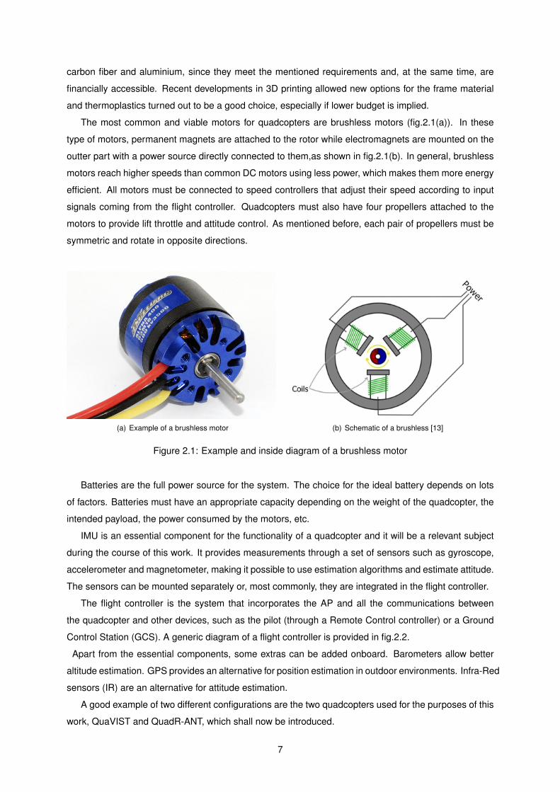
The most common and viable motors for quadcopters are brushless motors (fig.2.1(a)). In these
type of motors, permanent magnets are attached to the rotor while electromagnets are mounted on the
outter part with a power source directly connected to them,as shown in fig.2.1(b). In general, brushless
motors reach higher speeds than common DC motors using less power, which makes them more energy
efficient. All motors must be connected to speed controllers that adjust their speed according to input
signals coming from the flight controller. Quadcopters must also have four propellers attached to the
motors to provide lift throttle and attitude control. As mentioned before, each pair of propellers must be
symmetric and rotate in opposite directions.
(a) Example of a brushless motor (b) Schematic of a brushless [13]
Figure 2.1: Example and inside diagram of a brushless motor
Batteries are the full power source for the system. The choice for the ideal battery depends on lots
of factors. Batteries must have an appropriate capacity depending on the weight of the quadcopter, the
intended payload, the power consumed by the motors, etc.
IMU is an essential component for the functionality of a quadcopter and it will be a relevant subject
during the course of this work. It provides measurements through a set of sensors such as gyroscope,
accelerometer and magnetometer, making it possible to use estimation algorithms and estimate attitude.
The sensors can be mounted separately or, most commonly, they are integrated in the flight controller.
The flight controller is the system that incorporates the AP and all the communications between
the quadcopter and other devices, such as the pilot (through a Remote Control controller) or a Ground
Control Station (GCS). A generic diagram of a flight controller is provided in fig.2.2.
Apart from the essential components, some extras can be added onboard. Barometers allow better
altitude estimation. GPS provides an alternative for position estimation in outdoor environments. Infra-Red
sensors (IR) are an alternative for attitude estimation.
A good example of two different configurations are the two quadcopters used for the purposes of this
work, QuaVIST and QuadR-ANT, which shall now be introduced.
7
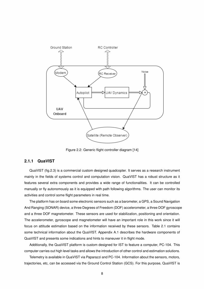
Figure 2.2: Generic flight controller diagram [14]
2.1.1 QuaVIST
QuaVIST (fig.2.3) is a commercial custom designed quadcopter. It serves as a research instrument
mainly in the fields of systems control and computation vision. QuaVIST has a robust structure as it
features several extra components and provides a wide range of functionalities. It can be controlled
manually or fly autonomously as it is equipped with path following algorithms. The user can monitor its
activities and control some flight parameters in real time.
The platform has on board some electronic sensors such as a barometer, a GPS, a Sound Navigation
And Ranging (SONAR) device, a three Degrees of Freedom (DOF) accelerometer, a three DOF gyroscope
and a three DOF magnetometer. These sensors are used for stabilization, positioning and orientation.
The accelerometer, gyroscope and magnetometer will have an important role in this work since it will
focus on attitude estimation based on the information received by these sensors. Table 2.1 contains
some technical information about the QuaVIST. Appendix A.1 describes the hardware components of
QuaVIST and presents some indications and hints to maneuver it in flight mode.
Additionally, the QuaVIST platform is custom designed for IST to feature a computer, PC-104. This
computer carries out high level tasks and allows the introduction of other control and estimation solutions.
Telemetry is available in QuaVIST via Paparazzi and PC-104. Information about the sensors, motors,
trajectories, etc, can be accessed via the Ground Control Station (GCS). For this purpose, QuaVIST is
8

Figure 2.3: QuaVIST platform
Tecnical Info
Carbon Frame
Paparazzi Autopilot
MTOW 5 Kg
Payload Weight 2 Kg
Flight Time Up to 20 minutes
Wind Limit 25 Km/h
Gyroscope 3-axis ADXRS620
Accelerometer 3-axis ADXL335
Magnetometer 3-axis HMC5883L
Table 2.1: Technical specifications of QuaVIST
equipped with a Xbee series datalink, a wireless communication device. Also, the PC-104 can interact
directly with the information received by QuaVIST and send back new information given by the user. A
diagram explaining this flux of information is shown in fig.2.4.
In the case of QuaVIST, the telemetry data is saved into the SD card with a binary format and sent to
the GCS. While the data sent to the GCS can be seen in real time, the same does not happen with the
SD card. To have access to this information, a Matlab program written by Prof. Azinheira, fbin2log.m,
was used. This program turns binary information into readable data by using the Paparazzi flight log.
The log is a file that shows which messages are set to be shown and what type of information they
contain. Some small changes were made in the program in order to have verification of errors, for
9
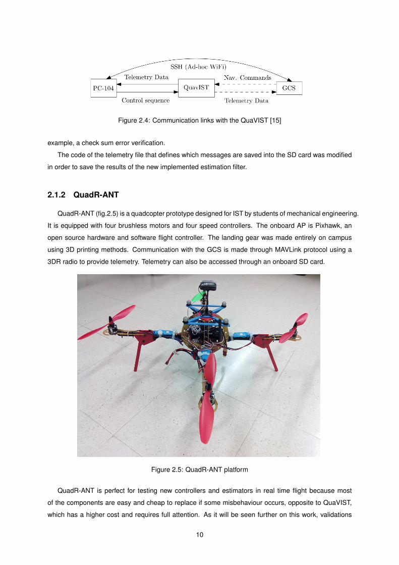
Figure 2.4: Communication links with the QuaVIST [15]
example, a check sum error verification.
The code of the telemetry file that defines which messages are saved into the SD card was modified
in order to save the results of the new implemented estimation filter.
2.1.2 QuadR-ANT
QuadR-ANT (fig.2.5) is a quadcopter prototype designed for IST by students of mechanical engineering.
It is equipped with four brushless motors and four speed controllers. The onboard AP is Pixhawk, an
open source hardware and software flight controller. The landing gear was made entirely on campus
using 3D printing methods. Communication with the GCS is made through MAVLink protocol using a
3DR radio to provide telemetry. Telemetry can also be accessed through an onboard SD card.
Figure 2.5: QuadR-ANT platform
QuadR-ANT is perfect for testing new controllers and estimators in real time flight because most
of the components are easy and cheap to replace if some misbehaviour occurs, opposite to QuaVIST,
which has a higher cost and requires full attention. As it will be seen further on this work, validations
10

during flight were only made using QuadR-ANT because of these reasons.
2.2 Reference Frames
In order to simplify and describe the quadcopter model some assumptions are made [15]:
• The quadcopter is considered to be a rigid body;
• The four propellers are similar;
• The range of the movements is short enough so the Earth rotation and translation can be neglected;
In aviation, a reference system called North East Down (NED) is commonly used. It consists in three
vectors where one represents the position along the northern axis, one along the eastern axis and the
other along the vertical axis. To describe the movement of the quadcopter another frame is necessary,
a body-fixed frame. Let I denote the NED frame (fig.2.6(a)) with center in O, and B the body-fixed
frame with center in Ob (fig.2.6(b)).
(a) NED frame, centered in O (b) Body-fixed frame centered in Ob
(c) Generic NED, IMU and body-fixed frames
Figure 2.6: Reference frames of the quadcopter model [16]
There are cases where the IMU is not located in the center of the body. When dealing with measurements
of the sensors, like it happens with attitude estimation, it is necessary a third frame called the IMU frame.
Let C denote the IMU frame centered in Oc. Figure 2.6(c) shows how the three frames are related
with each other.
11

2.3 Attitude
Attitude is what describes how an object is displaced in space. It represents its orientation, the
imaginary rotation and translation that is necessary to move the object from the current place to a
desired one. Next, basic equations and definitions used to represent attitude are introduced.
2.3.1 Euler Angles
The attitude of the quadcopter is defined by the rotation of the body-fixed frame relatively to the NED
frame. In aeronautics and aviation, Euler angles formulation is commonly used. It states that the rotation
can be described with three angles, each one around each axis:
Ψ =
[φ θ ψ
]T
(2.1)
The Roll , denoted by φ, represents the rotation about the bx axis, the Pitch, denoted by θ, represents
the rotation about the by axis, and, finally the Yaw , denoted by ψ, represents the rotation about the bz
axis, as shown in fig.2.6(b).
The rotation from the inertial frame to the body-fixed frame is done by rotating sequentially each
angle. It is important to notice that the rotations are not commutative and so a certain order must be
held.
The rotation matrix from the inertial frame to the body-fixed frame can be calculated as [17]:
BI RΨ = R(φ)R(θ)R(ψ) (2.2)
where:
R(φ) =
1 0 0
0 cos(φ) sin(φ)
0 − sin(φ) cos(φ)
(2.3)
R(θ) =
cos(θ) 0 − sin(θ)
0 1 0
sin(θ) 0 cos(θ)
(2.4)
R(ψ) =
cos(ψ) sin(ψ) 0
− sin(ψ) cos(ψ) 0
0 0 1
(2.5)
12

By substituing (2.3)-(2.5) in (2.2) we obtain:
BI RΨ =
cos(θ) cos(ψ) cos(θ) sin(ψ) − sin(θ)
sin(φ) sin(θ) cos(ψ)− cos(φ) sin(ψ) sin(φ) sin(θ) sin(ψ) + cos(φ) cos(ψ) sin(φ) cos(θ)
cos(φ) sin(θ) cos(ψ) + sin(φ) sin(ψ) cos(φ) sin(θ) sin(ψ)− sin(φ) cos(ψ) cos(φ) cos(θ)
(2.6)
The order of rotation may also be presented from the body-fixed frame perspective, as shown in
fig.2.7. In this case, the rotation matrix is the transposed/inverted1 of (2.6):
IBRΨ =
cos(θ) cos(ψ) sin(φ) sin(θ) cos(ψ)− cos(φ) sin(ψ) cos(φ) sin(θ) cos(ψ) + sin(φ) sin(ψ)
cos(θ) sin(ψ) sin(φ) sin(θ) sin(ψ) + cos(φ) cos(ψ) cos(φ) sin(θ) sin(ψ)− sin(φ) cos(ψ)
− sin(θ) sin(φ) cos(θ) cos(φ) cos(θ)
(2.7)
Figure 2.7: Rotation from the body-fixed frame to the inertial frame: Yaw-Pitch-Roll [18]
The two rotation perspectives are presented since Pixhawk uses the perspective from the inertial
frame as in (2.6) while Paparazzi uses the perspective from the body-fixed frame, as in (2.7).
Let us address the case when the IMU is not aligned with the body-fixed frame. In such occasions,
in order to compensate this translation, instead of rotating from NED to body-fixed frame directly, first a
rotation from NED to IMU frame is made and then from the latter to the body-fixed frame:
BI RΨ =C
B RTΨ.CI RΨ (2.8)
For the specific case of QuavIST and QuadR-ANT, the IMU is aligned with the quadcopter, meaning
that BCφ = 0, BCθ = 0, BCψ = 0. Using the rotation matrix formulation described in (2.6) and considering
the set of Euler angles to be zero, CBRΨ becomes now the identity matrix:
CBRΨ = I (2.9)
1RΨ is orthogonal and therefore its inverse is equal to its tranpose: R−1 = RT
13

Finally, (2.9) implies:BI RΨ =C
I RΨ (2.10)
Most of the AP’s in the market, like Paparazzi and Pixhawk, are equipped with this algorithm,
allowing the user to set the position parameters of the IMU without additional problems. However,
this implementation was not included within TBF for both AP’s, which means that it is assumed that the
IMU is always aligned with the body-fixed frame. The reason why this algorithm was not implemented
in the AP’s has to do with technical difficulties accessing Paparazzi at the time, and also time issues to
conclude the implementation in Pixhawk. This implementation could be a future improvement to make
the code generic to any quadcopter that uses one of the mentioned AP’s.
When the rotation matrix described in (2.6) is known, the Euler angles can be calculated:
Ψ =
φ
θ
ψ
=
arctan 2(BI R23,
BI R33)
− arcsin(BI R13)
arctan 2(BI R12,BI R11)
(2.11)
where arctan 2 represents the four-quadrant arctangent.
2.3.2 Quaternions
When using the Euler angles approach, a phenomenon called gimbal lock can occur. If a pitch
rotation of θ = (π/2) exists, (2.6) becomes:
BI RΨ =
0 0 −1
sin(φ− ψ) cos(φ− ψ) 0
cos(φ− ψ) − sin(φ− ψ) 0
(2.12)
The rotation matrix has now a singularity and one DOF was lost. The same notation can now represent
two orientations which leads to an ambiguity. To avoid that, one can use a different approach based on
quaternions. Pixhawk uses a quaternion estimator. To integrate the TBF in Pixhawk it is necessary to
convert the Euler angles into quaternions, as explained further in this work.
A quaternion is a vector described as [19]:
q = qi + i qx + j qy + k qz =
[qi qx qy qz
]T, ∈ R4 (2.13)
where i, j, k are unit vectors representing the three Cartesian axes.
A constraint was added comparing with the rotation of three DOF. The quaternion vector q is
normalized for only unitary quaternions, which means that q2i + q2
x + q2y + q2
z = 1.
The quaternions are related with the Euler angles by:
14

q =
[cos(
ψ
2) + k sin(
ψ
2)
] [cos(
θ
2) + j sin(
θ
2)
] [cos(
φ
2) + i sin(
φ
2)
](2.14)
q =
±(cos(φ
2) cos(
θ
2) cos(
ψ
2) + sin(
φ
2) sin(
θ
2) sin(
ψ
2))
±(sin(φ
2) cos(
θ
2) cos(
ψ
2)− cos(
φ
2) sin(
θ
2) sin(
ψ
2))
±(cos(φ
2) sin(
θ
2) cos(
ψ
2) + sin(
φ
2) cos(
θ
2) sin(
ψ
2))
±(cos(φ
2) cos(
θ
2) sin(
ψ
2)− sin(
φ
2) sin(
θ
2) cos(
ψ
2))
(2.15)
The rotation matrix BI Rq can be obtained with the following expression:
BI Rq =
1− 2(q2
y + q2z) 2(qxqy − qiqz) 2(qxqz + qiqy)
2(qxqy + qiqz) 1− 2(q2x + q2
z) 2(qyqz − qiqx)
2(qxqz − qiqy) 2(qyqz + qiqx) 1− 2(q2x + q2
y)
(2.16)
By substituing (2.15) in (2.16) we obtain (2.6).
2.3.3 Attitude Kinematics
Kinematics relates the linear and angular positions of the a body with its velocities. First, let us
introduce some important definitions.
The position of a body, P, is the displacement between Ob and O:
PI =
[X Y Z
]T
(2.17)
Velocity is expressed in the body-fixed frame and is denoted by:
VB =
[U V W
]T
(2.18)
The angular velocity is measured in the body-fixed frame and is described by:
ΩB =
[P Q R
]T
(2.19)
It is possible to relate PI, which defines the position of the body in the inertial frame, and VB, which
defines the velocity in the body-fixed frame, by the following expression:
X
Y
Z
= BI R
T
U
V
W
(2.20)
15

The relation between Ψ and ΩB can be calculated as follows [20]:
ΩB =
P
Q
R
= BI R
T (φ).BI RT (θ).BI R
T (ψ)
0
0
ψ
+ BI R
T (φ).BI RT (θ).
0
θ
0
+ BI R
T (φ).
φ
0
0
(2.21)
which leads to: P
Q
R
=
φ− sin(θ)ψ
cos(φ)θ + cos(θ) sin(φ)ψ
− sin(φ)θ + cos(φ) cos(θ)ψ
(2.22)
Finally, the Euler angles rates can be expressed as:
φ
θ
ψ
=
1 tan(θ) sin(φ) tan(θ) cos(φ)
0 cos(φ) − sin(φ)
0sin(φ)
cos(θ)
cos(φ)
cos(θ)
P
Q
R
(2.23)
Once again one should notice the presence of gimbal lock if θ = ±π2
. To avoid it, the quaternion
form can be used:
qi
qx
qy
qz
=
1
2
0 −P −Q −R
P 0 R −Q
Q −R 0 P
R Q −P 0
qi
qx
qy
qz
(2.24)
For controlling the attitude, in order to achieve stabilization of the quadcopter, it is necessary to
apply a feedback control loop. However, the attitude is not measured directly, which makes estimation
necessary. To accomplish that, measurements provided by sensors are used, as explained in the next
section.
2.4 Inertial Measurement Unit
The Inertial Measurement Unit (IMU) is a device that provides kinematic measurements using inertial
references. It makes use of gyroscopes to measure angular velocities, accelerometers to measure
accelerations and magnetometers to measure magnetic heading. This measures can be later applied
within an estimator to obtain an estimation of the attitude.
16
2.4.1 Gyroscope
Currently, gyroscopes usually are Micro Electro-Mechanical Systems (MEMS), low-cost, small but
still very efficient. The gyroscopes are used to measure the angular velocities of the quadcopter in the
body-fixed frame, ΩB. In this work, an approximation of the gyroscope model is made in order to simplify
the modelling of the system. It is considered that the gyroscope suffers from two kind of disturbances: a
stochastic Gaussian noise and a slowly time-variant non-stochastic bias that can be assumed, most of
the time, as constant [21].
The approximated model that governs the gyroscope can be described as:
ΩB =
[gp gq gr
]T
= ΩB + σω + µω (2.25)
where ΩB ∈ R3 is the measured angular rate, ΩB ∈ R3 is the real angular rate, σω ∈ R3 is the stochastic
Gaussian noise and µω ∈ R3 is the bias.
2.4.2 Accelerometer
Accelerometers are quite useful to measure the acceleration relative to free-fall of a body. This
acceleration is commonly known as g-force and it is different from the acceleration relative to rate of
change of velocity. An accelerometer at rest will measure a positive acceleration of g = 9.81 m/s2 (1G)
upwards while an accelerometer free-falling out of the sky will measure zero acceleration. The physical
principle of an accelerometer is the ordinary concept of a damped mass-spring. When the accelerometer
suffers an acceleration, the mass is displaced to the point where the spring can accelerate the mass at
the same rate. The displacement is measured to calculate the force and, applying Newton’s second law
of motion (~F = m~a), acceleration is obtained. Like the gyroscope, accelerometers are also affected by
the same disturbances described before.
The model of the accelerometer is as follows:
aB = aB −RTΨ.g + σa + µa (2.26)
where aB ∈ R3 is the measured acceleration expressed in the body-fixed frame, aB ∈ R3 is the real
acceleration expressed in the body-fixed frame, g =
[0 0 9.81
]T∈ R3 is the constant gravitational
vector, σa ∈ R3 is the stochastic Gaussian noise and µa ∈ R3 is the bias term.
2.4.3 Magnetometer
Magnetometers are used to measure the local Earth magnetic field. They are also affected by some
disturbances, such as stochastic Gaussian noise, and also local magnetic disturbances such as iron
disturbances, electromagnetic disturbances, etc.
17

The magnetometer model can be characterized as:
n = RTΨ.n + σn + en (2.27)
where n ∈ R3 is the measured magnetic field vector, n ∈ R3 is the real specific local magnetic
field vector, σn ∈ R3 is the stochastic Gaussian noise and en ∈ R3 represents local electromagnetic
interferences affecting the magnetic field.
This work focuses on UAV’s attitude estimation, specially the case of quadcopters and its onboard
implementation to achieve stabilization. In the next section, two AP’s are presented: Paparazzi and
Pixhawk.
2.5 Autopilots
As explained before, AP’s are high level flight controllers that contain control and estimation algorithms,
as well communication protocols that serve as support to the pilot, increasing the level of autonomy of
the aircraft. QuaVIST and QuadR-ANT use different AP’s. They shall now be introduced.
2.5.1 Paparazzi
Paparazzi is a free open-source software and hardware project that provides a range of useful tools
and interfaces for aerial systems2. Its main hardware includes a based board, which incorporates the
IMU sensors, and a GPS receiver. The main board is where the core of the system is located. It is
composed by a set of STM32 series microcontrollers that execute the implemented algorithms. An
example of a based board is illustrated in fig.2.8.
There are two main types of aircrafts that Paparazzi handles, fixed-wing and rotorcraft. The fixed-wing
aircraft is one that does not allow vertical take-off, such as planes or gliders. A rotorcraft allows VTOL,
as in the case of helicopters or quadcopters. This work focuses on the case of a rotorcraft.
Paparazzi is a complex system developed by several people with different backgrounds and methods.
Although there is a developer code and guidelines, it is sometimes very hard to understand its full
functionality. Mainly, there are two ways of making use of Paparazzi: as a user and as a developer.
The user simply adjusts some configuration parameters according to his aircraft platform. A developer
implements new algorithms and methods in the internal core of the system. This work falls under the
developer category since the goal is to modify the attitude estimation algorithm currently being used.
The programming language used in Paparazzi is C.
Because there are two ways of using Paparazzi, the program is divided in two main categories: the
configuration and the airborne structure. The configuration is meant to the common user to change
parameters such as control gains, weight of the platform, direction of the propellers, position of the IMU,
2Paparazzi Wiki, https://wiki.paparazziuav.org/
18

Figure 2.8: Example of an AP based board, Lisa/S [22]
etc. The airborne is a more complex structure that is the core of the program. It contains all the modules,
subsystems, algorithms, algebra methods and firmwares that allow the good performance of Paparazzi.
A functional diagram of the airborne structure is shown in fig.2.9 and it will be presented in the next
subsections. The green areas indicate which subsystems were changed for the purpose of this work.
As one can see in fig.2.9, the airborne architecture consists of the interaction between the AP and
the Fly By Wire (FBW) system. The AP is a group of modules and subsystems designed for auto
control of the aircraft while the FBW is the system that allows the manual control of the aircraft via an
electronic interface by converting the flight controls into electronic signals. It is important to notice that
even when manual mode is set, there is always a commitment between the pilot instructions and the
control algorithms provided by the AP.
Estimation
As explained in the previous chapters, estimation intends to attenuate the noise coming from the
sensors as well to estimate variables that cannot be measured. Paparazzi provides an estimator that
is divided into two subsystems: the Attitude and Heading Reference System (AHRS) and the Inertial
Navigation System (INS).
The AHRS contains a set of algorithms to estimate the attitude, such as the Kalman filter approach
or the CF. These methods use the information provided by the IMU. Paparazzi also provides a method
using the Infra Red (IR) sensors for attitude estimation, by measuring the heat difference between two
sensors on the same axis.
The INS is a subsystem designed for position estimation. It uses GPS information and it is always
connected with the AHRS, due to kinematics that depend on attitude estimation.
19

Figure 2.9: Paparazzi airborne functional diagram [23]
Control
Paparazzi provides a set of PID controllers [24] that run periodically and execute commands for
the servos or for other controllers. The main controllers are the navigation, altitude and stabilization
controllers. The navigation module is loosely based on the work done by D. Biezad [25].
Although this work does not focus on the controlling part, it is important to understand the basic
structure for future developments.
The control loops diagram is illustrated in fig.2.10.
Communications
Communications between Paparazzi agents are basically divided in two fields that interact dynamically:
Datalink and Telemetry.
Datalink is a device consisting of a transmitter, a receiver and a telecommunication circuit that is
governed by a link protocol in order to transmit digital data. In UAV’s it is usually bidirectional, i.e, it
sends control signals and receives telemetry data. A big disadvantage of datalink is that the bandwidth
is limited and signal is often lost, which can cause lost of information and, in the worst case scenario,
20
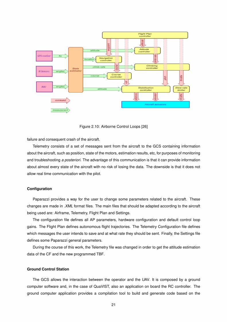
Figure 2.10: Airborne Control Loops [26]
failure and consequent crash of the aircraft.
Telemetry consists of a set of messages sent from the aircraft to the GCS containing information
about the aircraft, such as position, state of the motors, estimation results, etc, for purposes of monitoring
and troubleshooting a posteriori. The advantage of this communication is that it can provide information
about almost every state of the aircraft with no risk of losing the data. The downside is that it does not
allow real time communication with the pilot.
Configuration
Paparazzi provides a way for the user to change some parameters related to the aircraft. These
changes are made in .XML format files. The main files that should be adapted according to the aircraft
being used are: Airframe, Telemetry, Flight Plan and Settings.
The configuration file defines all AP parameters, hardware configuration and default control loop
gains. The Flight Plan defines autonomous flight trajectories. The Telemetry Configuration file defines
which messages the user intends to save and at what rate they should be sent. Finally, the Settings file
defines some Paparazzi general parameters.
During the course of this work, the Telemetry file was changed in order to get the attitude estimation
data of the CF and the new programmed TBF.
Ground Control Station
The GCS allows the interaction between the operator and the UAV. It is composed by a ground
computer software and, in the case of QuaVIST, also an application on board the RC controller. The
ground computer application provides a compilation tool to build and generate code based on the
21

configuration files and the airborne architecture. To load the program into the aircraft, a bootloader
STM32 must be used.
A brief explanation of the configuration and build processes is shown in fig.2.11.
Figure 2.11: Configuration and Build Processes
22

Dependency Files
To have a better practical understanding of what files were modified in the Airborne architecture, the
diagram in fig.2.12 shows, marked in green, the changed files and how they are connected inside the
airborne. The main file, ahrs int cmpl euler.c, is where the Paparazzi CF is located and where the TBF
was implemented.
Figure 2.12: Airborne Dependency Files [27]
In the next section, another AP is introduced, Pixhawk.
2.5.2 Pixhawk
Pixhawk (fig.2.13), much like Paparazzi, is an open-source hardware/software AP that supports
several types of vehicles, such as fixed-wings, helicopters, quadcopters, boats, etc. Its structure is a
bit different from the Paparazzi, providing a more interactive environment between its components.
Its main hardware consists og a 32bit STM32F427 Cortex M4 core processor, a ST Micro L3GD20H
16 bit gyroscope and ST Micro LSM303D 14 bit accelerometer and magnetometer. It has the capacity
to store an SD card in order to save flight logs and also to perform pre-required tasks. The user can
implement commands on the SD card that will execute when pixhawk is turned on.
The software structure of Pixhawk is illutrated in fig.2.14. The grey boxes represent the default
disabled components of Pixhawk. As it can be seen, Pixhawk also provides algorithms for mission
planning and trajectory control. The block represented in green was modified in order to incorporate the
TBF solution.
23

Figure 2.13: Pixhawk AP [28]
Figure 2.14: Pixhawk overview diagram
Estimation
Pixhawk provides two solutions for attitude estimation: an Extended Kalman Filter and a Quaternion-based
Estimator (QBE). The latter is used by default. The controllers onboard Pixhawk receive estimated
variables from these estimators. In order to control not only attitude, but also position and altitude,
estimation of variables such as angular velocities is required. Since the TBF only estimates attitude, it
was necessary to incorporate TBF in the QBE solution to be able to feed the controllers with estimated
variables.
24

Communications
One of the interesting facts about Pixhawk is that their components work as separate modules,
kind of independent applications that communicate with each other when necessary. This allows a
level of flexibility when developing new algorithms and solutions that cannot be achieved in Paparazzi.
Communication between modules is made through asynchronous messages using Micro Object
Request Broker (uORB) protocol. uORB is a middleware solution that allows calls between computers
or topics. A topic is a message that carries out specific information about a system. Pixhawk provides a
wide range of topics containing data about the sensors, the controllers, the IMU, the state of the motors,
etc. Calls are made using handlers, called subscribe and publish. To read information of a topic the
developer must subscribe the topic while to send information to the topic the developer must publish that
information. For the purpose of the TBF implementation, three topics were used: sensors combined,
vehicle attitude and control state. The first topic contains compact data about IMU sensors, that is then
used to estimate attitude. The second topic carries out the information about attitude estimation and that
is where TBF attitude is published along QBE attitude. The last topic contains the estimated variables
that are necessary to feed the controllers.
Communication with GCS is made through MAVLink protocol, a protocol designed as a massive
message library that provides viable communication between small unmanned vehicles and the GCS.
MAVLink reads the topics provided by Pixhawk and sends the information to the GCS. It contains lots
of definitions that allow to send a wide range of information3. The most common GCS for Pixhawk is
qGroundControl, an open source GCS that provides a clean user interface for real time flight management.
The next chapter addresses the attitude estimation problem in detail. The TBF solution is also
introduced.
3Pixhawk MAVLink, https://pixhawk.ethz.ch/mavlink/
25
Chapter 3
Attitude Estimation
For feedback control purposes, the variables one wants to control need to be observable. However,
some of them are not, like the case of the attitude. Attitude cannot be directly measured due to lack of
accurate sensors, and so, it has to be estimated. Estimation also allows reduction of some disturbances,
such as noise and bias from the measurements.
Most of the time is possible to estimate the attitude using a standard IMU of 3-axis accelerometer,
3-axis magnetometer and 3-axis gyroscope with good results. However, some solutions consist on using
more sensors to improve the measurements and accuracy, for example, using vision solutions with on
board cameras.
The Kalman Filter (KF) and the CF are two of the most known and used solutions in the market for
attitude estimation [16]-[29]. The KF is a recursive method that estimates prediction values based on
known control inputs and measurements from the sensors. The CF consists on fusing the information
from the gyroscope and accelerometer, filtering the respective disturbance of each sensor and attributing
them a specific weight. The CF is one of the estimation solutions available in Paparazzi.
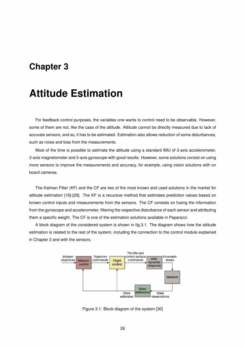
A block diagram of the considered system is shown in fig.3.1. The diagram shows how the attitude
estimation is related to the rest of the system, including the connection to the control module explained
in Chapter 2 and with the sensors.
Figure 3.1: Block diagram of the system [30]
26
3.1 Direct Attitude Estimation
Several estimation methods, including the TBF approach, require a measured rotation matrix, R,
obtained via sensor measurements.
A method to calculate R is to use the Single Value Decomposition (SVD) solution to Wahba’s
problem. This solution consists in minimizing the cost function [31]:
J(R) =1
2
N∑k=1
wk‖ik −Rbk‖2 (3.1)
where ik is the measurement in the reference frame, i.e, the constant gravitational acceleration and the
specific Earth magnetic field vector, bk is the measurement in the body-fixed frame, i.e, the accelerometer
and magnetometer measurements, and wk is an optional set of weights for each observation.
Another method that can be used to obtain R is to compute directly the pitch and roll angles using
the accelerometer measurements [21]. Let a = [ax; ay; az] define the accelerometer measurements in
each axis. Then:
φ = atan2 (−ay,−az) (3.2)
θ = atan2(ax,√a2y + a2
z
)(3.3)
Now, let M = [Mx; My; Mz] define the measurements of the magnetometer in each axis. To obtain
the measured yaw angle, the following equation is used [30]:
ψ = atan2(−My cos φ+ Mz sin φ; Mx cos θ + (My sin φ+ Mz cos φ) sin θ
)(3.4)
The rotation matrix IBR is then obtained by replacing the measured angles in (2.7).
This approach was chosen for the purpose of this work since it is the same method used by Paparazzi.
3.2 Paparazzi Complementary Filter
The main idea behind a CF is to combine the outputs of the gyroscope and accelerometer in
order to obtain good angular estimation results. As described in Chapter 2, both the gyroscopes and
accelerometers suffer from several types of disturbances that have to be filtered somehow.
Accelerometers are very sensitive to vibrations and other non-gravity accelerations in the short term
but it is reliable in the long term. So, the information must go through a Low-Pass Filter to be more
trustworthy.
When it comes to the gyroscope, because of the integration over time, the measurements tend to
drift over time, which means that the data is more reliable on the short term. It is necessary to use a
High-Pass Filter to get good measurements. The function of the CF is to fuse these information in order
27
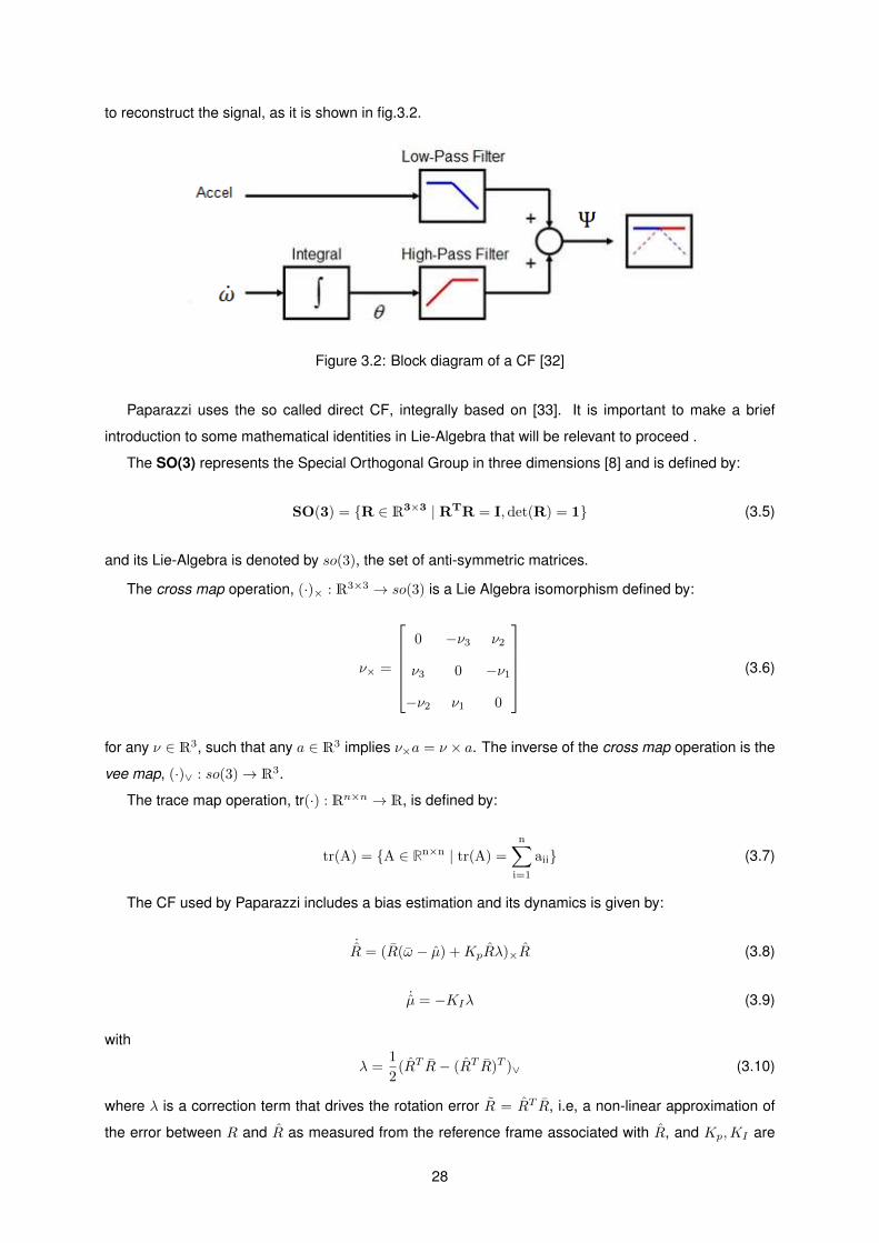
to reconstruct the signal, as it is shown in fig.3.2.
Figure 3.2: Block diagram of a CF [32]
Paparazzi uses the so called direct CF, integrally based on [33]. It is important to make a brief
introduction to some mathematical identities in Lie-Algebra that will be relevant to proceed .
The SO(3) represents the Special Orthogonal Group in three dimensions [8] and is defined by:
SO(3) = R ∈ R3×3 | RTR = I,det(R) = 1 (3.5)
and its Lie-Algebra is denoted by so(3), the set of anti-symmetric matrices.
The cross map operation, (·)× : R3×3 → so(3) is a Lie Algebra isomorphism defined by:
ν× =
0 −ν3 ν2
ν3 0 −ν1
−ν2 ν1 0
(3.6)
for any ν ∈ R3, such that any a ∈ R3 implies ν×a = ν × a. The inverse of the cross map operation is the
vee map, (·)∨ : so(3)→ R3.
The trace map operation, tr(·) : Rn×n → R, is defined by:
tr(A) = A ∈ Rn×n | tr(A) =
n∑i=1
aii (3.7)
The CF used by Paparazzi includes a bias estimation and its dynamics is given by:
˙R = (R(ω − µ) +KpRλ)×R (3.8)
˙µ = −KIλ (3.9)
with
λ =1
2(RT R− (RT R)T )∨ (3.10)
where λ is a correction term that drives the rotation error R = RT R, i.e, a non-linear approximation of
the error between R and R as measured from the reference frame associated with R, and Kp,KI are
28
positive gains.
3.3 Trace-based Filter
The core of this approach consists in considering an attitude error function Υ : SO(3)×SO(3)→ R,
an attitude error vector er ∈ R3 and an angular velocity error vector eω ∈ R3:
Υ(R, R) =1
2tr(
D(I− RTR))
(3.11)
eR =1
2
[DRTR− RTRD
]∨
(3.12)
eω = ω − RTRω (3.13)
where Υ(R, R) is a locally positive-definite about R = R and D ∈ R3×3 is a positive definite diagonal
weighting matrix.
3.3.1 Continuous Time Formulation
For a known measured rotation matrix R and known angular velocity measurements ω (gyroscope
measurements), and based on (3.11)-(3.13), the estimator dynamics is:
eω = −∆eω −d
2
[DRT R− RT RD
]∨
(3.14)
R = R [ω]× (3.15)
for
ω = eω + RT Rω (3.16)
where ∆ is a positive definite diagonal weighting matrix and d ∈ R+ is a positive scalar parameter.
The design parameters have a specific effect on the estimator. The scalar parameter d determines
the influence of the vectorial measurements in eR. Matrix ∆ determines the impact of the previous
angular velocity estimation into the present one. Weighting matrix D sets the importance of the attitude
correction provided by R on roll, pitch and yaw individually.
3.3.2 Discrete Time Formulation
For a sampling time ts, the discrete formulation (3.14)-(3.15) can be rewritten as:
eω,k+1 = eω,k − ts∆eω,k − tsdeR (3.17)
29
Rk+1 = Rk expts[ω]× (3.18)
where the angular velocity estimation, ωk, is given by:
ωk = eω,k + RTk Rkωk (3.19)
and
expts[ω]× = I + [ω]× sin (ts) + [ω]2× [1− cos (ts)] (3.20)
3.3.3 Gyroscope Bias Estimation
As explained previously in Chapter 2, low cost MEMS gyroscopes usually have small disturbances,
one of them being a slowly time varying bias, µω, described by (2.25). It is possible to estimate the
gyroscope bias in order to reduce its impact on the attitude results.
The used bias formulation is the following:
ω = ω + α− µ, ˙µ = −kµα (3.21)
where α is a correction term based on the vectorial measurements and 0 < kµ < 1.
Rearranging (3.21), we obtain:
α = ω − ω + µ (3.22)
One should notice that the TBF has a rotation between the frames of ω and ω, so the correction term
α can be redefined as:
α = ω − RT Rω + RT Rµ (3.23)
which can also be represented by
α = eω + RT Rµ ∴ ˙µ = −kµ(eω + RT Rµ
)(3.24)
Algorithm 3.1 describes the implementation of the TBF without bias estimation, i.e, the standard
formulation. Algorithm 3.2 presents the implementation of TBF with bias estimation described in (3.21).
The next chapter addresses the implementation of such algorithms in Paparazzi and Pixhawk and
the results are discussed.
30

Algorithm 3.1 TBF discrete algorithm without bias estimation1: Input: gyro, accel, mag . 3x1 vectors containing sensors information2: Initialize:3: d, ts4: D = diag(D11, D22, D33)5: ∆ = diag(∆11,∆22,∆33)6: R0 = I(3)7: eω,0 = zeros(3, 1)
8: ΨTBF=empty matrix9:
10: for int k=1 to k=length(gyro) do11: φk = atan2(−accelk,2;−accelk,3)
12: θk = atan2(accelk,1;√accel2k,2 + accel2k,3)
13: mek = −magk,2 cos φk +magk,3 sin ψk14: mnk = magk,1 cos φk +magk,2 sin φk sin θk +magk,3 cos φk sin θk15: ψk = atan2(mek;mnk)16:
17: Rφ,k =
1 0 0
0 cos(−φk) sin(−φk)
0 − sin(−φk) cos(−φk)
18: Rθ,k =
cos(−θk) 0 − sin(−θk)
0 1 0
sin(−θk) 0 cos(−θk)
19: Rψ,k =
cos(−ψk) sin(−ψk) 0
− sin(−ψk) cos(−ψk) 0
0 0 1
20: Rk = Rψ,kRθ,kRφ,k21:22: edotk = d
2
[DRTk Rk−1 − RTk−1RkD
]23:24: e∨k = [−edotk,23; edotk,13;−edotk,12] . 3x1 vector25:26: eω,k = eω,k−1 − ts(∆eω,k−1 + e∨k)27:28: ωk = eω,k + RTk−1Rk.gyrok29:
30: ω×,k =
0 −ωk,3 ωk,2
ωk,3 0 −ωk,1−ωk,2 ωk,1 0
31:32: MExpk = I + ω×,k sin ts + ω2
×,k(1− cos ts)
33: Rk = Rk−1MExpk . Matrix exponential of tω×,k34:35: φk = atan2(Rk,23; Rk,33)
36: θk = − arcsin(Rk,13)
37: ψk = atan2(Rk,12; Rk,11)38:39: Ψk =
[φk θk ψk
]40: ΨTBF =
[ΨTBF ; Ψk
]. Concatenates current euler angles in a global matrix of size kx3
41: end for
31

Algorithm 3.2 TBF discrete algorithm with bias estimation1: Input: gyro, accel, mag . 3x1 vectors containing sensors information2: Initialize:3: d, ts, kµ4: D = diag(D11, D22, D33)5: ∆ = diag(∆11,∆22,∆33)6: R0 = I(3)7: eω,0 = zeros(3, 1)
8: ΨTBF=empty matrix9: µ0 = zeros(3, 1)
10:11: for int k=1 to k=length(gyro) do12: φk = atan2(−accelk,2;−accelk,3)
13: θk = atan2(accelk,1;√accel2k,2 + accel2k,3)
14: mek = −magk,2 cos φk +magk,3 sin ψk15: mnk = magk,1 cos φk +magk,2 sin φk sin θk +magk,3 cos φk sin θk16: ψk = atan2(mek;mnk)17:
18: Rφ,k =
1 0 0
0 cos(−φk) sin(−φk)
0 − sin(−φk) cos(−φk)
19: Rθ,k =
cos(−θk) 0 − sin(−θk)
0 1 0
sin(−θk) 0 cos(−θk)
20: Rψ,k =
cos(−ψk) sin(−ψk) 0
− sin(−ψk) cos(−ψk) 0
0 0 1
21: Rk = Rψ,kRθ,kRφ,k22:23: edotk = d
2
[DRTk Rk−1 − RTk−1RkD
]24:25: e∨k = [−edotk,23; edotk,13;−edotk,12] . 3x1 vector26:27: eω,k = eω,k−1 − ts(∆eω,k−1 + e∨k)28:29: ωk = eω,k + RTk−1Rk(gyrok − µk−1)30:
31: ω×,k =
0 −ωk,3 ωk,2
ωk,3 0 −ωk,1−ωk,2 ωk,1 0
32:33: MExpk = I + ω×,k sin ts + ω2
×,k(1− cos ts)
34: Rk = Rk−1MExpk . Matrix exponential of tω×,k35:36: µk = µk−1 −Kµ.ts(ωk − RTk Rk.gyrok + RTk Rkµk−1) . Updates bias for the next iteration37: φk = atan2(Rk,23; Rk,33)
38: θk = − arcsin(Rk,13)
39: ψk = atan2(Rk,12; Rk,11)40:41: Ψk =
[φk θk ψk
]42: ΨTBF =
[ΨTBF ; Ψk
]. Concatenates current euler angles in a global matrix of size kx3
43: end for
32

Chapter 4
Implementations and Results
The implementation of the TBF was made in two AP’s: Paparazzi and Pixhawk.
For the case of Paparazzi, first, some data from QuaVIST sensors were taken for a known trajectory
in order to reconstruct the TBF in Matlab, with and without bias estimation. Then, after implementation,
a comparison was made between the Matlab results, the implemented TBF on Paparazzi and the CF on
Paparazzi, using the true ground attitude values provided by a motion capture system mounted in IST,
called Arena.
For the case of Pixhawk, results from the TBF implementation were taken during a real-time flight
and compared against data provided by Arena. A validation was not made on Matlab for this case
due to technical difficulties in obtaining valid data from the Pixhawk IMU. Also, a comparison with the
quaternion estimator used by Pixhawk could not be made because in real-time flight it was only possible
to get data from the estimator being used.
In the next sections, these results and validation are presented and discussed to obtain the proper
conclusions.
4.1 Paparazzi Implementation
For the purpose of this validation, data from QuaVIST sensors, as well attitude estimation from the CF
and the implemented TBF, were saved on a SD card. A simple trajectory was described with QuaVIST
with the motors turned off and it consists on small roll and pitch rotations in both directions and yaw
rotations of about 90 , also in both directions. The TBF parameters were adjusted manually until good
performance was achieved. Paparazzi IMU runs at 100Hz while the complete estimator runs at 512Hz.
To achieve good performance, the complete integration of the TBF on Paparazzi estimator was set to run
at 512Hz. The telemetry message was set for 20Hz. Arena provides data at 179Hz. At the time of this
implementation, kµ was set to zero because no data from Arena was available and it would be impossible
to validate the impact of the bias estimation without the true ground values. Due to technical difficulties
(failure in compiling Paparazzi code with recent versions), a more recent implementation failed. So, for
the purposes of validation of bias estimation, an impact analysis was made on Matlab for different values
33

of kµ. Table 4.1 summarizes the values of the TBF used in the implementations.
Values of the TBF parametersMatlab implementation Paparazzi implementation
Frequency [Hz] 100 512d 10 4D diag(25, 25, 25) diag(25, 25, 25)
∆ diag(45, 45, 45) diag(45, 45, 45)
kµ 0.1 0
Table 4.1: Values of the TBF parameters for the Matlab and Paparazzi implementations
4.1.1 Paparazzi Results
The implementation of the TBF on Matlab derives from the data provided by the IMU of QuaVIST:
the gyroscope, accelerometer and magnetometer. Fig.4.1 illustrates the data from the sensors for the
previously mentioned trajectory. In order to compare data with different frequencies, a resample was
made using methods of interpolation and decimation.
From these measurements it was possible to provide an estimation for attitude in Matlab with and
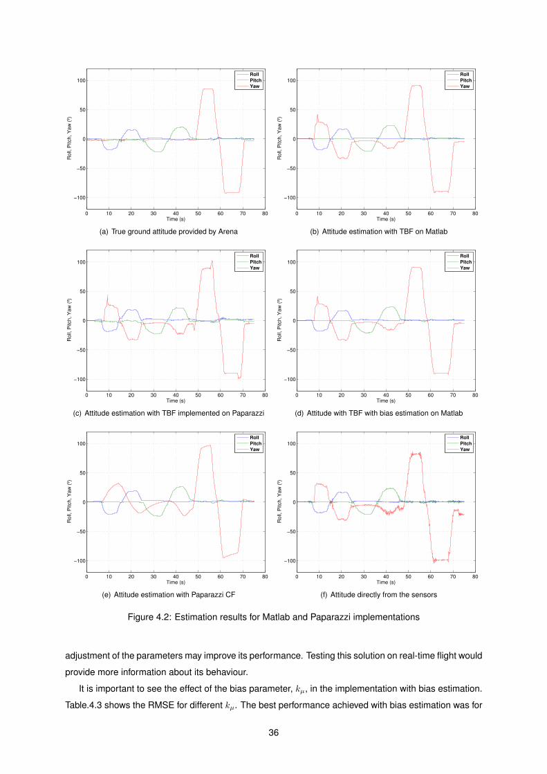
without bias estimation and compare them against the CF and Arena. Fig.4.2 shows each set of Euler
angles for each implementation and fig.4.3 presents a comparison between each implementation for roll,
pitch and yaw rotations.
Some quick conclusions can be drawn from fig.4.2. It is visible that all implementations follow the
dynamics of the attitude, at least for roll and pitch rotations, setting fig.4.2(a) as the reference. For yaw
rotation, there are a few notes to be explained. First of all, the initial offset of the magnetometer seen in
fig.4.1(c) was removed in order to have a cleaner visual plot of yaw estimation. This offset has to do with
how many degrees the quadcopter is displaced from the north at the initial time and does not interfere
with the validation of the attitude estimation.
Another difference one can see for the yaw rotation, when compared with fig.4.2(a), is that there are
rotations in both positive and negative directions in the interval of about [t = 10, 50]. This is most likely
due to magnetometer miscalibration. The magnetometer follows the roll and pitch rotations which is not
supposed to happen. When looking at interval n = [1000, end] one can see the correct dynamics of the
yaw.
From fig.4.3 it is possible to see the performance of each implementation individually for each axis.
The TBF on Matlab shows a very good performance, following the Arena reference. Implementation on
Paparazzi shows good dynamics but with more noise. This is most likely due to the internal system of
paparazzi, for example, the frequency at which the estimator runs it is different from the IMU.
It is also important to note that the TBF follows the measures from the sensors. Comparing the TBF
and the CF with Arena for yaw rotations (fig.4.3(c)), one can see that the rotations in the interval of
34

0 10 20 30 40 50 60 70 80−80
−60
−40
−20
0
20
40
60
Time (s)
Angula
r velo
city [º/
s]
gp
gq
gr
(a) Measured angular velocity by the gyroscope
0 10 20 30 40 50 60 70 80−12
−10
−8
−6
−4
−2
0
2
4
Time (s)
Accele
ration [m
/s2]
ax
ay
az
(b) Measured acceleration by the accelerometer
0 10 20 30 40 50 60 70 80−1
−0.5
0
0.5
1
1.5
2
Time (s)
Magnetic fie
ld [norm
aliz
ed]
mx
my
mz
(c) Measured magnetic field by the magnetometer
Figure 4.1: Data from QuaVIST sensors
n = [200; 900] come from the sensors and that the estimators tend to follow that information.
In order to obtain a detailed analyse of the performance of each estimator, a calculation of the
Root-Mean-Square Error (RMSE) was made:
RMSE =
√∑ni=1(Ψi − Ψi)2
n(4.1)
where Ψi represents the true ground values of attitude, in this case provided by Arena, Ψi represents
the estimated values of each solution and n in the number of samples. Table.4.2 resumes the RMSE of
each implementation.
It is possible to observe that, from all the presented solutions, the TBF on Matlab is the one with the
best performance, achieving a smaller error when compared to the CF.
The implementation of the TBF on Paparazzi presents good results. However, attitude worsens when
compared to the implementation on Matlab. Also, this solution appears to contain more noise. A better
35
0 10 20 30 40 50 60 70 80
−100
−50
0
50
100
Time (s)
Ro
ll, P
itch
, Y
aw
(º)
Roll
Pitch
Yaw
(a) True ground attitude provided by Arena
0 10 20 30 40 50 60 70 80
−100
−50
0
50
100
Time (s)
Ro
ll, P
itch
, Y
aw
(º)
Roll
Pitch
Yaw
(b) Attitude estimation with TBF on Matlab
0 10 20 30 40 50 60 70 80
−100
−50
0
50
100
Time (s)
Ro
ll, P
itch
, Y
aw
(º)
Roll
Pitch
Yaw
(c) Attitude estimation with TBF implemented on Paparazzi
0 10 20 30 40 50 60 70 80
−100
−50
0
50
100
Time (s)
Ro
ll, P
itch
, Y
aw
(º)
Roll
Pitch
Yaw
(d) Attitude with TBF with bias estimation on Matlab
0 10 20 30 40 50 60 70 80
−100
−50
0
50
100
Time (s)
Ro
ll, P
itch
, Y
aw
(º)
Roll
Pitch
Yaw
(e) Attitude estimation with Paparazzi CF
0 10 20 30 40 50 60 70 80
−100
−50
0
50
100
Time (s)
Ro
ll, P
itch
, Y
aw
(º)
Roll
Pitch
Yaw
(f) Attitude directly from the sensors
Figure 4.2: Estimation results for Matlab and Paparazzi implementations
adjustment of the parameters may improve its performance. Testing this solution on real-time flight would
provide more information about its behaviour.
It is important to see the effect of the bias parameter, kµ, in the implementation with bias estimation.
Table.4.3 shows the RMSE for different kµ. The best performance achieved with bias estimation was for
36

0 10 20 30 40 50 60 70 80−30
−20
−10
0
10
20
30
Time (s)
Roll
(º)
Arena
TBF on Matlab
TBF on Paparazzi
TBF w/ Bias on Matlab
CF Paparazzi
Sensors Attitude
(a) Roll
0 10 20 30 40 50 60 70 80−30
−20
−10
0
10
20
30
Time (s)
Pitch (
º)
Arena
TBF on Matlab
TBF on Paparazzi
TBF w/ Bias on Matlab
CF Paparazzi
Sensors Attitude
(b) Pitch
0 10 20 30 40 50 60 70 80−150
−100
−50
0
50
100
150
Time (s)
Ya
w (
º)
Arena
TBF on Matlab
TBF on Paparazzi
TBF w/ Bias on Matlab
CF Paparazzi
Sensors Attitude
(c) Yaw
Figure 4.3: Roll, Pitch and Yaw results for Matlab and Paparazzi implementations
kµ = 0.1. The estimated attitude tends to get worse with the increase of kµ, except for the case of φ,
that improves slightly.
37

RMSE[ ] φ θ ψ
TBF on Matlab 1.218 1.822 15.221TBF on Paparazzi 2.099 2.433 13.838TBF w/ bias on Matlab 1.212 1.854 15.303CF 2.034 2.458 15.966
Table 4.2: RMSE for Matlab and Paparazzi implementations
RMSE[ ] φ θ ψ
kµ = 0.1 1.212 1.854 15.303kµ = 0.2 1.210 1.883 15.433kµ = 0.5 1.203 1.955 15.917kµ = 0.8 1.194 2.007 16.394kµ = 1 1.189 2.034 16.712
Table 4.3: RMSE for TBF on Matlab, for different bias parameter, kµ
In the next section, an analysis of attitude estimation is presented in real-time flight with QuadR-ANT,
on Pixhawk.
4.2 Pixhawk Implementation
In order to test the performance of the TBF in real scenarios, a flight with random trajectories was
conducted using QuadR-ANT. The attitude data was taken in real-time and saved in a log file. True
ground values were also taken from Arena to conclude about TBF performance. However, reliable data
from the sensors could not be obtained in order to implement the TBF solution on Matlab and compare
it with the default quaternion estimator of Pixhawk.
Table.4.4 resumes the values of the parameters implemented on Pixhawk for the TBF solution. The
whole Pixhawk system runs at 250Hz while Arena remains at 179Hz.
Values of the TBF parametersPixhawk implementation
Frequency [Hz] 250d 4D diag(25, 25, 25)
∆ diag(45, 45, 45)
kµ 0.1
Table 4.4: Values of the TBF parameters for the Pixhawk implementation
38
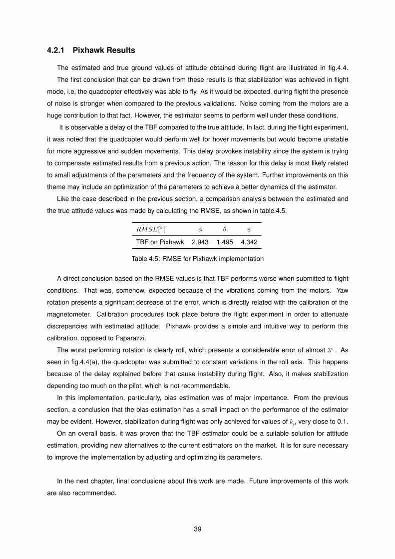
4.2.1 Pixhawk Results
The estimated and true ground values of attitude obtained during flight are illustrated in fig.4.4.
The first conclusion that can be drawn from these results is that stabilization was achieved in flight
mode, i.e, the quadcopter effectively was able to fly. As it would be expected, during flight the presence
of noise is stronger when compared to the previous validations. Noise coming from the motors are a
huge contribution to that fact. However, the estimator seems to perform well under these conditions.
It is observable a delay of the TBF compared to the true attitude. In fact, during the flight experiment,
it was noted that the quadcopter would perform well for hover movements but would become unstable
for more aggressive and sudden movements. This delay provokes instability since the system is trying
to compensate estimated results from a previous action. The reason for this delay is most likely related
to small adjustments of the parameters and the frequency of the system. Further improvements on this
theme may include an optimization of the parameters to achieve a better dynamics of the estimator.
Like the case described in the previous section, a comparison analysis between the estimated and
the true attitude values was made by calculating the RMSE, as shown in table.4.5.
RMSE[ ] φ θ ψ
TBF on Pixhawk 2.943 1.495 4.342
Table 4.5: RMSE for Pixhawk implementation
A direct conclusion based on the RMSE values is that TBF performs worse when submitted to flight
conditions. That was, somehow, expected because of the vibrations coming from the motors. Yaw
rotation presents a significant decrease of the error, which is directly related with the calibration of the
magnetometer. Calibration procedures took place before the flight experiment in order to attenuate
discrepancies with estimated attitude. Pixhawk provides a simple and intuitive way to perform this
calibration, opposed to Paparazzi.
The worst performing rotation is clearly roll, which presents a considerable error of almost 3 . As
seen in fig.4.4(a), the quadcopter was submitted to constant variations in the roll axis. This happens
because of the delay explained before that cause instability during flight. Also, it makes stabilization
depending too much on the pilot, which is not recommendable.
In this implementation, particularly, bias estimation was of major importance. From the previous
section, a conclusion that the bias estimation has a small impact on the performance of the estimator
may be evident. However, stabilization during flight was only achieved for values of kµ very close to 0.1.
On an overall basis, it was proven that the TBF estimator could be a suitable solution for attitude
estimation, providing new alternatives to the current estimators on the market. It is for sure necessary
to improve the implementation by adjusting and optimizing its parameters.
In the next chapter, final conclusions about this work are made. Future improvements of this work
are also recommended.
39

0 10 20 30 40 50 60 70 80−8
−6
−4
−2
0
2
4
6
8
Time (s)
Roll
(º)
Arena
TBF on Pixhawk
(a) Roll
0 10 20 30 40 50 60 70 80−8
−6
−4
−2
0
2
4
6
8
Time (s)
Pitch (
º)
Arena
TBF on Pixhawk
(b) Pitch
0 10 20 30 40 50 60 70 80−8
−6
−4
−2
0
2
4
6
8
Time (s)
Ya
w (
º)
Arena
TBF on Pixhawk
(c) Yaw
Figure 4.4: Roll, Pitch and Yaw results for Pixhawk implementation
40
Chapter 5
Conclusions
During the course of this work some results were reached and some final conclusion can be draw. A
clearer explanation about the structure of Paparazzi and Pixhawk was provided, which may help future
developers understanding its concept for future improvements.
The implementations of the TBF in both studied AP’s revealed good overall performances. However,
further improvements should be made in order to get more accurate results. Improvements should
focus on the optimization of parameters. Results of the implementation on Paparazzi show very good
performances for roll and pitch rotations, yielding slightly better results than the CF. For yaw rotation,
poor results were obtained considering magnetometer miscaliberation. It was demonstrated that estimation
of bias has a positive impact for small values of kµ and tends to worsen when increased. The bias
estimation was crucial for the Pixhawk implementation, since stability conditions for the flight were only
achieved when bias estimation was present, with kµ = 0.1.
A well succeeded flight experiment was achieved for the Pixhawk implementation, which is, by itself,
a good indicator. In this case, the TBF estimator performs worse and becomes unstable for sudden and
aggressive movements. Although reasonable results were obtained and flight was possible, this does
not discard future improvements, specially for purposes of computational vision and aerial mapping,
where stabilization is of maximum importance.
Another interesting improvement that could be made in the future include combining the TBF solution
with new control solutions. Substituting the PID controllers being used by both AP’s by LQR based
solutions might provide new perspectives about attitude control and estimation. In the case of Paparazzi,
this improvement might help with the high level control tasks taking place in PC-104, giving the user
more autonomy and flexibility. Testing and analysing the performance of such solution is an interesting
development to be made.
Over the course of this work, Pixhawk revealed to be a simpler and more user friendly tool, not only
for the user but for developers. Thus, installing Pixhawk on QuaVIST may prove to be a good choice.
Some of the work done here may help this transition.
41

Bibliography
[1] J. McHale. Unmanned Aircraft Are Coming to a Sky Near You. Military Embedded Systems, 8(5):
8, July/August 2012.
[2] S. Waharte and N. Trigoni. Supporting Search and Rescue Operations with UAVs. In Emerging
Security Technologies (EST), 2010 International Conference on, pages 142–147. IEEE, 2010.
[3] D. Rondao. Modeling and Simulation of the ECOSat-III Attitude Determination and Control System.
Master Thesis, Instituto Superior Tecnico, Universidade de Lisboa, April 2016.
[4] L. Harris. Police drones take off: Secret weapons in the fight against crime and terror attacks.
http://www.dailytelegraph.com.au/. [Online; last time accessed: 27-April-2016].
[5] M. Taj. Archaeologists use drones in peru to map and protect sites. http://www.thestar.com.my/.
[Online; last time accessed: 24-April-2016].
[6] W. K. Roustan. Live from pompano beach: Drones tested to prevent ocean drownings. http:
//www.sun-sentinel.com/. [Online; last time accessed: 25-April-2016].
[7] R. Verrier. Drones are providing film and tv viewers a new perspective on the action. http://www.
latimes.com/. [Online; last time accessed: 25-April-2016].
[8] A. Moutinho, M. Figueiroa, and J. R. Azinheira. Attitude Estimation in SO(3): A Comparative UAV
Case Study. Journal of Intelligent & Robotic Systems, 80(3-4):375–384, 2015.
[9] S. B. Anderson. Historical Overview of V/STOL Aircraft Technology. NASA Technical Memorandum
81280, January 1997.
[10] P. Theodorakopoulos. On Autonomous Target Tracking for UAVs. PhD thesis, Universite de
Toulouse, 2009.
[11] Quadcopter ArenA. URL http://quadcopterarena.com/the-history-of-drones-and-quadcopters/.
[Online; last time accessed: 25-August-2015].
[12] M. Figueiroa. Nonlinear Attitude Estimation in SO(3): Application to a Quadrotor UAV. Master
Thesis, Instituto Superior Tecnico, Universidade de Lisboa, May 2014.
[13] Black Tie Aerial. URL http://blacktieaerial.com/selecting-motors/. [Online; last time
accessed: 29-April-2016].
42
[14] H. Chao, Y. Cao, and Y. Chen. International Journal of Control, Automation and Systems, 8(1):
36–44, 2010.
[15] B. Oliveira. Quadrotor Stabilization using Visual Servoing. Master Thesis, Instituto Superior
Tecnico, Universidade Tecnica de Lisboa, 2013.
[16] B. Henriques. Estimation and Control of a Quadrotor Attitude. Master Thesis, Instituto Superior
Tecnico, Universidade Tecnica de Lisboa, June 2011.
[17] B. L. Stevens and F. L. Lewis. Aircraft control and simulation, john wiley & sons. Inc., New York,
1992.
[18] D.L Engineering. URL http://dle-tech.info/tag/pitch/. [Online; last time accessed:
6-May-2016].
[19] L. Vicci. Quaternions and rotations in 3-space: The algebra and its geometric interpretation.
TR01–014, pages 1–11, 2001.
[20] W. E. Wiesel. Spaceflight Dynamics. Mc-Graw Hill, 2nd edition, 1996.
[21] M. Euston, P. Coote, R. Mahony, J. Kim, and T. Hamel. A Complementary Filter for Attitude
Estimation of a Fixed-Wing UAV. In Intelligent Robots and Systems, 2008. IROS 2008. IEEE/RSJ
International Conference, pages 340–345, Nice, September 2008.
[22] 1BitSquared. URL http://1bitsquared.com/products/lisa-s. [Online; last time accessed:
9-May-2016].
[23] PaparazziWiki. URL http://wiki.paparazziuav.org/wiki/DevGuide/DesignOverview. [Online;
last time accessed: 01-July-2016].
[24] M. A. Botto. Controlo de Sistemas. AEIST, 1st edition, Feb. 2009.
[25] D. J. Biezad. Integrated Navigation and Guidance Systems. AIAA, January 1999.
[26] P. Brisset, A. Drouin, M. Gorraz, P.-S. Huard, and J. Tyler. The Paparazzi Solution. In MAV 2006,
2nd US-European Competition and Workshop on Micro Air Vehicles, 2006.
[27] DocsPaparazzi. URL http://docs.paparazziuav.org/v4.2/ahrs__int__cmpl__euler_8c.html.
[Online; last time accessed: 22-December-2015].
[28] Pixhawk. URL https://pixhawk.org/choice. [Online; last time accessed: 11-May-2016].
[29] P. Batista, C. Silvestre, and P. Oliveira. Sensor-Based Complementary Globally Asymptotically
Stable Filters for Attitude Estimation: Analysis, Design, and Performance Evaluation. Automatic
Control, IEEE Transactions on, 57(8):2095–2100, February 2012.
[30] J. D. Barton. Fundamentals of Small Unmanned Aircraft Flight. Johns Hopkins APL Technical
Digest, 31(2):132–149, 2012.
43

[31] F. L. Markley. Attitude determination using vector observations and the singular value
decomposition. The Journal of the Astronautical Sciences, 36(3):245–258, 1988.
[32] Instructables. URL http://www.instructables.com/id/PCB-Quadrotor-Brushless/step15/
IMU-Part-2-Complementary-Filter/. [Online; last time accessed: 01-July-2016].
[33] R. Mahony, T. Hamel, and J.-M. Pflimlin. Nonlinear Complementary Filters on the Special
Orthogonal Group. Automatic Control, IEEE Transactions on, 53(5):1203–1218, June 2008.
44

Appendix A
QuavIST Schematics
A.1 Scheme of QuavIST components
Figure A.1: Scheme for QuavIST components
A.1

Figure A.2: Schematics Legend
A.2

Introduction
This document is meant to help new users understand some of QuavIST features when
we want to fly it. All the hints and advices come from notes taken at a flight lesson at
UAVision.
1. Radio Controller
QuavIST is equipped with a RC that allows the user to control the drone, including
the throttle, speed, roll, pitch and yaw. It also provides real time information about
the drone (batteries charge, telemetry, position, ect). It’s important to have a good
understanding of the controller and what is each button function.
Buttons subtitles:
1. Return to launch (home)
2. -
3. Turn on RC
4. Turn on IPad (screen)
5. Antenna
6. Mode Auto (mission)
7. Throttle/Velocity Stick (Vertical) and Yaw Stick (horizontal).
8. Assisted Mode
9. Assisted Mode
10. Attitude control stick (horizontal) and Pitch stick (vertical)
1
2 3 4
6
5
7
9
8
10
11
12
11. -
12. Start engines
2. Modes
The drone can be controlled in assisted mode (useful for missions) and manual
mode (complete freedom in control).
2.1 Assisted mode
When in assisted mode, if there are no satellites available (which means no GPS), a
message ‘assisted fail safe’ will appear on the RC screen. When enough satellites
are found (minimum 6 satellites), the chosen mode is RC climb.
In assisted mode the user controls the speed instead of the throttle.
Stick 7 down Velocity 0
Stick 7 middle Velocity 50%
Stick 7 up Velocity 100%
2.2 Manual mode
In manual mode, the user controls the throttle.
Stick 7 down Throttle 0
Stick 7 middle Throttle 50%
Stick 7 up Throttle 100%
In both modes, for QuavIST, the front of the drone is the front of the pilot.
3. Flight Procedures
Before flying with a powerful drone such as QuavIST, one should practice enough
with small quadcopters. It is highly recommended to try controlling those small
quadcopters in a small space (around ) to guarantee a good level piloting
skills.
The procedures that must be followed are:
1. Turn on RC – green lights will be turned on
2. Turn on IPad – when or if asked, the password is ‘idmec’.
3. Turn on the batteries – The batteries should be placed in the small container
right below the paparazzi platform. Special cares should be taken when
connecting them. Before connecting battery nº1, the user must be sure that
terminals of battery nº2 are not touching anything, especially metal platforms,
to avoid short-circuit. After connecting battery nº1, connect battery nº2.

4. Turn on the engines – To do it, the user must put the Throttle Stick (#7)
completely down and press button 12 at the same time. Engines will turn on
one at a time.
5. Test attitude control in the ground – Before taking off, it’s important to see if
the commands are responding. One simple test that should be made is to test
the pitch (forward and backward) and the roll (left and right), always with
minimum throttle (Stick completely down)
6. Take off – If you are flying in ‘manual’ mode with fully charged batteries, you
should release the throttle stick. If batteries are used and not fully charged, put
the stick to maximum (completely up). In assisted mode, if there are enough
satellites available, the chosen mode should be RC climb. In this case just push
the throttle stick all the way up to its maximum.
One way to check if the batteries are fully charged is to release the throttle
stick. If the drone continues to climb it means that the batteries still have
enough power.
7. Landing – To land the drone some cares must be taken. The descent must be
made slowly and not in a vertical direction but rather in a diagonal direction
until about 10 cm from the floor (that prevents the drone of losing its lift and
fall). After stabilizing the drone, the user must turn off the engines (throttle
stick down) until it lands and press button 12 while maintaining the throttle
stick down.