implementation of a dynamic mooring solver (moody) into a

Deliverable D4.6

ISSN 1901-726X DCE Technical Report No. XXX

Implementation of a dynamic

mooring solver (MOODY) into a wave to wire model of a simple

WEC

Francesco Ferri Johannes Palm

DRAFT

Scientific Publications at the Department of Civil Engineering Technical Reports are published for timely dissemination of research results and scientific work carried out at the Department of Civil Engineering (DCE) at Aalborg University. This medium allows publication of more detailed explanations and results than typically allowed in scientific journals. Technical Memoranda are produced to enable the preliminary dissemination of scientific work by the personnel of the DCE where such release is deemed to be appropriate. Documents of this kind may be incomplete or temporary versions of papers—or part of continuing work. This should be kept in mind when references are given to publications of this kind. Contract Reports are produced to report scientific work carried out under contract. Publications of this kind contain confidential matter and are reserved for the sponsors and the DCE. Therefore, Contract Reports are generally not available for public circulation. Lecture Notes contain material produced by the lecturers at the DCE for educational purposes. This may be scientific notes, lecture books, example problems or manuals for laboratory work, or computer programs developed at the DCE. Theses are monograms or collections of papers published to report the scientific work carried out at the DCE to obtain a degree as either PhD or Doctor of Technology. The thesis is publicly available after the defence of the degree. Latest News is published to enable rapid communication of information about scientific work carried out at the DCE. This includes the status of research projects, developments in the laboratories, information about collaborative work and recent research results.

Published YYYY by Aalborg University Department of Civil Engineering Sohngaardsholmsvej 57, DK-9000 Aalborg, Denmark Printed in Aalborg at Aalborg University ISSN 1901-726X DCE Technical Report No. XXX

DRAFT

DCE Technical Report No. XXX

Implementation of a dynamic mooring solver (MOODY) into a wave to

wire model of a simple WEC

by

Francesco Ferri Johannes Palm

June 2014

© Aalborg University

Aalborg University Department of Civil Engineering

Structural Design of Wave Energy Devices

DRAFT

Recent publications in the DCE Technical Report Series

DRAFT

ISSN 1901-726X DCE Technical Report No. XXX

DRAFT

DRAFTIMPLEMENTATION OF A DYNAMIC MOORINGSOLVER (MOODY) INTO A WAVE TO WIREMODEL OF A SIMPLE WEC

Francesco Ferri, Johannes PalmAalborg University, Chalmers Univertisty

DRAFTiv

Objectives:This report forms the deliverable D4.6 of the Structural Design of Wave Energy Devices (SDWED) project. The

main objective of the report is to shed light on the implementation of a simple floating wave energy converter (fWEC)numerical model coupled with a dynamic model of the reaction system. The model will be validated with resultsbased on physical model tests. Focus of the analysis is the definition of pros and cons of the implementation.

DRAFTINTRODUCTION

For an offshore structure the predominant environmental loads are wind, wave and current. They contribute to themotion of the system in function of their frequency in terms of off-set from the starting position and oscillation arounda mean value. The displacement of floating bodies needs to controlled and bounded for practical and functionalreasons, i.e. reduction of the occupied water surface, platform stability. Mooring system are important means ofholding a floating body against environmental loads. In the following reaction and stationkeeping system are used assynonyms of mooring system. By definition a mooring system is composed by one or several cables connecting thefloating body to the sea bottom.

In naval and Oil & Gas sectors the mooring system is often modelled in a quasi-static approximation, inferred bythe small velocity of the system. The same assumption will hold for some floating wave energy converters (fWEC), butnot for all. A important number of fWECs are designed to be in resonance with some of the possible sea states on thespecific location. The resonance condition means maximisation of the absorbed power and large body displacementand velocity, where large is defined in comparison with the body displacement and velocity for both naval and Oil &Gas sectors.

In this conditions a non negligible part of the available energy will be dissipated in viscous phenomenas on themooring cables. In order to implement a realistic numerical model of fWECs these dissipations need to be embeddedin the system, and dynamical cable solvers are a possible solution.

Tailored by the scope of the SDWED project - definition of a common design basis tool of WECs in the form ofa simple but reliable (small uncertainties level) wave-to-wire model - the coupled numerical model need to be aboveall computationally inexpensive. This qualification will allow the tools to be both a base of comparison of differentWEC concepts, and used in optimisation loops of specific WEC.

The report is structured as follow. The fist part briefly introduces the dynamical mooring subsystem used - de-veloped by Chalmer University - while keeping the focus on the model input and parameter definition for the actual

v

DRAFTvi INTRODUCTION

case study. For a comprehensive description of the method and algorithm see [1]. The second part described thefWEC’s hydrodynamic model, introducing the methodology adopted, the parameters used in the case study and theimplementation of the coupled wave-to-wire model. The third section reports the comparison between numerical andexperimental results and in section four the achievement of the study and future prospectives are summarised.

DRAFTCHAPTER 1

DYNAMIC CABLE SOLVER - MOODY

J. Palm, Ph.D.1, F. Ferri, Ph.D.2

1Chalmers University2Aalborg University

The part introduces the mooring solver firstly, and then the definition of the features of the model are given

1.1 Introduction

The definition of a general numerical model of mooring system for fWEC is complicated by the large number ofpatented devices. However it is possible to identify two major sub-classes (Fig. 1.1):

1. Mooring system for large WEC with self-referencing body, i.e. FO3, Weptos, Wave Dragon,

2. Mooring system for activated body WEC without referencing body or small size self-referencing WEC.

Mooring system belonging to class 1 have similar specifications to Oil & Gas and Floating Offshore Wind Turbinesstructures. The large inertia of the system reduced the influence of the wave induced loads acting on the structure innot-extreme (operational) conditions. The system is characterised by a rather small velocity and acceleration, whichmakes the utilisation of a quasi-static approximation a valuable solution. On the contrary, mooring system belongingto class 2 will experience larger velocity and acceleration if compared with the previous class, arising the need of

Francesco, Ferri.May 6, 2014 -SDWED - D4.6

1

DRAFT2 MOODY

Class 1

Class 2

Figure 1.1: fWEC for mooring class 1 (red border) and class 2 (cyan border). From left to right and from top tobottom FO3, WaveDragon, Weptos, Archimede Water Swing, Dexa, Pelamis

a dynamical model of the mooring cable. It should be noticed that a well designed dynamic model of the mooringsystem should give similar results of a quasi-static model, in the limit of zero velocity of the body.

Therefore, in order to define a wave-to-wire model of WECs as general as possible, the natural choice of themooring system model is a dynamical model.

In the framework of the SDWED project the chosen dynamical model of mooring system is MOODY, developedby Chalmers University.

MOODY solves the mooring cable dynamic problem using a modal high-order finite element model. The solverapplies a modified version of the local discontinuous Galerkin (LDG) method for the spatial discretisation. The LDGallows the solution to be discontinuous over the element boundaries, i.e. suited for snap loads. On the one hand, theutilisation of high-order polynomials presents an exponential convergency in case of smooth trajectories. On the other

DRAFTCASE STUDY - MULTI CABLES MOORING SYSTEM WITH SIMPLE CHAINS 3

hand, the high-order polynomial introduce oscillations of the results in case of discontinuities, which are smoothedon the boundary between elements in consequence of the LDG scheme. The selection of number of elements andpolynomial order relies on the expected solution thus.

The actual version of the software is written in Matlab. For a comprehensive description of the software capabilitysee [1].

1.2 Case study - Multi cables mooring system with simple chains

The case study selected for the model validation presented in Sec. 3 is based on the system sketched in Fig. 1.2.The WEC is composed by a floating cylinder, half in and half out of water, moored with three cables, each of themcomposed by a single chain connecting the fairlead at the anchor. At the rest the vertical planes passing on eachmooring cables are inclined by 120◦. Cable 1 is aligned with the direction of propagation of the 2D waves, being the

Figure 1.2: Cylindrical moored WEC. The inertial coordinate system is identified by the blue (z) red (x) and green (y)arrows.

latter oriented as the x-axis of the system (red arrow in Fig. 1.2). The specification of the inputs required by MOODYis listed below:

1. general definitions;

2. ground model definition;

3. position in the 3D space of each of the boundaries;

4. definition of the cable;

5. definition of the boundary type.

DRAFT4 MOODY

In the general definition the starting and ending time, time step, solving scheme as well as gravity water level,water density and environment type are typed. The starting and ending time will be modified in the solver call, beinga function of the actual solver time step. The critical point is the definition of the time step. The higher the value it isthe smaller is the computational time, but the maximum value is defined by the eigenfrequency of the mooring cable,which is in turn defined by the cable stiffness in extension and the cable mass per unit length. If the maximum valueis exceeded the solver is not able to converge to a unique solution. The water level is defined by its vertical coordinatewith respect to the chosen global coordinate system. The general definition for the moored cylinder is given Tab. 1.1.

%−−−−−−−−−−−−−−−−−−−−−−−−−−−−−−−−−−−−−−−−−−−−−−−−−−−−−−−−−−−−−−−−−−−−−−−−−%%−−−−−−−−−−−−−−−−−−−−−−−−−−−−− Time s e t t i n g s −−−−−−−−−−−−−−−−−−−−−−−−−−−−−%%−−−−−−−−−−−−−−−−−−−−−−−−−−−−−−−−−−−−−−−−−−−−−−−−−−−−−−−−−−−−−−−−−−−−−−−−−%

startTime = 0 ; % [ s ] S t a r t t imeendTime = 0 . 1 ; % [ s ] End t ime of s i m u l a t i o ntimeStep = 5e−5; % [ s ] Time s t e p s i z esaveInterval = 100*timeStep ; % save r e s u l t s e v e r y xx t ime i n t e r v a l

timeStepScheme= ' expLeapFrog ' ; % ' expLeapFrog ' ; %

%−−−−−−−−−−−−−−−−−−−−−−−−−−−−−−−−−−−−−−−−−−−−−−−−−−−−−−−−−−−−−−−−−−−−−−−−−%%−−−−−−−−−−−−−−−−−−−−−−−−−−− G e n e r a l s e t t i n g s −−−−−−−−−−−−−−−−−−−−−−−−−−−−%%−−−−−−−−−−−−−−−−−−−−−−−−−−−−−−−−−−−−−−−−−−−−−−−−−−−−−−−−−−−−−−−−−−−−−−−−−%

gravity = 1 ; % [−] G r a v i t y i s 1=on , 0= o f fwaterLevel = 0 ; % [m] z−c o o r d i n a t e o f s t i l l w a t e r l e v e lwaterDensity = 1e3 ; % [ kg / m3] D e n s i t y o f w a t e rairDensity = 0 ; % [ kg / m3] D e n s i t y o f a i rdimensionNumber = 3 ; % [−] 1D, 2D or 3D : 1 , 2 o r 3

Table 1.1: General Definition - Matlab Code Snippet

The cable ground interaction is modelled using a spring-damper system with friction (Thumbnail in Tab. 1.2).The definition of the coefficients held a chief point in the overall system performance. In point of facts, the groundmodel damps out the waves propagating along the cable dissipating part of their energy, but also induced additionaloscillation on the results. Theoretically the stiffness coefficients should be infinity, since no penetration between cableand ground can be foreseen. But this will generate a stiff problem with annex issues. The best solution conceived sofar is to allow the cable to penetrate partially into the ground. As per the water level the ground level is defined bythe vertical coordinate only with respect to the global coordinate system. The ground model definition for the mooredcylinder is given Tab. 1.2.

The position of each of the boundaries (vertexes) is defined in the Geometry section. The boundaries are bothanchor points and fairleads and they need to be defined with respect to the global coordinate system. The vertexesare differentiated one from each other by an ID number. For the studied case the three mooring cable have 2x3boundaries, since the cable has homogeneous properties through the length and no intermediate bodies (risers orsinker are included) The vertex definition for the moored cylinder is given in Tab. 1.3.

The definition of the cable is separated in two part. First, definition of the cable properties as material type (density,specific weight and modulus of elasticity), equivalent diameter, hydrodynamic parameters (drag and added masscoefficients) and cable type ( symmetric or asymmetric behaviour in compression and extension). Second, definition ofthe cable object in terms of cable properties, vertex connectivity (stat and end), un-stretched length, initial conditionsand model properties. The cable model is defined by the number of element (N) and the order of the polynomialapproximation (P - numerator and Q- denominator). These three numbers need to be tuned based on the expectedcable behaviour. In case of smooth response the best solution is achieved with few cable elements and a relativelylarge polynomial order. In case of shock waves and snaps it is wise to increase the number of elements, increasing thedamping at the element connections.


%−−−−−−−−−−−−−−−−−−−−−−−−−−−−−−−−−−−−−−−−−−−%%−−−−−−−−−− Ground model i n p u t −−−−−−−−−−−−%%−−−−−−−−−−−−−−−−−−−−−−−−−−−−−−−−−−−−−−−−−−−%

ground . t y p e = ' springDampGround ' ;ground .level = −0.7; % z−c o o r d i n a t e o f groundground .dampingCoeff = 2 ;ground .frictionCoeff = 2 . 5 ;ground .vc = 0 . 0 5 ;ground .stiffness = 3e8 ;

Table 1.2: Ground Model Definition - Matlab Code Snippet

%−−−−−−−−−−−−−−−−−−−−−−−−−−−−−−−−−−−−−−−−−−−−−−−−−−−−−−−−−−−−−−−−−−−−−−−−−%%−−−−−−−−−−−−−−−−−−−−−−−−−−−−−−− Geometry −−−−−−−−−−−−−−−−−−−−−−−−−−−−−−−−%%−−−−−−−−−−−−−−−−−−−−−−−−−−−−−−−−−−−−−−−−−−−−−−−−−−−−−−−−−−−−−−−−−−−−−−−−−%

%−−−−− L i s t o f v e r t i c e s −−−−−%% no . x y zvertexLocations = {

1 [−2.075 0 −0.700] ;2 [ −0.13 0 0 ] ;3 [ 1 .7970 1 .0375 −0.700] ;% r o t a t e d by p i / 64 [ 0 .1126 0 .0650 0 ]% r o t a t e d by p i / 65 [ 1 .7970 −1.0375 −0.700] ;% r o t a t e d by p i / 66 [ 0 .1126 −0.0650 0 ]% r o t a t e d by p i / 6} ;

Table 1.3: Vertexes Definition - Matlab Code Snippet

DRAFT6 MOODY

%−−−−−−−−−−−−−−−−−−−−−−−−−−−−−−−−−−−−−−−−−−−−−−−−−−−−−−−−−−−−−−−−−−−−−−−−−%%−−−−−−−−−−−−−−−−−−−−−−−−−−−− Type d e f i n i t i o n −−−−−−−−−−−−−−−−−−−−−−−−−−−−%%−−−−−−−−−−−−−−−−−−−−−−−−−−−−−−−−−−−−−−−−−−−−−−−−−−−−−−−−−−−−−−−−−−−−−−−−−%

cableType1 .diameter = 0 . 0 1 2 ;cableType1 .rho = 7800 ;cableType1 .gamma0 = 0 . 1 2 8 1 8 / 2 ;cableType1 .CDn = 2 . 5 ;cableType1 .CDt = 0 . 5 ;cableType1 .CM = 0 ;cableType1 .materialModel . t y p e = ' b i l i n e a r C a b l e ' ;cableType1 .materialModel .EA = 2e3 ; % s p e c i f i c i n p u t t o m a t e r i a l model .cableType1 .materialModel .xi = 0 . 5 ;

%−−−−−−−−−−−−−−−−−−−−−−−−−−−−−−−−−−−−−−−−−−−−−−−−−−−−−−−−−−−−−−−−−−−−−−−−−%%−−−−−−−−−−−−−−−−−−−−−−−−−−−− Cable d e f i n i t i o n −−−−−−−−−−−−−−−−−−−−−−−−−−−−%%−−−−−−−−−−−−−−−−−−−−−−−−−−−−−−−−−−−−−−−−−−−−−−−−−−−−−−−−−−−−−−−−−−−−−−−−−%

cableObject1 .name = ' c a b l e 1 ' ;cableObject1 .typeNumber = 1 ;cableObject1 .startVertex = 1 ; %cableObject1 .endVertex = 2 ; %cableObject1 . l e n g t h = 2 . 3 ; %cableObject1 .IC = ' C a t e n a r y S t a t i c ' ;cableObject1 .ICinput = 0 ; % s p e c i f i c i n p u t f o r i n i t i a l c o n d i t i o n t y p ecableObject1 . mesh .N = 1 2 ; %cableObject1 . mesh .P = 4 ; % d e f a u l t 1cableObject1 . mesh .Q = 6 ; % d e f a u l t P+2cableObject1 . mesh . t y p e = ' J a c o b i ' ; % d e f a u l t ' Legendre '

cableObject2 = cableObject1 ;cableObject2 .name = ' c a b l e 2 ' ;cableObject2 .startVertex = 3 ; %cableObject2 .endVertex = 4 ; %

% c a b l e O b j e c t 3 = c a b l e O b j e c t 1 ;% c a b l e O b j e c t 3 . name = ' cab l e3 ' ;% c a b l e O b j e c t 3 . s t a r t V e r t e x = 5 ; %% c a b l e O b j e c t 3 . endVer t ex = 6 ; %

Table 1.4: Cable Properties Definition - Matlab Code Snippet

The cable definition for the moored cylinder is given in Tab. 1.4.

The boundary conditions define whether the specified vertex will move or not and for the latter what type ofcondition is imposed. It is possible to specify the resultant force on the boundary (Neumann condition) or the motionof the boundary (Dirichlet condition). The boundary condition is overwritten in the simulation in function of theactual time step.

The boundary conditions for the moored cylinder are given in Tab. 1.5.


%−−−−−−−−−−−−−−−−−−−−−−−−−−−−−−−−−−−−−−−−−−−−−−−−−−−−−−−−−−−−−−−−−−−−−−−−−%% Boundary c o n d i t i o n s %%−−−−−−−−−−−−−−−−−−−−−−−−−−−−−−−−−−−−−−−−−−−−−−−−−−−−−−−−−−−−−−−−−−−−−−−−−%

bc1 .vertexNumber = 1 ;bc1 . t y p e = ' d i r i c h l e t ' ; % ' d i r i c h l e t , neumann or mixed .bc1 .mode = ' f i x e d ' ;

bc2 = struct ( ' ver texNumber ' , 2 , ' endValue ' , [ 0 0 0 ] , ' endTime ' , 1 , . . .' mode ' , ' q u b i c I n t e r p ' , ' t y p e ' , ' d i r i c h l e t ' ) ;





% These a r e t h e d e f a u l t v a l u e s o f t h e f l u x s e t t i n g s %flux . b e t a = −1/2;flux .positionPenalty = 1 ; % p e n a l t y c o e f f i c i e n t f o r p o s i t i o n jumpflux .velocityPenalty = 0 . 5 ; % p e n a l t y c o e f f i c i e n t f o r v e l o c i t y jump

Table 1.5: Boundaries Definition - Matlab Code Snippet

DRAFTCHAPTER 2

DYNAMICAL MODEL OF FLOATING WAVE ENERGYCONVERTERS WITH MOORING SYSTEM

F. Ferri, Ph.D.1,

1Aalborg University

Description of the model used to simulate the floating body wave-body interaction and its implementation

2.1 Wave-Body Interaction

The combination of hydrostatic and hydrodynamic pressure fields exerts variable loads on floating structures. Severalmodels with different level of accuracy exist to solve the time varying load on the structure, where the common onesare:

Morison’s Equation - Semi empirical non-linear model

BIEM - Boundary Integral Equation Method (Panel Method or Diffraction/Radiation problem)

CFD/(u)RANSE - (unsteady) Reynold-averaged Navier-Stokes Equation

SPH - Smoothed Particle Hydrodynamics

CFD/LES - Large Edge Simulation


9

DRAFT10 COUPLED MODEL

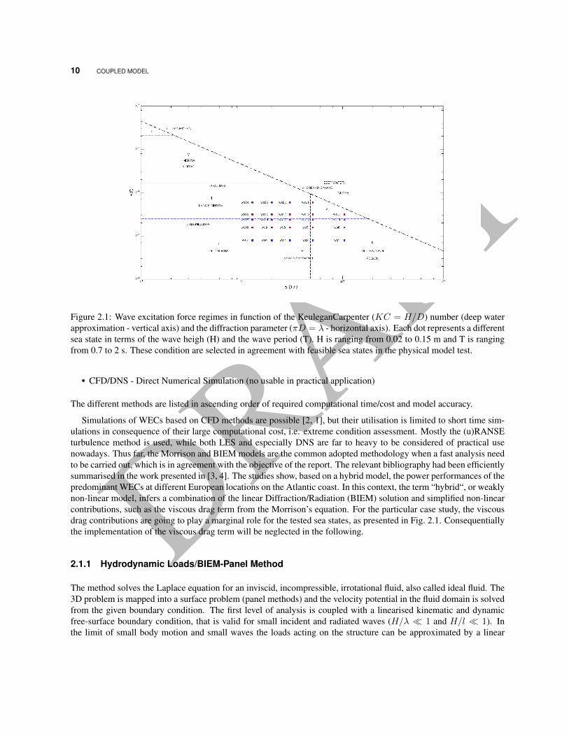
Figure 2.1: Wave excitation force regimes in function of the KeuleganCarpenter (KC = H/D) number (deep waterapproximation - vertical axis) and the diffraction parameter (πD = λ - horizontal axis). Each dot represents a differentsea state in terms of the wave heigh (H) and the wave period (T). H is ranging from 0.02 to 0.15 m and T is rangingfrom 0.7 to 2 s. These condition are selected in agreement with feasible sea states in the physical model test.

CFD/DNS - Direct Numerical Simulation (no usable in practical application)

The different methods are listed in ascending order of required computational time/cost and model accuracy.

Simulations of WECs based on CFD methods are possible [2, 1], but their utilisation is limited to short time sim-ulations in consequence of their large computational cost, i.e. extreme condition assessment. Mostly the (u)RANSEturbulence method is used, while both LES and especially DNS are far to heavy to be considered of practical usenowadays. Thus far, the Morrison and BIEM models are the common adopted methodology when a fast analysis needto be carried out, which is in agreement with the objective of the report. The relevant bibliography had been efficientlysummarised in the work presented in [3, 4]. The studies show, based on a hybrid model, the power performances of thepredominant WECs at different European locations on the Atlantic coast. In this context, the term “hybrid“, or weaklynon-linear model, infers a combination of the linear Diffraction/Radiation (BIEM) solution and simplified non-linearcontributions, such as the viscous drag term from the Morrison’s equation. For the particular case study, the viscousdrag contributions are going to play a marginal role for the tested sea states, as presented in Fig. 2.1. Consequentiallythe implementation of the viscous drag term will be neglected in the following.

2.1.1 Hydrodynamic Loads/BIEM-Panel Method

The method solves the Laplace equation for an inviscid, incompressible, irrotational fluid, also called ideal fluid. The3D problem is mapped into a surface problem (panel methods) and the velocity potential in the fluid domain is solvedfrom the given boundary condition. The first level of analysis is coupled with a linearised kinematic and dynamicfree-surface boundary condition, that is valid for small incident and radiated waves (H/λ � 1 and H/l � 1). Inthe limit of small body motion and small waves the loads acting on the structure can be approximated by a linear

DRAFTEQUATION OF MOTION 11

function of the surface elevation. Further, if steady state conditions are sought, the loads have the same frequencyas the waves that are causing them. In this framework the hydrodynamic problem can be separated in two problems,called radiation and excitation problems.

The excitation problem defines the loads exerted by the passing waves on the structure held at the equilibriumposition. Due to the linearisation of the free-surface boundary condition the wetted surface is constant. The excitationproblem is further divided in two contributions, called diffraction and Froude-Krylov. The diffraction problem is validwhen l ≥ λ, thus the wave field near the body is affected by the stationary body; so that there is no flux on the bodysurface.The Froude-Krylov problem is valid when l � λ, thus the wave filed is not affected by the presence of the body andthe velocity potential on the wetted surface equals the incident (wave) potential. The excitation loads vector (F ex) iscalculated as a summation of both diffraction and Froude-Krylov contributions. The excitation loads are defined byan amplitude and a phase shift, with respect to the incident waves, for each of the six degree of freedom (DoF) of therigid body. These are known in the offshore sector as surge (x), sway (y), heave (z), roll (Rx), pitch (Ry), yaw (Rz).Both coefficients are function of the wave frequency.

F ex(ω) = |F0

ex(ω)| ·A · <e{ei(ωt−kx+6 F0ex(ω))} (2.1)

where F0

ex are the complex excitation forces coefficients, A is the wave amplitude, ω is the circular wave frequency,t is the time coordinate, k is the wave number and x is the spacial coordinate.

The radiation problem defines the loads exerted by the body motion induced waves on the body itself, in otherwisestill water. In absence of constraints, a single rigid body freely moves in six modes, which have been defined above.Each elements of the radiation loads vector (F rad) has a term proportional to the body acceleration (Added Mass)and a term proportional to the body velocity (Radiation Damping). The coefficients are function of the body’s motionfrequency.

F rad(ω) = CM(ω)V +CA(ω)V (2.2)

where CM(ω) and CA(ω) are the added mass and radiation damping matrix respectively and V and V are the bodyacceleration and velocity vectors. Both CM(ω) and CA(ω) are square matrixes of dimension nDoF × nDoF .

Softwares like WAMIT, ANSYS AQWA and Nemoh (open-source) are solving the diffraction/radiation problemusing the panel method in frequency domain.

2.1.2 Hydrostatic Loads - Restoring

The hydrostatic loads are defined as the loads exerted by the fluid on the body due to the static pressure acting on thewetted body surface. In general the restoring forces (Fhyd) are defined as the difference between the hydrostatic loadsand the weight of the body. Under the assumption of small body motion around the equilibrium position, the restoringloads can be linearised in function of the body displacement only. For a generic rigid body the displacement (X) is a6x1 vector containing three translations and three rotations.

Fhyd = KX (2.3)

where K represents the stiffness matrix.

2.2 Equation of Motion

The hydrodynamic, hydrostatic and other external loads acting on the WEC are assembled in the equation of motionusing the Newton-Euler formulation. For a single body WEC the equation of motion defined about its centre of gravity

DRAFT12 COUPLED MODEL

(CoG) is defined as:

f = mv (2.4)τ = Icω + ω × Icω

where f is the resultant force vector, m is the mass of the system, v is the linear acceleration of the CoG of the body,t is the resultant moment vector, Ic is the body inertia matrix and ω and ω are the angular acceleration and velocity ofthe body CoG. The force and moment resultant are obtained from the summation of all the forces and moments actingon the body.

fex + frad + fhyd + fm = mv (2.5)

fex + τ rad + τhyd + τm = Icω

where fm and τm are the mooring loads. In this case no power take off system is considered. Capital and small lettersare used to distinguish between frequency and time domain variables. The gyroscopic moment (ω × Icω) may bedropped in the first step of the model definition. Due to the non-linearity of the dynamic mooring model the systemhave to be solved in time domain. The frequency dependent hydrodynamic model can be converted in time domainusing a state-space approximation or a digital time domain filter (finite impulse response filter). For a simple systemas the cylinder used in this case, both method can be adopted without no real change in the results.

2.2.1 Integration of the Mooring Loads in the Equation of Motion

The rigid body and mooring solver will exchange the following quantities: Position and velocity of the fairleads(vertex) defines the Dirichlet boundary conditions of the moving vertexes, which together with the time step lengthare the inputs to MOODY. The communication is handled via the builtin MOODY API. The time steps of the twosolver are kept different, therefore for each rigid body time step MOODY will solve a number of sub-steps. The loadsacting on the fairlead at the last time (sub-)step are used to assess the mooring loads (fm and τm). In order to evaluateposition and velocity of the fairleads in the inertial coordinate system, the position, velocity, orientation and angularvelocity of the rigid body in the global coordinate system are needed as well as the position of the fairleads in themoving coordinate system attached to the body. If pB is the position of the fairlead in the moving coordinate system,then pA and vA respectively the position and velocity of the fairlead in the inertial coordinate system can be evaluatedas

pA = ABR(θ)pB + x (2.6)

vA = ω × ABR(θ)pB + v (2.7)

where x is the displacement of the body from the equilibrium position, ABR is the rotation matrix describing the

orientation of the moving coordinate system with respect to the inertial one and θ is the triplet of Euler angles of themoving coordinate system with respect to the inertial one. Each of the mooring lines will return a force vector (fi).fm is obtained by the summation of all the contributions while τm is obtained by the summation of the single τi,defined as

τi = fi × ABR(θ)pB (2.8)

The coupled system is solved in Matlab using the built-in ode suite solver. In particular the Ode45 solver is used,which is a Runge-Kutta scheme of order four. The solver is implemented with an adaptive scheme and the time stepscannot be directly forced to stay below a given value. This creates an excessive oscillation in the mooring solution dueto the rather abrupt variation of the boundary condition tailored by the large time step. In order to solve the problemthe relative and absolute tolerance parameters have been relaxed leading to a pseudo constant time step solver.

DRAFTCHAPTER 3

COMPARISON OF THE WAVE-TO-WIRE MODEL WITHPHYSICAL TEST RESULTS

Description of the interface between the two models

Since MOODY input is defined by the position and velocity vector at the fairlead(s)

3.1 System Set-up

The set-up parameters for the numerical and physical model are summarised in Tab. 3.1 and Fig. 3.1. The Nemohsoftware was used to obtain the hydrodynamic and hydrostatic parameter of the cylinder mesh. Under the assumptionof 2D wave along the x direction it is possible to reduce the number of DoF to 3 (surge, heave, pitch). Similarly,the mooring system can be reduced to a 3D two cables set-up, forcing the force contribution along the y axis and themoment contribution around the x,z axis equal to zero.

3.2 Cable Parameter Identification

Based on the experimental results of the slack-moored buoy, a suitable set of cable parameters have been chosenfrom numerical simulations in MOODY. Due to measurement noise and large non-linearities in other tests, the regular


13

DRAFT14 MODEL VERIFICATION

Floater Geometry

Mass [kg] 3.65Moment of Inertia [kgm2] 0.1Diameter [m] 0.26Draft [m] 0.08Centre of Gravity (x,y,z) [m] [0 , 0 , -0.015]Fair Lead 1 (x,y,z) [m] [-0.13 , 0 , 0]Fair Lead 2 (x,y,z) [m] [0.1126 , 0.0650 , 0]Fair Lead 3 (x,y,z) [m] [0.1126 , 0.0650 , 0]

Cable Properties

Specific Mass [kg/m] 0.12818Length [m] 2.3Nom. Diameter [m] 0.0045Axial Stiffness [kN] 1Number of Element [-] 6Polynomial Order [-] 5

Cable Hydrodynamic Properties

Normal added mass [-] 1Tangential added mass [-] 0.08Normal drag force [-] 2.5Tangential drag force [-] 0.5

Ground model settings

Normal stiffness [kPa/m] 228Damping ratio [-] 1Friction coefficient [-] 0.3Max-friction speed [m/s] 0.1

Table 3.1: Set-up parameters

DRAFTCABLE PARAMETER IDENTIFICATION 15

Figure 3.1: Floater mesh and top and side views of the set-up. The dimensions are expressed in meter.


Figure 3.2: Comparison of the fairlead tension time series from experimental data (red), quasi-static solution (black)and MOODY solution (blue) for cable 1 and cable 2. H = 0.06m and T = 1.9 s

waves with wave height H=6 cm was chosen as validation set. The final set of cable parameters are given in Tab. 3.1.Fig. 3.2 shows the comparison of the fairlead tension time series from experimental data (red), quasi-static solution(black) and MOODY solution (blue) for cable 1 and cable 2, subject to a mild long wave (H = 0.06m and T = 1.9 s).For this long wave the loads tend to be in phase with the displacement of the fairlead and the quasi-static model providean easy and reliable solution. Measurement on cable 1 seems to be affected by a higher noise level, if compared withcable 2. Nevertheless, the results are unfiltered because by coincidence one of the eigenfrequency of the cable wasclose to the noise source frequency (around 50 Hz). Further investigation are needed to isolate and understand thisspecific behaviour.

Different consideration can be sketched from the results presented in Fig. 3.3. In this case only the results forcable 2 are presented, because of the excessive oscillation of the measurements in cable 1 - even though the sameprevious consideration about eigenfrequency of the cable could be extended for this case too. When the velocityof the boundary become important, the damping effect on the cable induces a phase-lag of both experimental anddynamic solution if compared with the quasi-static response. For the particular case presented the system is dampingdominated with a phase-lag about 90o. MOODY predict a correct phase-lag but it fails however to describe preciselythe load due to an excessive oscillation of the solution.

3.2.1 Discussion on Validity

The numerical study was made in still water, hence the effect of the water motion due to waves was not taken intoaccount. As the changing of added mass and drag force coefficients made a small change on the resulting tensionforce, it is unlikely that this affected the results significantly. It should also be mentioned that the cable was simulatedas homogenous from the anchor to the fair-lead point. In the experiments, the load cell was inserted between cable endand fair-lead, which also contributes to the uncertainty of the numerical simulation. The numerical tension forces usedfor comparison with the experiments were taken 8 cm from the end-point to compensate for this difference. Althoughthis takes care of the static offset of the tension time history, it does not correct the difference in inertia.

The ground model implementation is very important when validating numerical simulations against experimentaldata. The stiffness of the bottom and the dissipation from the cable repeatedly hitting the ground is very difficult toassess. Further, the damping of the cable tension force is very much governed by the friction model and its choice of

DRAFTCABLE PARAMETER IDENTIFICATION 17

Figure 3.3: Comparison of the fairlead tension time series from experimental data (red), quasi-static solution (black)and MOODY solution (blue) for cable 2. H = 0.06m and T = 1.3 s

Figure 3.4: Example of end-point motion sensitivity. A white-noise of 0.1 % and 0.01 % of the motion amplitude isadded to the circular motion.

parameters. As the energy dissipation from the ground interaction of the cable dominates over other damping factors,it is very difficult to choose appropriate hydrodynamic coefficients based on the experiments. In MOODY, friction ismodelled with a two-parameter viscous model based on a maximum velocity vc and a friction coefficient . To reducethe number of variables, =0.3 was chosen from literature as the friction coefficient between wet concrete and steel.

Lastly, the accuracy of the measured fair-lead motion is a key issue. The numerical simulation is very sensitiveto noise in the forced end-point motion Dirichlet condition. At this scale, the resulting tension force is then greatlydisturbed. In Fig. 3.4, a white noise disturbance amplitude has been imposed on a circular end-point motion of radiusr=3 cm and period T=3s of the seaward cable. The disturbance amplitude was 0.1 % and 0.01 % of the circular radius.


3.3 Wave-to-wire Model Validation

DRAFTBibliography

[1] Johannes Palm, Claes Eskilsson, Guilherme Moura Paredes, and Lars Bergdahl. CFD Simulation of a MooredFloating Wave Energy Converter. In European Wave and Tidal Energy Conference, EWTEC, Aalborg, 2013.

[2] Y Yu and Y Li. A RANS Simulation of the Heave Response of a Two-Body Floating Point Wave AbsorberPreprint. In International Offshore and Polar Engineering Conference, ISOPE, Maui, Hawaii, 2011.

[3] Aurelien Babarit, Jorgen Hals, and Jorgen Krokstand. Power Absorption measures and Comparisons of SelectedWave Energy Converters. In International Conference on Ocean, Offshore and Artic Engineering OMAE, pages1–10, 2011.

[4] Aurelien Babarit, Jorgen. Hals, M.J. Muliawan, A. Kurniawan, T. Moan, and Jorgen. Krokstad. Numerical bench-marking study of a selection of wave energy converters. Renewable Energy, 41:44–63, May 2012.

19