implementation of a ccd detector to dual- broadband

Implementation of a CCD detector to dual-

broadband rotational CARS and

measurements on N2O

Master of Science thesis

by Alem Kindeya

August

2010

Division of Combustion Physics

Department of Physics

Lund University

ALEM KINDEYA

MASTER THESIS REPORT

Division of Combustion Physics, Lund University

2010

ALEM KINDEYA



2010

Implementation of a CCD detector to dual-broadband

rotational CARS and measurements on N2O

Master of Science thesis

Alem Kindeya


Department of Physics

Faculty of Engineering LTH

LUND UNIVERSITY

ALEM KINDEYA



2010

© Alem Kindeya

Lund Reports on Combustion physics, LRCP-141

Lund, Sweden, August 2010

Alem Kindeya


Department of physics

Faculty of Engineering LTH

Lund University

P.O.Box 118

S-221 00 Lund, Sweden

ALEM KINDEYA



2010

Abstract

The master thesis work involved the implementation of a CCD detector to a dual-

broadband rotational coherent anti-Stokes Raman spectroscopy (DB-RCARS) setup, and

temperature measurements on N2O. This included the investigation of seven different

setting options of the detector to identify the best possible option of the camera regarding

a good precision temperature measurement. Additionally, a theoretical library for N2O at

room temperature and atmospheric pressure condition was developed. The spectroscopic

constants of the molecule are the inputs of the temperature library.

The temperature precision was found to be marginally influenced by the three basic

setting options (pre-amplifier, readout rate and binning). This indicates that it is possible

to choose any level within these setting options as long as the signal level is high (on the

order of thousand of counts). The precision was found to be independent of the binning of

pixels in the spectral dimension. The high sensitivity and high capacity output amplifiers

gave similar precision, but the signal is around five times stronger for the former

amplifier than the later. The threshold intensity above which it is possible to achieve the

smallest possible precision for the current CCD camera was identified for full vertical

binning mode to be around 1000 counts.

The measurements on N2O were made to understand the spectroscopic features of the

molecule and try to evaluate its potential for temperature measurement purposes. As a

result, the value of temperature precision was found to be better than for N2. Generally,

the N2O molecule showed a good potential for temperature measurements at room

temperature conditions.

ALEM KINDEYA



2010

ALEM KINDEYA



2010

Contents

Abstract..........................................................................................................5

Contents..........................................................................................................7

Chapter 1: Introduction...............................................................................9

1.1. Purpose of the project.......................................................... 10

1.2. General overview................................................................. 10

Chapter 2: Background Physics................................................................11

2.1. Rotational energy of molecules........................................... 12

2.2. Laser- based Combustion Diagnostic techniques............... 13

Chapter 3: Coherent anti-Stokes Raman spectroscopy (CARS)........... 14

3.1. Introduction......................................................................14

3.2. Dual-broadband rotational CARS....................................16

3.2.1. Experimental Setup of rotational CARS...... 17

Chapter 4: Andor CCD Camera.............................................................. 18

4.1. Safe Camera Operation.................................................... 19

4.1.1. Environmental Conditions................................ 20

4.1.2. Cooling............................................................. 20

4.2. Working principle of CCD detector................................ 23

4.2.1. Preamplifier gain............................................... 24

4.2.2. Readout rates..................................................... 25

4.2.3. Binning.............................................................. 26

4.3. CCD Performance........................................................... 27

4.3.1. High Sensitivity (HS) output amplifier............. 27

4.3.2. High Capacity (HC) output amplifier................ 28

Chapter 5: Experimental Work...............................................................30

5.1. Implementation of CCD Camera and testing procedure......30

5.2. N2O for temperature measurement..................................... 41

Chapter 6: Result and Discussion............................................................. 43

6.1 Detector Investigation........................................................ 43

6.1.1 Pre-amplifier gain............................................. 43

6.1.2 Read-out rates................................................... 47

6.1.3 Binning.............................................................. 50

6.1.4 Signal strength.................................................. 53

ALEM KINDEYA



2010

6.1.5 Instrument function............................................54

6.1.6 Influence of intensity on precision and SSQ.... 57

6.1.7 Comparison of FVB and Multi-track mode...... 61

6.2 Measurement on N2O......................................................... 64

6.2.1 Temperature Precision....................................... 64

Chapter 7: Summary and Outlook........................................................... 69

Reference......................................................................................................71

Acknowledgement.......................................................................................74

Appendix......................................................................................................75

ALEM KINDEYA



2010

Chapter 1

Introduction

The global energy need is expected to increase the coming decades because of many

reasons: fast economic growth of some developing countries, expansion of high level

facilities in developed countries, the global population increase in developing countries,

etc. This energy might come from different sources, but combustion has been the basic

sources of energy for many years. People were hugely dependent on combustion through

years for heating, cooking and related activities. The dependence of energy from

combustion processes is expected to increase for the future as well. This means that

combustion processes will continue to be the main source of energy despite it has

negative impact to the environment as it causes global warming which is a burning issue

this time. Figure 1.1[1]

shows a prognosis of the global energy need until 2060. Therefore,

combustion has to be efficient to generate highest possible energy from certain amount of

fuel, and to minimize environmental impact. To make a combustion process very

efficient, the process should be understood more clearly on a molecular level.

Unfortunately, this is not easy, because, the combustion process is very complicated since

it involves many elementary reactions and often has complex fluid flow. To really

understand the basic processes, there is a demand for high spatial and temporal resolution

measurements. The need for spatial resolution, temporal resolution and the importance

for non-intrusive measurement are the main reasons for the development of laser based

combustion diagnostic techniques. There are many laser based techniques which can be

used for diagnostic purposes as discussed in chapter two. The technique used in the

current study is dual-broadband rotational coherent anti-stock Raman spectroscopy (DB-

RCARS), which previously has shown to be a good technique for temperature

measurements. Nitrogen is usually probed with this technique.

Figure 1.1: Plot of global energy use as a function of years. The use of organic and fossil

fuel is expected to increase at least until 2020 and then remain relatively constant [1]

.

Organic and

fossil fuel

New and renewable

sources

ALEM KINDEYA



2010

1.1. Purpose of the project

The main aim of this project is to implement a new CCD camera to a dual-broadband

rotational coherent anti-Stokes Raman spectroscopy (DB-RCARS) setup and test options

of the CCD detector to achieve high precision temperature measurements. The second

aim is to develop a theoretical library for N2O and make temperature evaluations. This

helps to understand spectroscopic features of the molecule since the theoretical library is

developed using spectroscopic constants (rotational constant, line width, non-resonance

susceptibility, statistical weight, etc.). The current work is limited to measure room

temperature at atmospheric pressure conditions. But, the outlook of doing this

investigation is to extend the capability for temperature measurement purposes in a real

combustion environment since temperature is one important ingredient of the combustion

process which can be used as an input to model the reality.

1.2. General overview

The two main tasks which were done in this project are detector investigation and

measurement on N2O. The first task regarding detector investigation was basically the

main task of the project. The final goal of this investigation was to identify the best

possible setting option of the CCD detector to achieve a high precision temperature

measurement. Seven different investigations were made throughout the work. It is shown

that many options do not affect the precision very much. Examples of these are: pre-

amplifier setting, binning and readout rates.

The second task was code development for N2O using the spectroscopic parameters

for the molecule. The experimental data on N2O was fitted with theoretical library as

discussed in Chapter 6. The temperature was evaluated to check how good the new code

will work at room temperature condition as compared to N2 measurement. In general, the

new code looks to be promising for room temperature and atmospheric pressure

measurement. To sum up, the measurement on N2O shows that it has a potential to

measure temperature, but it needs a detailed study to investigate the diagnostic capability.

ALEM KINDEYA



2010

Chapter 2

Background Physics

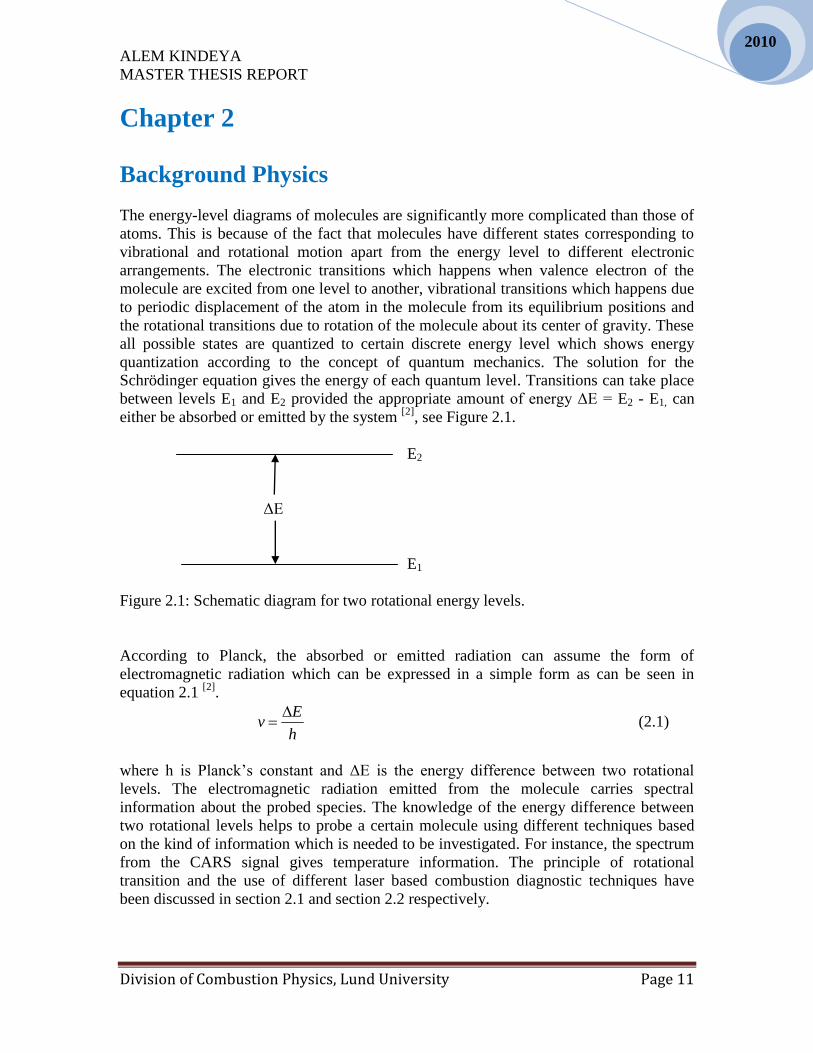
The energy-level diagrams of molecules are significantly more complicated than those of

atoms. This is because of the fact that molecules have different states corresponding to

vibrational and rotational motion apart from the energy level to different electronic

arrangements. The electronic transitions which happens when valence electron of the

molecule are excited from one level to another, vibrational transitions which happens due

to periodic displacement of the atom in the molecule from its equilibrium positions and

the rotational transitions due to rotation of the molecule about its center of gravity. These

all possible states are quantized to certain discrete energy level which shows energy

quantization according to the concept of quantum mechanics. The solution for the

Schrödinger equation gives the energy of each quantum level. Transitions can take place

between levels E1 and E2 provided the appropriate amount of energy ΔE = E2 - E1, can

either be absorbed or emitted by the system [2]

, see Figure 2.1.

E2

ΔE

E1

Figure 2.1: Schematic diagram for two rotational energy levels.

According to Planck, the absorbed or emitted radiation can assume the form of

electromagnetic radiation which can be expressed in a simple form as can be seen in

equation 2.1 [2]

.

E

vh

(2.1)

where h is Planck‟s constant and ΔE is the energy difference between two rotational

levels. The electromagnetic radiation emitted from the molecule carries spectral

information about the probed species. The knowledge of the energy difference between

two rotational levels helps to probe a certain molecule using different techniques based

on the kind of information which is needed to be investigated. For instance, the spectrum

from the CARS signal gives temperature information. The principle of rotational

transition and the use of different laser based combustion diagnostic techniques have

been discussed in section 2.1 and section 2.2 respectively.

ALEM KINDEYA



2010

2.1. Rotational energy of molecules

The rigid rotator of diatomic molecule can be given as an example to show how to model

the rotational energy, see Figure 2.2. The molecule rotating about its center of gravity has

a certain moment of inertia due to its mass. The masses m1 and m2 have moment of

inertia I1 and I2, respectively. The length (R) of the rigid bond between m1 and m2 is

given by the sum of the radius of both masses rotating about the center. The moment of

inertia of the whole system can be expressed as follows:

2 2

1 1 2 2I m r m r (2.2)

Assuming that the measurement is being made from the center of mass point for a two

mass system, then the center of mass condition can be as follows: 1 1 2 2m r m r [3], where r1

and r2 locate the masses and the center of mass lies on the line connecting the two

masses. Substituting this expression into equation 2.2, the final expression for the total

moment of inertia will be:

2 21 2

1 2

m mI R R

m m

(2.3)

where μ is reduced mass, and R is the sum of r1 and r2.

Figure 2.2: Schematic diagram of a rigid rotator rotating about the center of gravity

(center of mass) [3]

The solution for the Schrödinger equation gives the allowed rotational energy level of a

rigid diatomic molecule using the following expression [2]

: 2

2( 1) ( 1)

8J

hE J J BJ J

I (2.4)

where J = 0, 1, 2… , are rotational levels, I is the moment of inertia and B is the

rotational constant, which is typical for an individual molecule. Finally, it has to be

known that the consideration of rigid body rotator is just an approximation since all

bonds are elastic to some extent especially at high J-quantum numbers. In general, the

whole discussion of diatomic molecules could apply to polyatomic linear molecules [2]

.

But, polyatomic molecules have smaller rotational constants because of heavy mass.

ALEM KINDEYA



2010

2.2. Laser- based Combustion Diagnostic techniques

Laser-based diagnostic techniques are very crucial tools to understand the combustion

process [4]

. These can be classified as coherent and incoherent techniques. Examples of

coherent technique are polarization Spectroscopy, CARS, etc, which are basically used to

probe major species. These have strong laser like signals and they are interference

tolerant which is good, but the process is non-linear and the spectra are fairly

complicated. Incoherent techniques such as laser induced fluorescence (LIF) and Raman

scattering are linear processes, which are used to probe minor species. The good thing

with incoherent techniques is that they are intensity independent, but the large solid angle

and interference sensitive nature can be regarded as limitations. Another example of an

incoherent technique is Rayleigh scattering which is an elastic scattering process. This is

used to measure temperature if mixture composition is known. Both LIF and Rayleigh

scattering can be used for 2-D imaging. The schematic diagram of different scattering

processes is given in Figure 2.3.

Figure 2.3: Schematic diagram of Rayleigh scattering, anti-Stokes and Stokes Raman

scattering on the left side. LIF is normally emitted towards the shorter wavelength

indicated in the middle diagram. Near resonance Raman scattering is shown on the right

side [4]

The CARS technique could be used in rotational or vibrational approach depending on

which energy state or branch is probed. This technique is mostly used for temperature

measurement purposes, but it can also be used to measure concentration. In rotational

CARS process nitrogen molecule is often probed to measure temperature in a combustion

environment. The main reason is that, nitrogen is found throughout the combustion

process (from reactant to product in a fuel + air mixture) since it is an inert gas. This

helps to follow the combustion process of a flame. Air contains roughly about 78 % of

nitrogen and about 21 % oxygen, which means that the concentration of nitrogen is high

in fuel air combustion. Additionally, the fact that nitrogen is a major species makes it a

good candidate for temperature measurements using the CARS technique. The physics

behind the CARS process and its effectiveness for temperature measurements is

explained in chapter three.

ALEM KINDEYA



2010

Chapter 3

Coherent anti-Stokes Raman spectroscopy (CARS)

3.1. Introduction

Coherent anti-stokes Raman spectroscopy (CARS) was experimentally discovered at

Ford in 1965 by P.D. Marker and R.W. Terhune [5]

. The intention of their study was to

investigate different nonlinear optical effects arising from an induced optical polarization

third order in the electric field strength. The CARS process is a four wave mixing process

based on the nonlinear process via the third order susceptibility ( ). Then the CARS

signal is a result of the non-linear response of the molecule for an electric field. In other

words, three laser beams are focused to a measurement point. If the difference between

the two laser beams is in a vibrational or rotational resonance with a certain molecule, an

oscillating polarization with a Raman frequency (ωR = ω1- ω2) will be induced [6]

. Then

the CARS signal will be the sum of Raman frequency (ωR) and the frequency of the

probe beam (laser 3 at 532 nm), see Figure 3.1.

Q-branch transition S-branch transition

Figure 3.1: Energy level diagram for vibrational CARS process (a), and pure rotational

CARS process (b). Qv –branch transitions are between two vibrational levels (v → v+1)

within the same rotational states. Sv –branch transitions are between two rotational

levels (J → J+2) within the same vibrational level [6]

.

ALEM KINDEYA



2010

The induced polarization of the CARS process is a nonlinear function of the applied

electromagnetic field which is expressed as follows:

(3.1)

The third order susceptibility ( ) contains spectral (temperature) information and it is

the heart of CARS process. The susceptibility can be further divided into two terms: the

resonance susceptibility which contains the information about molecular resonances and

the Boltzmann population distribution. The second is non-resonance term which is related

to the electronic response of molecules in the probe volume [6]

.

The overall CARS signal can be expressed as [4]

:

(3.2)

where is the CARS signal frequency, , & are intensities of the three laser

beams involved in the process, is the CARS suceptibility of the medium, l is the

interaction length in the probe volume and the term in bracket represents the extent to

which the phase-matching conditions is fulfilled. If the phase-matching condition is

fulfilled, this term will assume a value of 1. The phase mismatch factor ( ) and

interaction length (l) depends on the geometry of the three mixing beams and they

determine the intensity of CARS signal (S) [4]

. Different phase matching schemes can be

employed, but there is a trade-off between spatial resolution and signal strength. The

signal strength is higher for collinear phase matching schemes, but the spatial resolution

will be lower due to extended interaction length. Thus the beams have to be crossed in

order to improve the spatial resolution. The principle of planar BOXCARS phase

matching is to arrange the three beams in such a manner that the two beams are

superimposed on top of each other and propagate parallel to the third beam. A schematic

diagram of collinear and planar BOXCARS phase matching can be seen in Figure 3.2[7]

.

Figure 3.2: Phase-matching schemes: (a) Collinear phase matching and

(b) planar BOXCARS phase matching [7]

ALEM KINDEYA



2010

3.2. Dual-broadband rotational CARS

The pure rotational CARS technique was first developed in the beginning of 1980 as an

alternative for the viberational CARS technique [8]

. But, a big improvement was

achieved when dual-broadband rotational CARS was demonstrated in 1986 [9]

. The idea

of the dual-broadband approach is to replace the two narrow beams (pump and Stokes

beams) by broadband beams from a dye laser using a red stable dye, see Figure 3.3. The

dye is pumped by Nd:YAG laser at 1064 nm which is frequency doubled to give laser

light at 532 nm. About 90 % of the light from the Nd:YAG laser is used to pump the dye

laser and the rest (10 %) with a narrow band width (FWHM = 0.7 cm-1

) is used as a probe

beam. The advantage of using broadband pump and Stokes beams is basically to achieve

a spectral averaging effect which then improves temperature precision. Additionally, the

use of a broadband dye laser gives a complete rotational CARS spectrum from a single

shot measurement. The frequency of the narrow probe beam comes out very close to the

CARS spectrum. The stray light from the 532 nm beam should then be suppressed using

an appropriate optical filter since it sometimes can be difficult to make measurements

without discriminating the stray light.

Figure 3.3: Schematic view of an energy level diagram for Dual broadband rotational

CARS process, where and are broadband lasers and 3 is a narrow band laser [6]

.

Generally speaking, a rotating molecule has a time-dependent polarizability. This means

that the molecule is Raman active, then it will give rotational CARS signals for the

transitions J→J+2 (∆J= ±2). The origin of the selection rule is from the fact that the

polarizability returns to its initial value twice for each revolution.

ALEM KINDEYA



2010

3.2.1 Experimental Setup of rotational CARS

The experimental arrangement of dual-broadband rotational CARS is shown in Figure

3.4. The Nd:YAG laser at 1064 nm, frequency doubled to produce green laser light (at

wavelength of 532 nm). Part of the green light is split-off (about 10 %) before the dye

laser to be used in the CARS experiment and the remaining green light will be used to

pump the dye laser [10]

. The dye laser peaks around 630 nm and it has bandwidth of about

250 cm-1

. There are also different optical components used in the setup such as lenses

beam splitters, filters etc.

Figure 3.4: Experimental setup of dual-broadband rotational CARS. BS, beam splitter;

D, dichronic mirror; L, lens; IP, Interaction point; BD, beam dump; and SP, short-pass

filter[10]

.

ALEM KINDEYA



2010

Chapter 4

Andor CCD Camera

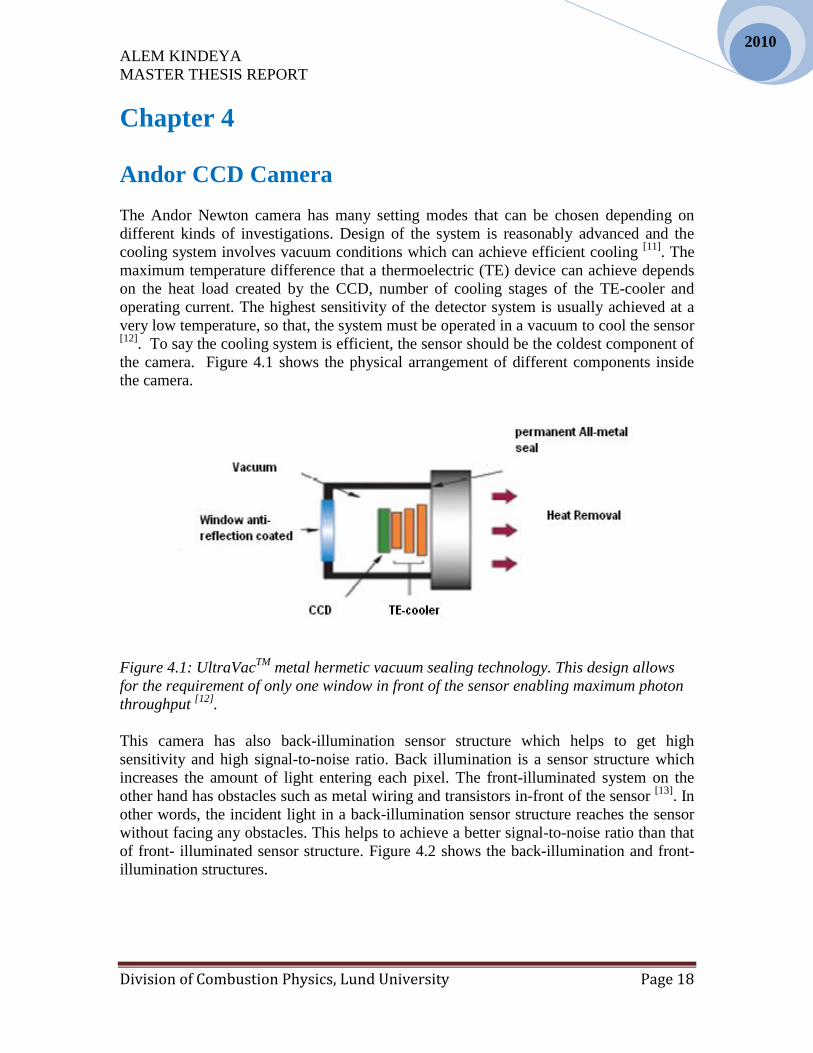
The Andor Newton camera has many setting modes that can be chosen depending on

different kinds of investigations. Design of the system is reasonably advanced and the

cooling system involves vacuum conditions which can achieve efficient cooling [11]

. The

maximum temperature difference that a thermoelectric (TE) device can achieve depends

on the heat load created by the CCD, number of cooling stages of the TE-cooler and

operating current. The highest sensitivity of the detector system is usually achieved at a

very low temperature, so that, the system must be operated in a vacuum to cool the sensor [12]

. To say the cooling system is efficient, the sensor should be the coldest component of

the camera. Figure 4.1 shows the physical arrangement of different components inside

the camera.

Figure 4.1: UltraVac

TM metal hermetic vacuum sealing technology. This design allows

for the requirement of only one window in front of the sensor enabling maximum photon

throughput [12]

.

This camera has also back-illumination sensor structure which helps to get high

sensitivity and high signal-to-noise ratio. Back illumination is a sensor structure which

increases the amount of light entering each pixel. The front-illuminated system on the

other hand has obstacles such as metal wiring and transistors in-front of the sensor [13]

. In

other words, the incident light in a back-illumination sensor structure reaches the sensor

without facing any obstacles. This helps to achieve a better signal-to-noise ratio than that

of front- illuminated sensor structure. Figure 4.2 shows the back-illumination and front-

illumination structures.

ALEM KINDEYA



2010

Figure 4.2: Front-illuminated structure in the left and, back-illuminated structure in the

right [13]

.

4.1. Safe Camera Operation

Safety is an important issue for a long lasting service of any equipment especially

electronic devices such as CCD detectors since they are more sensitive. The Andor CCD

camera is a precision scientific instrument containing fragile components such as the

sensor, which can be destroyed unless it is handled with care. Andor plc has marked a

number of screws on the detector head with red paints to prevent tampering since there

are no user-serviceable parts inside the camera, see Figure 4.3. If these screws are

adjusted for some reason, the warranty of the camera will be void [11]

. Additionally, due

attention should be given for some equipment which can cause problems for the camera.

Example: plasma source, pulsed discharge optical source, radio frequency generator and

x-ray instruments [11]

. Some of the most basic safety precautions and safe camera

operation are discussed in sections 4.1.1 and 4.1.2.

Figure 4.3: Newton CCD camera. The screws marked in red are not user-serviceable

[11]

ALEM KINDEYA



2010

4.1.1. Environmental Conditions

Conducive environmental condition can be considered as a pre-requisite for safe camera

operation. This makes the camera to function without having an external influence which

can affect the measurement results or it can further damage the detector. The Andor plc

has listed some standard environmental conditions which are important to be considered

as can be seen below [11]

:

5 V dc with 15 Watts

7.5 V dc with 30 Watts (PS-25 only)

± 25 V dc with 3 Watts

Indoor use only

Temperature 5 °C to 40 °C

Maximum relative humidity 80 % for temperature up to 31 °C, decreasing

linearly to 50 % relative humidity at 40 °C

The points listed above are some of the safety precaution which should be implemented

in any kind of measurement as far as favorable environmental condition is concerned.

Read the user manual for more detail information about safety precaution [11]

4.1.2. Cooling

Detector cooling is an important process of decreasing the temperature of the CCD chip

and to reduce the noise created due to temperature. This means, cooling the CCD detector

helps to reduce the dark signal and its associated noise. The CCD is cooled using a

thermoelectric cooler (TE). The working principle of TE cooler is actually acting as a

heat pump, i.e. it achieves temperature difference by transferring heat from its „cold side‟

(the CCD-chip) to its „hot side‟ (the built in heat sink) [11]

. This implies that the minimum

absolute operating temperature of the CCD depends on the temperature of the heat sink.

But, the failure to control the temperature could result in head overheating or it may

disable the system. Overheating may occur if either of the following occurs [11]

:

The air vents on the side of the head are accidentally blocked or there is

insufficient or no water flow.

If using air cooling and have selected deep cooling for PS-25 (the CCD

implemented in the current work). Note: Air cooling may not be possible if

the ambient air temperature is over 20 °C.

To protect the detector from overheating, a thermal switch has been attached to the heat

sink. If the temperature of the heat sink rises above 47 °C, the current supply to the cooler

will cut out and a buzzer will sound. Once the head has cooled, the cut-out will

automatically reset [11]

. This all information shows that it is very important to cool the

detector for an accurate temperature measurement and from safety point of view. The two

ways of cooling the detector in the current system are air cooling and water cooling.

ALEM KINDEYA



2010

Only air cooling has been used in the current work although the camera has both cooling

options. Air cooling is the simplest way of cooling, but it will not achieve as low

operating temperature as water cooling. Note: “The fan does not operate until the heat

sink temperature has reached between 20 °C and 22 °C. It is therefore quiet normal for

the fan not to operate when the system is first switched on [11]

”. Generally speaking,

temperature of the heat sink should be 10 °C hotter than room temperature, in order to

transfer heat efficiently to the surrounding air. The table below is a guide to the minimum

achievable operating temperature [11]

.

Table 4.1: Evacuated housing – high performance air cooling with power supply unit [11]

.

Air Temperature External PSU box

20 °C -70 °C

25 °C -68 °C

30 °C -66 °C

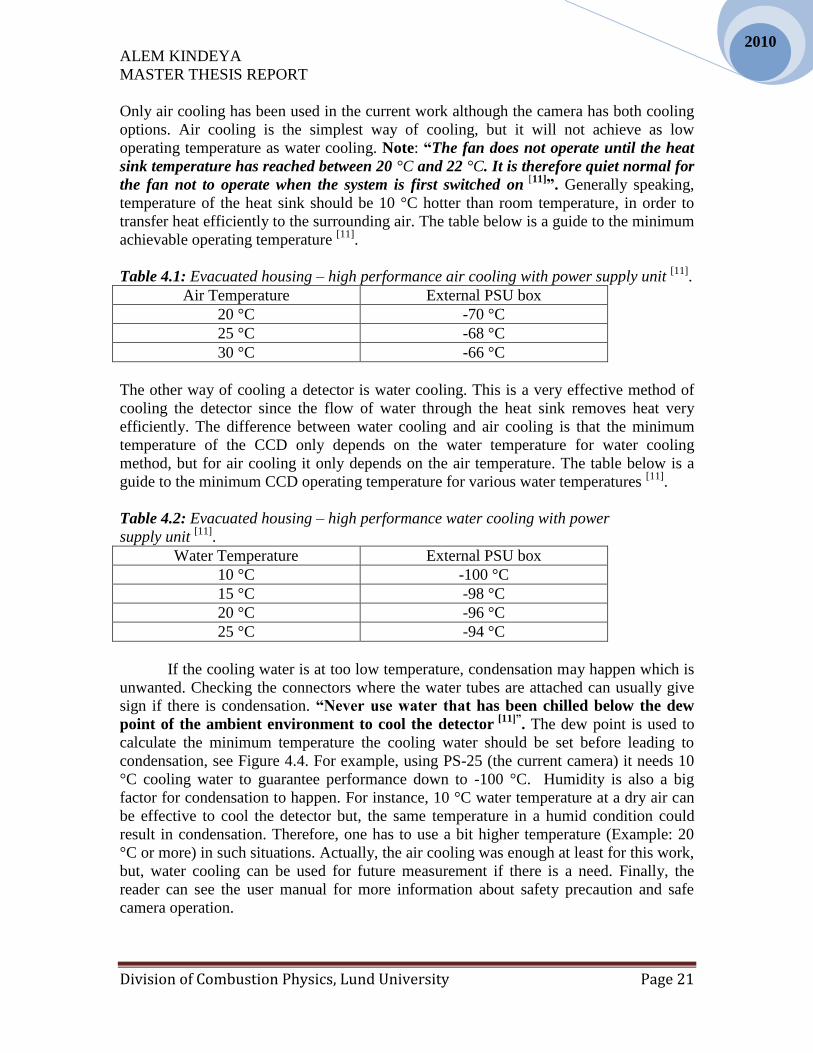
The other way of cooling a detector is water cooling. This is a very effective method of

cooling the detector since the flow of water through the heat sink removes heat very

efficiently. The difference between water cooling and air cooling is that the minimum

temperature of the CCD only depends on the water temperature for water cooling

method, but for air cooling it only depends on the air temperature. The table below is a

guide to the minimum CCD operating temperature for various water temperatures [11]

.

Table 4.2: Evacuated housing – high performance water cooling with power

supply unit [11]

.

Water Temperature External PSU box

10 °C -100 °C

15 °C -98 °C

20 °C -96 °C

25 °C -94 °C

If the cooling water is at too low temperature, condensation may happen which is

unwanted. Checking the connectors where the water tubes are attached can usually give

sign if there is condensation. “Never use water that has been chilled below the dew

point of the ambient environment to cool the detector [11]”

. The dew point is used to

calculate the minimum temperature the cooling water should be set before leading to

condensation, see Figure 4.4. For example, using PS-25 (the current camera) it needs 10

°C cooling water to guarantee performance down to -100 °C. Humidity is also a big

factor for condensation to happen. For instance, 10 °C water temperature at a dry air can

be effective to cool the detector but, the same temperature in a humid condition could

result in condensation. Therefore, one has to use a bit higher temperature (Example: 20

°C or more) in such situations. Actually, the air cooling was enough at least for this work,

but, water cooling can be used for future measurement if there is a need. Finally, the

reader can see the user manual for more information about safety precaution and safe

camera operation.

ALEM KINDEYA



2010

Figure 4.4: Plot of relative humidity versus dew point. Ambient temperature: 20 °C, 22

°C, 24 °C, 26 °C, 28 °C, 30 °C [11]

.

ALEM KINDEYA



2010

4.2. Working principle of CCD detector

The working principle of the CCD detector involves different sequential stages

throughout the data collection process. The first stage of all is the moment where the light

and matter interacts to produce charges via the process called photoelectric effect. This

is a process of generating electrons when a photon hits the semi-conductor surface (the

sensor). During this process electrons jump from the valence band to conduction band

after overcoming the potential barrier of about 1.26 eV then the electron leaves a hole

behind (at the valence band) which is considered to be a positive charge. The electron in

the valence band will now be free to move and it may also recombine with the hole, but

the electric field introduced in the CCD helps to keep both electron and the hole apart.

The electrons will be collected in a potential well which is created by the electrodes, see

Figure 4.5. During the exposure, the central electrode of each pixel is maintained at

higher potential in order to keep the electrons in the potential well. Then, the electrons

will drift away to the next electrode at the end of the exposure, due to change in potential.

By changing the potentials in a synchronized manner, the electrons will be transferred

horizontally from one pixel to the other, and it will be guided to the shift register

(counting device). Finally, the output register sends each charge package to an output

amplifier where charges are digitized and stored in to a computer hard disk. The readout

rate process is described in section 4.2.2.

Figure 4.5: The principle of photoelectric effect in a CCD detector. The charges are

collected in a potential well [14]

.

The charge transport explained above has to be digitized using an analog-to-

digital converter (A/D converter). The A/D converter is an electric circuit which helps to

convert analog signal to binary digital information (Example: counts, numbers…). The

input information to this circuit is usually continuous voltage within certain range, for

instance 0 to 10 Volts. This voltage has to be divided by the count values (2bits

) [15]

. To

make the concept understandable, an example showing the way of calculating the voltage

width and, the number of counts is given as follows. Example: A 4 bit A/D converter has

24 = 16 different counts, which ranges from 0 to 15. If the 10 Volt input is divided by 16

counts, the voltage width will be 0.625 volts. The voltage width could be different

depending on the number of bits of the analog-to-digital converter. This means that the

voltage width of a 6 bit A/D convertor with an input voltage of 10 volt is about 0.156

volts and 64 counts. Generally, the output of an A/D convertor is a binary signal, and that

ALEM KINDEYA



2010

binary signal encodes the analog input voltage, so that the output is some sort of digital

number [15]

. The explanation given so far is more of a highlight about the working

principle of an A/D converter, but the discussion may not be enough from electronics

point of view.

Coming back to the current detector, the Andor CCD has different setting modes

which can be easily manipulated to test the best possible option for a more precise

temperature measurement. The main setting options which were tested in the current

work are basically three: pre-amplifier gain, readout rate and binning. Apart from these,

there are four different modes which are tested as well despite they are interrelated

somehow with one of the three modes. The idea of the next discussion (in sections 4.2.1,

4.2.2 and 4.2.3) is mainly to give a specific explanation about the three setting options, so

that the previous discussion about the general working principle of the CCD detector will

be more understandable.

4.2.1. Preamplifier gain

A CCD can have a much larger dynamic range than can be faithfully reproduced with the

current analog-to-digital (A/D) converter. So that, to use the full capacity of the dynamic

range and to optimize the camera performance it is necessary to allow different pre-

amplifier gain [16]

. The dynamic range is a dimensionless quantity which is expressed as

the ratio of linear full well (electron) and read noise (electron). This quantity helps to

check whether A/D converter has used the full capacity of the CCD and then creates a

condition to select which pre-amplifier setting to use. For example, a certain

spectroscopic camera with model DU920N-BV has a readout noise <4e and a single pixel

dynamic range 125,000 to 1. But, a camera with 16 bit A/D converter has only 65536

different levels. This shows that the A/ D converter can not cover the full dynamic range.

So, the limited range of A/D converter effectively creates a new noise source [16]

. From

the above example, one can see that the pre-amplifier gain should be set sufficiently high

so that the overall system noise can be minimized.

In general, the function of a pre-amplifier is to amplify a low level signal to a

detectable (line level) signal prior to readout. This means that the low signal (rotational

CARS signal) coming from the source has to be pre-amplified first. This can be done by

providing some level of gain (using pre-amplifier gain setting) to make the signal

detectable then the signal will be further amplified by the output amplifier before being

transmitted to the output device, usually a computer. The sensitivity of the detector varies

depending on the choice of pre-amplifier gain values. When the gain value increases,

smaller number of electrons is needed to make the analog to digital conversion (A/D

count), which means the sensitivity of the sensor is higher. Therefore; a lot of counts will

be recorded and a very strong output signal will be achieved. Generally speaking, the pre-

amplifier gain setting significantly determines the output video signal coming out of CCD

and it helps to control the sensitivity of the detector. But, of course, a small number of

electrons are required to achieve analog to digital count (A/D count) if the gain setting is

higher (Example: x4).

ALEM KINDEYA



2010

4.2.2. Readout rates

Readout rate is the rate at which pixels (charges) are read in a sequential manner from the

shift register. The readout process is that, each set of pixels in the column of the CCD

chip will be filled by charges generated due to the photoelectric effect and then the first

set of pixels in a row will be read out, then the rest continues sequentially (the cycle starts

all over again until all the charges have been read). Figure 4.6 illustrates the readout

sequence of full resolution image which allows data to be recorded for each individual

element on the CCD-chip.

Figure 4.6: Readout mode of full resolution image. Charge in frame shifted vertically by

one row, so that the bottom row of charge moves in to the shift register [11]

.

The readout rate can be set high or low based on the need in the experiments. For

instance, high readout rates are needed when there is high repetition rate for the laser

source. The high readout rate gives large number of frame per second (image/second).

But, the readout noise is increased because of the characteristics in the read out process.

The readout time or the time it takes between two recordings by the camera should be

considered to minimize the readout noise. This means that, the readout process needs

time to transfer charges, but if the time to do this process is not enough, the readout noise

will increase.

Generally, the readout rate determines the frame rate of a certain image. This is

usually determined by pixels/second as can be seen in the equation given below

(Equation: 6.1).

Read out ratesec

image line pixel

ond image line

…………………………………… (6.1)

ALEM KINDEYA



2010

4.2.3. Binning

Binning can be defined as the process of forming super pixels. This is the sum of a

number of pixels and it will be readout as a single pixel. The horizontal and vertical

binning parameter will determine the dimension of the super pixels as can be seen in

Figure 4.7 [11]

. The Andor CCD camera software presents a selection of binning patterns

(1x1 pixels, 2x2 pixels, 4x4 pixels, 8x8 pixels and 16x16 pixels). The first pattern 1x1

pixels is the initial situation where the image is in a full resolution, but when binning

pattern 2x2 has chosen for instance, the full resolution image at 2048 pixels for the CCD-

chip of the current camera will be notionally divided in to super pixels each measure 2x2

pixel and then gives a new CCD-chip dimension of 1024 pixels. The super pixel then

provides a single signal for readout despite it contains a number of pixels.

Figure 4.7: Full resolution image with 2-dimensional pixel matrix (left image) and super-

pixel image with 2-dimensional pixels matrix (right image). The binning parameter

determines the dimension of super pixels [11]

.

The importance of binning is basically to minimize storage space, to induce faster

processing speed and to achieve higher signal-to noise ratio. The expression for the

signal-to-noise-ratio (SNR) is given in equation 6.1. This equation shows that the SNR

can be improved when the number of binned pixels (M) increases. But, it usually costs

the resolution of an image.

SNR=2

r

Mp t

Mp t MDt N

(6.1)

Where:

P is incident photon flux density

t is exposure time (integration time)

rN – Read out noise

η- Quantum efficiency

M represents number of binned pixels

ALEM KINDEYA



2010

4.3. CCD Performance

This high performance instrument has been individually built by order and tested with

Andor‟s ISO 9001: 2000 quality regime [11]

. A lot of system tests were made by the

company. An example can be the system sensitivity which is calculated in photoelectrons

per A/D count. These all investigations can help to judge the performance of the camera.

There are two output amplifier options (high capacity and high sensitivity settings) in this

CCD camera. The principle and performance of both modes are discussed in the next

sections 4.3.1 and 4.3.2.

4.3.1. High Sensitivity (HS) output amplifier

Sensitivity is a term which can be described by the quantum efficiency of a sensor. This

means that, the probability of producing photoelectrons when a photon is absorbed

describes the efficiency of the sensor. For instance, a high sensitivity sensor can achieve

single photon detection since it has very high quantum efficiency. Photons of different

wavelength have different probabilities of producing photoelectrons and this probability

is usually expressed by quantum efficiency (QE) or spectral response, which is the

number of electrons that will be produced per unit photon energy. The quantum

efficiency curves are given in Figure 4.8, for different CCD structures.

Figure 4.8: Plot of quantum efficiency (%) versus wavelength (nm). BU, back-

illuminated CCD UV enhanced 350 nm optimized; BV, back-illuminated CCD VIS

optimized; FI, front-illuminated CCD; UV, front-illuminated CCD with UV coating;

UVB, back-illuminated CCD with UV coating; BR-DD, back-illuminated deep depletion

CCD with fringe suppression; OE, open electrode CCD; BU2, back-illuminated CCD UV

enhanced, 250 nm optimized [17]

.

ALEM KINDEYA



2010

To be specific, this high resolution spectroscopic sensor has a capacity of delivering 95 %

quantum efficiency with all multi-megahertz readout. The output saturation electron for

high sensitivity and high capacity modes is 150000 and 600000 counts respectively, and

the dark current at -100 °C is about 0.00007electrons/pixel/second [18]

.

4.3.2. High Capacity (HC) output amplifier

The high capacity output amplifier is an important setting to optimize the dynamic range.

The dynamic range can be defined as the resolution of a given analog-to-digital

converter, that in most cases is given as a power of base 2, (2X). This means that an 8 bit

resolution corresponds to 256 steps (gray level), which can be used to subdivide or

convert the full scale voltage signal [19]

. The resolution directly corresponds to the

theoretical maximum limit of the converter devices, see Table 4.3. Analog-to-digital

converters have an average conversion uncertainty which can reduce the resolution for

practical application.

Table 4.3: An example showing the dynamic range for a given analog-to-digital

converter with a certain resolution [19]

Resolution (bit), X→2X

Dynamic range of analog-

to-digital conversion

(digitized steps)

Dynamic range of analog-

to-digital(A/D) conversion

in decibel(dB)

8 256 48.2

10 1024 60.2

12 4096 72.3

14 16384 84.3

16 65536 96.3

The discussion so far was concerned about the physics behind high sensitivity and

high capacity output amplifiers, but, now the focus will be on the difference between HS

and HC settings physically. The dual output amplifier allows software selection between

high sensitivity and high capacity modes of operation, so that the sensitivity and dynamic

range of capacity can be optimized to suit the operation condition. The choice of high

sensitivity mode enables the system to operate at a low noise conditions. This means that

the charge integration process enhances the sensitivity by increasing the available light

intensity to boost signal strength. This is done by extending the charge- integration time

(exposure time). But, the extended exposure time could result dark current which is a

challenge unless sufficient cooling is provided, since dark current noise increases in

proportion with exposure time. The dark noise is generated by the flow of dark current in

the silicone, and it is temperature dependent. Generally speaking, the high sensitivity

mode means the low noise condition, this will be achieved by decreasing the three

sources of noise and enhance the intensity using extended charge-integration time. The

readout noise can be suppressed by using low-speed readout and low noise circuit

technology. The shot noise can be reduced by decreasing the statistical fluctuation in the

signal using a CCD with a high Quantum efficiency (QE) [20]

. A greater statistical

fluctuation in signal means a greater shot noise.

ALEM KINDEYA



2010

On the other hand, the high capacity mode can be used to improve the dynamic range of a

sensor. There are two ways of increasing the dynamic range, the first one is, decreasing

the minimum detection limit (the smallest possible signal), and the second option is, to

increase the largest possible signal before saturation. These two possible ways can

increase the dynamic range. The largest possible signal is directly proportional to the full

well capacity of the pixel and the lowest signal is the noise level when the sensor is not

exposed to light. The full well capacity is a term which describes the capacity to hold the

electrons in each pixel that are generated from photons. After exposure of the sensor to a

light source, each pixel in a semiconductor will absorb photons and generate electrons to

be collected in a well (bucket). The level of each bucket will be assigned a value of 0 and

255 for an empty bucket (pure black) and full bucket (pure white) respectively. Pixels

with a large exposed surface can collect more photons than small pixels during the

exposure time that is needed to prevent the bright pixel from overflowing to a

neighboring pixel [21]

. If the charge flow over the neighboring pixel occurs, the so called

blooming could happen. Generally, the larger pixels have higher full well capacity which

means higher dynamic range. This implies that the high capacity setting increases

dynamic range by increasing the full well capacity. Therefore, more electrons can be

collected in high capacity mode than high sensitivity mode as it was quantitatively

described at the end of section 4.2.1.

A more accurate quantitative description of output electrons per A/D count was

made by the company (Andor plc which is the produces of the current camera with model

DU940P) as can be seen in Table 4.4. The main intention of this is to test the system

sensitivity for both high sensitivity and high capacity modes in different preamplifier

setting and various readout rates.

Table 4.4: Andor plc test of system sensitivity for HS and HC modes [11]

.

A/D Rate

(MHz All 16 bit)

Pre-amplifier

setting

High sensitivity (HS)

output electron per A/D

count

High capacity (HC)

output electron per A/D

count

3 x1 3.8 17.3

3 x2 2.0 8.9

3 x4 1.0 4.4

1.0 x1 3.9 18.0

1.0 x2 2.0 9.2

1.0 x4 0.9 4.4

0.05 x1 4.0 18.3

0.05 x2 2.0 9.4

0.05 x4 1.0 4.5

Saturation signal per pixel 83457

ALEM KINDEYA



2010

Chapter 5

Experimental Work

The main intention of the whole investigation was basically to achieve as good

temperature precision as possible by looking at different setting possibilities. The starting

point of the experimental work was to install the new CCD camera physically and also to

install the system software needed to run the camera. A number of experiments were

done in the current work to check different options of the Andor CCD camera. Pure

Nitrogen and Argon were used for the whole investigation of the detector. The N2O

measurements were also done to check the possibility of developing a good theoretical

model (Develop code using the spectroscopic constants for N2O) that can best fit with the

experimental spectrum. Additionally, it is believed that the capability of N2O library can

be extended to higher temperatures as long as accurate spectroscopic parameters are

introduced. The detailed procedure followed throughout the experimental work has been

discussed in the next sections given below.

5.1. Implementation of CCD Camera and testing procedures

The hardware implementation phase of the work includes putting the new CCD camera

and external shutter on the right position. As can be seen in Figure 5.1, a metal tube

which goes all the way to the box where the Czerny Turner spectrometer is aligned has

been mounted with the detector. The external shutter has been attached at the end of the

tube inside the box. The shutter controller kept outside the box has an on/off button to

select between keeping detector open to take a signal or closed when there is a need to

align the spectrometer or at the end of the work. This helps to use the detector safely.

Figure 5.1: Picture of general setup overview in the left, and position of CCD camera

and shutter controller on the right side (zoomed image).

ALEM KINDEYA



2010

After the implementation of the physical part, then the Andor Software package which

comes together with the CCD was installed. The software has a user-friendly interface

which enables to vary most important settings during the investigation. Then the camera

was tested for the first time to get the first Rotational CARS signal from air which was

really fascinating at least for me as a student “Yes! I know the temperature in the room…”

Some experiments were performed after making sure that the CCD works in a good way.

This was basically done to get acquainted with the system and also test how reasonable

temperatures can be measured using the new detector.

The real experiments which were done for the purpose of CCD investigation have

been performed in a more procedural manner. A total of seven different tests were made

throughout the whole project as can be seen in chapter 6 of the report. The procedure

listed below has been implemented in all investigations to minimize errors related to the

experimental procedure.

The first step in every measurement is usually taking air spectrum at room

temperature. This helps to spectrally calibrate the spectrum. The nitrogen peak in

the air spectrum at the point 123.18 cm-1

is usually taken as a reference point as

can be seen in the Figure 5.2. The only reason for this is because it is easily

identified. This peak corresponds to the S-branch transition J=14 → J= 16 in the

N2 spectrum. Therefore, the channel number (in pixels) in this specific calibration

point is an input for the FORTRAN program used to calculate temperature.

ALEM KINDEYA



2010

0 20 40 60 80 100 120 140 160 180 2000

0.1

0.2

0.3

0.4

0.5

0.6

0.7

0.8

0.9

1

X: 123.2

Y: 0.4699

Raman shift (cm-1)

Rel. I

nte

nsity (

arb

.units)

Figure 5.2: Average Air spectrum at room temperature and atmospheric pressure.

Accumulated spectrum, detector view (appearance of the spectrum in the detector without

being flipped)

The second step which has been followed was measurement on N2. In every

experiment throughout the whole work, 500 single shot nitrogen spectra were

recorded first, and then followed by 500 nitrogen background spectra (used to

subtract background from single shot spectra later in the evaluation). Then, 500

Argon spectra were collected followed by 500 Argon background spectra. The

importance of recording Argon spectra is basically to compensate the influence of

finite laser profile on the resonant spectrum of N2. This is because of the fact that

both the resonant and non-resonant spectrums are affected in the same way by the

finite laser profile of the broadband dye laser. Then the final Nitrogen spectrum

which is ready for evaluation will be in the following form:

spectra spectra

Evaluated

Spectra spectra

Nitrogen NitrogenbackgroundNitrogen

Argon ArgonBackground

…………… (5.1)

The third step in this investigation was to find the best instrument function using

the FORTRAN program (Optslit) developed by Christian Brackmann [22]

. The

FWHM values of Gauss and Lorenz line profile were found after running Optslit.

The Voigt line profile used to convolute the theoretical library of N2 is the

J (14) → J (16) in N2

ALEM KINDEYA



2010

convolution of full width at half maximum (FWHM) of Gauss and Lorenz line

profiles. Generally, the program (version by L.Martinsson, February 24, 1993)

reads a theoretical library and convolves the spectra with a Lorenz, Gauss or

Voigt slit function of specified width using Fourier transformations. A lot of

Matlab routines were also used to process the data. These Matlab codes were used

first, to generate the spectral file of single shot (SingleShot.dat format) and

accumulated shot (AccumulatedShot.dat format) which is an input for Optslit

program. Second, to process the output data received from FORTRAN program

so that temperature values and relative standard deviation (or precision) can be

calculated. Some of the Matlab codes used in the current work were the

following: To identify the reference line from air spectrum (AirSpectrum.m), to

check if the shapes of the Argon spectra were equal throughout the measurement

series (ArgonTest.m), to generate spectral data (AccumulatedShot.dat and

SingleShot.dat) as an input for FORTRAN program (printOutfile.m), to

calculate the standard deviation, Precision and Average SSQ

(CalculatePreStdAvg.m). These routines can be seen in the appendix A1, A2, A3

and A4 respectively. In fact, a lot more Matlab routines are required to make

temperature evaluation, but, the FORTRAN program is the basic one for

temperature evaluation purposes.

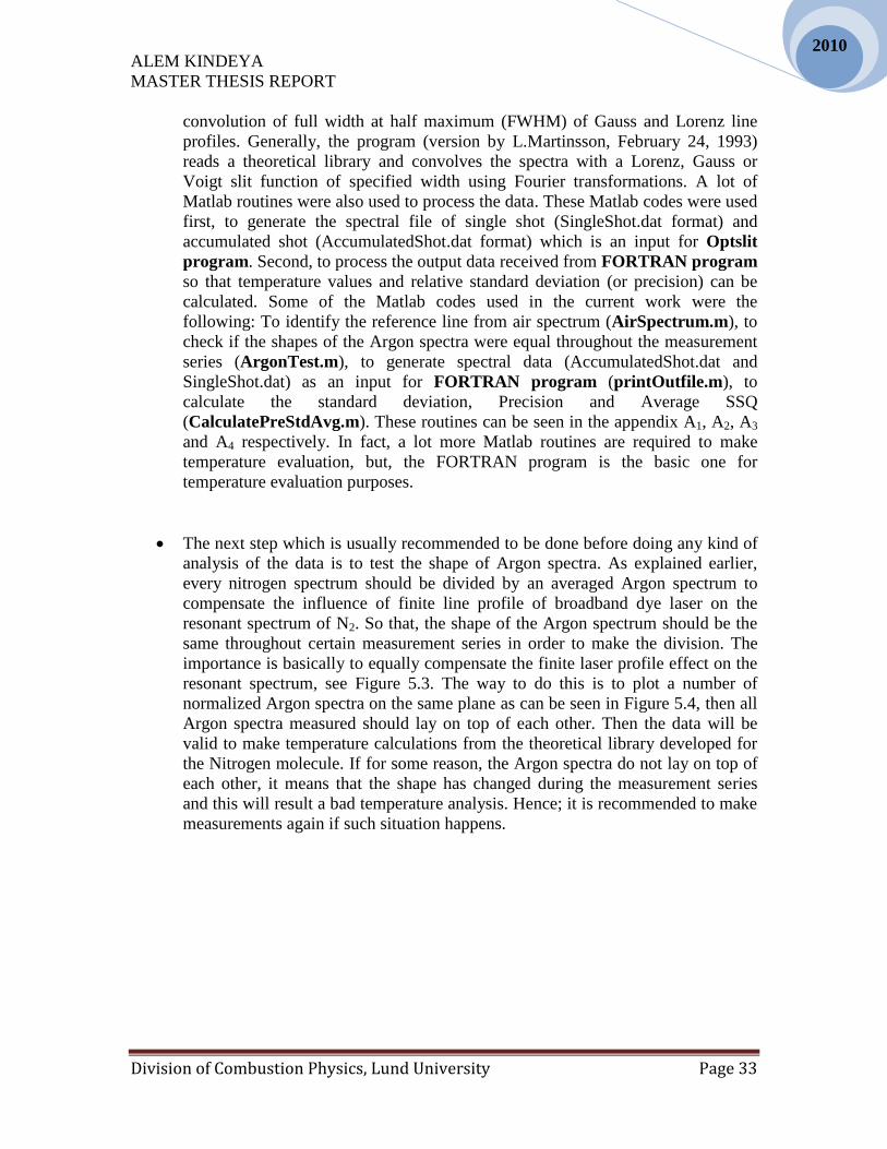
The next step which is usually recommended to be done before doing any kind of

analysis of the data is to test the shape of Argon spectra. As explained earlier,

every nitrogen spectrum should be divided by an averaged Argon spectrum to

compensate the influence of finite line profile of broadband dye laser on the

resonant spectrum of N2. So that, the shape of the Argon spectrum should be the

same throughout certain measurement series in order to make the division. The

importance is basically to equally compensate the finite laser profile effect on the

resonant spectrum, see Figure 5.3. The way to do this is to plot a number of

normalized Argon spectra on the same plane as can be seen in Figure 5.4, then all

Argon spectra measured should lay on top of each other. Then the data will be

valid to make temperature calculations from the theoretical library developed for

the Nitrogen molecule. If for some reason, the Argon spectra do not lay on top of

each other, it means that the shape has changed during the measurement series

and this will result a bad temperature analysis. Hence; it is recommended to make

measurements again if such situation happens.

ALEM KINDEYA



2010

0 50 100 150 200 250 3000

100

200

300

400

500

600

700

800

900

1000

Inte

nsity(c

ount)

Wavenumber (cm-1)

HS-X1

HS-X2

HS-X4

HC-X1

HC-X2

HC-X4

Figure 5.3: Plot of six different Argon spectra averaged over 500 spectra for six different

measurements (pre-amplifier gain: x1, x2 and x4 for each High capacity (HC) and High

sensitivity setting (HS)).

0 50 100 150 200 250 3000

50

100

150

200

250

300

350

400

450

500

Norm

aliz

ed I

nte

nsity

Wavenumber (cm-1)

HS-X1

HS-X2

HS-X4

HC-X1

HC-X2

HC-X4

Figure 5.4: Plot of six normalized Argon spectra lay on top of each other. Pre-amplifier

gain: x1, x2 and x4 have been considered for each High capacity (HC) and High

sensitivity setting (HS) options. It indicates the shape of all Argon spectra is the same. It

is good result since all Argon spectra lay on top of each other.

ALEM KINDEYA



2010

The last step of the whole process is calculation of the temperature either from the

single shot spectra or average spectrum depending on the condition. Evaluation of

averaged spectra is preferable if there is stationary condition like room

temperature measurement that has been done in the current work. This is because

the averaged spectrum has a very nice envelope function which makes

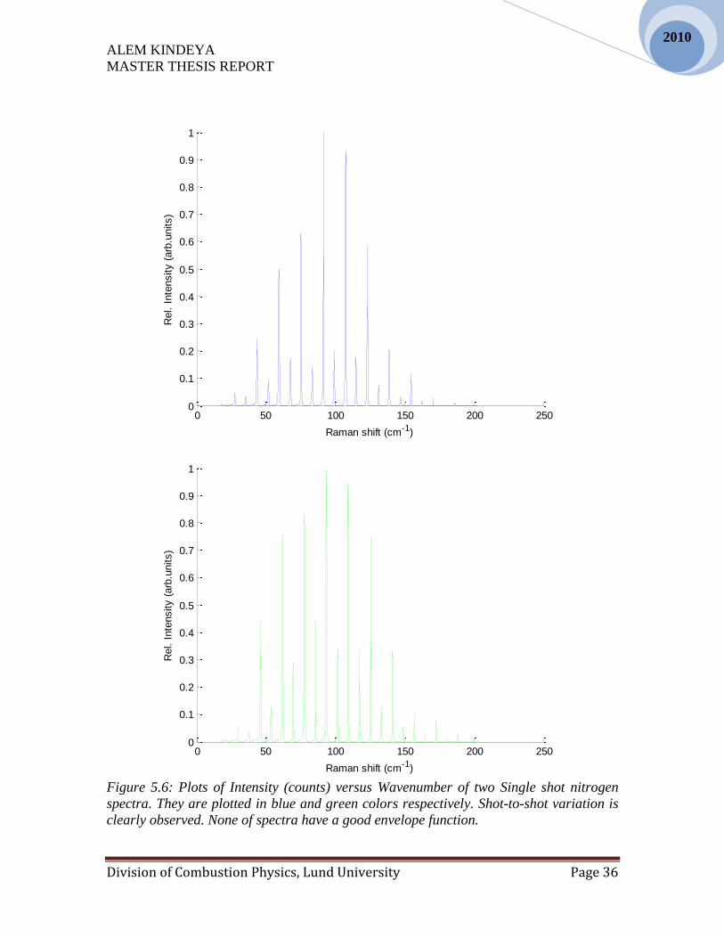
temperature calculations more precise as can be seen in Figure 5.5. However;

single shots must be evaluated in the case of non stationary conditions despite

single shot spectra have hugely varying rotational line intensities in a random

way (not a good envelop function) as can be seen in the two different single shot

spectra in Figure 5.6 plotted in blue and green colors . Evaluation of single shot

spectra is very important in cases like turbulent flames where many parameters

vary in time. In such kind of situations, it is difficult to rely only on the average

spectrum rather the single shot spectra must be evaluated. The measurement made

throughout the whole project was basically in stationary conditions, so the use of

averaging is acceptable although single shot spectrum has been evaluated as well.

In addition to this; the relative standard deviation (precision) has been calculated

for each investigation to identify the best possible way of running the camera. The

relative standard deviation is expressed as: standard deviation divided by average

temperature. This value determines how accurate the technique is on a single-shot

basis. By looking at the value for the precision, one can evaluate the quality of

certain technique since precision is a measure of how accurate the technique is on

a single-shot basis. Lower value of precision means better technique. Generally

speaking, the choice of average or single shot evaluation mainly depends on the

condition in which temperature measurement is made.

0 50 100 150 200 2500

0.1

0.2

0.3

0.4

0.5

0.6

0.7

0.8

0.9

1

Raman shift (cm-1)

Rel

. In

tens

ity (

arb.

units

)

Figure 5.5: Plot of Relative intensity (Arbitrary unit) versus Raman shift (cm

-1). Average

nitrogen spectrum over 500 spectra. The spectrum has smooth envelope function.

ALEM KINDEYA



2010

0 50 100 150 200 2500

0.1

0.2

0.3

0.4

0.5

0.6

0.7

0.8

0.9

1

Raman shift (cm-1)

Rel. I

nte

nsity (

arb

.units)

0 50 100 150 200 2500

0.1

0.2

0.3

0.4

0.5

0.6

0.7

0.8

0.9

1

Raman shift (cm-1)

Rel. I

nte

nsity (

arb

.units)

Figure 5.6: Plots of Intensity (counts) versus Wavenumber of two Single shot nitrogen

spectra. They are plotted in blue and green colors respectively. Shot-to-shot variation is

clearly observed. None of spectra have a good envelope function.

ALEM KINDEYA



2010

The difference between single shot and average spectrum is more pronounced in

case of Argon spectrum as can be seen in the Figure 5.7 plotted in red and blue colors

respectively. This shows that the shape of the Argon spectrum is very important for

temperature evaluation. Argon spectra are basically used to compensate the influence of

the finite laser profile on the resonant N2 spectra.

0 50 100 150 200 250 3000

20

40

60

80

100

120

140

160

180

200

Wavenumber(cm-1)

Inte

nsity (

Counts

)

0 50 100 150 200 250 3000

50

100

150

200

250

Wavenumber(cm-1)

Inte

nsity (

Counts

)

Figure 5.7: Plot of Intensity (counts) versus Wave number of an average Argon spectrum

(blue color) and single shot Argon spectrum (red color).

ALEM KINDEYA



2010

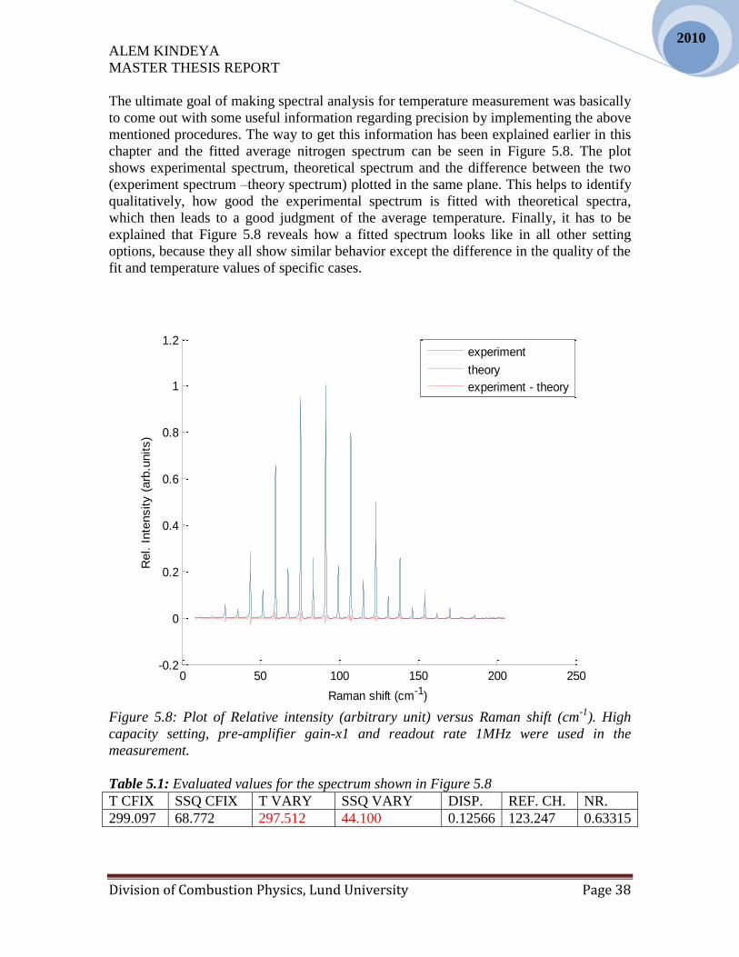
The ultimate goal of making spectral analysis for temperature measurement was basically

to come out with some useful information regarding precision by implementing the above

mentioned procedures. The way to get this information has been explained earlier in this

chapter and the fitted average nitrogen spectrum can be seen in Figure 5.8. The plot

shows experimental spectrum, theoretical spectrum and the difference between the two

(experiment spectrum –theory spectrum) plotted in the same plane. This helps to identify

qualitatively, how good the experimental spectrum is fitted with theoretical spectra,

which then leads to a good judgment of the average temperature. Finally, it has to be

explained that Figure 5.8 reveals how a fitted spectrum looks like in all other setting

options, because they all show similar behavior except the difference in the quality of the

fit and temperature values of specific cases.

0 50 100 150 200 250-0.2

0

0.2

0.4

0.6

0.8

1

1.2

Raman shift (cm-1)

Rel. I

nte

nsity (

arb

.units)

experiment

theory

experiment - theory

Figure 5.8: Plot of Relative intensity (arbitrary unit) versus Raman shift (cm

-1). High

capacity setting, pre-amplifier gain-x1 and readout rate 1MHz were used in the

measurement.

Table 5.1: Evaluated values for the spectrum shown in Figure 5.8

T CFIX SSQ CFIX T VARY SSQ VARY DISP. REF. CH. NR.

299.097 68.772 297.512 44.100 0.12566 123.247 0.63315

ALEM KINDEYA



2010

Where, T CFIX and SSQ CFIX is starting temperature and initial SSQ respectively at

the beginning of fitting. After floating both temperature, concentration, dispersion,

reference channel and non-resonance susceptibility, more accurate values for temperature

(T VARY), dispersion (DISP.), reference channel (REF. CH.) and non-resonance

susceptibility (NR.) is found as can be seen in table 5.1. The minimized parameter for the

non-linear least-squares fitting routine is the Sum-of-Squares (SSQ) [23]

. The expression

for SSQ can be seen in Equation 5.2. This is used as a measure of how good the fitting

has been made and it should be as small as possible in order to achieve a better

temperature analysis.

SSQ = 2

1

nTheory Experiment

i i i

i

W I I

(5.2)

where Theory

iI and Experiment

iI are the theoretical and experimental intensities at each point

„i‟ in the spectrum respectively, and iW is a weight factor for pixel „i‟ [23]

.

Evaluation of the average spectrum is not always enough entity to correctly determine

temperature in certain combustion environment since average data gives limited

information. Due to this reason, the single shot spectra have been evaluated for all

investigations made throughout the whole work. The individual temperatures of 500

consecutive single-shot spectra are plotted as can be seen in Figure 5.9. The standard

deviation and precision for High capacity setting (Preamplifier gain- x1, Read out rate-1

MHz) has been calculated in every analysis of the current work.

0 50 100 150 200 250 300 350 400 450 500260

270

280

290

300

310

320

330

340

Tem

pera

ture

(K

)

Number of spectra

X: 482

Y: 297

Single-shot T

Mean T

StandardDeviation

Figure 5.9: plot of Temperature (K) versus Number of spectra. The single shot

temperature with red circle shows that the non-resonance susceptibility (NR) is not fitted

for these spectra. The average temperature for 500 single-shot spectra is 297K.

ALEM KINDEYA



2010

At the last but not least, the plot of Temperature versus SSQ has been checked in every

investigation to assess the spread of the temperature of all 500 spectra, see Figure 5.10.

This kind of plot helps to see if there are some badly fitted spectra which affect the total

result of temperature precision. Actually, there is no need to remove any spectrum in the

analysis if the spectral spread is uniform on both sides of the average temperature value,

but sometimes there might be a need to remove few spectra which are less important to

the overall evaluation or because they hardly reflect the real temperature of combustion

environment. One important issue the reader has to be aware is that this Figure 5.10 is

given just to show how the spread should look like for a good distribution of single shot

spectra, but the detailed analysis is given in the result part of the report. The evaluation of

temperature for the number of spectra with SSQ<1200 gives a better precision than

evaluating the whole spectra. This shows that the spectra with SSQ >1200 might have

badly fitted spectra which negatively influence the true temperature information. Hence,

this is the way how the temperature analysis has been made throughout the whole work.

0 200 400 600 800 1000 1200 1400 1600 1800 2000270

280

290

300

310

320

330

SSQ

Tem

pera

ture

(K

)

Single-shot SSQ Vs T

5.10: Plot of Temperature versus SSQ for all 500 spectra. High capacity output amplifier

has been used.

ALEM KINDEYA



2010

5.2. N2O for temperature measurement

The Nitrous oxide (N2O) molecule (called laughing gas) was first discovered by an

English scientist clergyman Joseph Priestly in 1793[24]

. His discovery follows two steps

to create N2O. First, he had to expose ammonia nitrate (NH4NO3), and iron filings (a very

small pieces of iron which is like a powder), to heat. Second, the resulting gas, NO, was

passed through water to remove any toxic by product, see the reaction 5.2.

2NO + H2O + Fe N2O + Fe (OH)2 (5.2)

This molecule has been used for different purposes for many years, such as an anesthetic

in clinical industry and in medicine [24]

. Additionally, it has been used as a speed boost

for cars by increasing cylinder efficiency. It is characterized by non-toxic nature,

transparent look, and linear structure. It is made up of, two nitrogen and one oxygen

atoms. Having said this much about the story, and the use of N2O, it is time to explain the

potential of N2O molecule for temperature measurement purposes using CARS

technique. The measurement on N2O is the second part of the project apart from detector

investigation. All the procedures (Argon spectral shape, air reference, evaluation of the

average and single shot spectra etc) which have been implemented in the CCD

investigation using N2 were also used in this case. The main reason to use N2O for

temperature measurement purposes is to check the possibility of developing a good

theoretical model (develop code using the spectroscopic constants for N2O) that can best

fit to the experimental spectrum for room temperature condition. Additionally, this

investigation could give an indication about the potential of the molecule for some

applications of certain interest to measure temperature. In principle, N2O could give a

better precision than N2 because of the fact that the former has a lot of lines to be

evaluated while making a fit than the latter. This means that the smaller rotational

constant results in close rotational line as can be seen in Figure 5.8. The rotational

constant which is one of the factors that determines the number of spectral lines is mainly

dependent on the mass of the molecule. In this case, N2O is heavier than the N2 molecule

which means it has higher moment of inertia and smaller rotational constant. The general

expression for the rotational constant of a rigid rotator can be seen in Equation 5.3. To get

a quantitative value out of the N2O spectrum or to make temperature evaluation using this

molecule, a theoretical library has to be generated by introducing the molecular constants

for N2O. For example: rotational constant, statistical weight, line width (due to self-

broadening), rotational-vibration interaction, etc. The accuracy of temperature evaluation

depends on how precise the molecular parameters are. This makes temperature evaluation

of CARS spectrum very difficult although it gives strong laser like signal.

2 2

22 2B

I R (5.3)

where: μ - is the reduced mass, - is the reduced Planck‟s constant2

h

, R - is the

radius of the rotation axis.

ALEM KINDEYA



2010

In this work, the measurement on N2O was made at room temperature condition so that

the probability to populate higher order rotational levels is believed to be negligible. Due

to this reason, the theoretical library for N2O has been developed by only introducing

rotational constant, statistical weight, line width, some centrifugal distortion terms and

non-resonance susceptibility. According to the book by Gerhard Herzberg, F.R.S.C [25]

,

the rotational constant for N2O molecule is 0.4191 cm-1

. The statistical weights

(degeneracy factor) of all rotational levels are 1 for the nitrous oxide (N2O) molecule, and

no hyperfine structure was found for this molecule in the HITRAN data base [26]

. The

only cause for N2O line broadening in this investigation should be due to self broadening

(N2O-N2O) since pure N2O has been flowed through the measurement point. G.D.T.

Tejwani and P.Varanasi [27]

has made theoretical line width calculations in N2O-N2O.

The result for the self broadening become in good agreement with Goody‟s [28]

derived

estimate of half width for quantum numbers from m=1 to m= 60. The non-resonant

susceptibility for N2O is not a well known value. But, the investigation made at the

United Technology Center, East Hartford [29]

shows that the non-resonance susceptibility

of N2O is about double that of N2. The centrifugal distortion constant De ,αe and γe are

also calculated for N2O by Josef Pliva[30]

. Hence, all the above mentioned spectroscopic

constants have been introduced to the N2O.dat file in the Polylib. Then the theoretical

library (libN2O.lib format) has been generated in order to use for temperature evaluation

purposes in the N2O measurement. The N2O.dat file format is given in the appendix B1.

-20 0 20 40 60 80 100 120 1400

0.1

0.2

0.3

0.4

0.5

0.6

0.7

0.8

0.9

1

Raman shift (cm-1)

Rel. I

nte

nsity (

arb

.units)

Figure 5.8: Plot of Intensity (counts) versus Wavenumber (cm-1

) for N2O molecule. An

experimental spectrum averaged from 500 single-shot spectra.

ALEM KINDEYA



2010

Chapter 6

Result and Discussion

This chapter is the heart of the whole project as it includes the important analysis which

was done throughout the diploma work. As it was explained in the introductory part of

the report, this work covers two important investigations: The detector investigation

which is the major part of the work and measurement on N2O.

6.1 Detector Investigation

The aim of this investigation is basically to evaluate possible options of the Andor CCD

Camera and produce a clear procedure how to run the camera in a good way so that a

better temperature precision can be achieved for the Rotational CARS measurement

technique. All measurements regarding the detector investigation has been made using

pure Nitrogen gas and pure Argon (used to compensate the influence of finite laser

profile on the resonant spectrum of N2) at room temperature and atmospheric pressure

conditions. About seven different investigations have been performed in this part to get

all important information needed, as presented below.

6.1.1 Pre-amplifier gain

The pre-amplifier gain setting is used to amplify a low level signal to a detectable signal

prior to readout. The basic settings implemented in this investigation were: pre-amplifier

gain (x1, x2 and x4), read out rate (1 MHz at 16 bit) and full vertical binning (FVB)

mode. All 500 spectra have been evaluated in this setting. The CCD used in the current

work has an output amplifier option of high capacity and high sensitivity settings. These

two output amplifiers can be coupled with different pre-amplifier gain (x1, x2 or x4).

The two basic investigations made in this case were basically temperature precision

at different pre-amplifier gain and the change in precision of consecutive 100 spectra

from all 500 spectra collected at a time. As can be seen in these two plots (Figure 6.1 and

Figure 6.2) for high capacity and high sensitivity settings respectively, the temperature

precision is not affected much by the variation in the pre-amplifier gain. As a result, the

value of precision ranges from 2.6% to 4.4% regardless of which pre-amplifier gain used.

Additionally, it has been found that there is shot-to-shot variation among every 100

spectra of the whole 500 spectra in both settings regardless of pre-amplifier settings. To

be specific, the precision values for Pre-amp x1, pre-amp x2 and pre-amp x4 are about

0.040 ± 0.003, 0.033 ± 0.005, 0.031 ± 0.001, respectively.

From those results, one can say that, it is possible to use all three pre-amplifier

setting (x1, x2 and x4) options with out affecting much the temperature precision as long

as the CARS signal is sufficient. In other words, trying to improve temperature precision

by simply changing pre-amplifier gain will not make significant difference. Although it is

ALEM KINDEYA



2010

difficult to draw conclusion from the change in precision in every 100 spectra, the

precision is slightly better for pre-amp x4 than pre-amp x2 and pre-amp x1 seems to be

the least good. In general, the result indicates that one should use averaging over many

spectra in order to make better precision temperature measurement. Otherwise, large

variation in evaluated temperature will be found. The average values of precision for high

capacity setting (Figure 6.1) are 3.9 % for pre-amp x1, 3.5% for pre-amp x2 and 3.1% for

pre-amp x4.

0 1 2 3 4 5 6 7 80

0.005

0.01

0.015

0.02

0.025

0.03

0.035

0.04

0.045

0.05

Consecutive 100 spectra

Pre

cis

ion

pre-amp x1

pre-amp x2

pre-amp x4

Figure 6.1: Temperature precision versus consecutive 100 spectra for the high capacity

option. For every pre-amplifier setting, five measurements have been made and 100

spectra were evaluated in each case. Precision of every hundred spectra has been

calculated to check if there is shot-to-shot variation. Pre-amplifier gains x1, x2 and x4

were used.

ALEM KINDEYA



2010

Similarly, the average values of precision for high sensitivity setting (Figure 6.2)

are 3.22 % for pre-amp x1, 3.24 % for pre-amp x2, and 3.54% for pre-amp x4. This

shows that the precision improves a little with decreasing preamplifier gain.

Nevertheless, it is not very significant difference to make conclusion from this result.

0 1 2 3 4 5 6 7 80

0.005

0.01

0.015

0.02

0.025

0.03

0.035

0.04

0.045

0.05


Pre

cis

ion

pre-amp x1

pre-amp x2

pre-amp x4

Figure 6.2: Precision using different pre-amplifier settings for high sensitivity output

amplifier. For every pre-amplifier setting in high sensitivity, five measurements have

been taken and the numbers of spectra evaluated were 100 in each case.

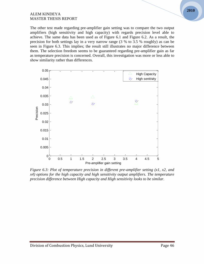
ALEM KINDEYA



2010

The other test made regarding pre-amplifier gain setting was to compare the two output

amplifiers (high sensitivity and high capacity) with regards precision level able to

achieve. The same data has been used as of Figure 6.1 and Figure 6.2. As a result, the

precision for both settings lay in a very narrow range (3 % to 3.5 % roughly) as can be

seen in Figure 6.3. This implies; the result still illustrates no major difference between

them. The selection freedom seems to be guaranteed regarding pre-amplifier gain as far

as temperature precision is concerned. Overall, this investigation was more or less able to

show similarity rather than differences.

0 0.5 1 1.5 2 2.5 3 3.5 4 4.5 50

0.005

0.01

0.015

0.02

0.025

0.03

0.035

0.04

0.045

0.05

Pre-amplifier gain setting

Pre

cis

ion

High Capacity

High senitivity

Figure 6.3: Plot of temperature precision in different pre-amplifier setting (x1, x2, and

x4) options for the high capacity and high sensitivity output amplifiers. The temperature

precision difference between High capacity and High sensitivity looks to be similar.

ALEM KINDEYA



2010

6.1.2 Readout rates

Readout rate is the rate at which pixels are read in a sequential manner from the shift

register. The purpose of this investigation was to check what happens to the precision if

the readout rate is varied, to see if the readout rate can really change the precision in

consecutive 100 spectra and also to make comparison between the precision levels of

high capacity and high sensitivity output amplifier settings at different readout rates. The

temperature precision for different readout rates (3MHz, 1MHz and 0.05 MHz) have been

investigated in similar way as the case of Pre-amplifier gain which was discussed in

section 6.1.1. The pre-amplifier setting used was x1 in a full vertical binning (FVB)

mode. The whole analysis was done for both high capacity and high sensitivity output

amplifier settings. The plot of precision as a function of consecutive 100 spectra for all

three readout rates is shown in Figure 6.4 for high capacity output amplifier setting. The

precision lays in the range of 3 % to 4 % for all readout rates. The difference in precision

between consecutive 100 spectra was also evident in all of the three cases. However; it is

still difficult to prefer one readout rate from the other as far as temperature precision is

concerned. This is because, all readout rates shows a variation within the given range

regardless of choosing high or low rate. The other important issue which should be

realized is that, the shot-to-shot variation of consecutive 100 spectra is not affected much

by the readout rate.

0 1 2 3 4 5 6 7 80

0.005

0.01

0.015

0.02

0.025

0.03

0.035

0.04

0.045

0.05


Pre

cis

ion

1 MHz

3 MHz

0.05 MHz

Figure 6.4: Plot of precision versus consecutive 100 spectra for different readout rates

(1MHz, 3MHz and 0.05MHz and high capacity setting). FVB mode and x1 pre-amplifier

setting have been used in this investigation. All 500 in a sequence of 100 each have been

evaluated.

ALEM KINDEYA



2010

A similar investigation has been made for the high sensitivity output amplifier as can be

seen in Figure 6.5. The precision varies in the range of 2.7 % to 4.1 % for all readout

rates. This shows that the conclusion will be quite similar with high capacity setting case.

From those two investigations, it can be concluded that the influence of choosing

different readout rates is very small or may be negligible for the temperature precision.

0 1 2 3 4 5 6 7 80

0.005

0.01

0.015

0.02

0.025

0.03

0.035

0.04

0.045

0.05


Pre

cis

ion

1 MHz

3 MHz

0.05 MHz

Figure 6.5: Plot of precision versus consecutive 100 spectra for different readout rates

(1MHz, 3MHz and 0.05MHz) and high sensitivity setting. FVB mode and x1 pre-amplifier

setting have been used in this investigation. All 500 in a sequence of 100 each have been

evaluated.

ALEM KINDEYA



2010

The third investigation was intentionally made to check the difference in precision when

using high capacity or high sensitivity setting as can be seen in Figure 6.6. It then came

out with a result which shows that a selection freedom is still granted specially at high (3

MHz) and low (0.05 MHz) readout rates. At 1 MHz the high capacity setting looks to

have better precision than high sensitivity, but it is too difficult to make conclusion based

on this point (the range of precision is 3.1 % to 3.7%). Therefore; it can be concluded that

both output amplifier settings are almost equally good to make temperature measurement

as long as precision in the main concern.

Figure 6.6: Plot of precision versus readout rate for both high sensitivity and high

capacity settings. The numbers of spectra evaluated were on average: 400 spectra for

high capacity and 350 spectra for high sensitivity setting since only SSQ<600 were

evaluated.

0 0.5 1 1.5 2 2.5 3 3.5 4 0

0.005

0.01

0.015

0.02

0.025

0.03

0.035

0.04

0.045

0.05

Readout rate

Precision

High Capacity-x1

High Sensitivity-x1

ALEM KINDEYA



2010

6.1.3 Binning

Binning is a process of forming a super pixel as it was explained in chapter 4. The

objective of this analysis is to check the influence of horizontal binning to precision and

SSQ. The setting implemented in this case was: High Sensitivity output amplifier,

preamplifier gain-x1, read out rate-1MHz at 16 bit. This setting has been used equally

to all binning patterns (bin 1, bin 2, bin 4, and bin 8). Figure 6.7 shows that the

temperature precision is in the range of 2.7 % to 3.2 % for the horizontal binning options

bin 1, bin 2, bin 4, and bin 8. But, it is difficult to draw conclusion about that, since the

temperature precision does not seem to have a big correlation with binning. Therefore,

one can use any binning option as far as precision is concerned.

0 1 2 3 4 5 6 7 8 9 100

0.005

0.01

0.015

0.02

0.025

0.03

0.035

0.04

Horizontal binning

Pre

cis

ion

Figure 6.7: Plot of Precision versus horizontal binning (bin 1, bin 2, bin 4, and bin 8).

The precision looks to be rarely affected by binning. 500 single shot spectra have been

evaluated in this case.

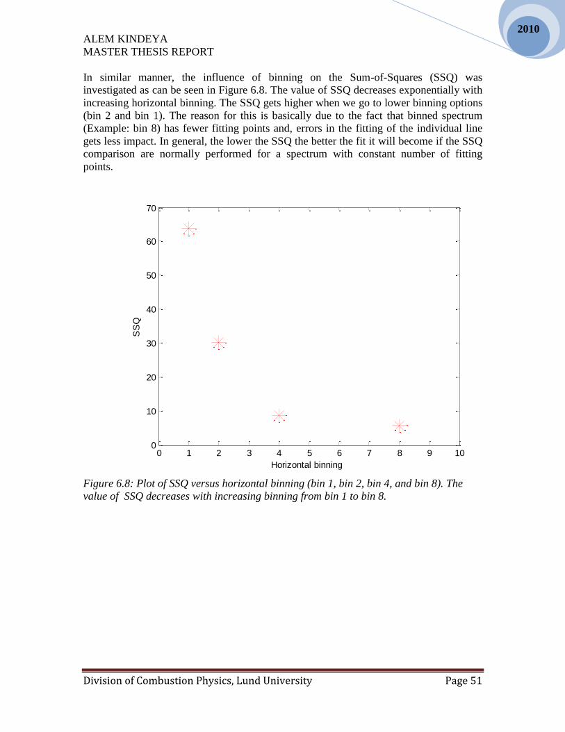
ALEM KINDEYA



2010

In similar manner, the influence of binning on the Sum-of-Squares (SSQ) was

investigated as can be seen in Figure 6.8. The value of SSQ decreases exponentially with

increasing horizontal binning. The SSQ gets higher when we go to lower binning options

(bin 2 and bin 1). The reason for this is basically due to the fact that binned spectrum

(Example: bin 8) has fewer fitting points and, errors in the fitting of the individual line

gets less impact. In general, the lower the SSQ the better the fit it will become if the SSQ

comparison are normally performed for a spectrum with constant number of fitting

points.

0 1 2 3 4 5 6 7 8 9 100

10

20

30

40

50

60

70

Horizontal binning

SS

Q

Figure 6.8: Plot of SSQ versus horizontal binning (bin 1, bin 2, bin 4, and bin 8). The

value of SSQ decreases with increasing binning from bin 1 to bin 8.

ALEM KINDEYA



2010

The results from the four different binning options (bin 1, bin 2, bin 4 and bin 8) are

plotted in Figure 6.9. The numbers of spectra are 500 for each binning option. The

distributions indicate that the SSQ value for bin 1 > bin 2 > bin 4 > bin 8. This helps to

understand what happens to the spectral fit as the horizontal binning increases.

0 200 400 600 800 1000 1200 1400260

270

280

290

300

310

320

330

SSQ

Tem

pera

ture

bin 1

bin 2

bin 4

bin 8

Figure 6.9: Plot of Temperature versus SSQ for different binning options (bin 1, bin 2,

bin 4 and bin 8). 500 spectra were evaluated for each case.

ALEM KINDEYA



2010

6.1.4 Signal strength

High signal-to-noise ratio is usually needed to extract useful information from

measurements. The CARS signal strength is actually good enough for measurement

purposes since it is a laser like coherent signal which is created by implementing the

phase matching conditions for three different lasers focused to a point. The rotational

CARS signal strength could be affected by the use of some optical equipment such as the

filter which is basically used to block the stray light from the laser source at wavelength

532nm. This investigation regarding signal strength is concerned to verify which output

amplifier should be used if one needs to have a strong output signal from the same input.

The Andor CCD camera used in the current work has two options for the output amplifier

(High sensitivity and High capacity) and both have three possible setting options (x1, x2

and x4) as can be seen in Figure 6.10. A high sensitivity (x4) and high capacity (x4) CCD

setting means high quantum efficiency sensor with large exposure time, and high

dynamic range respectively. The signal strength for high sensitivity output setting is a bit

more than five times as big as the signal strength of high capacity setting, see Figure

6.10. This implies that, the high sensitivity output amplifier setting is more preferable

than high capacity setting as far as signal strength is concerned.

0 1 2 3 4 5 60

0.5

1

1.5

2

2.5

3

3.5x 10

4

Pre-amplifier gain

Sig

nal str

ength

High capacity

High sensitivity

Figure 6.10: Plot of signal strength versus pre-amplifier gain(x1, x2 and x4) for High

capacity and high sensitivity settings. The signal strength for the high sensitivity is twice

as big as High capacity setting as can be seen in the figure.

ALEM KINDEYA



2010

6.1.5 Instrument function

The instrument function used in the current work was a Voigt line profile as it was

explained in the experimental part of the report. This line profile is basically the

convolution of Gauss and Lorenz line profiles. An investigation was made to check the

influence of resolution on the line profiles when the position of the CCD detector goes

away from the point of focus. By changing the CCD detector position the width of the

instrument function varied as can be seen in Figure 6.11. The full width at half maximum

(FWHM) value for both Gaussian and Lorentzian line profiles was evaluated from the

instrument function at each measurement positions. From this figure, one can see that the

FWHM of Gaussian line profile increases with increasing the distance while the FWHM

for Lorentzian line profile remains reasonably constant. This shows that the change in

resolution of CCD camera is much correlated with a Gaussian line profile. So, the Voigt

profile should be the convolution of bigger gauss profile and reasonably constant

Lorentzian line profiles.

0 1 2 3 4 5 6 7 80

0.1

0.2

0.3

0.4

0.5

0.6

0.7

0.8

0.9

CCD camera position

Fitting p

ara

mete

r

Gaussian profile

Lorentzian profile

Figure 6.11: Plot of the fitting parameters of the instrument function versus CCD camera

position. As we go farther from focus the resolution decreases and the lines will be

broader. The FWHM of Gauss line profile increase with increasing distance while the

Lorentzian line profile remains constant. This shows that it is necessary to increase the

FWHM of gauss line profile when the lines are broader to make a good fit.

ALEM KINDEYA



2010

In similar manner, the temperature precision and SSQ were checked at different

measurement positions of the detector. This helps to figure out the correlation of detector

resolution with precision and SSQ. As a result, the change in distance (and thereby

resolution) of the camera does not affect the temperature precision and SSQ as can be

seen in Figure 6.12 and Figure 6.13 respectively. The average precision as a function of

distance is about (3.3 ± 0.1) % and the average SSQ value as a function of CCD position

is in the range 301- 304.

0 1 2 3 4 5 6 7 80

0.005

0.01

0.015

0.02

0.025

0.03

0.035

0.04

CCD camera position

Pre

cis

ion

Figure 6.12: Precision versus Measurement position for SSQ < 1000. The precision is

not affected much in this range of CCD position as long as all temperatures values with

SSQ<1000 are considered.

ALEM KINDEYA



2010

0 1 2 3 4 5 6 7 80

50

100

150

200

250

300

350

400

CCD camera position

SS

Q

Figure 6.13: Average SSQ versus Measurement position for SSQ < 1000. The SSQ seems

to be constant in all positions of the x-axis within the limit given above.

Table 6.1: Number of evaluated spectra, measurement positions & Fitting parameters

used for the spectrums shown in Figure 6.11, Figure 6.12 & Figure 6.13

Spectra

evaluated

Position

(mm)

Precision

Average

SSQ

Fitting parameters

Gauss

profile

Lorenz

profile

487 33 0.0332 303.0722 0.325 0.125

493 35 0.0340 301.9624 0.325 0.125

494 37 0.0334 303.3468 0.5 0.1

499 39 0.0329 302.8662 0.575 0.125

500 41 0.0328 302.5933 0.6 0.175

482 43 0.0332 302.0747 0.725 0.15

ALEM KINDEYA



2010

6.1.6 Influence of intensity on precision and SSQ

The relative standard deviation (here called precision) is an important quantity which is

used to evaluate the technique implemented in a certain measurement, and the SSQ also

indicates how good an experimental spectrum is fitted with theoretical spectrum. The

idea of this investigation was to identify the minimum peak intensity (counts) that must

be achieved on the detector to get rid of detector noise contribution to the overall

precision and to check the correlation between peak intensity value and SSQ. This means

that the intensity above the minimum value does not change much the precision and SSQ

while intensity less than the minimum value will give worse temperature precision and

SSQ values. Figure 6.14 shows that, minimum peak intensity about 1000 counts is

needed to keep the precision as good as possible for the full vertical binning mode (FVB).

Peak intensity value less than about 1000 counts results in worse precision.

101

102

103

104

0

0.01

0.02

0.03

0.04

0.05

0.06

0.07

0.08

Average intensity (counts)

Pre

cis

ion

FVB mode

Figure 6.14: Precision versus Average intensity for the FVB mode. 500 single shot

spectra were evaluated. The temperature precision improves with increasing intensity

until 1000 Counts. And the precision shows the same result with in the intensity range of

1000 up to the maximum intensity before saturation.

ALEM KINDEYA



2010

In similar manner, the average SSQ was plotted as function of average peak signal

intensity as can be seen in Figure 6.15. The minimum peak intensity needed to keep the

SSQ value relatively constant is about 1000 counts. The SSQ value remains relatively

constant or decreases slightly at higher intensity (greater than 1000). The last point with

intensity 32055 counts has SSQ value of about 1014. This could be due to saturation of

the detector.

101

102

103

104

105

0

500

1000

1500

2000

2500

3000


Avera

ge S

SQ

FVB mode

Figure 6.15: Average SSQ versus Average peak signal intensity for FVB mode. 500

single shot spectra were evaluated. The SSQ value of FVB is lowered with increasing

signal intensity until it reaches around 1000 counts, then it remains almost constant at

any maximum intensity before saturation.

ALEM KINDEYA



2010

The other investigation made regarding binning options was the multi-track mode. This

mode is a full vertical binning of a limited number of rows on the CCD chip containing

the signal (pixels containing the CARS spectrum). The main idea of doing that was to

investigate its effect on precision and SSQ. In order to do that, a certain track which

contains the CARS spectrum was selected from the CCD chip to run the camera in a

multi-track mode. As a result, the spectrum was found in an area of around 25 vertical

pixels (2048x25). A similar investigation was implemented to multi-track mode as of

FVB mode. The minimum peak intensity or threshold looks to be difficult to identify in

multi-track mode as can be seen in Figure 6.16. The worst precision found in this case

was the first point at around 30 counts which is very low intensity. Hence, it is only

possible to say that the precision shows improvement with increasing intensity,

otherwise, it is hard to put a certain threshold.

101

102

103

104

105

0

0.01

0.02

0.03

0.04

0.05

0.06

0.07


Perc

isio

n

Multi-track mode

Figure 6.16: Precision versus average signal intensity for the multi-track mode. 500

single shot spectra were evaluated. The precision shows slight improvement with

increasing average intensity. However, the temperature precision will be worst for a

signal less than or equal to 180 counts due to lower signal.

ALEM KINDEYA



2010

The plot of average SSQ versus peak intensity given in Figure 6.17 indicates that the fit is

getting worse for an intensity value less than about 1000 counts. The average intensity

above 1000 counts gives relatively constant value of SSQ. Generally, the precision

decreases with increasing number of counts for a multi-track mode.

101

102

103

104

105

0

500

1000

1500

2000

2500

3000


Avera

ge S

SQ

Multi-track mode

Figure 6.17: Average SSQ versus Average intensity for the Multi-track mode. The curve

show that the average SSQ for 500 single shot spectra decreases with increasing average

intensity up to around 1000 counts. Above 1000 counts, the average SSQ is relatively

constant except for the highest average intensity. But, this increase in SSQ is expected

due to detector saturation.

ALEM KINDEYA



2010

6.1.7 Comparison between Full vertical binning and Multi-track modes

The main idea of this comparison is to investigate the influence of CCD noise

contribution from the pixels which do not have spectral information. In other words, the

CCD chip used in the current work has 2048x512 pixel sizes but, the rotational CARS

signal only covers around 25 pixels (like 2048x25). In such cases, the full vertical

binning (FVB) will simply add noise to the overall signal. However, multi-track mode

can neglect those pixels since it only bins the selected pixel. In principle, multi-track

mode could give a better precision if CCD readout noise is dominating factor for the

overall noise contributions. Figure 6.18 shows that the temperature precision of both FVB

and multi-track modes are about the same especially at high enough intensity (greater

than 1000). The FVB mode gives relatively worse temperature precision for intensity less

than about 200 counts. This shows that multi-track mode is preferable at low intensity

conditions since the CCD readout noise contribution could be bigger in such situations.

101

102

103

104

105

0

0.01

0.02

0.03

0.04

0.05

0.06

0.07

0.08


Pre

cis

ion

FVB mode

Multi-track mode

Figure 6.18: Precision of measurements using multi-track and FVB modes as a function

of average intensity. Both have almost similar precision levels for intensity values greater

than or equal to 200 counts. For low intensity multi-track mode looks to be more

preferable than FVB mode. This could be due to the fact that there will be noise

contribution from some of the pixel in the FVB which were removed in the multi-track

mode.

ALEM KINDEYA



2010

A similar comparison has been made to evaluate the difference in SSQ between FVB and

multi-track mode as can be seen in Figure 6.19. The average SSQ decreases with

increasing peak intensity. This could mean that it is possible to use both FVB and multi-

track modes in that region as far as SSQ is concerned, but one has to be careful when

choosing highest possible intensity which can give an improved precision before

saturation. Because, a very high signal could saturate the detector and it may result in

worse SSQ as can be seen in the last measurement points. In general, multi-track mode

looks to be preferable for low intensity signal in comparison with FVB mode.

101

102

103

104

105

0

500

1000

1500

2000

2500

3000


Avera

ge S

SQ

FVB mode

Multi-track mode

Figure 6.19: Plot of average SSQ versus average intensity (counts).Both the FVB and

multi-track modes have similar values regarding SSQ for signal intensity greater than

1000 counts. The SSQ value is very sensitive for an intensity value of less than 1000

counts

Table 6.2: High and low signal intensity for both FVB and multi-track modes. At low

signal, the precision for multi-track mode is better than FVB mode. But, at high enough

signal level, both can be used or FVB binning may be a bit better than multi-track mode.

High signal Intensity

(Counts)

Low signal Intensity

(Counts)

FVB mode 0.0303 9305 0.0502 263

Multi-track mode 0.0341 9740 0.0404 309

ALEM KINDEYA



2010

To sum up, the relative standard deviation (called precision in our case) is a measure of

dispersion or scattering around the mean value. The smallest the value of precision the

better the technique will be and the higher value of precision means the worse technique.

The value of precision achieved in the present study regarding detector investigation was

found to be 3% - 4% on average (which means 8-11K temperature roughly). Previous

studies of DB-RCARS thermometry shows that the value of precision achieved at room

temperature condition was found to be 4% - 5% [31]

. Similarly, standard deviation of 5-6K

(which means that a precision of about 1.7% - 2% roughly) was achieved using modeless

dye laser at room temperature [32]

. The above result indicates that the temperature

precision achieved in the current investigation is reasonably good as compared with the

precision of DB-RCARS at room temperature with a multimode Nd:YAG laser and a

conventional dye laser. But, the investigation by F. Vestin, M. Afzelius and P-E

Bengtsson using modeless dye laser lowered the standard deviation of conventional dye

laser by 50% [32]

.

ALEM KINDEYA



2010

6.2 Measurement on N2O

Nitrous oxide (N2O) has been used for different purposes like medicine, as it has been

explained in chapter 5. But, it is not used for temperature measurement purposes in

combustion applications, since it should be noted that the concentration of N2O is very

low in hydrocarbon combustion which makes it difficult to probe the molecule via the

CARS technique. Due to this reason, there is almost no chance to follow the combustion

process by probing N2O. The spectroscopic constants of this molecule are not well known

quantities as compared to nitrogen (N2). But, the accuracy of temperature evaluation via

CARS technique depends on the accuracy of spectroscopic constants of the molecule

which are inputs to develop the theoretical library. Generally speaking, the idea of this

investigation is just to test N2O molecule for temperature measurement at room

temperature and atmospheric pressure conditions. The detail analysis is described in

section 6.2.1.

6.2.1 Temperature Precision

The temperature precision was calculated in this investigation for both N2O and N2

molecules. The measurement was made at the same conditions for both molecules (pre-

amplifier gain x1, readout rate 1 MHz at 16 bit and high sensitivity output amplifier

settings). The fitted spectrum of the N2O molecule shows that the theoretical library

developed for this molecule works quite well at room temperature conditions, but, it can

be improved even more until a more reliable temperature value is measured, see Figure

6.20.

-20 0 20 40 60 80 100 120 140-0.2

0

0.2

0.4

0.6

0.8

1

1.2

Raman shift (cm-1)

Rel. I

nte

nsity (

arb

.units)

experiment

theory

experiment - theory

Figure 6.20: Plot of the N2O fitted spectrum averaged over 500 spectra.

ALEM KINDEYA



2010

Although the N2O library works at room temperature conditions, the evaluated average

temperature is very high (317.805 K) as compared to room temperature condition which

is roughly about (296 ± 2) K , see table 6.4.


T CFIX SSQ CFIX T VARY SSQ VARY DISP. REF. CH. NR.

277.447 183.792 317.805 25.978 0.12656 61.139 1.86812

This higher evaluated temperature of N2O could be due to different reasons. For instance,

the Raman line widths of the molecule can influence the temperature unless a very

accurate value is introduced to the library. The line widths of N2O [27]

and N2 [33]

due to

self broadening are given in Figure 6.21 for the rotational quantum number (J=1 to J=60).

By looking at this figure, one can see that there is a significant difference between the

two molecules. This implies that a less accurate line width parameter could bias

temperature information by giving high or lower temperature than it should be.

Therefore, a more accurate line width value is needed in the current work as well to get

the temperature lower than the already evaluated value.

0 10 20 30 40 50 600

0.02

0.04

0.06

0.08

0.1

0.12

Rotational level (J)

Ram

an lin

e w

idth

N2O-N2O

N2-N2

Figure 6.21: Plot of line width versus rotational quantum number (J=1 to J=60) for the

N2O- N2O [27]

(blue color) and N2- N2 [33]

(red color) self broadening.

ALEM KINDEYA



2010

The good thing with temperature measurement on N2O is actually, its high accuracy

measurement capability at room temperature. In chapter 5 of the report, it has been

explained that the small rotational constant of this molecule can be considered as one

reason for the existence of many rotational lines which gives an extra advantage to make

a fit. This idea looks to be correct according to the evaluation made in the current work.

Smaller value of relative standard deviation (precision) means that the temperature

precision is higher. The standard deviation, mean temperature and single shot

temperature distributions of 500 single shot spectra for N2O are plotted as can be seen in

Figure 6.22. The calculated values of standard deviation, precision and average SSQ are

given in table 6.5.

0 50 100 150 200 250 300 350 400 450 500312

314

316

318

320

322

324

326

328

X: 482

Y: 320.4

Tem

pera

ture

(K

)

Number of spectra

Single-shot T

Mean T

StandardDeviation

Figure 6.22: Plot of Temperature (K) versus Number of spectra. The average

temperature for 500 single-shot spectra is 320.4K.


Standard deviation Precision Average SSQ for single shot spectra

2.3964 0.0075 151.0061

ALEM KINDEYA



2010

Similarly, temperature measurement on N2 was made for a comparison purposes. The

evaluated temperature of N2 molecule is lower than that of N2O, and it is closer to room

temperature conditions. This could be because of the fact that the N2 library was

developed using relatively accurate spectroscopic parameters. That‟s why it has been

always said that the precision of temperature evaluation using CARS technique is

dependent on the accuracy of spectroscopic parameters. The averaged spectrum of N2

molecule fits very well with theoretical spectrum as can be seen in Figure 6.23. The

evaluated values of the fitted spectrum are given in table 6.6.

0 20 40 60 80 100 120 140 160 180-0.2

0

0.2

0.4

0.6

0.8

1

1.2

Raman shift (cm-1)

Rel. I

nte

nsity (

arb

.units)

experiment

theory

experiment - theory

Figure 6.23: Plot of relative intensity versus Raman shift for N2 molecule. Average

spectrum over 500 spectra is evaluated.


T CFIX SSQ CFIX T VARY SSQ VARY DISP.

2

REF. CH. NR.

300.322 38.400 299.173 30.033 0.12555 123.290 0.65460

ALEM KINDEYA



2010

The standard deviation, mean temperature and single shot temperature distributions of

500 single shot spectra for N2 molecule are plotted as can be seen in Figure 6.24. The

temperature precision value for N2 is worse than that of N2O. The Standard deviation,

precision and average SSQ values are given in table 6.7.

0 50 100 150 200 250 300 350 400 450 500270

280

290

300

310

320

330

340

X: 480

Y: 299.6

Tem

pera

ture

(K

)

Number of spectra

Single-shot T

Mean T

StandardDeviation

Figure 6.24: Plot of temperature versus number of spectra for N2 molecule. Average

temperature is 299.6 K


Standard deviation Precision Average SSQ for single shot spectra

10.1182 0.0338 335.6975

In general, the value given in table 6.5 implies that the temperature precision can

be improved by using N2O molecule instead of N2 at room temperature and atmospheric

pressure conditions considering the concentrations of both molecules are equal in certain

environment. However, the average value of temperature measured from N2O is higher

than the value from N2 molecule. This indicates that the N2O library has to be improved

by introducing accurate spectroscopic parameters. Apart from that, the N2O molecule

looks to be promising at least for room temperature evaluation purposes.

ALEM KINDEYA



2010

Chapter 7

Summary and Outlook

In the current work, two basic investigations have been performed. The first task was to

implement a CCD detector into dual-broadband coherent anti-Stokes Raman

spectroscopy (DB-CARS) and test different possible setting options in view of achieving

a good precision temperature measurement. The second one was measurement on N2O to

evaluate temperature using the theoretical library (code) which was developed for that

purpose. In the detector investigation part of the work, seven different tests were made.

The three setting options, namely: pre-amplifier gain (x1, x2, x4), readout rates (1 MHz,

3 MHz, 0.05 MHz) and binning (bin1, bin2, bin4, bin8) indicates that the choice of

different levels within a specified mode does not make any significant difference on the

value of temperature precision. The sum-of-squares (SSQ) for the first two setting

options (preamplifier setting and readout rates ) was also not influenced by the choice of

any levels (x1, x2.. or 1MHz, 3 MHZ.. ) within the same setting option. But, the value of

SSQ decreases (become a good fit) with increasing binning (from bin1 to bin4). This is

because of the fact that the higher binning option involves fewer fitting points and errors

in the fitting of the individual line gets less impact.

The high capacity and high sensitivity output amplifier settings were checked to see if

there is a difference in temperature precision and signal strength. As a result, it has been

found that, both output amplifiers have almost similar precision values regardless of any

other setting option are used. This gives selection freedom of output amplifiers as far as

temperature precision is concerned and the signal level is high. However, the signal

strength of high sensitivity mode is a factor of five times greater than high capacity mode.

This indicates that one has to be very careful to choose the output amplifiers if the signal

strength is the main concern of a certain measurement.

The CCD camera was moved a certain distance away from the original position (point

of focus) to investigate the correlation with the slit functions. This influenced the slit

function of the Gaussian profile while Lorentzian line profile remains unaffected. The

full width at half maximum (FWHM) of Gaussian line profile increases with increasing

the distance away from the focus point of the detector, but the Lorentzian line profile

remains reasonably constant. This shows that the change in resolution of CCD camera is

much more correlated with a Gaussian line profile than Lorentzian. Therefore, the Voigt

line profile should be the convolution of bigger gauss profile and reasonably constant

Lorentzian line profiles. However, the change in distance (and there by resolution) of the

camera does not affect the temperature precision and SSQ. The instrument function

implemented in the current work was Voigt line profile.

The minimum peak intensity (counts) that must be achieved on the detector to get rid

of detector noise contribution to the overall precision was identified for full vertical

binning (FVB) mode, but it is very difficult to put a threshold for multi-track mode since

ALEM KINDEYA



2010

it looks to be constant for all measurement points except for the first (the smallest)

intensity. The SSQ gets worse if the peak intensity is less than the threshold for both FVB

and multi-track modes. But, it remains relatively unchanged for any value greater than

the threshold intensity before saturation. In general, the FVB and multi-track modes have

fairly similar levels of precision and SSQ if the peak intensity is sufficiently high, but it is

reasonable to say that the multi-track mode is preferable when the intensity is low.

The measurement on N2O came out with some interesting results regarding temperature

precision. The values of average temperature and precision for N2O and N2 molecules

were compared in this investigation. The average temperature of the former molecule was

found to be higher than the later. This could be due to the less accurate theoretical library

of N2O especially the line widths. But, the value of temperature precision turns out to be

much lower (which means high precision) for N2O than its counter part. This indicates

that N2O has a good potential to be implemented for diagnostic purposes. Nevertheless,

this molecule has to be studied well, to really understand the basic features and, to get

accurate spectroscopic parameters.

To sum up, the detector investigation and N2O measurement performed in the current

work creates an opportunity to understand the capability of the CCD detector, and to see

the potential of N2O molecule for temperature measurement purposes. The temperature

precision which can be achieved using the current detector can be further improved by

smoothing the non-resonant spectrum (Argon spectrum in our case). This implies that the

shape (or can be said the smoothness) of the Argon spectrum has a big influence for

temperature precision. Therefore, a more detailed investigation is needed in this regard to

push the quality of CARS thermometry to the next limit regarding precision. The other

interesting thing in this work was the high temperature precision achieved using N2O

measurement. Hence, the outlook of the second investigation (N2O measurement) is that,

the theoretical code can be improved, so that, it will be applicable for higher temperature

measurements conditions where the concentration of N2O is higher. Generally, this work

gives a good insight of the CARS process and an ambitious bright future to produce a

better CARS thermometry for a real-world diagnostic application.

ALEM KINDEYA



2010

Reference

1. H. Paetz, Introduction of company and services, VDE-ISE Pte. Ltd, January 18,

2010, Singapore.

http://www.sedb.com/etc/medialib/downloads/pdf_documents_for.Par.57249.File.t

mp/Speech%20By%20Mr%20Henry%20Paetz.pdf.(2010.08.18)

2. C. N. Banwell and Elaine M. McCash, Fundamentals of molecular spectroscopy, 4th

edition, 1994, London: The McGraw-Hill Companies.

3. http://hyperphysics.phy-astr.gsu.edu/hbase/molecule/rotrig.html (2010.07.25)

4. Eckbreth, A C 1996, Laser diagnostics for combustion Temperature and Species 2nd

edition (London: Gordon and Breach).

5. P.D. Marker and R.W. Terhune, Study of optical effects due to an induced

polarization third order in the electric field strength, phys.Rev.137,A801- A818

(1965).

6. C. Brackmann, J. Bood, M. Afzelius and P.E. Bengtsson1, Thermometry in internal

combustion engine via dual-broadband rotational CARS, Measurement in science

and technology.15 (2004) R13-R25.

7. Per-Erik Bengtsson, personal communication.

8. L.P. Goss, J.W. Fleming, and W.A. Steele W A 1980, Pure rotational coherent anti-

stocks Raman scattering of simple gases Opt.Lett 5 347-7

9. M. Alden, P.E. Bengtsson and H. Edner 1986, Rotational CARS generation through

a multiple four-color interaction, Appl. Opt. 25 4493–500

10. F. Vestin, and P.E. Bengtsson, Rotational CARS for simultaneous measurement of

temperature and concentrations of N2, O2, CO, and CO2 demonstrated in a CO/air

diffusion flame, Combustion physics, Lund institute of technology, Sweden,

proceeding of combustion Institute 32 (2009) 847-854.

11. User‟s Guide to the: ANDORTM

TECHNOLOGY, NEWTONEM

CAMERA, Andor

technology plc 2008.

12. http://www.andor.com/pdfs/downloads/spectroscopy.pdf (2010.08.18)

13. http://www.dpreview.com/news/0908/09080601sonycmos.asp (2010.08.18)

14. Brian M. Tissue, 1996

http://elchem.kaist.ac.kr/vt/chem-ed/optics/detector/ccd.htm (2010.08.23)

15. http://www.facstaff.bucknell.edu/mastascu/elessonshtml/Interfaces/ConvAD.html

(2010.07.01)

http://hyperphysics.phy-astr.gsu.edu/hbase/molecule/rotrig.html

http://www.andor.com/pdfs/downloads/spectroscopy.pdf

http://www.facstaff.bucknell.edu/mastascu/elessonshtml/Interfaces/ConvAD.html

ALEM KINDEYA



2010

16. http://www.andor.com/learning/digital_cameras/?docid=328 (2010.06.15)

17. https://www.andor.com/pdfs/specs/Newton_CCD.pdf (2010.06.12)

18. http://www.andor.com/scientific_cameras/newton/models/default.aspx?iProductCod

eID=19 (2010.06.28)

19. http://www.pco.de/fileadmin/user_upload/db/download/pco_cooKe_kb_dynamic_0

504.pdf (2010.06.28)

20. http://jp.hamamatsu.com/resources/products/sys/pdf/eng/e_dctn1.pdf (2010.06.30)

21. http://www.dpreview.com/learn/?/key=dynamic+range (2010.06.12)

22. F. Vestin‟s doctoral thesis, Development of dual-broadband rotational CARS for

applied flame diagnostics, division of combustion Physics, department of physics,

Lund University, Sweden, p. 61.

23. F. Vestin, M. Afzelius and P.E. Bengtsson, Improved species concentration

measurement using a species specific weighting procedure on rotational CARS

spectra, Journal of Raman spectroscopy. 36:95-101(2005)

24. D.peters, Nitrous oxide: A serious study of laughing matter, Molecular modeling

using computational chemistry methods (Lew Acampora), July 13, 2002.

(2010.08.18) http://education.uncc.edu/cmste/Document%20HoldOLD/NITROUS%20OXIDE2.doc

25. G. Herzberg, Molecular spectra and molecular structure, Van Nostrand Reinhold

Company (1945).

26. M.Simockova et al, Journal of quantitative spectroscopy and Radiative transfer

98(2006) 130-155.

27. G.D.T. Tejwani and P.Varanasi, Theoretical line widths in N2O-N2O and N2O-AIR

collisions, state university of New York (1971).

28. A. Goldman, D.G. Murcray, F.H.Murcray, W.J.Williams, T.G.Kyle and J.N.Brooks

J. opt. Soc. Am. 60 (1970), p. 1466.

29. The authors are with United Technologies Research Center, East Hartford,

Connecticut 06108, Optical Society of America (1984).

30. Josef Pliva, Molecular constants of 14 16

2N O , Department of Physics, the Ohio state

University, Columbus, Ohio 43210, Journal of molecular spectroscopy 27,461-488

(1968)

31. Alden M, Bengtsson P-E, Edner H, Kroll S and Nilsson D 1989 “ Rotational CARS:

a comparison of different techniques with emphasis on accuracy in temperature

determination” Appl.Opt. 28 3206-19

http://www.andor.com/learning/digital_cameras/?docid=328

https://www.andor.com/pdfs/specs/Newton_CCD.pdf

http://www.andor.com/scientific_cameras/newton/models/default.aspx?iProductCodeID=19

http://www.andor.com/scientific_cameras/newton/models/default.aspx?iProductCodeID=19

http://www.pco.de/fileadmin/user_upload/db/download/pco_cooKe_kb_dynamic_0504.pdf

http://www.pco.de/fileadmin/user_upload/db/download/pco_cooKe_kb_dynamic_0504.pdf

http://jp.hamamatsu.com/resources/products/sys/pdf/eng/e_dctn1.pdf

http://www.dpreview.com/learn/?/key=dynamic+range

ALEM KINDEYA



2010

32. F. Vestin, M. Afzelius, and P.E. Bengtsson “ Improved temperature precision in

rotational coherent anti-stokes Raman spectroscopy with a modeless dye laser”

February 2006, vol.45,No 4

33. L. Martinsson, P.E. Bengtsson, M. Alden, and S. Kröll, A test of different rotational

Raman line width models: Accuracy of rotational coherent anti-Stokes Raman

scattering thermometry in nitrogen from 295 to 1850 K, J.Chem.Phy.99(4), 15

August 1993.

ALEM KINDEYA



2010

Acknowledgement

First and foremost I would like to thank the Almighty God for reasons too numerous to

mention and beyond words to describe. You given me the power to stay motivated all the

time and pursue my dreams. I could never have done this without the faith I have in you,

the Almighty.

I am heartily thankful to my supervisor Professor Per-Erik Bengtsson. He has been a

significance presence in my life. His ability to probe beneath the text is a true gift, and his

optimistic insights have strengthened this study significantly. I have never seen even a

single day that he stops believing in me which was very important synergy of the whole

work. I will always be thankful for giving me this opportunity to really understand the

fundamental science, and am looking for upcoming opportunities in the near future. I also

want to thank Alexis Bolin for his kind and tirelessly help every time when I needed it.

Overall, I feel so privileged to work in the CARS group which is a wonderful research

team with a great ambition of coming up with a new ideas.

I would like to thank my family, especially my mother. She is my inspiration to do thing

right in life. As a teenager I was so much into proving how independent I was, that I

failed to appreciate that one‟s family is an irreplaceable gift. Thank you, Mom, for being

so patient and forgiving with my teenage growing pains. It would be very difficult to be

successful without your words of encouragement regardless of very long distance

between us. I am extremely happy to be part of such a loving, understanding and

supportive family.

Finally, I am so grateful to all staffs of combustion physics division for their welcoming

behavior which makes my first days in the department to be interesting and productive. I

offer my regards to all of those who supported me in any respect during the completion of

the project. I believe that the foundation for being a future researcher was well built

during my stay in this division.

ALEM KINDEYA



2010

Appendix

A: Matlab Code Samples for rotational CARS temperature evaluation

process

Appendix A1:

To identify the reference line from the air spectrum

“AirReference.m” clear all close all nbrOfSpec=100; % Number of spectra evaluated npixel=2048; % Number of pixels of CCD chip path='C:\Documents and Settings\alemkn\Desktop\Rot.CARS BASIC\Andor Camera\N2O\nit\'; spectrumFile1=[path 'Air.dat']; % Read data fid=fopen(spectrumFile1); for k=1:nbrOfSpec spectrum1(:,k)=fread(fid,npixel,'ushort'); end fclose(fid); % Read Data spectrumFile2=[path 'AirB.dat']; fid=fopen(spectrumFile2); for k=1:nbrOfSpec spectrum2(:,k)=fread(fid,npixel,'ushort'); end fclose(fid) ) spectrumAverage=sum(spectrum1,2)/nbrOfSpec; backgroundAverage=sum(spectrum2,2)/nbrOfSpec; Sample=spectrumAverage-backgroundAverage; % Subtract background figure(1) plot(Sample) % detector view axis ([0 2048 0 12000]) xlabel('Detector pixel'); ylabel('Intensity (count)'); title('Averaged spectra')

ALEM KINDEYA



2010

Appendix A2:

To test the shape of the argon spectra

“ArgonTest.m” clear all close all nbrOfSpec=500; npixel=2048; path='C:\Documents and Settings\alemkn\Desktop\Rot.CARS BASIC\Andor Camera\2010.03.11\Argon Spectra\';%path=[path '\']; %% Argon %------------- Read Files---------------------- fid=fopen([path 'argx1.dat']); for k=1:nbrOfSpec recordedArgonSS(:,k)=fread(fid,[npixel,1],'ushort'); end fclose(fid); fid=fopen([path 'argBx1.dat']); for k=1:nbrOfSpec recordedArgonBackgroundSS(:,k)=fread(fid,[npixel,1],'ushort'); end fclose(fid); % %------------- Accumulate Spectrum from All Single Shots---------%

accumulatedRecordedArgon1=sum(recordedArgonSS,2)/nbrOfSpec; accumulatedRecordedArgonBackground1=sum(recordedArgonBackgroundSS,2)/nbrOfSpec; argon1=accumulatedRecordedArgon1-accumulatedRecordedArgonBackground1;

%------------- Read Files-----------%

fid=fopen([path 'argx2.dat']); for k=1:nbrOfSpec recordedArgonSS(:,k)=fread(fid,[npixel,1],'ushort'); end fclose(fid); fid=fopen([path 'argBx2.dat']); for k=1:nbrOfSpec recordedArgonBackgroundSS(:,k)=fread(fid,[npixel,1],'ushort'); end fclose(fid);

% % %------------- Accumulate Spectrum from All Single Shots----------


ALEM KINDEYA



2010

%------------- Read Files


% %------------- Accumulate Spectrum from All Single Shots--------

accumulatedRecordedArgon3=sum(recordedArgonSS,2)/nbrOfSpec; accumulatedRecordedArgonBackground3=sum(recordedArgonBackgroundSS,2)/nbrOfSpec; argon3=accumulatedRecordedArgon3-accumulatedRecordedArgonBackground3; %------------- Read Files----------- fid=fopen([path 'argx4.dat']); for k=1:nbrOfSpec recordedArgonSS(:,k)=fread(fid,[npixel,1],'ushort'); end fclose(fid); fid=fopen([path 'argBx4.dat']); for k=1:nbrOfSpec recordedArgonBackgroundSS(:,k)=fread(fid,[npixel,1],'ushort'); end fclose(fid); % %------------- Accumulate Spectrum from All Single Shots---------


%------------- Read Files-------------------


ALEM KINDEYA



2010

% % %------------- Accumulate Spectrum from All Single Shots---------


%------------- Read Files---------------------


% %------------- Accumulate Spectrum from All Single Shots-------------


% ------------Plot with legend and different colors---------------- figure(1) hold all plot(argon1) plot(argon2) plot(argon3) plot(argon4) plot(argon5) plot(argon6) ylabel('Intensity') xlabel('Detector pixel') legend('HS-X1','HS-X2','HS-X4','HC-X1','HC-X2','HC-X4') % All six spectra will be plotted in one axis axis([0 2048 0 max(argon1)]) % Normalize, to verify same shape(spectral quality)! figure(3) hold all plot(argon1) plot(argon2/max(argon2)*max(argon1)) plot(argon3/max(argon3)*max(argon1)) plot(argon4/max(argon4)*max(argon1)) plot(argon5/max(argon5)*max(argon1)) plot(argon6/max(argon6)*max(argon1)) ylabel('Normalized Intensity') xlabel('Detector pixel') legend('HS-X1','HS-X2','HS-X4','HC-X1','HC-X2','HC-X4') axis([0 2048 0 max(argon1)])

ALEM KINDEYA



2010

Appendix A3:

To generate a spectral data in the form of accumulated shot (AS.dat) and

single shot (SS.dat)

“PrintOutFile.m” clear all close all %% ------------------------------------------------------------ % For processing CARS - spectra recorded with the ANDOR camera. % % written by Alexis Bohlin spring 2010. % ------------------------------------------------------------- nbrOfSpec=500; npixel=2048; path='C:\Documents and Settings\alemkn\Desktop\Rot.CARS BASIC\Andor Camera\ReadData ANDOR\DAT1-Files\'; %% ---------------------------Argon Processing------------------------- %------------- Read Files-----------------

fid=fopen([path 'argSS.dat']); for k=1:nbrOfSpec recordedArgonSS(:,k)=fread(fid,npixel,'ushort'); end fclose(fid); fid=fopen([path 'argBSS.dat']); for k=1:nbrOfSpec recordedArgonBackgroundSS(:,k)=fread(fid,npixel,'ushort'); end fclose(fid); %------------- Accumulate Spectrum from All Single Shots--------------------------

accumulatedRecordedArgon=sum(recordedArgonSS,2)/nbrOfSpec; accumulatedRecordedArgonBackground=sum(recordedArgonBackgroundSS,2)/nbrOfSpec; %------------- Reduce Background

argon=accumulatedRecordedArgon-accumulatedRecordedArgonBackground;

%------------- Remove zero and negative values of argon spectrum

for k=1:npixel if argon(k)<1 argon(k)=1; end

ALEM KINDEYA



2010

end figure(1) plot(argon) axis([0 2048 0 max(argon)+1]) title('Accumulated Argon') %%--------------------- Nitrogen Processing----------------- %----- Background - Read File and Accumulate Spectrum from All Single Shots-----

fid=fopen([path 'nitBSS.dat']); for k=1:nbrOfSpec recordedNitrogenBackgroundSS(:,k)=fread(fid,npixel,'ushort'); end fclose(fid); accumulatedRecordedNitrogenBackground=sum(recordedNitrogenBackgroundSS,2)/nbrOfSpec; %------ Spectrum - Read File, Reduce Background and Divide by Argon---------- spectrumAccumulated=zeros(npixel,1); % returns 2048 by 1 matrix of zeros fid=fopen([path 'nitSS.dat']); for k=1:nbrOfSpec % -----------------Read File---------------------- recordedNitrogenSS(:,k)=fread(fid,npixel,'ushort'); % ---------------Reduce Background and Divide by Argon--------------------

nitrogenSS(:,k)=(recordedNitrogenSS(:,k)-accumulatedRecordedNitrogenBackground)./argon; %------------------- Accumulate Spectrum---------------------

spectrumAccumulated=spectrumAccumulated+nitrogenSS(:,k); % ----Single Shot, Normalize Intensity to 10000 (Required as input for FORTRAN)----

mx=max(nitrogenSS(:,k)); % returns a raw matrix containing the maximum elemnt from eah column nitrogenSS(:,k)=nitrogenSS(:,k)*10000/mx; nitrogenSS(:,k)=flipud(nitrogenSS(:,k)); % Flipped detektor view end fclose(fid);

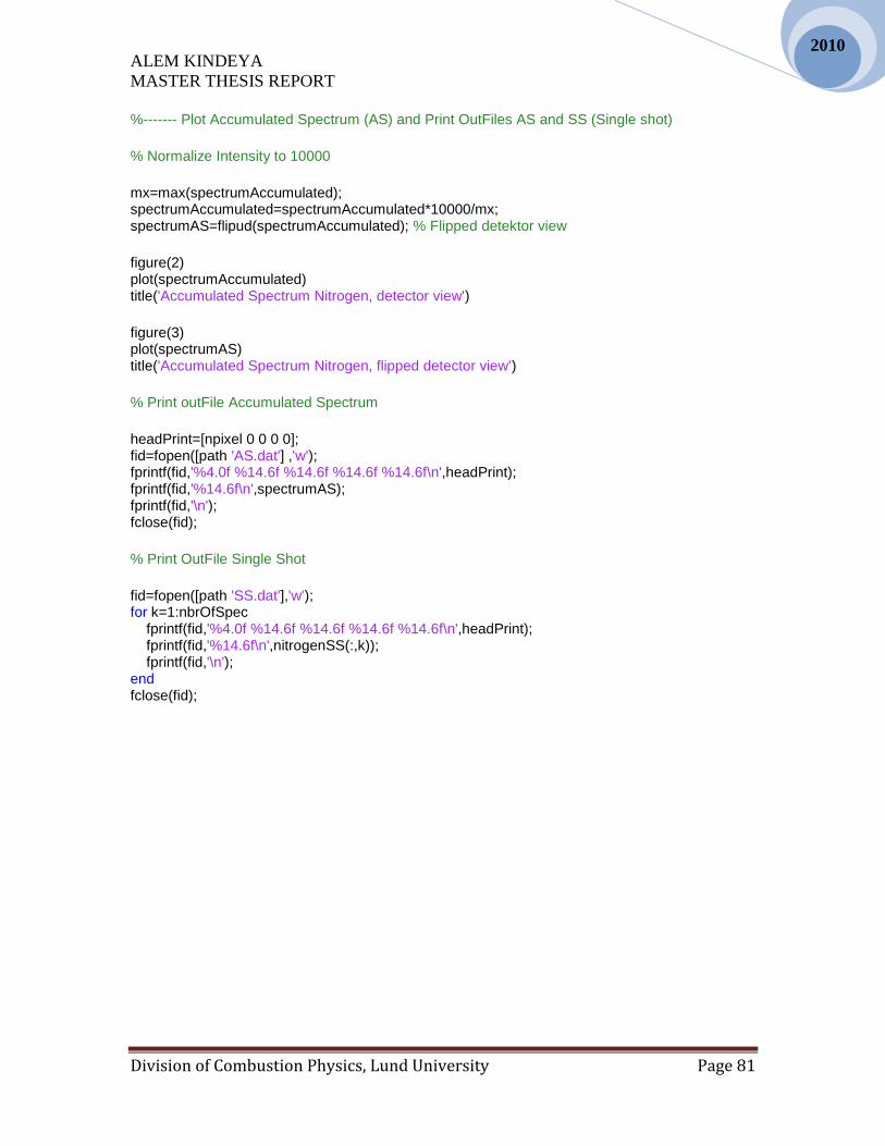
ALEM KINDEYA



2010

%------- Plot Accumulated Spectrum (AS) and Print OutFiles AS and SS (Single shot) % Normalize Intensity to 10000

mx=max(spectrumAccumulated); spectrumAccumulated=spectrumAccumulated*10000/mx; spectrumAS=flipud(spectrumAccumulated); % Flipped detektor view figure(2) plot(spectrumAccumulated) title('Accumulated Spectrum Nitrogen, detector view') figure(3) plot(spectrumAS) title('Accumulated Spectrum Nitrogen, flipped detector view') % Print outFile Accumulated Spectrum

headPrint=[npixel 0 0 0 0]; fid=fopen([path 'AS.dat'] ,'w'); fprintf(fid,'%4.0f %14.6f %14.6f %14.6f %14.6f\n',headPrint); fprintf(fid,'%14.6f\n',spectrumAS); fprintf(fid,'\n'); fclose(fid); % Print OutFile Single Shot

fid=fopen([path 'SS.dat'],'w'); for k=1:nbrOfSpec fprintf(fid,'%4.0f %14.6f %14.6f %14.6f %14.6f\n',headPrint); fprintf(fid,'%14.6f\n',nitrogenSS(:,k)); fprintf(fid,'\n'); end fclose(fid);

ALEM KINDEYA



2010

Appendix A4:

To Calculate the Standard deviation, precision and average SSQ

“CalculatePreStdAvg.m” clear all close all % ---------------Read results of Single-shot------------------ path='C:\Documents and Settings\alemkn\Desktop\Rot.CARS BASIC\Andor Camera\Evaluation\Polyfit\New data\Single shot\N2O\'; [T_VARY SSQ_VARY REF_CH NR] = read_data([path 'evalSS.txt']); amountOfSpectra=500; vecOfSpectra=1:amountOfSpectra; % -----------Mean temperature-----------

meanTemperature=mean(T_VARY); vecOfmeanT=ones(1,amountOfSpectra)*meanTemperature; % Calculate Standard Deviation, Precision and average SSQ

StandardDeviation=std(T_VARY) precision=StandardDeviation/meanTemperature averageSSQ=mean(SSQ_VARY) figure(1) hold on plot(vecOfSpectra,T_VARY,'.') plot(vecOfSpectra,vecOfmeanT,'-') plot(vecOfSpectra,vecOfmeanT+StandardDeviation,'--') plot(vecOfSpectra,vecOfmeanT-StandardDeviation,'--') ylabel('Temperature (K)') xlabel('Number of spectra') legend('Single-shot T','Mean T','StandardDeviation') % -------Plot of SSQ versus temperature-----

figure(2) hold on plot(SSQ_VARY,T_VARY,'.') xlabel('SSQ') ylabel('Temperature (K)') legend('Single-shot SSQ Vs T')

ALEM KINDEYA



2010

Appendix B: Input data file for theoretical library of N2O

Appendix B1:

The N2O.dat file format

Data file N2O.DAT contains spectroscopic constants

and fitted lw-coeficients for N2O

---------------------------------------------------------------------

2358.5849 , 14.33245 , -2.106E-3 , 2.583E-4 ! (1)

0.41901 , 0.172E-6 , 3.449E-3 , -3.0E-6 , 8.320E-9 ! (2)

1.0 , 1.0 ! (3)

1.09768E-8 , 6.91E-25 , 1.4E-16 , 0.0 ! (4)

0.085 , -0.705 , -3.39 , -1.27 , 0.0 , 0.0 ! (5)

---------------------------------------------------------------------

Expl and Refs:

(1) Vibrational constants: Vibrationsfrekvens OMEGAe, Anharmoniska

vibrationskonskonstanter Xe, Ye, Ze;(cm-1)

(2) Rotational constants: Be, De, ALPHAe, GAMMAe, BETAe; (cm-1)

(3) Statistical weights OK!

(4) Rotational-vibrational interaction

(5) Approximation of line widths