1 | P a g e   

Implementation and Simulation of Real‐time Pulse Processing Functions  

Tyler Lutz 28.07.2011 

University of Chicago  

A variety of real‐time pulse analysis procedures, enumerated below, were loaded onto an FPGA for the purpose of extracting relevant information from the raw data generated in photo‐detectors. While 

referencing a few particulars as to how the analysis functions were actually instantiated in the form of VHDL code, this document describes in detail a number of simulations carried out on an FPGA after 

having been programmed with our code. Appendix provides the two raw test pulses used for simulations.  

  

Motivation  

  It is computationally advantageous to perform various data analysis functions on the output signal from a photo‐detector in real time rather than channeling the raw signal to software to perform calculations after the device is finished taking data. Specifically, we would like to know the time of arrival of a given pulse as well as various features of the pulse waveform such as its average height, its full width at half maximum, its rising and falling times, the height of its peak(s), and the number of electrons it represents. Additional data related to the baseline (non‐pulse) signal such as its overall average, its standard deviation, and its significance is also useful for calibrating the actual pulse data.  Approach and Implementation    The real‐time computations will be carried out in an on‐board Field Programmable Gate Array (FPGA), which is fed pulse data in parallel from an ASIC acting as an oscilloscope for the actual photo‐detector. Programmable logic arrays in the FPGA can be manipulated in a number of different ways, and we have chosen to use VHDL code.    We have assumed here that the input data will be passed from the ASIC directly to the FPGA without any mediation in the form of e.g. memory devices, etc. Output readings from the various analysis functions are also in parallel and, at least in the current conception of the code, last for a single clock cycle (the idea is that these quick readings can then be stored somewhere and read later). All output shown in these simulations come directly from the FPGA, an Altera Cyclone IV with serial number EP4CE22F17C6N which was programmed with the appropriate VHDL code using Quartus II software.  

Simulation of Timing Analyses  

Multi‐threshold timing analysis    Perhaps the simplest way to estimate the time of arrival of a pulse is just to record when it crosses certain pre‐determined threshold values. These values are highly dependent on the shape of the pulse, the desired accuracy, and the noise of the background signal, but for the purposes of simulation it suffices to use completely arbitrary thresholds and demonstrate that the program can accurately determine the times of the respective threshold‐crossings. 

2 | P a g e 

Athresholddemonstrof the thr

  

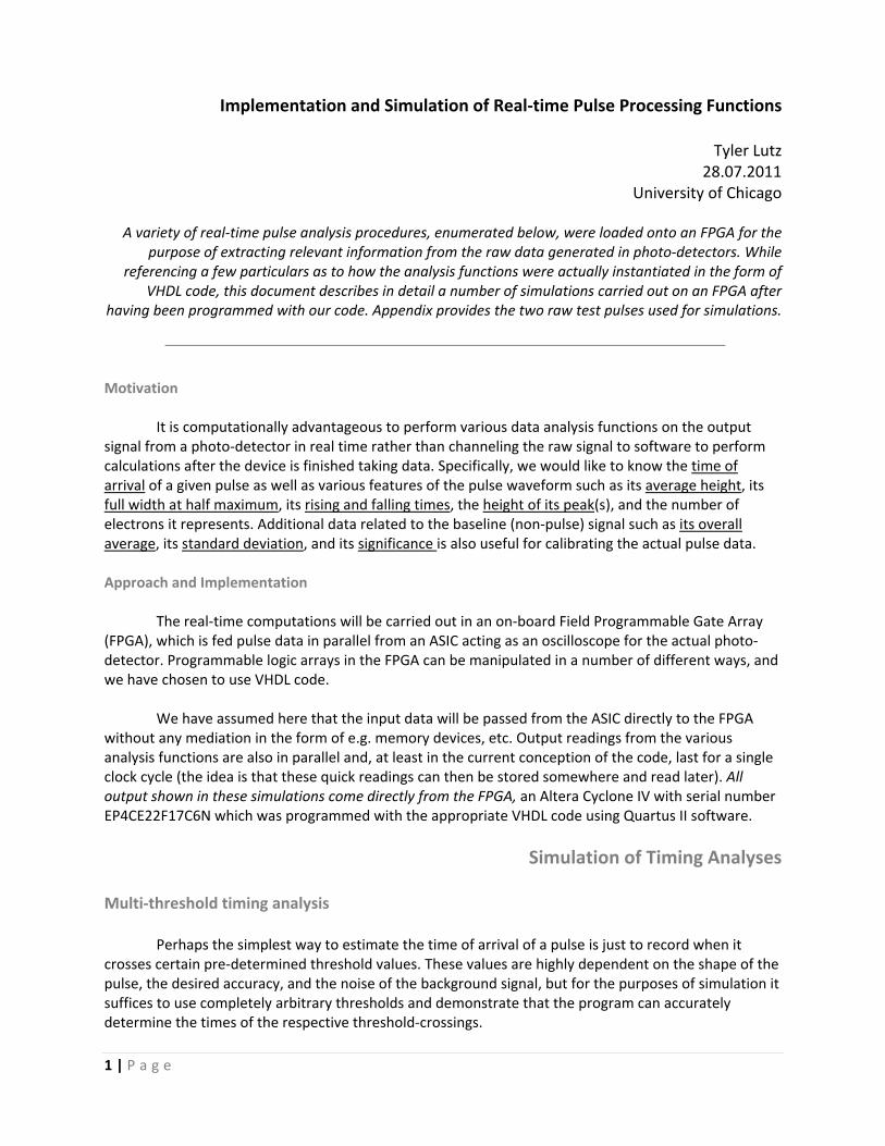
          Fig. 1 : Timfor referen   Thto verify tworking wtimer to vinformatio97µs, so ifabove, we  Ththe same    Ju 

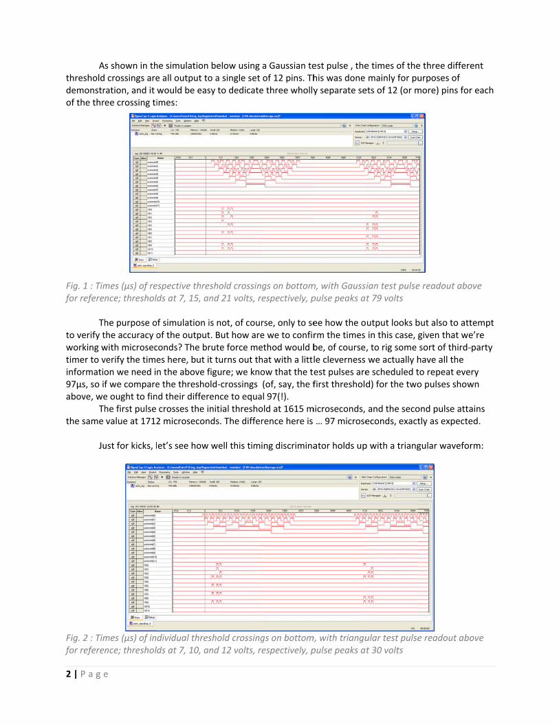
Fig. 2 : Timfor referen

e  

s shown in th crossings areration, and it ee crossing ti

mes (µs) of rence; threshol

he purpose othe accuracy owith microsecverify the timeon we need if we comparee ought to finhe first pulse value at 1712

ust for kicks, l

mes (µs) of innce; threshol

he simulation e all output towould be easimes: 

espective threds at 7, 15, an

f simulation iof the outputconds? The bres here, but in the above fe the threshond their differcrosses the i2 microsecon

et’s see how 

dividual thresds at 7, 10, an

below using o a single set sy to dedicate

eshold crossinnd 21 volts, r

is not, of court. But how arerute force met turns out thfigure; we knoold‐crossings  ence to equanitial threshonds. The differ

well this tim

shold crossingnd 12 volts, r

a Gaussian teof 12 pins. The three wholly

 

gs on bottomespectively, p

rse, only to see we to confirethod would bhat with a littlow that the te(of, say, the fal 97(!). old at 1615 mrence here is 

ing discrimina

gs on bottom,espectively, p

est pulse , thehis was done y separate se

m, with Gausspulse peaks a

ee how the orm the times be, of course,le cleverness est pulses arefirst threshold

microseconds, … 97 microse

ator holds up

m, with triangupulse peaks a

e times of themainly for pu

ets of 12 (or m

ian test pulset 79 volts 

utput looks bin this case, g, to rig some we actually he scheduled td) for the two

and the secoeconds, exact

p with a triang

ular test pulset 30 volts 

e three differeurposes of more) pins for

e readout abo

but also to attgiven that wesort of third‐have all the to repeat eveo pulses show

ond pulse attatly as expecte

gular wavefor

 e readout abo

ent 

r each 

ove 

tempt e’re ‐party 

ry wn 

ains ed. 

rm: 

ove 

3 | P a g e 

  W

     Leading E   Thand then then outp  Thwere it nomitigatedbefore divtruncationsteps of th   A 

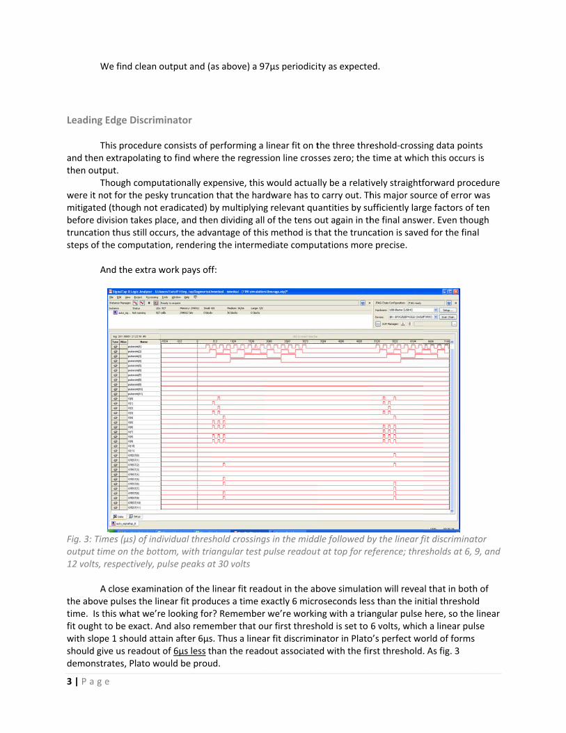
Fig. 3: Timoutput tim12 volts, r   Athe abovetime.  Is thfit ought twith slopeshould givdemonstr

e  

We find clean 

Edge Discrim

his procedureextrapolatingput.  hough compuot for the pes (though not vision takes pn thus still oche computati

nd the extra 

mes (µs) of indme on the botrespectively, p

 close examine pulses the lihis what we’rto be exact. Ae 1 should attve us readoutrates, Plato w

output and (a

minator 

e consists of pg to find wher

utationally exky truncationeradicated) b

place, and thecurs, the advion, rendering

work pays off

dividual thresttom, with triapulse peaks a

nation of the near fit prodre looking forAnd also remetain after 6µst of 6µs less twould be prou

as above) a 9

performing a re the regress

xpensive, this n that the harby multiplyingen dividing allantage of thig the interme

f: 

shold crossingangular test pat 30 volts 

linear fit readuces a time er? Rememberember that ous. Thus a lineahan the readud. 

7µs periodici

linear fit on tsion line cros

would actuardware has tog relevant qu of the tens os method is tediate compu

gs in the middpulse readout

dout in the abexactly 6 micrr we’re workinur first threshar fit discriminout associate

ty as expecte

the three threses zero; the 

lly be a relatio carry out. Thantities by suout again in ththat the truncutations more

dle followed bt at top for re

bove simulatiroseconds lesng with a triahold is set to nator in Platoed with the fir

ed. 

eshold‐crossitime at whic

vely straightfhis major souufficiently larghe final answcation is savee precise. 

by the linear feference; thre

ion will reveas than the iniangular pulse 6 volts, whicho’s perfect worst threshold.

ng data pointh this occurs 

forward proceurce of error wge factors of ter. Even thoud for the fina

 fit discriminatesholds at 6, 9

l that in bothitial thresholdhere, so the h a linear pulsorld of forms . As fig. 3 

ts is 

edure was ten ugh l 

tor 9, and 

h of d linear se 

4 | P a g e 

   Othe same  

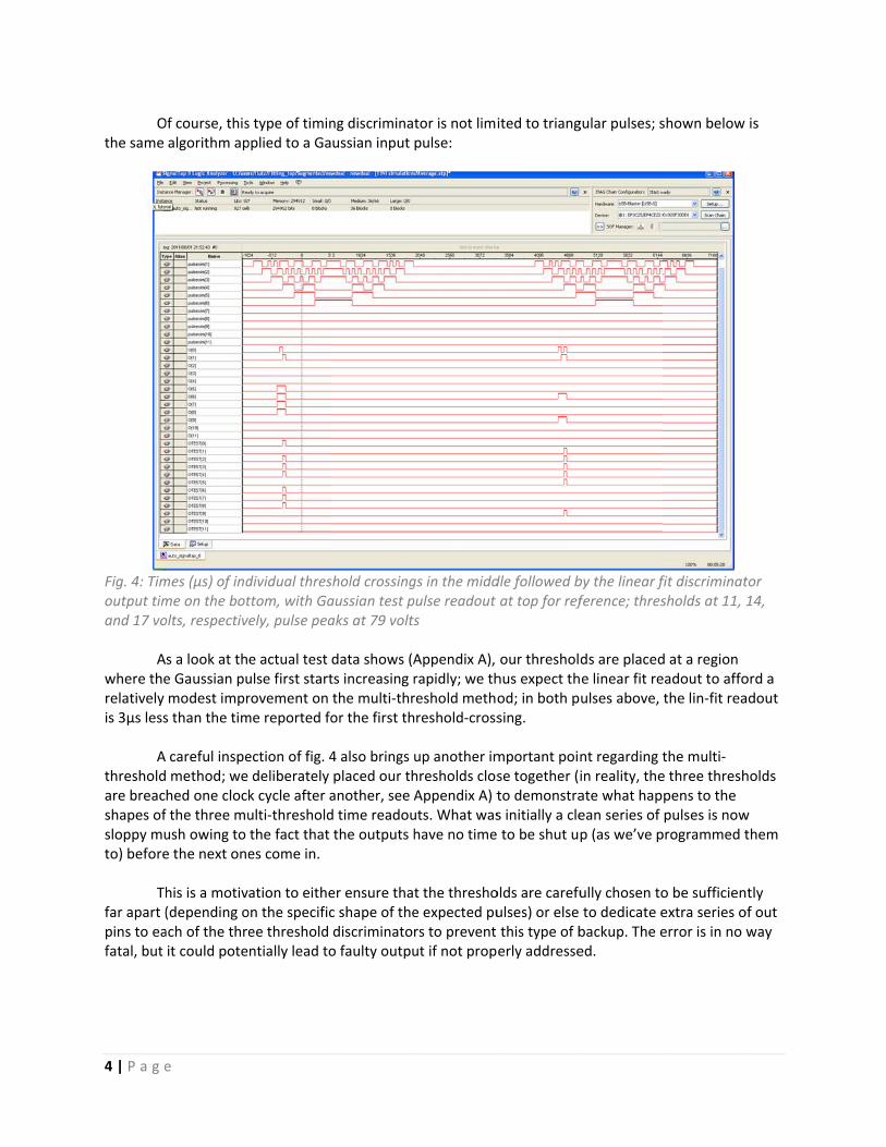
Fig. 4: Timoutput timand 17 vo   Awhere therelatively is 3µs less   Athresholdare breacshapes ofsloppy muto) before 

Thfar apart (pins to eafatal, but     

e  

Of course, thisalgorithm ap

mes (µs) of indme on the botolts, respectiv

s a look at the Gaussian pumodest imprs than the tim

 careful inspe method; we hed one clockf the three muush owing to e the next one

his is a motiv(depending oach of the threit could pote

s type of timinpplied to a Ga

dividual thresttom, with Gaely, pulse pea

e actual test ulse first startrovement on me reported fo

ection of fig. 4deliberately k cycle after aulti‐thresholdthe fact that es come in.  

ation to eitheon the specificee threshold ntially lead to

ng discriminaussian input 

shold crossingaussian test paks at 79 volts

data shows (Ats increasing rthe multi‐thror the first th

4 also brings placed our thanother, see Ad time readouthe outputs h

er ensure thatc shape of thediscriminatoro faulty outpu

tor is not limipulse: 

gs in the middpulse readout s 

Appendix A), rapidly; we threshold methoreshold‐cross

up another imhresholds closAppendix A) tuts. What washave no time

t the threshoe expected purs to prevent ut if not prop

ited to triang

dle followed bat top for ref

our thresholhus expect thod; in both psing. 

mportant poinse together (ito demonstras initially a cle to be shut u

olds are carefuulses) or else this type of berly addresse

gular pulses; s

by the linear fference; thres

ds are placede linear fit reulses above, 

nt regarding tin reality, theate what hapean series of p (as we’ve p

ully chosen toto dedicate ebackup. The eed. 

shown below 

 fit discriminatsholds at 11, 

d at a region eadout to affothe lin‐fit rea

the multi‐e three threshpens to the pulses is nowprogrammed t

o be sufficienextra series oerror is in no 

is 

tor 14, 

ord a adout 

holds 

w them 

tly of out way 

5 | P a g e 

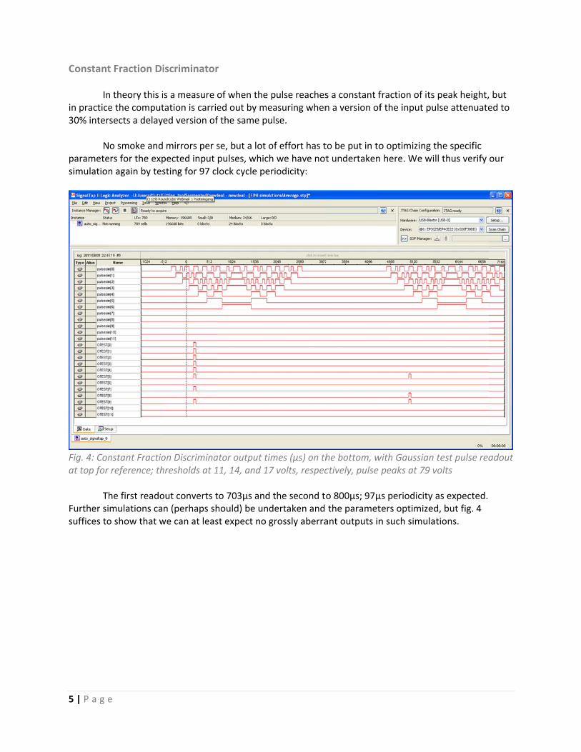
Constant   Inin practice30% inter 

Nparametesimulation

Fig. 4: Conat top for    ThFurther sisuffices to            

e  

t Fraction Di

n theory this ie the computrsects a delay

o smoke anders for the expn again by tes

nstant Fractioreference; th

he first readomulations cao show that w

iscriminator

s a measure otation is carrieed version of

 mirrors per spected input sting for 97 cl

on Discriminahresholds at 1

out converts tn (perhaps shwe can at leas

r 

of when the ped out by mef the same pu

se, but a lot opulses, whichlock cycle per

ator output tim11, 14, and 17

to 703µs and hould) be undst expect no g

pulse reacheseasuring whenulse.  

of effort has th we have notriodicity: 

 

mes (µs) on th7 volts, respec

the second todertaken and grossly aberra

s a constant fn a version of

to be put in tot undertaken

he bottom, wctively, pulse 

o 800µs; 97µthe parametant outputs in

fraction of itsf the input pu

o optimizing t here. We wi

with Gaussian peaks at 79 v

µs periodicity ters optimizedn such simula

 peak height,ulse attenuate

the specific ll thus verify 

test pulse reavolts 

as expected.d, but fig. 4 ations. 

 but ed to 

our 

 adout 

6 | P a g e 

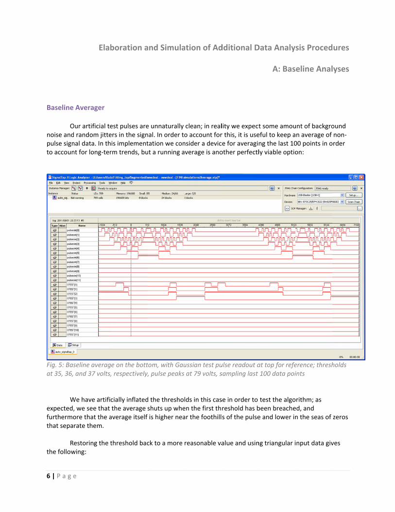
   Baseline    Onoise andpulse signto accoun  

Fig. 5: Basat 35, 36,     Wexpected,furthermothat sepa   Rthe follow 

e  

Elab

Averager 

Our artificial te random jittenal data. In thnt for long‐ter

seline averagand 37 volts,

We have artific, we see that ore that the arate them. 

estoring the twing: 

boration a

est pulses areers in the signis implementrm trends, bu

e on the bott, respectively,

cially inflatedthe average saverage itself 

threshold bac

and Simula

e unnaturally nal. In order totation we conut a running a

tom, with Gau, pulse peaks 

d the thresholshuts up wheis higher nea

ck to a more r

ation of Ad

clean; in realo account fornsider a devicverage is ano

ussian test puat 79 volts, s

lds in this casen the first thar the foothill

reasonable va

dditional D

lity we expectr this, it is usece for averagiother perfectl

ulse readout asampling last 

se in order to reshold has bs of the pulse

alue and usin

Data Analy

A: Bas

t some amoueful to keep ang the last 10ly viable optio

at top for refe100 data poi

test the algobeen breachee and lower in

ng triangular i

sis Proced

eline Anal

unt of backgron average of 00 points in oon: 

erence; threshints 

rithm; as ed, and n the seas of 

nput data giv

ures  

lyses 

ound non‐rder 

holds 

zeros 

ves 

7 | P a g e 

 

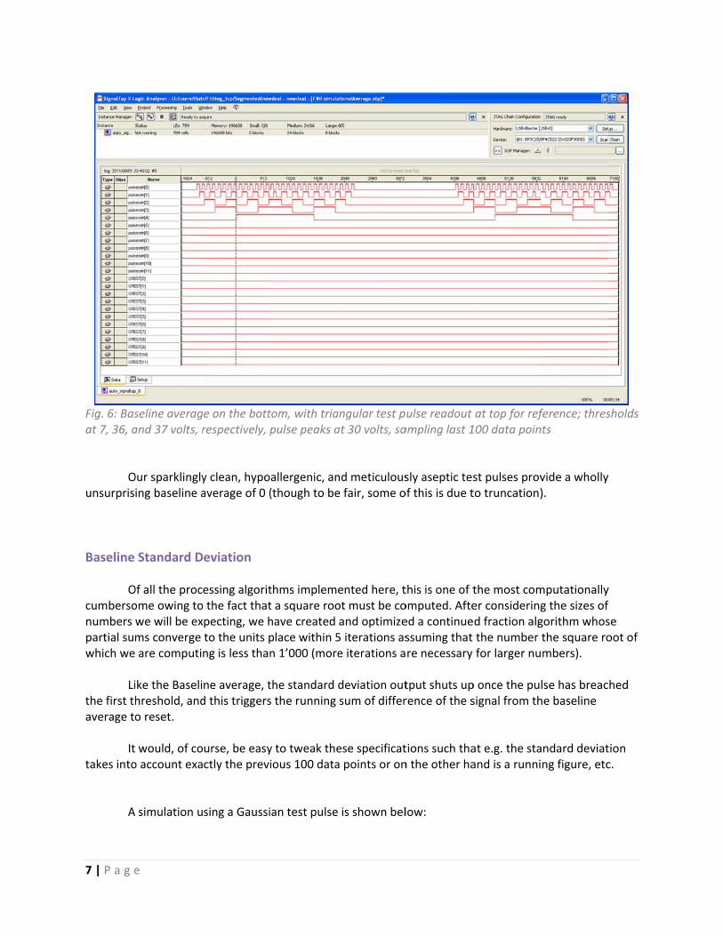
Fig. 6: Basat 7, 36, a   

 O

unsurpris   

Baseline    Ocumbersonumbers partial sumwhich we   Lithe first thaverage to   Ittakes into  

A

  

e  

seline averagand 37 volts, r

Our sparklinglying baseline a

Standard D

Of all the procome owing towe will be exms converge  are computi

ike the Baselihreshold, ando reset. 

 would, of coo account exa

 simulation u

e on the bottrespectively, p

y clean, hypoaverage of 0 (

eviation 

essing algorito the fact thatpecting, we hto the units png is less than

ne average, td this triggers

urse, be easyctly the previ

sing a Gaussi

tom, with triapulse peaks a

allergenic, an(though to be

thms implemet a square roohave created place within 5n 1’000 (more

the standard s the running 

y to tweak theious 100 data

an test pulse

angular test pat 30 volts, sa

nd meticulouse fair, some o

ented here, tot must be coand optimize5 iterations ase iterations a

deviation outsum of differ

ese specificata points or on

 is shown bel

ulse readout ampling last 1

sly aseptic tesof this is due t

this is one of tomputed. Afteed a continuessuming that re necessary 

tput shuts uprence of the s

tions such than the other ha

low: 

at top for ref100 data poin

st pulses provto truncation)

the most comer consideringd fraction algthe number for larger nu

p once the pusignal from th

at e.g. the staand is a runni

ference; thresnts 

vide a wholly). 

mputationallyg the sizes of gorithm whosthe square rombers). 

lse has breache baseline 

andard deviatng figure, etc

 sholds 

 

y 

se oot of 

hed 

tion c.  

8 | P a g e 

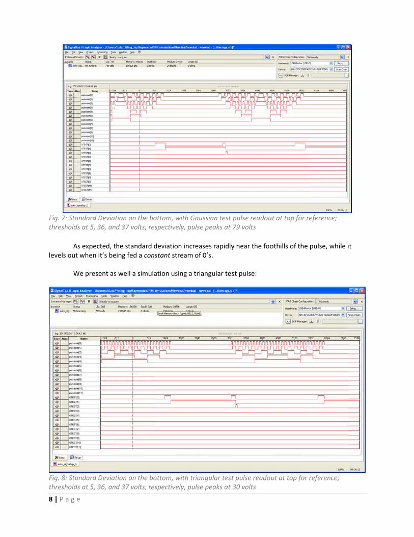
Fig. 7: Stathresholds

   Alevels out   W 

Fig. 8: Stathresholds

e  

andard Deviats at 5, 36, an

s expected, tt when it’s be

We present as

andard Deviats at 5, 36, an

tion on the bod 37 volts, res

he standard ding fed a cons

s well a simula

tion on the bod 37 volts, res

ottom, with Gspectively, pu

deviation incrstant stream 

ation using a 

ottom, with trspectively, pu

Gaussian test ulse peaks at 

reases rapidlyof 0’s. 

triangular tes

riangular testulse peaks at 3

pulse readou79 volts 

y near the foo

st pulse: 

t pulse readou30 volts 

ut at top for re

othills of the 

ut at top for r

eference; 

pulse, while i

reference; 

 

it 

 

9 | P a g e   

                     

  Baseline Significance    (forthcoming)                       

10 | P a g 

 Number    Siit by the c 

  Integral c   Wthe averaactually malgorithm‘time1’ an   A 

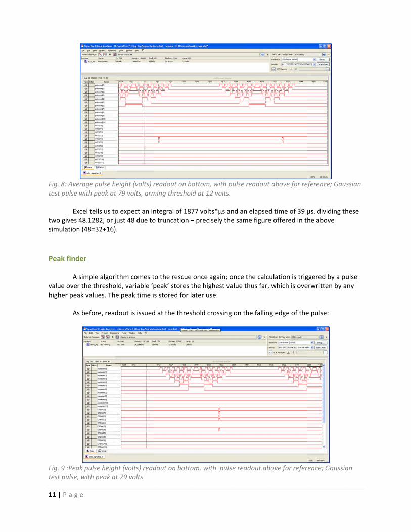
Fig. 7 : Avtriangular    Inspreadshethat timepulse is fiis accurat    Si

g e  

of Electrons

ince this calcucharge of the 

calculator/a

We present thge height calcmean, of courm specifically, nd ‘time2’ res

n illustrative 

verage pulse hr test pulse w

n order to teseet; the total 1 is when therst strictly lese to within tr

imulations we

s 

ulation consiselectron, we

average heig

ese together culator dividese, a simple sthe times of tspectively bot

simulation is 

height (volts) with peak at 30

t this readoutintegral shou

e pulse is greass than the thruncation erro

ere also carrie

sts of nothingwill proceed

ght 

because theyes the integrasum of all of tthe initial andth in the code

shown below

readout on b0 volts, armin

t, we have tauld come out ater than or ereshold againor. 

ed out with a

g more than fdirectly to si

y are effectival calculation the data poind final arminge and for futu

w: 

bottom, with png threshold a

bulated the eto 768 volt*µ

equal to the an). Hence, exp

a Gaussian tes

finding the intmulations of 

vely the same by the elapsets between cg threshold crure reference

pulse readouat 12 volts. 

expected aveµsec, and therming threshpected: 20.75

st pulse, as ill

B: P

tegral of the pthe integral c

 process, saveed time. By ‘incertain boundrossings (whic).  

t above for re

rage value use elapsed timehold while tim567; readout:

lustrated belo

Pulse Anal

pulse and divcalculator: 

e for the factntegral’ here ds—in our ch we’ll label 

 eference; 

sing an Excel e is 37µs (notme2 is when th: 20 (16+4), w

ow: 

lyses 

viding 

 that we 

te he which 

11 | P a g 

Fig. 8: Avetest pulse   Extwo gives simulation

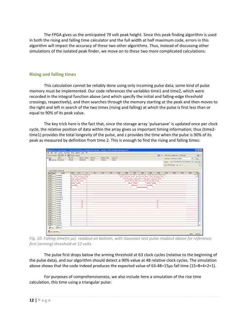
  Peak find   Avalue ovehigher pe     A 

Fig. 9 :Peatest pulse,

g e  

erage pulse he with peak at

xcel tells us to48.1282, or jn (48=32+16)

der 

 simple algorr the threshoak values. Th

s before, read

ak pulse heighe, with peak a

height (volts) rt 79 volts, arm

o expect an injust 48 due to). 

ithm comes told, variable ‘pe peak time i

dout is issued

ht (volts) readt 79 volts 

readout on boming threshol

ntegral of 187o truncation –

to the rescue peak’ stores ts stored for la

d at the thres

dout on botto

ottom, with pld at 12 volts.

77 volts*µs a– precisely th

once again; othe highest vaater use.  

hold crossing

om, with  puls

pulse readout 

nd an elapsede same figure

once the calcalue thus far,

g on the fallin

se readout ab

t above for ref

d time of 39 µe offered in th

ulation is trig which is ove

g edge of the

bove for refer

 ference; Gaus

µs. dividing thhe above 

ggered by a puerwritten by a

e pulse: 

 rence; Gaussia

ssian 

hese 

ulse any 

an 

12 | P a g 

   Thin both thalgorithmsimulation   

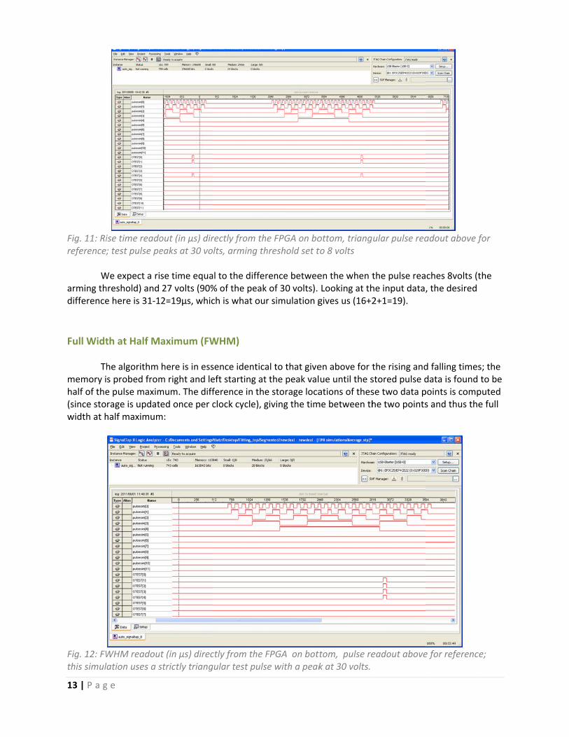
  Rising an   Thmemory mrecorded crossings,the right aequal to 9   Thcycle, thetime1) propeak as m 

Fig. 10: Fafirst (armi   Ththe pulse above sho

 Fo

calculatio  

g e  

he FPGA givehe rising and fm will impact tns of the isola

nd falling tim

his calculatiomust be implein the integra, respectivelyand left in sea90% of its pea

he key trick h relative posiovides the tomeasured by d

alling time(in ing) threshold

he pulse first data), and ouows that the c

or purposes on, this time u

s us the anticfalling time cathe accuracy oated peak find

mes 

n cannot be remented. Oual function ab), and then search of the twak value.  

here is the faction of data wtal longevity definition from

µs)  readout d at 12 volts 

drops belowur algorithm scode indeed 

of comprehenusing a triangu

cipated 79 voalculator and of these two der, we move

reliably done r code referebove (and whearches throuwo times (risin

ct that, since twithin the arrof the pulse, m time 2. Thi

on bottom, w

 the arming tshould detectproduces the

nsiveness, weular pulse: 

lt peak heighthe full widthother algorite on to these 

using only inences the variich specify thugh the memng and falling

the storage aray gives us imand z provides is enough to

with Gaussian

threshold at 6t a 90% valuee expected va

e also include 

t. Since this ph at half maxhms. Thus, intwo more co

coming pulseiables time1 ahe initial and fory starting ag) at which th

array ‘pulsarsamportant times the time wo find the risi

n test pulse re

63 clock cyclee at 48 relativlue of 63‐48=

here a simul

peak finding aimum code, enstead of discomplicated ca

e data; some and time2, wfalling‐edge tat the peak ane pulse is firs

ave’ is updateing informatiwhen the pulsing and falling

eadout above

es (relative to ve clock cycles=15µs fall tim

ation of the r

algorithm is uerrors in this ussing other alculations: 

kind of pulse hich were threshold nd then movest less than or

ed once per con; thus (timse is 90% of itg times: 

  for reference

the beginnins. The simulate (15=8+4+2+

rise time 

used 

es to r 

clock e2‐ts 

e; 

ng of tion +1). 

13 | P a g 

 

     

        Fig. 11: Rireference;   Warming thdifference

  Full Widt

 Th

memory ihalf of the(since stowidth at h 

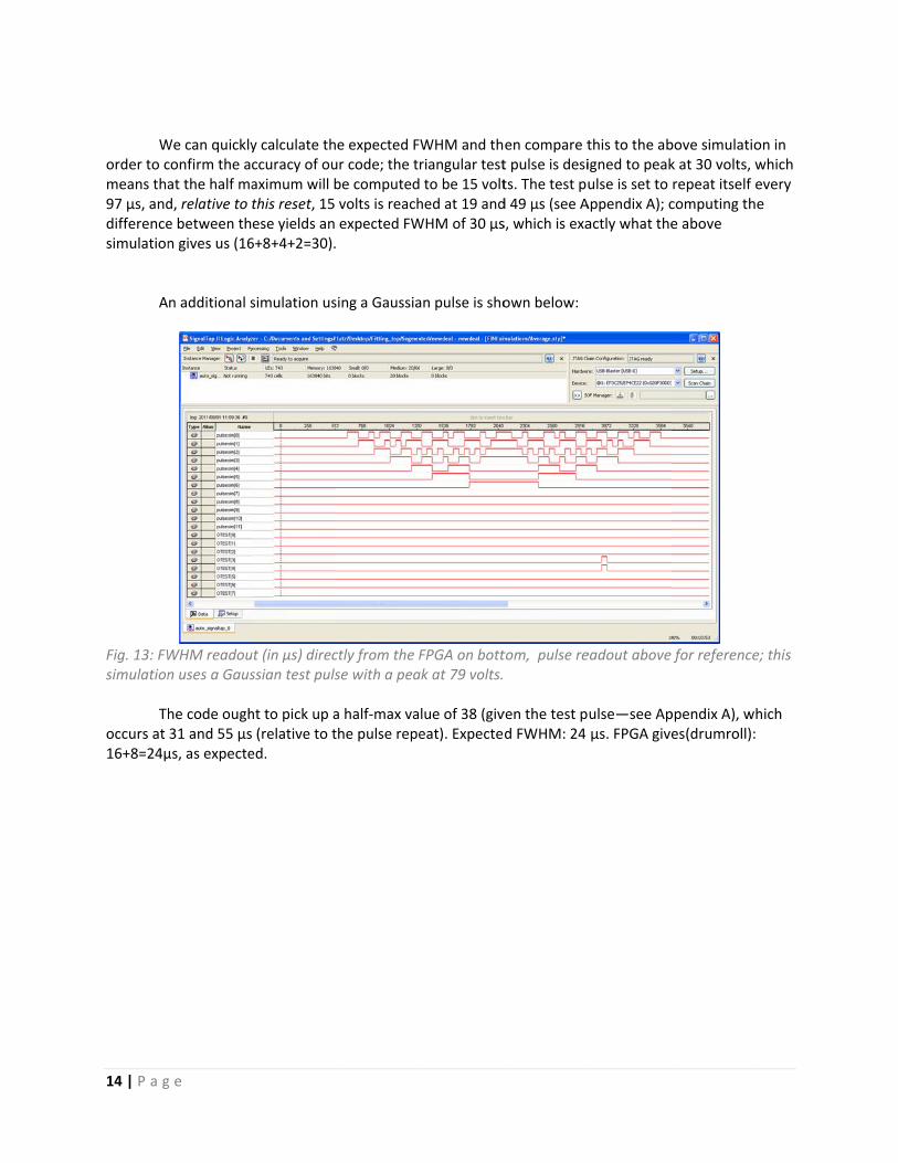
Fig. 12: FWthis simul

g e  

ise time reado; test pulse pe

We expect a rihreshold) and e here is 31‐1

th at Half M

he algorithm s probed frome pulse maximrage is updathalf maximum

WHM readoulation uses a s

out (in µs) direaks at 30 vo

se time equa27 volts (90%

12=19µs, whic

aximum (FW

here is in essm right and lemum. The diffted once per cm: 

ut (in µs) direcstrictly triang

rectly from thlts, arming th

al to the differ% of the peakch is what ou

WHM) 

sence identicaeft starting atference in theclock cycle), g

ctly from the Fgular test puls

 

e FPGA on bohreshold set t

rence betweek of 30 volts). r simulation g

al to that givet the peak vale storage locagiving the tim

FPGA  on bottse with a peak

ottom, triangto 8 volts 

en the when tLooking at thgives us (16+2

en above for tue until the sations of thesme between th

tom,  pulse rek at 30 volts.

ular pulse rea

the pulse reahe input data,2+1=19). 

the rising andstored pulse dse two data phe two points

eadout above

adout above f

ches 8volts (t, the desired 

d falling timesdata is found points is comps and thus the

 e for reference

for 

the 

s; the to be puted e full 

e; 

14 | P a g 

    Worder to cmeans tha97 µs, anddifferencesimulation

  A 

Fig. 13: FWsimulation   Thoccurs at 16+8=24µ               

g e  

We can quicklyconfirm the aat the half mad, relative to e between thn gives us (16

n additional s

WHM readoun uses a Gaus

he code ough31 and 55 µsµs, as expecte

y calculate thccuracy of ouaximum will bthis reset, 15 ese yields an 6+8+4+2=30).

simulation us

ut (in µs) direcssian test puls

ht to pick up a (relative to ted. 

e expected Fur code; the trbe computedvolts is reachexpected FW 

sing a Gaussia

ctly from the Fse with a pea

a half‐max vathe pulse repe

WHM and thriangular test to be 15 volthed at 19 andWHM of 30 µs

an pulse is sho

FPGA on bottak at 79 volts.

lue of 38 (giveat). Expecte

en compare tt pulse is desits. The test pud 49 µs (see As, which is exa

own below:

tom,  pulse re 

ven the test pd FWHM: 24 

this to the abigned to peakulse is set to Appendix A); cactly what the

eadout above 

ulse—see Apµs. FPGA give

bove simulatiok at 30 volts, wrepeat itself ecomputing the above 

 for reference

ppendix A), whes(drumroll):

on in which every e 

e; this 

hich  

15 | P a g e   

Appendix A: Test‐pulse data Triangular pulse:       Clock cycle          Signal 

0  :  0 

1  :  0 

2  :  0 

3  :  0 

4  :  0 

5  :  1 

6  :  2 

7  :  3 

8  :  4 

9  :  5 

10  :  6 

11  :  7 

12  :  8 

13  :  9 

14  :  10 

15  :  11 

16  :  12 

17  :  13 

18  :  14 

19  :  15 

20  :  16 

21  :  17 

22  :  18 

23  :  19 

24  :  20 

25  :  21 

26  :  22 

27  :  23 

28  :  24 

29  :  25 

30  :  26 

31  :  27 

32  :  28 

     

     

     

     

     

     

     

     

33  :  29 

34  :  30 

35  :  29 

36  :  28 

37  :  27 

38  :  26 

39  :  25 

40  :  24 

41  :  23 

42  :  22 

43  :  21 

44  :  20 

45  :  19 

46  :  18 

47  :  17 

48  :  16 

49  :  15 

50  :  14 

51  :  13 

52  :  12 

53  :  11 

54  :  10 

55  :  9 

56  :  8 

57  :  7 

58  :  6 

59  :  5 

60  :  4 

61  :  3 

62  :  2 

63  :  1 

64  :  0  …This is followed by 32 points of insignificant data (0’s), after which the pulse repeats starting at cycle 0 above. 

  

   

16 | P a g e   

Gaussian:  

   Clock cycle                   Signal 

0  :  0 

1  :  0 

2  :  0 

3  :  0 

4  :  0 

5  :  0 

6  :  0 

7  :  0 

8  :  0 

9  :  0 

10  :  0 

11  :  0 

12  :  0 

13  :  0 

14  :  1 

15  :  1 

16  :  2 

17  :  2 

18  :  3 

19  :  4 

20  :  5 

21  :  7 

22  :  8 

23  :  10 

24  :  13 

25  :  15 

26  :  18 

27  :  22 

28  :  25 

29  :  29 

30  :  34 

31  :  38 

32  :  43 

33  :  48 

34  :  53 

35  :  57 

36  :  62 

37  :  66 

38  :  70 

39  :  73 

40  :  76 

41  :  78 

42  :  79 

43  :  79 

44  :  79 

45  :  78 

46  :  76 

47  :  73 

48  :  70 

49  :  66 

50  :  62 

51  :  57 

52  :  53 

53  :  48 

54  :  43 

55  :  38 

56  :  34 

57  :  29 

58  :  25 

59  :  22 

60  :  18 

61  :  15 

62  :  13 

63  :  10 

64  :  8 

65  :  7 

66  :  5 

67  :  4 

68  :  3 

69  :  2 

70  :  2 

71  :  1 

72  :  1 

73  :  0 

74  :  0 

75  :  0 

76  :  0  … followed by 20 points of insignificant data (0’s), after which the pulse repeats starting at cycle 0 above.