implementation and comparative study of image fusion algorithms

International Journal of Computer Applications (0975 – 8887)

Volume 9– No.2, November 2010

25

Implementation and Comparative Study of Image Fusion

Algorithms

Shivsubramani Krishnamoorthy

Centre for Excellence in Computational

Engineering,

Amrita University, Coimbatore, India.

K P Soman Centre for Excellence in Computational

Engineering,

Amrita University, Coimbatore, India.

ABSTRACT Image Fusion is a process of combining the relevant

information from a set of images, into a single image, wherein

the resultant fused image will be more informative and

complete than any of the input images. This paper discusses

the implementation of three categories of image fusion

algorithms – the basic fusion algorithms, the pyramid based

algorithms and the basic DWT algorithms, developed as an

Image Fusion Toolkit - ImFus, using Visual C++ 6.0. The

objective of the paper is to assess the wide range of algorithms

together, which is not found in the literature. The fused

images were assessed using Structural Similarity Image

Metric (SSIM) [10], Laplacian Mean Squared Error along

with seven other simple image quality metrics that helped us

measure the various image features; which were also

implemented as part of the toolkit. The readings produced by

the image quality metrics, based on the image quality of the

fused images, were used to assess the algorithms. We used

Pareto Optimization method to figure out the algorithm that

consistently had the image quality metrics produce the best

readings. An assessment of the quality of the fused images

was additionally performed with the help of ten respondents

based on their visual perception, to verify the results produced

by the metric based assessment. Coincidentally, both the

assessment methods matched in their raking of the algorithms.

The Pareto Optimization method picked DWT with Haar

fusion method as the one with the best image quality metrics

readings. The result here was substantiated by the visual

perception based method where it was inferred that fused

images produced by DWT with Haar fusion method was

marked the best 63.33% of times which was far better than

any other algorithm. Both the methods also matched in

assessing Morphological Pyramid method as producing fused

images of inferior quality.

Keywords Image Fusion, Principal Component Analysis, Pyramid

Methods, Discrete Wavelet Transform, Image Quality

Metrics, Pareto Optimality.

1. INTRODUCTION Any piece of information makes sense only when it is able to

convey the content across. The clarity of information is

important. Image Fusion is a mechanism to improve the

quality of information from a set of images. By the process of

image fusion the good information from each of the given

images is fused together to form a resultant image whose

quality is superior to any of the input images.

This is achieved by applying a sequence of operators on the

images that would make the good information in each of the

image prominent. The resultant image is formed by combining

such magnified information from the input images into a

single image.

1.1 Evolution of fusion techniques The evolution of the research work into the field of image

fusion [9] [17] [24] [25] [26] can be broadly put into the

following three stages

Simple Image Fusion

Pyramid Decomposition based fusion

Discrete Wavelet transform based fusion

The eleven algorithms implemented and discussed here are

such that all the three of the above categories are covered for

assessment.

The primitive fusion schemes [9] perform the fusion right on

the source images. This would include operations like

averaging, addition, subtraction/omission of the pixel

intensities of the input images to be fused. These methods

often have serious side effects such as reducing the contrast of

the image as a whole. But these methods do prove good for

certain particular cases wherein the input images have an

overall high brightness and high contrast. The primitive fusion

methods considered were

Averaging Method

Select Maximum

Select Minimum

With the introduction of pyramid transform [2] [3] [4] [5] [6]

[9] in mid-80's, some sophisticated approaches began to

emerge. People found that it would be better to perform the

fusion in the transform domain. Pyramid transform appears to

be very useful for this purpose. The basic idea is to construct

the pyramid transform of the fused image from the pyramid

transforms of the source images, and then the fused image is

obtained by taking inverse pyramid transform. Pyramid

transform could provide information on the sharp contrast

changes, to which the human visual system is peticularly

sensitive to and It could also provide both spatial and

frequency domain localization. The pyramid fusion methods

considered here were

1 Shivsubramani Krishnamoorthy is currently a PhD student at

MIND Lab, University of Maryland, College Park, MD

20742, USA.



26

Laplacian Pyramid

Ratio-of-low-pass Pyramid

Gradient Pyramid

FSD Pyramid

Morphological Pyramid etc.

Wavelet transforms [2] [6] [7] [9] [12] [16] [24] can be taken

as a special type of pyramid decompositions. It retains most of

the advantages for image fusion but has much more complete

theoretical support. The couple of wavelet transform methods

considered here are

Haar Wavelet transform method

Daubechies (2, 2) wavelet transform method.

1.2 Objective The main objective of this paper is to

Provide a study of 11 pixel based image fusion

techniques.

Discuss some of the implementation issues for the

same.

Assess the algorithms with 9 image quality metrics.

Also assess the algorithms in terms of visual

perception, with the help of 10 respondents and

compare it with the assessment made with the

metrics.

We did not find in the literature a paper that

encompasses such a wide range of image fusion

methods. This paper aims in presenting these

methods in a simplified manner, concentrating more

on the implementation aspects of the algorithms.

We employed Pareto Optimization method [32] to pick out the

algorithm for which the quality metrics consistently produced

the best readings. The methods projected DWT with Haar

based fusion method as superior based on the image quality

metric readings. The same was validated by the assessment

performed based on visual perception which also saw DWT

with Haar based fusion method being selected as the best

63.33% times; which was way more that the other fusion

methods. Both the assessment technique also assessed

Morphological Pyramid based Fusion method as the inferior

methods of the eleven algorithms considered.

2. IMAGE FUSION ALGORITHMS In this section we discuss the set of image fusion algorithms

we considered, categorizing them under three subsections

2.1 Simple Fusion Algorithms The trivial image fusion techniques mainly perform a very

basic operation like pixel selection, addition, subtraction or

averaging. These methods are not always effective but are at

times critical based on the kind of image under consideration.

The trivial image fusion techniques studied and developed as

part of the project are

2.1.1 Average Method Here, the resultant image is obtained by averaging every

corresponding pixel in the input images.

2.1.2 Select Maximum/Minimum Method A selection process if performed here wherein, for every

corresponding pixels in the input images, the pixel with

maximum/minimum intensity is selected, respectively, and is

put in as the resultant pixel of the fused image.

2.1.3 Principal Component Analysis Algorithm

Principal component analysis (PCA) [29] [30] is a vector

space transform often used to reduce multidimensional data

sets to lower dimensions for analysis. It reveals the internal

structure of data in an unbiased way. We provide below the

stepwise description of how we used the PCA algorithm for

fusion.

1. Generate the column vectors, respectively, from the

input image matrices.

2. Calculate the covariance matrix of the two column

vectors formed in 1

3. The diagonal elements of the 2x2 covariance vector

would contain the variance of each column vector

with itself, respectively.

4. Calculate the Eigen values and the Eigen vectors of

the covariance matrix

5. Normalize the column vector corresponding to the

larger Eigen value by dividing each element with

mean of the Eigen vector.

6. The values of the normalized Eigen vector act as the

weight values which are respectively multiplied

with each pixel of the input images.

7. Sum of the two scaled matrices calculated in 6 will

be the fused image matrix.

2.2 Pyramid Fusion Algorithm The decade of 1980’s saw the introduction of pyramid

transform [2] [3] [4] [5] [6] [9] - a fusion method in the

transform domain. An image pyramid [17] consists of a set of

low pass or bandpass copies of an image, each copy

representing pattern information of a different scale. At every

level of fusion using pyramid transform, the pyramid would

be half the size of the pyramid in the preceding level and the

higher levels will concentrate upon the lower spatial

frequencies. The basic idea is to construct the pyramid

transform of the fused image from the pyramid transforms of

the source images and then the fused image is obtained by

taking inverse pyramid transform.

Typically, every pyramid transform consists of three major

phases:

Decomposition

Formation of the initial image for recomposition.

Recomposition

Decomposition is the process where a pyramid is generated

successively at each level of the fusion. The depth of fusion or

number of levels of fusion is pre decided. Decomposition

phase basically consists of the following steps. These steps are

performed l number of times, l being the number of levels to

which the fusion will be performed.

Low Pass filtering. The different pyramidal methods

have a pre defined filter with which are the input

images convolved/filtered with.

Formation of the pyramid for the level from the

filtered/convolved input images using Burt’s

method or Lis Method.

The input images are decimated to half their size,

which would act as the input image matrices for the

next level of decomposition.

Merging the input images is performed after the

decomposition process. This resultant image matrix would act

as the initial input to the recomposition process. The finally



27

decimated input pair of images is worked upon either by

averaging the two decimated input images, selecting the first

decimated input image or selecting the second decimated

input image.

The recomposition is the process wherein, the resultant image

is finally developed from the pyramids formed at each level of

decomposition. The various steps involved in the

recomposition phase are discussed below. These steps are

performed l number of times as in the decomposition process.

The input image to the level of recomposition is

undecimated

The undecimated matrix is convolved/filtered with

the transpose of the filter vector used in the

decomposition process

The filtered matrix is then merged, by the process of

pixel intensity value addition, with the pyramid

formed at the respective level of decomposition.

The newly formed image matrix would act as the

input to the next level of recomposition.

The merged image at the final level of

recomposition will be the resultant fused image. The

flow of the pyramid based image fusion can be

explained by the following example.

Each of the pyramidal algorithms considered by us differ in

the way the decomposition is performed. The Recomposition

phase also differs accordingly. We discuss the pyramid

algorithms we implemented below.

2.2.1 Filter Subtract Decimate Pyramid As suggested by the very name of this algorithm, the

decomposition phase consists of three steps:

Low pass filtering using W = [1

16,

4

16,

6

16,

4

16,

1

16].

Subtract the low pass filtered input images and form

the pyramid

Decimate the input image matrices by halving the

number of rows and columns (we did by neglecting

every alternate row and column).

The recomposition phase would include steps:

Undecimating the image matrix by duplicating

every row and column

Low pass filtering with 2*W

Matrix addition of the same with the pyramid

formed in the corresponding level

2.2.2 Laplacian Pyramid The Laplacian pyramidal method is identical to FSD pyramid

except for an additional low pass filtering performed with

2*W. All the other steps are followed as in FSD pyramid.

2.2.3 Ratio Pyramid The Ration pyramidal method is also identical to FSD

pyramid except for, in the decomposition phase, after low pass

filtering the input image matrices, the pixel wise ratio is

calculated instead of subtraction as in FSD.

2.2.4 Gradient Pyramid The decomposition process here would include the following

steps:

Two low pass filters are considered here W =

[1

16,

4

16,

6

16,

4

16,

1

16] and V = [

1

4,

2

4,

1

4].

Additional to this, four directional filters are applied

on to the input image matrices.

o Horizontal filter 0 0 01 −2 10 0 0

o Vertical filter 0 1 00 −2 00 1 0

o Diagonal filter 0 0 0.50 −1 0

0.5 0 0

o Diagonal filter 0.5 0 00 −1 00 0 0.5

The rest of the steps are similar to that of FSD

pyramid method.

2.2.5 Morphological Pyramid The decomposition phase in this method consists of the

following steps:

Two levels of filtering are performed on the input

image matrices – image opening and image closing.

Image opening is a combination of image erosion

followed by image dilation. Image closing is the

other way round. A combination of image opening

and image closing gets rid of noise in the image[31].

The rest of the steps are as in FSD pyramid method

The recomposition phase would be similar to the FSD method

except for the step where the low pass filter is applied on the

image matrix. Instead, an image dilation is performed over the

matrix.

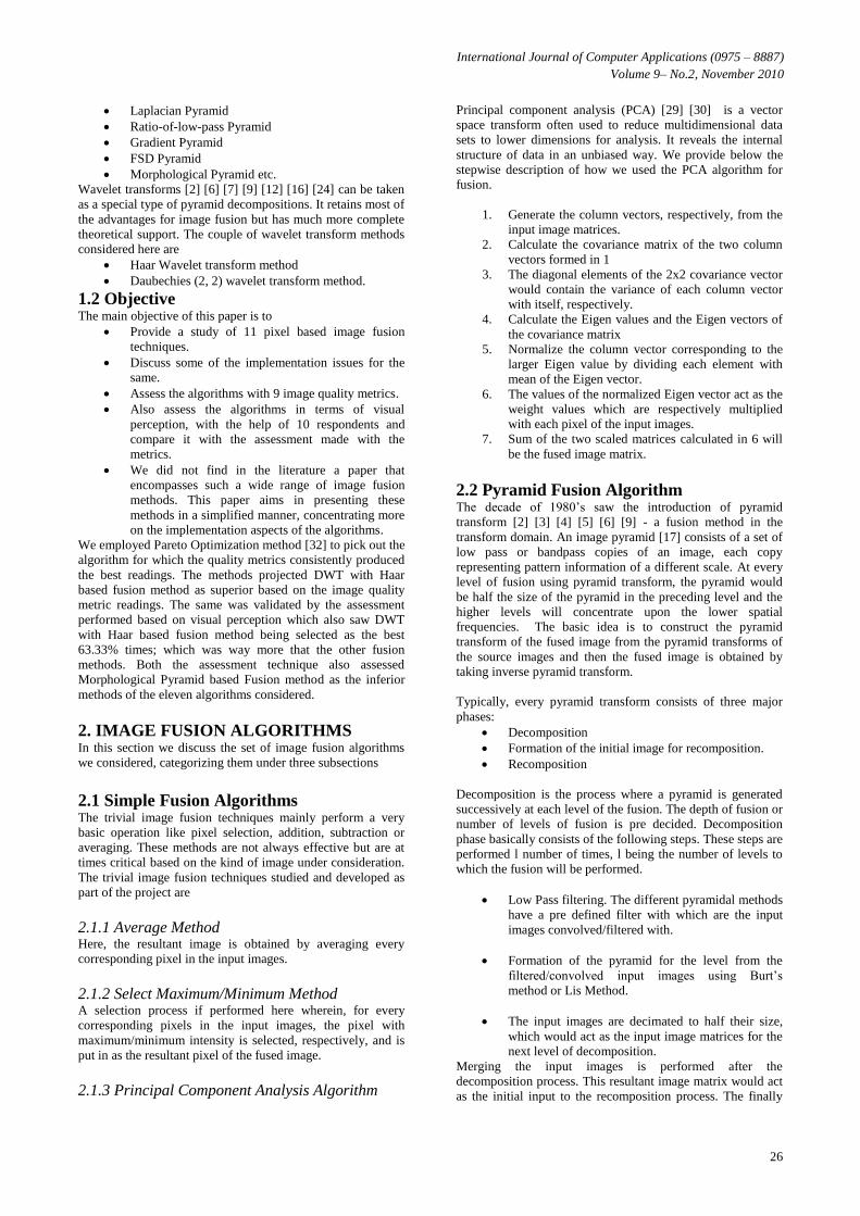
2.3 Discrete Wavelet Transform Method DWT[2][6][7][9][12][16][24] captures not only a notion of

frequency content of the input, by examining it at different

scales, but also temporal content; i.e. the times at which these

frequencies occur. The DWT of a signal x is calculated by

passing it through a series of filters . First the passing it

through a series of filters. First the samples are passed through

a low pass filter with impulse response g resoluting in a

convolution of the two:

( )k

y n x g n x k g n k

The signal is also decomposed simultaneously using a high-

pass filter h. The outputs give the detail coefficients (from the

high-pass filter) and approximation coefficients (from the

low-pass).

This decomposition is repeated to further increase the

frequency resolution and the approximation coefficients

decomposed with high and low pass filters and then down

sampled. This is represented as a binary tree with nodes

representing a sub-space with different time-frequency

localization. The tree is known as a filter bank.

http://en.wikipedia.org/wiki/Image:Wavelets_-_DWT.png



28

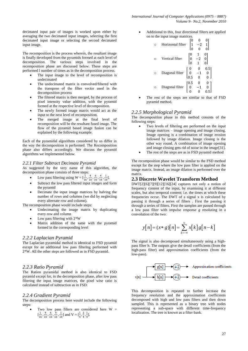
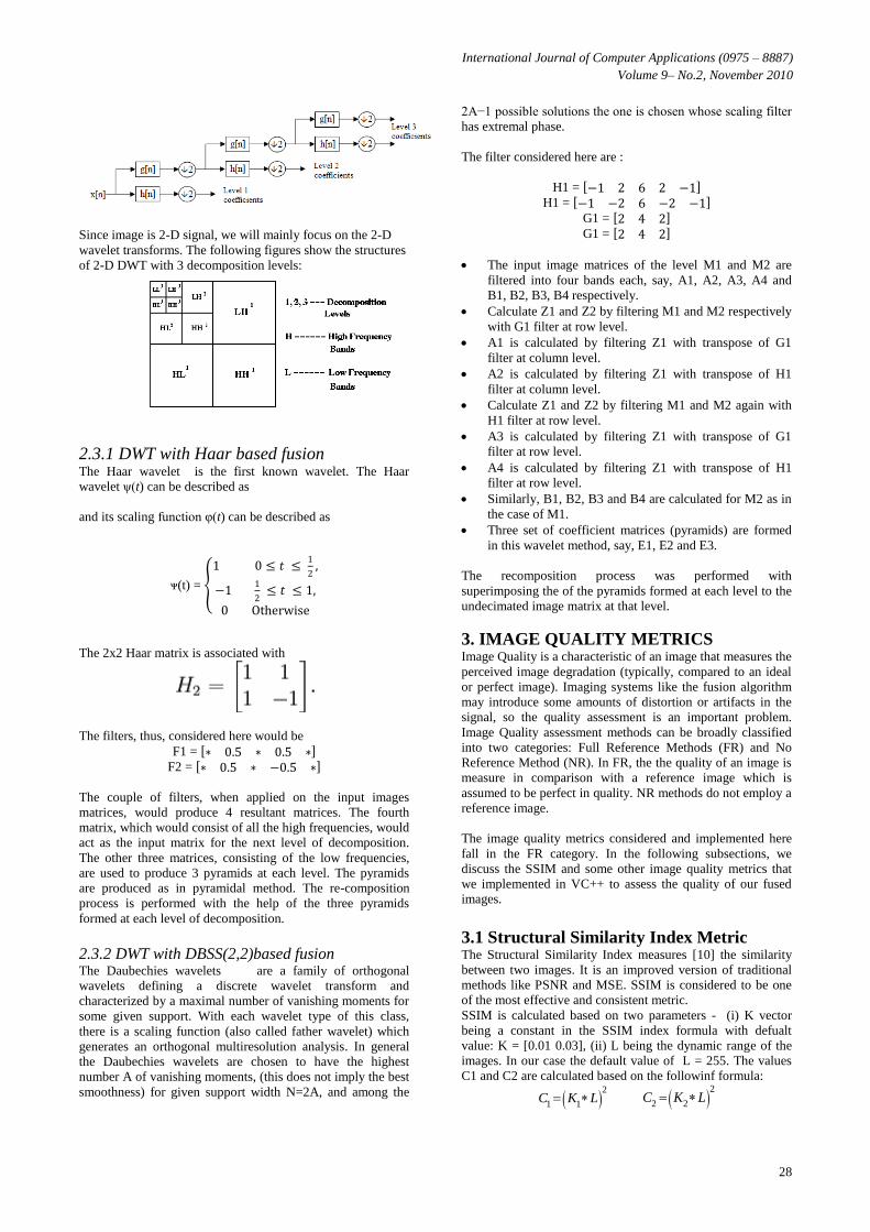
Since image is 2-D signal, we will mainly focus on the 2-D

wavelet transforms. The following figures show the structures

of 2-D DWT with 3 decomposition levels:

2.3.1 DWT with Haar based fusion The Haar wavelet is the first known wavelet. The Haar

wavelet ψ(t) can be described as

and its scaling function φ(t) can be described as

ᴪ(t) =

1 0 ≤ 𝑡 ≤ 1

2,

−1 1

2 ≤ 𝑡 ≤ 1,

0 Otherwise

The 2x2 Haar matrix is associated with

The filters, thus, considered here would be

F1 = ∗ 0.5 ∗ 0.5 ∗ F2 = ∗ 0.5 ∗ −0.5 ∗

The couple of filters, when applied on the input images

matrices, would produce 4 resultant matrices. The fourth

matrix, which would consist of all the high frequencies, would

act as the input matrix for the next level of decomposition.

The other three matrices, consisting of the low frequencies,

are used to produce 3 pyramids at each level. The pyramids

are produced as in pyramidal method. The re-composition

process is performed with the help of the three pyramids

formed at each level of decomposition.

2.3.2 DWT with DBSS(2,2)based fusion The Daubechies wavelets are a family of orthogonal

wavelets defining a discrete wavelet transform and

characterized by a maximal number of vanishing moments for

some given support. With each wavelet type of this class,

there is a scaling function (also called father wavelet) which

generates an orthogonal multiresolution analysis. In general

the Daubechies wavelets are chosen to have the highest

number A of vanishing moments, (this does not imply the best

smoothness) for given support width N=2A, and among the

2A−1 possible solutions the one is chosen whose scaling filter

has extremal phase.

The filter considered here are :

H1 = −1 2 6 2 −1 H1 = −1 −2 6 −2 −1

G1 = 2 4 2 G1 = 2 4 2

The input image matrices of the level M1 and M2 are

filtered into four bands each, say, A1, A2, A3, A4 and

B1, B2, B3, B4 respectively.

Calculate Z1 and Z2 by filtering M1 and M2 respectively

with G1 filter at row level.

A1 is calculated by filtering Z1 with transpose of G1

filter at column level.

A2 is calculated by filtering Z1 with transpose of H1

filter at column level.

Calculate Z1 and Z2 by filtering M1 and M2 again with

H1 filter at row level.

A3 is calculated by filtering Z1 with transpose of G1

filter at row level.

A4 is calculated by filtering Z1 with transpose of H1

filter at row level.

Similarly, B1, B2, B3 and B4 are calculated for M2 as in

the case of M1.

Three set of coefficient matrices (pyramids) are formed

in this wavelet method, say, E1, E2 and E3.

The recomposition process was performed with

superimposing the of the pyramids formed at each level to the

undecimated image matrix at that level.

3. IMAGE QUALITY METRICS Image Quality is a characteristic of an image that measures the

perceived image degradation (typically, compared to an ideal

or perfect image). Imaging systems like the fusion algorithm

may introduce some amounts of distortion or artifacts in the

signal, so the quality assessment is an important problem.

Image Quality assessment methods can be broadly classified

into two categories: Full Reference Methods (FR) and No

Reference Method (NR). In FR, the the quality of an image is

measure in comparison with a reference image which is

assumed to be perfect in quality. NR methods do not employ a

reference image.

The image quality metrics considered and implemented here

fall in the FR category. In the following subsections, we

discuss the SSIM and some other image quality metrics that

we implemented in VC++ to assess the quality of our fused

images.

3.1 Structural Similarity Index Metric The Structural Similarity Index measures [10] the similarity

between two images. It is an improved version of traditional

methods like PSNR and MSE. SSIM is considered to be one

of the most effective and consistent metric.

SSIM is calculated based on two parameters - (i) K vector

being a constant in the SSIM index formula with defualt

value: K = [0.01 0.03], (ii) L being the dynamic range of the

images. In our case the default value of L = 255. The values

C1 and C2 are calculated based on the followinf formula:

2

1 1C K L

2

2 2C K L

http://en.wikipedia.org/wiki/Image:Wavelets_-_Filter_Bank.png



29

G being a Guassian filter window with default value given in

matlab as fspecial('gaussian', 11, 1.5), the input images A and

B are low pass filtered with G giving 𝜇1 and 𝜇2 respectively.

The filter operation or convolution operation performed is

denoted by “.”.

1A G

2

B G

Then the values,𝜎12, 𝜎2

2 and 𝜎122 are calculated based on the

following formula.

2 2 21 1ijA G

2 2 22 2ijB G

212 1 2ij ijA B G

Once the above values are calculated, finally the SSIM value

is calculated based on the following formula:

2 2 2 21 2 1 12 2 1 2 1 1 2 1

2 2 /SSIM mean C C C C

The SSIM index is a decimal value between 0 and 1. A value

of 0 would mean zero correlation with the original image, and

1 means the exact same image. 0.95 SSIM, for example,

would imply half as much variation from the original image as

0.90 SSIM. Through this index, image and video compression

methods can be effectively compared.

3.2 Laplacian Mean Squared Error

2

2 2

1 1

22

1 1

m n

i j

m n

i j

A B

LMSE

A

Laplacian Mean Square Error, as explained by the term, the

the normal mean sqare error calculation. But the difference

here is that the mean square error is calculated not based on

the expected and obtained data but based on the laplacian

value of the same. Thus, the laplacian of each of the values is

calculated and then the net sum of the square of the error

(difference) is calculated which is divided by the nte sum of

the square of the laplacian of the expected data. Laplacian

operator is defined by the following expression.

2 2

22 2

u uu

x y

Let u be defined asa function of (x,y). Here u is the dependent

variable x and y being independent variables. When there is a

change in the variable x (𝜕𝑥), let the change in the dependent

variable u be (𝜕𝑢). Then u

x

can be defined as the rate of

change of the dependent variable along the x-axis keeping the

other dependent variable constant. Similarly u

y

is the rate

of change in u along the y-axis keeping the other dependent

variable constant.

2

2

u

x

is the rate of change in

u

x

alond the

x-axis, keeping y.

2

2

u

y

can be defined similarly. In our

context, considering the images, u being the pixel intensity

value, is the function of the coordinate values (x,y). Laplacian

can be intepretted based on the context of consideration. In

our case, the second rate of change of the intensity at

perticular pixel in the images can be physically intepretted as

the difference in the average of the neighboring pixel

intensities and the intensity of the pixel under consideration.

That is, each image pixel is subtracted from the average of the

neighbouring pixels on the right, bottom, left and the top.

This is considered the laplacian value of the perticular pixel.

The del2, as the laplacian operator is denoted, is defined for a

pixel u(i,j) is defined as in the below expression.

, 1 , 1 1, 1,2

4

i j i j i j i j

ij ij

u u u uu

So, the Laplacian Mean Sqare Error is calculated as the ratio

between the net sum of the square of the difference between

the del2 of the corresponding pixels of the perfect image and

the fused image and the net sum of the square of the del2 of

the perfect image pixels. For an ideal situation, the fused and

perfect image being identical, the LMSE value is supposed to

be 0. The error value which would exist otherwise would

range from 0 to 1.

3.3 Other Simple Metrics Other simple image metrics were considered to measure the

various features of the fused image to getter a better picture of

the quality measurement. Assumptions made in the following

equations are

A - the perfect image

B - the fused image to be assessed

i – pixel row index

j – pixel column index

3.3.1 Mean Squared Error

2

1 1

1 m n

ij iji j

MSE A Bmn

3.3.2 Peak Signal to Noise Ratio

2

1010 log

peakPSNR

MSE

Here, at pixel level, in a 8 bit greyscale image, the maximum

possible value (peak) is having every bit as 1 –> 11111111;

which is equal to 255.

3.3.3 Average Difference

1 1

1ij ij

m n

i j

A BADmn



30

3.3.4 Structural Content 2

1 1

2

1 1

m n

iji j

m n

iji j

A

SC

B

3.3.5 Normalized Cross Correlation

1 1

2

1 1

m n

ij iji j

m n

iji j

A B

NCC

A

3.3.6 Maximum Difference

max , 1,2,... ; 1,2,...ij ijA BMD i m j n

3.3.7 Normalized Absolute Error

1 1

1 1

ij ij

m n

i jm n

iji j

A B

NAEA

4. EXPERIMENTS AND DISCUSSION In this section we present our experiments and our inferences

based on the results we obtained. Once the sample set of input

image pairs were fused, the quality of the same were assessed

for all fusion algorithms, discussed in section 2 with the image

quality metrics, discussed in section 3.

4.1 Fused Images The experiments were performed based on 10 image sets.

Each image set consisted of 11 images obtained by fusion

using each of the algorithms. The images were, typically,

multi focal and multi spectral images.

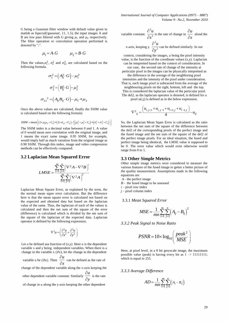
In this section we share one of the image sets we considered

for our experiments (Fig. 1 through Fig. 7). Typically an

image set would comprise of a pair of input images and the set

of 11 fused images produced by each of the fusion algorithms.

Here, we have a pair of input medical images, with one of

them being a CT scan image and the other being MR scan

image.

Fig 1: Pair of medical image input

Fig 2: Fused Image by Average Method (left) and

Maximum Method (right)

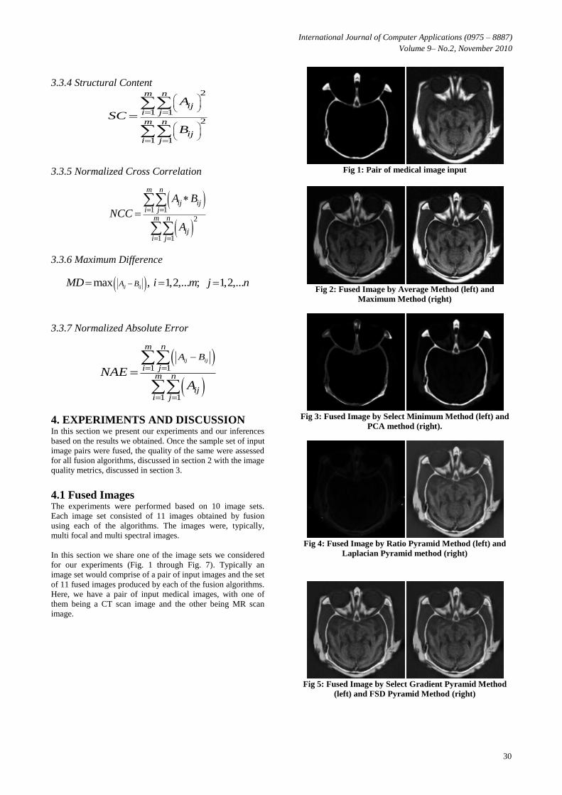
Fig 3: Fused Image by Select Minimum Method (left) and

PCA method (right).

Fig 4: Fused Image by Ratio Pyramid Method (left) and

Laplacian Pyramid method (right)

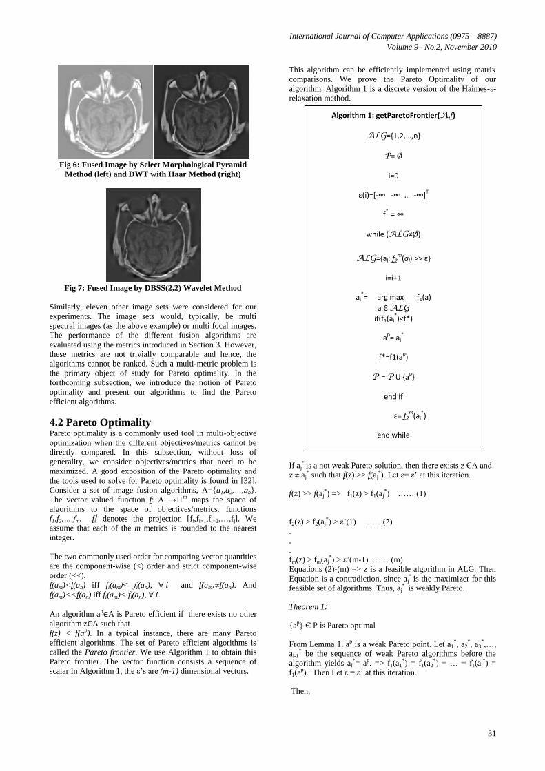
Fig 5: Fused Image by Select Gradient Pyramid Method

(left) and FSD Pyramid Method (right)



31

Fig 6: Fused Image by Select Morphological Pyramid

Method (left) and DWT with Haar Method (right)

Fig 7: Fused Image by DBSS(2,2) Wavelet Method

Similarly, eleven other image sets were considered for our

experiments. The image sets would, typically, be multi

spectral images (as the above example) or multi focal images.

The performance of the different fusion algorithms are

evaluated using the metrics introduced in Section 3. However,

these metrics are not trivially comparable and hence, the

algorithms cannot be ranked. Such a multi-metric problem is

the primary object of study for Pareto optimality. In the

forthcoming subsection, we introduce the notion of Pareto

optimality and present our algorithms to find the Pareto

efficient algorithms.

4.2 Pareto Optimality Pareto optimality is a commonly used tool in multi-objective

optimization when the different objectives/metrics cannot be

directly compared. In this subsection, without loss of

generality, we consider objectives/metrics that need to be

maximized. A good exposition of the Pareto optimality and

the tools used to solve for Pareto optimality is found in [32].

Consider a set of image fusion algorithms, A={a1,a2,…,an}.

The vector valued function f: A →m maps the space of

algorithms to the space of objectives/metrics. functions

f1,f2,…,fm. fij denotes the projection [fi,fi+1,fi+2,…,fj]. We

assume that each of the m metrics is rounded to the nearest

integer.

The two commonly used order for comparing vector quantities

are the component-wise (<) order and strict component-wise

order (<<).

f(am)<f(an) iff fi(am)≤ fi(an), ∀ 𝑖 and f(am)≠f(an). And

f(am)<<f(an) iff fi(am)< fi(an), ∀ 𝑖.

An algorithm ap∈A is Pareto efficient if there exists no other

algorithm z∈A such that

f(z) < f(ap). In a typical instance, there are many Pareto

efficient algorithms. The set of Pareto efficient algorithms is

called the Pareto frontier. We use Algorithm 1 to obtain this

Pareto frontier. The vector function consists a sequence of

scalar In Algorithm 1, the ε’s are (m-1) dimensional vectors.

This algorithm can be efficiently implemented using matrix

comparisons. We prove the Pareto Optimality of our

algorithm. Algorithm 1 is a discrete version of the Haimes-ε-

relaxation method.

If aj* is a not weak Pareto solution, then there exists z ЄA and

z ≠ aj* such that f(z) >> f(aj

*). Let ε= ε’ at this iteration.

f(z) >> f(aj*) => f1(z) > f1(aj

*) …… (1)

f2(z) > f2(aj*) > ε’(1) …… (2)

.

.

.

fm(z) > fm(aj*) > ε’(m-1) …… (m)

Equations (2)-(m) => z is a feasible algorithm in ALG. Then

Equation is a contradiction, since aj* is the maximizer for this

feasible set of algorithms. Thus, aj* is weakly Pareto.

Theorem 1:

{ap} Є P is Pareto optimal

From Lemma 1, ap is a weak Pareto point. Let a1*, a2

*, a3*,…,

al-1* be the sequence of weak Pareto algorithms before the

algorithm yields al*= ap. => f1(a1

*) = f1(a2*) = … = f1(al

*) =

f1(ap). Then Let ε = ε’ at this iteration.

Then,

Algorithm 1: getParetoFrontier(A,f)

ALG=,1,2,…,n-

P= Ø

i=0

ε(i)=*-∞ -∞ … -∞+T

f*

= ∞

while (ALG≠Ø)

ALG={al: f2m

(al) >> ε-

i=i+1

ai*= arg max f1(a)

a Є ALG

if(f1(ai*)<f*)

ap= ai

*

f*=f1(ap)

P = P U {ap}

end if

ε= f2m

(ai*)

end while



32

ap = al* = arg max f1(a) (m+1)

a Є A

f2m(a) >> ε’

Suppose if ap is not Pareto efficient, then there exists z Є A

and z ≠ aj* such that f(z) > f(ap). Since ap is the maximizer for

Equation (m+1), we have

f1(z)=f1(ap),

f2(z) ≥ f2(ap) > ε’(1),

.

.

.

fm(z) ≥ fm(ap) > ε’(m-1), where one of the inequality is true.

Let us assume, with out of loss of generality, f2(z) > f2(ap). Let

ε’’= f2m(ap)=[f2(a

p) ε’’(2) ε’’(3) … ε’’(m-1)], be the threshold

for the next iteration.

For the next iteration, we obtain

a1* = arg max f1(a) (m+1)

a Є A

f2m(a) >> ε’’

Now, a1* must be z, because it satisfies the constraints. But

this is a contradiction. Hence ap is indeed Pareto efficient.

….QED

Thus, Algorithm 1 returns the Pareto frontier. All other

algorithms that are not a part of the Pareto frontier are

dominated by a better algorithm in the Pareto frontier. In other

words, our Pareto method sieves out those algorithms that are

inefficient in the Pareto sense.

The image metrics readings for the twelve image sets were

averaged and the Pareto Frontier was calculated on this

averaged matrix. The method projected DWT with Haar based

fusion method to be efficient, compared to the others, based

on the reading produced by the image quality metrics. The

method also revealed Morphological Pyramid method to be a

dominated algorithm (inferior algorithm).

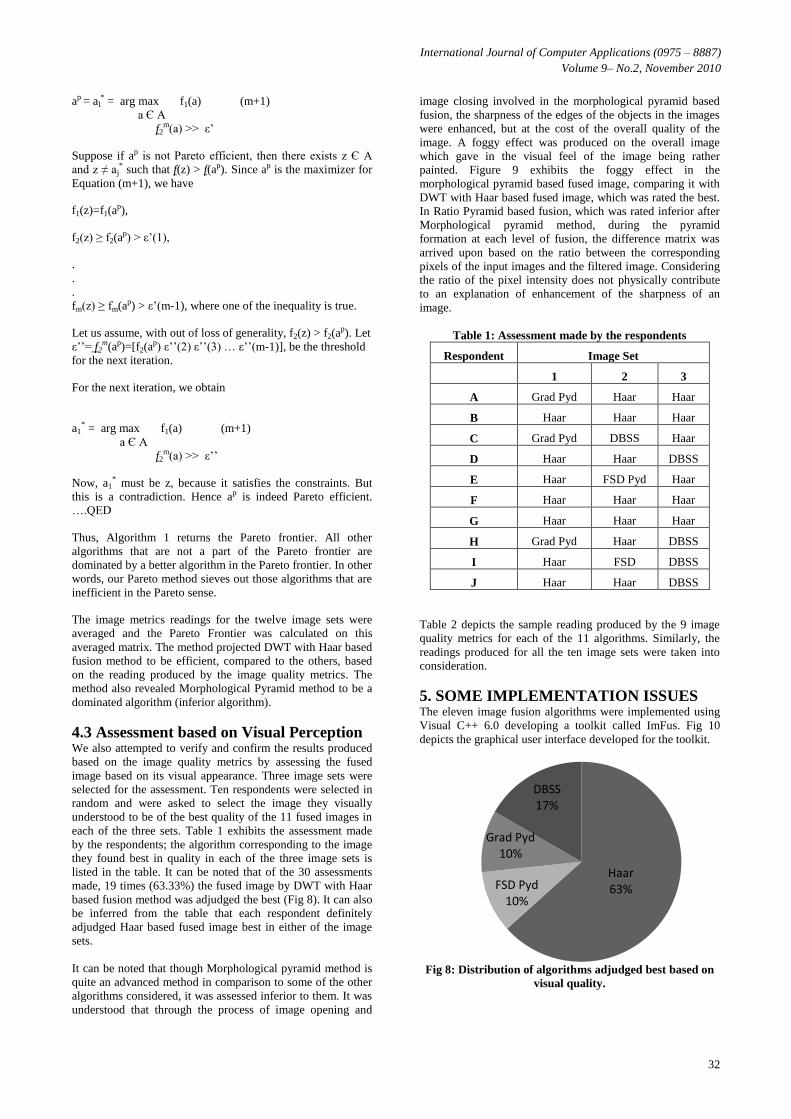
4.3 Assessment based on Visual Perception We also attempted to verify and confirm the results produced

based on the image quality metrics by assessing the fused

image based on its visual appearance. Three image sets were

selected for the assessment. Ten respondents were selected in

random and were asked to select the image they visually

understood to be of the best quality of the 11 fused images in

each of the three sets. Table 1 exhibits the assessment made

by the respondents; the algorithm corresponding to the image

they found best in quality in each of the three image sets is

listed in the table. It can be noted that of the 30 assessments

made, 19 times (63.33%) the fused image by DWT with Haar

based fusion method was adjudged the best (Fig 8). It can also

be inferred from the table that each respondent definitely

adjudged Haar based fused image best in either of the image

sets.

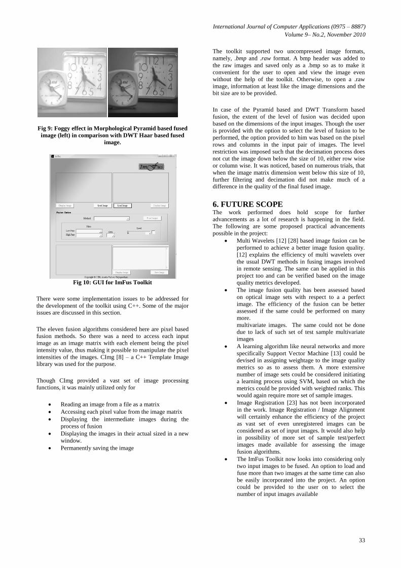
It can be noted that though Morphological pyramid method is

quite an advanced method in comparison to some of the other

algorithms considered, it was assessed inferior to them. It was

understood that through the process of image opening and

image closing involved in the morphological pyramid based

fusion, the sharpness of the edges of the objects in the images

were enhanced, but at the cost of the overall quality of the

image. A foggy effect was produced on the overall image

which gave in the visual feel of the image being rather

painted. Figure 9 exhibits the foggy effect in the

morphological pyramid based fused image, comparing it with

DWT with Haar based fused image, which was rated the best.

In Ratio Pyramid based fusion, which was rated inferior after

Morphological pyramid method, during the pyramid

formation at each level of fusion, the difference matrix was

arrived upon based on the ratio between the corresponding

pixels of the input images and the filtered image. Considering

the ratio of the pixel intensity does not physically contribute

to an explanation of enhancement of the sharpness of an

image.

Table 1: Assessment made by the respondents

Respondent Image Set

1 2 3

A Grad Pyd Haar Haar

B Haar Haar Haar

C Grad Pyd DBSS Haar

D Haar Haar DBSS

E Haar FSD Pyd Haar

F Haar Haar Haar

G Haar Haar Haar

H Grad Pyd Haar DBSS

I Haar FSD DBSS

J Haar Haar DBSS

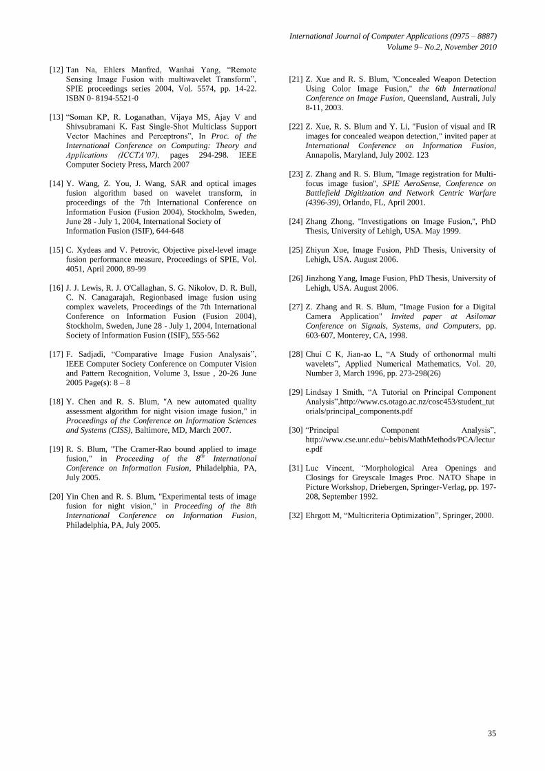
Table 2 depicts the sample reading produced by the 9 image

quality metrics for each of the 11 algorithms. Similarly, the

readings produced for all the ten image sets were taken into

consideration.

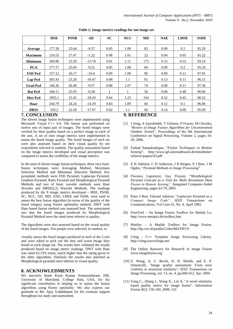
5. SOME IMPLEMENTATION ISSUES The eleven image fusion algorithms were implemented using

Visual C++ 6.0 developing a toolkit called ImFus. Fig 10

depicts the graphical user interface developed for the toolkit.

Fig 8: Distribution of algorithms adjudged best based on

visual quality.

Haar63%FSD Pyd

10%

Grad Pyd10%

DBSS17%



33

Fig 9: Foggy effect in Morphological Pyramid based fused

image (left) in comparison with DWT Haar based fused

image.

Fig 10: GUI for ImFus Toolkit

There were some implementation issues to be addressed for

the development of the toolkit using C++. Some of the major issues are discussed in this section.

The eleven fusion algorithms considered here are pixel based

fusion methods. So there was a need to access each input

image as an image matrix with each element being the pixel

intensity value, thus making it possible to manipulate the pixel

intensities of the images. CImg [8] – a C++ Template Image library was used for the purpose.

Though CImg provided a vast set of image processing

functions, it was mainly utilized only for

Reading an image from a file as a matrix

Accessing each pixel value from the image matrix

Displaying the intermediate images during the

process of fusion

Displaying the images in their actual sized in a new

window.

Permanently saving the image

The toolkit supported two uncompressed image formats,

namely, .bmp and .raw format. A bmp header was added to

the raw images and saved only as a .bmp so as to make it

convenient for the user to open and view the image even

without the help of the toolkit. Otherwise, to open a .raw

image, information at least like the image dimensions and the bit size are to be provided.

In case of the Pyramid based and DWT Transform based

fusion, the extent of the level of fusion was decided upon

based on the dimensions of the input images. Though the user

is provided with the option to select the level of fusion to be

performed, the option provided to him was based on the pixel

rows and columns in the input pair of images. The level

restriction was imposed such that the decimation process does

not cut the image down below the size of 10, either row wise

or column wise. It was noticed, based on numerous trials, that

when the image matrix dimension went below this size of 10,

further filtering and decimation did not make much of a difference in the quality of the final fused image.

6. FUTURE SCOPE The work performed does hold scope for further

advancements as a lot of research is happening in the field.

The following are some proposed practical advancements

possible in the project:

Multi Wavelets [12] [28] based image fusion can be

performed to achieve a better image fusion quality.

[12] explains the efficiency of multi wavelets over

the usual DWT methods in fusing images involved

in remote sensing. The same can be applied in this

project too and can be verified based on the image

quality metrics developed.

The image fusion quality has been assessed based

on optical image sets with respect to a a perfect

image. The efficiency of the fusion can be better

assessed if the same could be performed on many

more.

multivariate images. The same could not be done

due to lack of such set of test sample multivariate

images

A learning algorithm like neural networks and more

specifically Support Vector Machine [13] could be

devised in assigning weightage to the image quality

metrics so as to assess them. A more extensive

number of image sets could be considered initiating

a learning process using SVM, based on which the

metrics could be provided with weighted ranks. This

would again require more set of sample images.

Image Registration [23] has not been incorporated

in the work. Image Registration / Image Alignment

will certainly enhance the efficiency of the project

as vast set of even unregistered images can be

considered as set of input images. It would also help

in possibility of more set of sample test/perfect

images made available for assessing the image

fusion algorithms.

The ImFus Toolkit now looks into considering only

two input images to be fused. An option to load and

fuse more than two images at the same time can also

be easily incorporated into the project. An option

could be provided to the user on to select the

number of input images available



34

Table 2: Image metrics readings for one image set.

MSE PSNR AD SC NCC MD NAE LMSE SSIM

Average 177.28 25.64 -9.57 0.85 1.08 82 0.09 0.2 95.29

Maximum 116.55 27.47 -1.22 0.98 1.01 22 0.04 0.65 91.22

Minimum 304.96 23.29 -13.78 0.81 1.11 175 0.13 0.53 93.16

PCA 177.17 25.64 -9.51 0.85 1.08 84 0.09 0.2 95.24

FSD Pyd 157.12 26.17 -10.4 0.09 1.08 96 0.09 0.13 97.05

Lap Pyd 305.43 23.28 -16.47 0.08 1.1 92 0.13 0.11 96.15

Grad Pyd 146.26 26.48 -9.57 0.86 1.07 74 0.08 0.11 97.36

Rat Pyd 166.11 25.93 -0.58 1 1 56 0.06 0.48 90.06

Mor Pyd 1855.1 15.45 -39.29 0.64 1.23 104 0.32 0.45 86.52

Haar 244.79 24.24 -14.39 0.83 1.09 84 0.12 0.1 96.06

DBSS 359.2 22.58 -17.07 0.82 1.1 66 0.14 0.09 95.09

7. CONCLUSION The eleven image fusion techniques were implemented using

Microsoft Visual C++ 6.0. The fusion was performed on

twelve sets of input pair of images. The fused images were

verified for their quality based on a perfect image in each of

the sets. A set of nine image metrics were implemented to

assess the fused image quality. The fused images of each set

were also assessed based on their visual quality by ten

respondents selected in random. The quality assessment based

on the image metrics developed and visual perception was

compared to assess the credibility of the image metrics.

In the total of eleven image fusion techniques, three very basic

fusion techniques were Averaging Method, Maximum

Selection Method and Minimum Selection Method, five

pyramidal methods were FSD Pyramid, Laplacian Pyramid,

Gradient Pyramid, Ratio Pyramid and Morphological Pyramid

Methods and two of basic wavelet methods were Haar

Wavelet and DBSS(2,2) Wavelet Methods. The readings

produced by the 9 image metrics developed - MSE, PSNR,

SC, NCC, AD, MD, NAE, LMSE and SSIM, were used to

assess the best fusion algorithm (in terms of the quality of the

fused images) using Pareto optimality method. DWT with

Haar based fusion method was assessed best. The assessment

saw that the fused images produced by Morphological

Pyramid Method were the rated most inferior in quality.

The algorithms were also assessed based on the visual quality

of the fused images. Ten people were selected, in random, to

visually assess the fused images produced in each of the 3 sets

and were asked to pick out the best and worst image they

found in each image set. The results here validated the results

produced based on image metric readings. DWT with Haar

was rated 63.33% times, much higher that the rating given to

the other algorithms. Similarly the results also matched as

Morphological pyramid rated inferior in visual quality.

8. ACKNOWLEDMENTS We sincerely thank Kiran Kumar Somasundaram, ISR,

University of Maryland, College Park, USA, for his

significant contribution in helping us to assess the fusion

algorithms using Pareto optimality. We also express our

gratitude to Mr. Ajay Vadakkepatt for his constant support

throughout our study and assessment.

9. REFERENCE

[1] J Zeng, A Sayedelahk, T Gilmore, P Frazier, M Chouika,

“Review of Image Fusion Algorithms for Unconstrained

Outdoor Scenes”, Proceedings of the 8th International

Conference on Signal Processing, Volume 2, pages 16-

20, 2006.

[2] Farhad Samadzadegan, “Fusion Techniques in Remote

Sensing”. http://www.igf.uniosnabrueck.de/mitarbeiter/

schiewe/papers/43.pdf

[3] E H Adelson, C H Anderson, J R Bergen, P J Burt, J M

Ogden, “Pyramid Methods in Image Processing”

[4] Florence Laporterie, Guy Flouzat, “Morphological

Pyramid Concept as a Tool for Multi Resolution Data

Fusion in Remote Sensing”, Integrated Computer-Aided

Engineering, pages 63-79, 2003

[5] Peter J Burt, Edward Adelson, “Laplacian Pyramid as a

Compact Image Code”, IEEE Transactions on

Communications, Vol Com-31, No. 4, April 1983.

[6] FuseTool – An Image Fusion Toolbox for Matlab 5.x,

http://www.metapix.de/toolbox.htm

[7] Matifus – A Matlab Toolbox for Image Fusion,

http://ftp.cwi.nl/pauldz/Codes/MATIFUS

[8] CImg - C++ Template Image Processing Library.

http://cimg.sourceforge.net/

[9] The Online Resource for Research in Image Fusion

www.imagefusion.org

[10] Z. Wang, A. C. Bovik, H. R. Sheikh, and E. P.

Simoncelli, "Image quality assessment: From error

visibility to structural similarity“, IEEE Transactions on

Image Processing, vol. 13, no. 4, pp.600-612, Apr. 2004

[11] Yang C., Zhang J., Wang X., Liu X, "A novel similarity

based quality metric for image fusion". Information

Fusion 9(2): 156-160, 2008. 122

http://ftp.cwi.nl/pauldz/Codes/MATIFUS

http://cimg.sourceforge.net/

http://www.imagefusion.org/



35

[12] Tan Na, Ehlers Manfred, Wanhai Yang, “Remote

Sensing Image Fusion with multiwavelet Transform”,

SPIE proceedings series 2004, Vol. 5574, pp. 14-22.

ISBN 0- 8194-5521-0

[13] “Soman KP, R. Loganathan, Vijaya MS, Ajay V and

Shivsubramani K. Fast Single-Shot Multiclass Support

Vector Machines and Perceptrons”, In Proc. of the

International Conference on Computing: Theory and

Applications (ICCTA’07), pages 294-298. IEEE

Computer Society Press, March 2007

[14] Y. Wang, Z. You, J. Wang, SAR and optical images

fusion algorithm based on wavelet transform, in

proceedings of the 7th International Conference on

Information Fusion (Fusion 2004), Stockholm, Sweden,

June 28 - July 1, 2004, International Society of

Information Fusion (ISIF), 644-648

[15] C. Xydeas and V. Petrovic, Objective pixel-level image

fusion performance measure, Proceedings of SPIE, Vol.

4051, April 2000, 89-99

[16] J. J. Lewis, R. J. O'Callaghan, S. G. Nikolov, D. R. Bull,

C. N. Canagarajah, Regionbased image fusion using

complex wavelets, Proceedings of the 7th International

Conference on Information Fusion (Fusion 2004),

Stockholm, Sweden, June 28 - July 1, 2004, International

Society of Information Fusion (ISIF), 555-562

[17] F. Sadjadi, “Comparative Image Fusion Analysais”,

IEEE Computer Society Conference on Computer Vision

and Pattern Recognition, Volume 3, Issue , 20-26 June

2005 Page(s): 8 – 8

[18] Y. Chen and R. S. Blum, "A new automated quality

assessment algorithm for night vision image fusion," in

Proceedings of the Conference on Information Sciences

and Systems (CISS), Baltimore, MD, March 2007.

[19] R. S. Blum, "The Cramer-Rao bound applied to image

fusion," in Proceeding of the 8th International

Conference on Information Fusion, Philadelphia, PA,

July 2005.

[20] Yin Chen and R. S. Blum, "Experimental tests of image

fusion for night vision," in Proceeding of the 8th

International Conference on Information Fusion,

Philadelphia, PA, July 2005.

[21] Z. Xue and R. S. Blum, ''Concealed Weapon Detection

Using Color Image Fusion,'' the 6th International

Conference on Image Fusion, Queensland, Australi, July

8-11, 2003.

[22] Z. Xue, R. S. Blum and Y. Li, "Fusion of visual and IR

images for concealed weapon detection," invited paper at

International Conference on Information Fusion,

Annapolis, Maryland, July 2002. 123

[23] Z. Zhang and R. S. Blum, ''Image registration for Multi-

focus image fusion'', SPIE AeroSense, Conference on

Battlefield Digitization and Network Centric Warfare

(4396-39), Orlando, FL, April 2001.

[24] Zhang Zhong, ''Investigations on Image Fusion,'', PhD

Thesis, University of Lehigh, USA. May 1999.

[25] Zhiyun Xue, Image Fusion, PhD Thesis, University of

Lehigh, USA. August 2006.

[26] Jinzhong Yang, Image Fusion, PhD Thesis, University of

Lehigh, USA. August 2006.

[27] Z. Zhang and R. S. Blum, "Image Fusion for a Digital

Camera Application" Invited paper at Asilomar

Conference on Signals, Systems, and Computers, pp.

603-607, Monterey, CA, 1998.

[28] Chui C K, Jian-ao L, “A Study of orthonormal multi

wavelets”, Applied Numerical Mathematics, Vol. 20,

Number 3, March 1996, pp. 273-298(26)

[29] Lindsay I Smith, “A Tutorial on Principal Component

Analysis”,http://www.cs.otago.ac.nz/cosc453/student_tut

orials/principal_components.pdf

[30] “Principal Component Analysis”,

http://www.cse.unr.edu/~bebis/MathMethods/PCA/lectur

e.pdf

[31] Luc Vincent, “Morphological Area Openings and

Closings for Greyscale Images Proc. NATO Shape in

Picture Workshop, Driebergen, Springer-Verlag, pp. 197-

208, September 1992.

[32] Ehrgott M, “Multicriteria Optimization”, Springer, 2000.

http://www.cs.otago.ac.nz/cosc453/student_tutorials/principal_components.pdf



http://www.cse.unr.edu/~bebis/MathMethods/PCA/lecture.pdf

http://www.cse.unr.edu/~bebis/MathMethods/PCA/lecture.pdf

implementation and comparative study of image fusion algorithms

Documents