imperial college london - connecting repositories · currently the gas condensate relative...
TRANSCRIPT

IMPERIAL COLLEGE LONDON
Department of Earth Science and Engineering
Centre for Petroleum Studies
How to Model Condensate Banking in a Simulation Model to Get Reliable Forecasts? Case Story of Elgin/Franklin
By
Lionel X. Martinez
A report submitted in partial fulfillment of the requirements for
the MSc and/or the DIC.
September 2011


How to Model Condensate Banking in a Simulation Model? Case Story of Elgin/Franklin i
Declaration Of Own Work
I declare that this thesis:
How to Model Condensate Banking in a Simulation Model to Get Reliable Forecasts? Case Story of Elgin/Franklin
Is entirely my own work and that where any material could be construed as the work of others, it is fully cited and referenced,
and/or with appropriate acknowledgement given.
Signature: .....................................................
Name of student: Lionel X. Martinez
Name of supervisor: Prof. Alain C. Gringarten

How to Model Condensate Banking in a Simulation Model? Case Story of Elgin/Franklin ii
Acknowledgements
This study has been proposed by Elsa Bacchus and Thomas Schaaf at GDF SUEZ E&P UK. I would like to express
my gratitude to them for giving me the opportunity to join their team for the duration of the project and for their patience and
availability that enabled me to achieve the results exposed in this work. I would also like to thank Prof. Gringarten and
Olakunle Ogunrewo for their advices and inputs throughout the project.
This year at Imperial would not have been appreciated as much without the friendship of my fellow Petroleum
Engineering students, as a group we grew stronger and gave ourselves the means to succeed.
Finally, my special thanks go to my former colleagues Paul Cartier and Iskandar Putranto who supported my
application to Imperial College and made my presence as a MSc. Petroleum Engineering candidate possible.

How to Model Condensate Banking in a Simulation Model? Case Story of Elgin/Franklin iii

How to Model Condensate Banking in a Simulation Model? Case Story of Elgin/Franklin iv
Table of Content
Declaration Of Own Work .............................................................................................................................................. i
Acknowledgements ....................................................................................................................................................... ii
List of Figures ............................................................................................................................................................... v
List of Tables ............................................................................................................................................................... vi
Abstract ......................................................................................................................................................................... 1
Introduction ................................................................................................................................................................... 1
Review of existing relative permeability models ........................................................................................................... 2
Current modelling capabilities of the reservoir simulator Eclipse. ................................................................................ 4
Case Study: History matching of the Elgin Field .......................................................................................................... 9
Conclusions ................................................................................................................................................................ 14
Further Work ............................................................................................................................................................... 14
Nomenclature ............................................................................................................................................................. 14
References ................................................................................................................................................................. 15
Appendix ..................................................................................................................................................................... 17
A. Critical Literature Review ....................................................................................................................................... 18
B. Single and Full Field Model Properties, Parameters and Other Results ............................................................... 30
C. Elgin Field Presentation ......................................................................................................................................... 41
D. History matching .................................................................................................................................................... 48
E. LET Correlation ...................................................................................................................................................... 68
F. Other Methods for Well Deliverability Assessment ................................................................................................ 71
G. Other References ................................................................................................................................................... 74
How to Model Condensate Banking in a Simulation Model? Case Story of Elgin/Franklin v
List of Figures Figure 1: Three regions of flow behaviour in a gas-condensate well (Fevang and Whitson, 1996) ............................................... 5 Figure 2: Krg, So profile for Layer 9 after 365 days of production ................................................................................................ 7 Figure 3: Gas Rate/(FPR - BHP) vs. FPR ....................................................................................................................................... 7 Figure 4: GOR evolution ................................................................................................................................................................ 7 Figure 5: Effect of Base Capillary Number on krg (Henderson model) ......................................................................................... 7 Figure 6: Gas Rate/(FPR - BHP) vs. FPR ....................................................................................................................................... 7 Figure 7: Producing GOR ............................................................................................................................................................... 7 Figure 8: Measured GOR evolution for the wells G4, G5 & G7 .................................................................................................... 8 Figure 9: Flux regions of the Elgin Field ........................................................................................................................................ 8 Figure 10: Influence of grid size on GPP well deliverability calculation ....................................................................................... 8 Figure 11: HM-model validation and forecasts generation ............................................................................................................. 9 Figure 12: Assisted History Matching Workflow with CONDOR ............................................................................................... 10 Figure 13: Relative permeability range explored in the optimization (Gas-oil and Water oil relative permeability Tables) ....... 12 Figure 14: Objective function contribution of the different production data in HM 5 .................................................................. 13 Figure B-1: Radial grid (Nr=20; Nz=23) ...................................................................................................................................... 30 Figure B-2: Cartesian grid (Nx=Ny=21, Nz =23) ......................................................................................................................... 30 Figure B-3: Krg evolution with distance (Layer 9 after 365 days of production) – Fine Radial Grid .......................................... 31 Figure B-4: So profile with distance (Layer 9 after 365 days of production) – Fine Radial Grid ................................................ 32 Figure B-5: Kro profile (Layer 9 after 365 days of production) – Fine Radial Grid .................................................................... 32 Figure B-6: Near-Well (Nr=1) So, Krg, Pressure profile along depth after 365 days of production – Fine Radial Grid ............. 33 Figure B-7: Base Capillary Number effect on productivity .......................................................................................................... 39 Figure B-8: Effect of modelling only krg or krg and kro .............................................................................................................. 39 Figure B-9: Sensitivity of well productivity as a function of n1 ................................................................................................... 39 Figure B-10: Gas Production Rate simulated with the different models in FFM ......................................................................... 40 Figure C-1: Overview of the Elgin Field panels in the reservoir model ....................................................................................... 41 Figure C-2: Elgin-West PVT Phase envelope.............................................................................................................................. 42 Figure C-3: Elgin-West Liquid condensation curve ..................................................................................................................... 42 Figure C-4: Elgin Field Gas Production Rates.............................................................................................................................. 43 Figure C-5: Elgin Field Water Production Rates .......................................................................................................................... 43 Figure C-6: Elgin Field Historical Production Rate ...................................................................................................................... 44 Figure C-7: Well G4 Tubing Head Pressure (THP, BARA) historical data ................................................................................. 44 Figure C-8: Well G4 GOR historical data .................................................................................................................................... 44 Figure C-9: Elgin Faults ............................................................................................................................................................... 47 Figure C-10: Well G6 Watering from the West in the simulation model (Open Fault) ................................................................ 47 Figure C-11: Impact of fault closure on simulated G6 water production ..................................................................................... 47 Figure D-1: Computation of gradients with two parameters x1 and x2 (Source: Condor v 2.6 documentation) ........................... 48 Figure D-2: Plurigaussian technique applied to the facies realization in the Elgin Field HM 2 ................................................... 49 Figure D-3: Gradual deformations on a FFTMA exponential facies realization .......................................................................... 49 Figure D-4: Definition of a Facies Proportions Transformation ................................................................................................... 50 Figure D-5: Illustration of the Facies Proportion Transformation ................................................................................................ 50 Figure D-6: Optimization workflow used in Condor for the Assisted History Matching HM1 ................................................... 51 Figure D-7: Reservoir structure description in Condor R&D ....................................................................................................... 52 Figure D-8: Determination of base value for log(K) = f(phi) function ......................................................................................... 53 Figure D-9: Upscaled Porosity realization for simplified two facies model ................................................................................. 53 Figure D-10: Objective Function Evolution for HM 1 (109 iterations) ........................................................................................ 54 Figure D-11: Objective Function Evolution for HM 2 (66 iterations) .......................................................................................... 56 Figure D-12: Relative contribution of the different data to the Objective Function value (HM2). .............................................. 56 Figure D-13: Contribution of the different data to the Objective Function value (HM2). ............................................................ 57 Figure D-14: Upscaled porosity realization for HM 3 .................................................................................................................. 59 Figure D-15: Objective function evolution for the optimization HM3 (123 iterations) ................................................................ 59
How to Model Condensate Banking in a Simulation Model? Case Story of Elgin/Franklin vi
Figure D-16: Relative contribution of the different production data available for the objective function calculation (HM3) ..... 60 Figure D-17: Contribution of the different production data available for the objective function calculation (HM3) ................... 60 Figure D-18: Contribution of the G8 BHP measurement to the objective function (HM3). ......................................................... 61 Figure D-19: G8 BHP simulated vs. observed for iteration #65 (HM3). ...................................................................................... 62 Figure D-20: Region for Local Grid Deformations ...................................................................................................................... 63 Figure D-21: Objective function evolution for the optimization HM4 (100 iterations) ................................................................ 64 Figure D-22: Relative contribution of the different production data available for the objective function calculation (HM4) ..... 64 Figure D-23: Contribution of the different production data available for the objective function calculation (HM4) ................... 64 Figure D-24: Objective function evolution for the optimization HM5 (122 iterations) ................................................................ 66 Figure D-25: Relative contribution of the different production data available for the objective function calculation (HM5) ..... 66 Figure D-26: Relative contribution of the different production data available for the objective function calculation (HM5) ..... 66 Figure F-1: Well productivity for different non-Darcy flow models ............................................................................................ 73 List of Tables Table 1: Review of parameters and objective function definition for each HM attempt .............................................................. 11 Table 2: Relative permeability optimization parameters .............................................................................................................. 12 Table B-1: PVT Properties ........................................................................................................................................................... 30 Table B-2: Layer Properties .......................................................................................................................................................... 30 Table B-3: Radial grid dimensions (Dr) ....................................................................................................................................... 30 Table B-4: Cartesian grid dimensions........................................................................................................................................... 30 Table B-5: Rich gas condensate parameters used for Base Case9 (Henderson model) ................................................................. 31 Table C-1: Elgin Field wells first production dates ...................................................................................................................... 41 Table C-2: Elgin West Gas composition ...................................................................................................................................... 42 Table C-3: Elgin Field regions temperature .................................................................................................................................. 45 Table C-4: Reservoir Properties (Source: Operator Reports) ....................................................................................................... 46 Table C-5: Porosity trend along Z (% per 100 meters) ................................................................................................................. 46 Table C-6: Facies Proportions ...................................................................................................................................................... 46 Table C-7: Faults impact on dynamic simulation behaviour ........................................................................................................ 47 Table D-1: ECLIPSE and CONDOR geomodel grid dimensions................................................................................................. 51 Table D-2: Match quality evolution for FGPT and FWPT between first and optimum iterations (HM1). ................................... 55 Table D-3: Match quality evolution for FGPT and FWPT between first and optimum iterations (HM2). ................................... 58 Table D-4: Match quality evolution for FGPT and FWPT between first and optimum iterations (HM3). ................................... 61 Table D-5: Match quality evolution for the well G8 BHP and WGPT between first and optimum iterations (HM3). ................ 62 Table D-6: Match quality evolution for FGPT and FWPT between first and optimum iterations (HM4). ................................... 65 Table D-7: Match quality evolution for FGPT and FWPT between first and optimum iterations (HM5). ................................... 67

How To Model Condensate Banking In A Simulation Model To Get Reliable Forecasts? Case Story Of Elgin/Franklin Lionel Xavier Martinez
Imperial College supervisor: Prof. Alain C. Gringarten
Company supervisor: Elsa Bacchus and Thomas Schaaf, GDF SUEZ E&P UK
Abstract Condensate banking has started in 2008 in the Elgin field and is expected to cause more than 20% liquid dropout in the pore volume. The need to generate reliable forecasts prompted the study of condensate banking modelling for the Elgin Field. A review of the existing models for gas-condensate relative permeability and modelling was performed, exploring the current capabilities of the commercial reservoir simulator ECLIPSE. The quality of the forecasts is also linked to the history matched models chosen. In order to study how to obtain several history matched models the assisted history matching tool CONDOR (CONstrained Description Of Reservoir) was used.
Currently the gas condensate relative permeability models of Whitson and Fevang (1999) and Henderson (2000) are available in the reservoir simulator Eclipse. Both these models rely on interpolation of the relative permeability between miscible and immiscible relative permeability curves and are dependent on the capillary number. The study of the condensate banking effects on single well models showed that the impairment of well productivity due to condensate banking in the Elgin Field should be limited. However the physical aspect of condensate banking needs to be properly captured in the model to avoid overestimating the impact. At the full field scale, the current reservoir model showed little sensitivity to the inclusion of the capillary number modified relative permeability when using the pseudopressure computation for well productivity. However due to the lack of experimental data for the Elgin field further investigations need to be performed to properly determine the model parameters, notably through performing core experiments or well tests.
History matching is a necessary exercise to perform before being able to produce reliable production forecasts. The improvements in assisted history matching tools enabled extending the goals of the exercise to obtaining several history matched models. However the use of CONDOR to perform assisted history matching highlighted the difficulty to reconcile the need for a large number of static and dynamic variables with obtaining satisfactory match for different types of reservoir data. The assisted history matching proved efficient to optimize the geological and dynamic simulation models against a single type of production data (e.g. the cumulative field gas production). The need to select the relevant production data (e.g. problem of uncertainty on the back allocated production rates in the Elgin Field) and their associated weights for the objective function definition was shown to be necessary to get sound matches within a reasonable timeframe. Introduction The Elgin field is a high pressure high temperature (HPHT) rich gas condensate field located in the Central North Sea with an initial reservoir pressure of 1100 bars and a temperature of 190 ºC. The reservoir was discovered in 1991 and has been producing since 2001. The field has presented considerable development challenges due to its HPHT conditions. Eight production wells were drilled and the reservoir fluids have been produced using pressure depletion.
The PVT analysis of the reservoir fluids predicts a dew point pressure of 325 Bars. This implies that the pressure around the wells should have fallen below the dew point in 2008. However no effects on well productivity have been clearly identified. This raised questions about the PVT analysis previously performed and concerns about the potential impact of condensation on future production.
The major production of the field comes from the Fulmar formation (Franklin sands) subdivided into three stratigraphic units: the Franklin A, B and C sands, the B sands being the main contributor. Previous studies conducted by Mott (2006) on behalf of the operator had concluded that the condensate blockage should have only a small impact on well deliverability due to the combination of high permeability and thickness in the reservoir. The observation of current back allocated production confirms that no obvious effect of condensate banking can be seen; however its impact cannot be fully ruled out (more than 20% liquid dropout is expected). As a partner GDF SUEZ E&P UK needs to be able to verify the assumption of condensate banking in the reservoir model. Currently condensate banking is taken into account in the dynamic reservoir model through a reduction of oil mobility around the wells. It does not account for enhancement in relative
How to Model Condensate Banking in a Simulation Model? Case Story of Elgin/Franklin 2
permeability associated with viscous forces and it is anticipated that as the pressure in the reservoir drops, the simulation model predictions may deviate from the observed data.
Reliable forecasts are necessary to predict future income from operations. As history matching is an underdetermined inverse problem, an infinite number of matching models exists. Therefore the availability of multiple history matched models to assess uncertainty in the forecast is necessary. One way of obtaining history matched models is to use assisted history matching tools. The recent advances in assisted history matching have led to the development of software enabling to explore the uncertain parameters possible values in both the geological and dynamic simulation model through the history matching process. CONDOR (CONstrained Description Of Reservoir) is a versatile history matching software giving the engineer control over the convergence criteria (Objective Function) and optimization parameters that can be defined in both the geomodelling and dynamic simulation process (IFP, 2011).
The objectives of this project are: to perform a technical review of the existing condensate relative permeability models and of the current modelling capabilities of the commercial reservoir simulator ECLIPSE (version 2009.2); to investigate alternative geological and simulation models for history matching of the Elgin field using assisted history matching tools (CONDOR Research Prototype v2.6) and obtain a series of suitable history matched models for production forecasts. Review of existing relative permeability models The modelling of condensate banking effects on well production is still an area of development in reservoir engineering. Well productivity is expected to decline as the pressure falls below the dew point due to the accumulation of condensate around the wellbore. However it is difficult to assess the effects of condensate banking without the acquisition of specific core, PVT and well production data in order to accurately model the condensation effects on gas relative permeability and production. Measurements of gas-condensate relative permeability at reservoir conditions for a field like Elgin is very difficult and requires expensive laboratory data; well test data is also difficult to acquire given the high temperature of the reservoir. Dependency of gas-condensate relative permeability on the capillary number. Laboratory experiments have demonstrated that condensate relative permeability can increase significantly with increasing rate; important variables like the velocity, the capillary forces and the interfacial tension between the gas and the condensate have been identified. It is recognized that in the near-wellbore region the balance of viscous forces and capillary forces is reversed as the interfacial tension decreases once the pressure falls below the dew point and the viscous forces increase with velocity. Therefore the effects that should reduce well productivity (capillary forces) are balanced by effects that improve well productivity (viscous forces).
The capillary number is defined as the ratio of viscous to capillary effects. The flow properties become thus dependent on the capillary number. The viscous forces enhance the relative permeability, straightening the curves towards miscible relative permeability at high capillary number, this phenomenon is also known as “positive coupling”. At low capillary number the gas condensate relative permeability tends towards the immiscible curve.
Many correlations and models have been proposed in the literature to link the relative permeability of gas condensate to the capillary number. Blom and Hagoort (1998) proposed their own correlation and analysed fifteen different methods to include the capillary number in the gas condensate relative permeability functions. They divided the methods in two classes: one using Corey functions in which the Corey coefficients are interpolated between immiscible and miscible limits,
𝑘𝑘𝑟𝑟𝑟𝑟�𝑆𝑆𝑟𝑟,𝑁𝑁𝑐𝑐� = 𝑘𝑘𝑟𝑟𝑟𝑟∗ (𝑁𝑁𝑐𝑐)�𝑆𝑆𝑟𝑟 − 𝑆𝑆𝑟𝑟𝑟𝑟(𝑁𝑁𝑐𝑐)1 − 𝑆𝑆𝑟𝑟𝑟𝑟(𝑁𝑁𝑐𝑐) �
𝜀𝜀𝑝𝑝(𝑁𝑁𝑐𝑐)
. . . . . equation 1
and the other using an interpolation function between integral immiscible and miscible relative permeability curves. 𝑘𝑘𝑟𝑟𝑟𝑟�𝑆𝑆𝑟𝑟,𝑁𝑁𝑐𝑐� = 𝑓𝑓𝑟𝑟(𝑁𝑁𝑐𝑐)𝑘𝑘𝑟𝑟𝑟𝑟𝑟𝑟�𝑆𝑆𝑟𝑟�+ �1 − 𝑓𝑓𝑟𝑟(𝑁𝑁𝑐𝑐)�𝑘𝑘𝑟𝑟𝑟𝑟𝑟𝑟�𝑆𝑆𝑟𝑟� . . . . . equation 2
In both classes of studied methods the interpolation is weighted by capillary number dependent functions. Blom and Hagoort (1998) cited some advantages of using the capillary number dependent Corey functions but identified important disadvantages: it is difficult to fit the resulting functions to a large quantity of data and the Corey function cannot represent S-shape relative permeabilities that have been reported in some cases (the kind that is currently in use in the Elgin field model).The interpolation method between immiscible and miscible relative permeability curves uses a weighting function dependent on the capillary number. This method is applicable to a great quantity of measured data and is more efficient than the interpolation with Corey coefficients.
Finally the authors have been able to identify three different weighting functions they estimated most suitable and found the weighting function proposed by Whitson and Fevang (1999), currently implemented in the commercial reservoir simulator ECLIPSE, to be the most convenient as it covers the entire range of capillary numbers and is able to reproduce the most important aspects of the dependence of relative permeability on the capillary number with a limited number of parameters.
Whitson and Fevang correlation (1999). Following special steady-state experiments to measure krg as a function of krg/kro and the capillary number, the authors developed a capillary number modified gas relative permeability correlation as an interpolation between the straight-line miscible relative permeability and the immiscible relative permeability. It depends only on two parameters (𝑛𝑛,𝛼𝛼𝑐𝑐0) that should be experimentally determined (the authors have proposed the values 0.65 and 104 for 𝑛𝑛 and 𝛼𝛼𝑐𝑐0 respectively). The interpolation is controlled by a transition function 𝑓𝑓𝑟𝑟 and is described in equation 3:

How to Model Condensate Banking in a Simulation Model? Case Story of Elgin/Franklin 3
𝑘𝑘𝑟𝑟𝑟𝑟 = 𝑓𝑓𝑟𝑟𝑘𝑘𝑟𝑟𝑟𝑟𝑟𝑟 + (1 − 𝑓𝑓𝑟𝑟)𝑘𝑘𝑟𝑟𝑟𝑟𝑟𝑟 . . . . . equation 3 with:
𝑓𝑓𝑟𝑟 =1
(𝛼𝛼.𝑁𝑁𝑐𝑐)𝑛𝑛 + 1 . . . . . equation 4
𝛼𝛼 =𝛼𝛼0
𝑘𝑘𝑟𝑟𝑟𝑟����� with 𝑘𝑘𝑟𝑟𝑟𝑟����� =𝑘𝑘𝑟𝑟𝑟𝑟𝑟𝑟 + 𝑘𝑘𝑟𝑟𝑟𝑟𝑟𝑟
2 . . . . . equation 5
𝛼𝛼0 =𝛼𝛼𝑐𝑐0
�𝐾𝐾.𝜑𝜑 . . . . . equation 6
Subsequently more relative permeability correlations for gas condensate systems have been proposed (Henderson et al. 2000, Jamiolahmady, et al. 2003, Bang, et al. 2006) and companies have developed their own in-house correlations (Ayyalasomayajula, Silpngarmlers and Kamath 2005).The correlation from Henderson et al. (2000) allows a broad control on the interpolation parameters and is available in the commercial reservoir simulator ECLIPSE. It will therefore be introduced.
Henderson et al. correlation (2000). The authors have reported their observations of increasing condensing fluids
relative permeability with increasing velocity at conditions where inertia is not significant. Their experimens were realized with dry gas on different types of lithology using steady-state flow experiments. They developed a correlation accounting for both positive coupling and negative inertia effects that they tested against their experiments. The capillary number modified relative permeability for the phase p is defined as: 𝑘𝑘𝑟𝑟𝑟𝑟𝑟𝑟 = 𝑌𝑌𝑘𝑘𝑟𝑟𝑟𝑟𝑟𝑟 + (1 − 𝑌𝑌)𝑘𝑘𝑟𝑟𝑟𝑟𝑟𝑟 . . . . . equation 7
with
𝑌𝑌 = �𝑁𝑁𝑐𝑐𝑐𝑐𝑟𝑟𝑁𝑁𝑐𝑐𝑟𝑟
�1/𝑛𝑛𝑝𝑝
. . . . . equation 8
𝒏𝒏𝒑𝒑 = 𝒏𝒏𝟏𝟏𝒑𝒑𝑺𝑺𝒑𝒑𝒏𝒏𝟐𝟐𝒑𝒑 . . . . . equation 9
𝑺𝑺𝒓𝒓𝒑𝒑𝒓𝒓∗ = 𝑺𝑺𝒓𝒓𝒑𝒑𝒓𝒓�𝟏𝟏 − 𝒆𝒆−𝒎𝒎𝒑𝒑𝑵𝑵𝒄𝒄𝒏𝒏𝒑𝒑� . . . . . equation 10
𝒌𝒌𝒓𝒓𝒑𝒑𝒓𝒓 =�𝑺𝑺𝒑𝒑 − 𝑺𝑺𝒓𝒓𝒑𝒑𝒓𝒓∗ ��𝟏𝟏 − 𝑺𝑺𝒓𝒓𝒑𝒑𝒓𝒓∗ �
. . . . . equation 11
𝑵𝑵𝒄𝒄𝒏𝒏𝒑𝒑 = 𝑵𝑵𝒄𝒄𝒄𝒄𝒑𝒑𝑵𝑵𝒄𝒄𝒑𝒑
. . . . . equation 12
where 𝑛𝑛1𝑟𝑟, 𝑛𝑛2𝑟𝑟and 𝑚𝑚𝑟𝑟 are experimentally determined parameters
Other models. It has been shown that capillary forces alone may not be sufficient to provide a satisfactory parameterization of the relative permeability. Pope, et al. (1998) proposed a simple two-parameter capillary trapping model derived from the approach first used by Delshad et al. (1986). The model allows computing the gas and condensate relative permeability as a function of the trapping number. The trapping number is a generalization of the capillary and the bond (ratio of gravity to capillary forces) numbers. The model was checked against experimental data and the authors identified a general trend of increasing endpoint relative permeability with increasing trapping number and the endpoint can be close to one for sufficiently high trapping number. They justify the use of the trapping number because even with high interfacial tension (low capillary number) the trapping number can still be made high enough to make the endpoint approach a value of one, showing that the interfacial tension is not always the most influential parameter. The bond and trapping numbers are defined as follows (Pope, et al. 1998):
𝑁𝑁𝐵𝐵 =𝑘𝑘𝑘𝑘𝑘𝑘𝑘𝑘𝜎𝜎 . . . . . equation 13
𝑵𝑵𝑻𝑻 =�𝒌𝒌��⃗��⃗ . �𝜵𝜵��⃗ 𝜱𝜱 + 𝒈𝒈𝒈𝒈𝒈𝒈𝜵𝜵��⃗ 𝑫𝑫��
𝝈𝝈 . . . . . equation 14
where 𝛻𝛻�⃗ 𝛷𝛷 is the flow potential gradient. Vizika and Kalaydjian (2002) also developed a calculation method combining the effects of capillary, viscous and
gravity forces on gas condensate mobility. Their model is based on the dependence of the relative permeability and condensate mobility on the capillary number and the bond number and includes the structure characteristics of the porous medium through its fractal dimension. They describe three regions around the well in terms of capillary number and bond number values. The near well bore region exhibits high velocity and high interfacial tension (high capillary number, low bond number), the reservoir with low velocity and intermediate interfacial tension (low capillary number, high bond number) and the near-critical reservoir with low velocity and low interfacial tension (high capillary number, high bond number). In their work they were able to identify and predict the threshold condensate saturation, Stc, below which the condensate mobility is very small, even though finite. The critical saturation for condensate mobility, Scc, increases with interfacial tension (decreasing bond number) and

How to Model Condensate Banking in a Simulation Model? Case Story of Elgin/Franklin 4
fractal dimension (i.e. clay content for sandstones). The model proposed by Vizika and Kalaydjian (2002) was able to satidfactorily match experimental results.
Areas of research. Another standpoint currently being researched is the modelling of the effects of composition on
relative permeability for multiphase flow with mass transfer (Yuan and Pope 2011). This model expresses the relative permeability values as a continuous function of the molar Gibbs free energy of each phase so they will be independent of the phase identity.
Current modelling capabilities of the commercial reservoir simulator used. Available models. In the commercial reservoir simulator ECLIPSE (2009) the relative permeability correlations proposed by Henderson et al. and Whitson and Fevang are available and can be accessed through the keyword VELDEP, they fall under the Non-Darcy Flow, velocity dependent relative permeability category. Both these correlations define a correlation function dependent on the capillary number as discussed previously. These models will affects the residual saturations defined by the user and interpolate the relative permeability between the immiscible and miscible relative permeability.
In the present study the definition of the capillary number given in equation 15 is used as it was originally used by Henderson et al. (2000) and Whitson and Fevang (1999) in their correlations and is the most encountered in the literature. Given the absence of relevant well test and core experimental data for this case study, the base capillary number has been estimated in Appendix B-2.
𝑵𝑵𝒄𝒄𝒑𝒑 =𝒗𝒗𝒈𝒈𝝁𝝁𝒈𝒈𝝈𝝈 . . . . . equation 15
The velocity dependent relative permeability are to be used in fine scale grid in order to avoid averaging of the pressure over a large volume which would result in inaccurate saturation, pressure and flow calculations in the near-wellbore region where condensate is present. The VELDEP option can be combined in coarse grid models with the generalized pseudo-pressure calculation option for well deliverability (Fevang and Whitson 1995).
Henderson et al. correlation. The Henderson correlation (2000, cf. equation 7) can be applied in the reservoir simulator ECLIPSE through the items 1 and 2 of the VELDEP keyword (item 1 for the oil phase and 2 for the gas phase). It requires the input of the immiscible relative permeability curves in the model. The parameters 𝑛𝑛1𝑟𝑟, 𝑛𝑛2𝑟𝑟, 𝑚𝑚𝑟𝑟and Ncbp should be provided for each relative permeability table defined and should have been determined experimentally. They can be controlled in the simulator through the items 1,2,3 and 4 respectively of the keywords VDRKG and VDKRO. Due to the lack of experimental data in this case study they will be taken from the literature for a rich gas condensate9 (cf. Table B-5).
Whitson et al. correlation. The correlation has been described in equation 3; it can only be activated for the gas phase through the item 5 of the keyword VELDEP and can be combined with the Henderson model for the capillary number modified oil relative permeability (item 1). The capillary number for the gas phase is computed using equation 15. It requires the input of the immiscible relative permeability curves in the model. It does not affect residual saturation, does not account have a lower threshold for capillary number (base capillary number) and depends only two parameters (𝑛𝑛, 𝛼𝛼𝑐𝑐0) that can be set to the default values (0.65 and 104 respectively) in the simulator which make it more simple to handle. The gas capillary number is calculated from Model 1 (equation 15), using a pore gas velocity:
𝑣𝑣𝑟𝑟𝑟𝑟 =𝑣𝑣𝑟𝑟
𝜑𝜑. (1 − 𝑆𝑆𝑤𝑤) . . . . . equation 16
The values of (𝑛𝑛, 𝛼𝛼𝑐𝑐0) can be modified through the items 1 and 2 of the keyword VDKRGC for each relative permeability table defined.
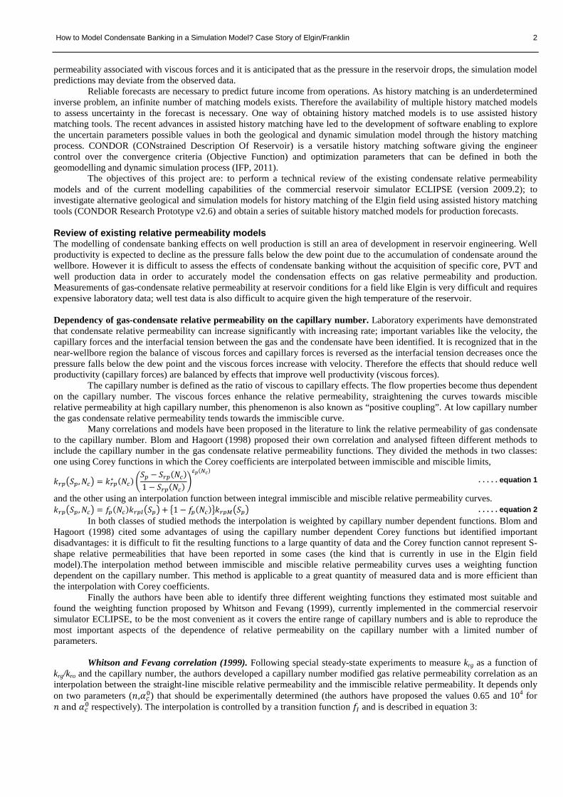
Pseudopressure integral for gas-condensate well deliverability calculation. A method for modelling the deliverability of gas condensate wells in coarse grid model has been implemented in the commercial reservoir simulator ECLIPSE. It can be called for all the wells through the keyword PSEUPRES or invoked for individual wells through entering ‘GPP’ in item 8 of the well definition items in the keyword WELLSPECS. It relies on Fevang and Whitson definition of the three main flow regions for the flow toward a gas-condensate producing well. As mentioned this computation method can be combined with the calculation of velocity dependent relative permeability. It allows obtaining satisfying results for coarse grid models matching those obtained using local grid refinement and conventional flow calculation. This option removes the need of local grid refinement around the wells to model the condensate banking effects on deliverability and thus allows considerable gains in computation time for large field models. Fevang and Whitson described the three flow regions (cf. Figure 1) as follows:
Region 1. In region 1 multiphase flow of oil and gas can be observed with no change in composition in the entire region. Therefore the composition of the gas coming into region 1 is the same as the composition of the produced gas at the well. Knowing the composition of the produced gas thus allows knowing the composition of the gas flowing in the region 1. At the outer edge of this region the pressure is equal to the dew point of the flowing mixture. This region is growing with
How to Model Condensate Banking in a Simulation Model? Case Story of Elgin/Franklin 5
production time and it is where most of the deliverability loss occurs. The liquid saturation distribution in this region affects the gas relative permeability.
Region 2. It can be defined as a condensation zone: the liquid condensate does not flow but keeps accumulating as the gas streams. It defines a region of net accumulation of condensate as the oil has not yet reached the critical saturation to be able to flow; therefore the oil is not or barely movable. The pressure at the outer edge is the dew point pressure of the reservoir gas. The saturations in hydrocarbon fluids can be obtained through the liquid dropout curve obtained from the simulation of a constant-volume depletion (CVD) experiment, corrected for water saturation.
Region 3. It represents the area of the reservoir where pressure has not yet fallen below the dew point. The flow simulation in Region 3 can thus be performed using the theories applicable for single phase gas flow.
Figure 1: Three regions of flow behaviour in a gas-condensate
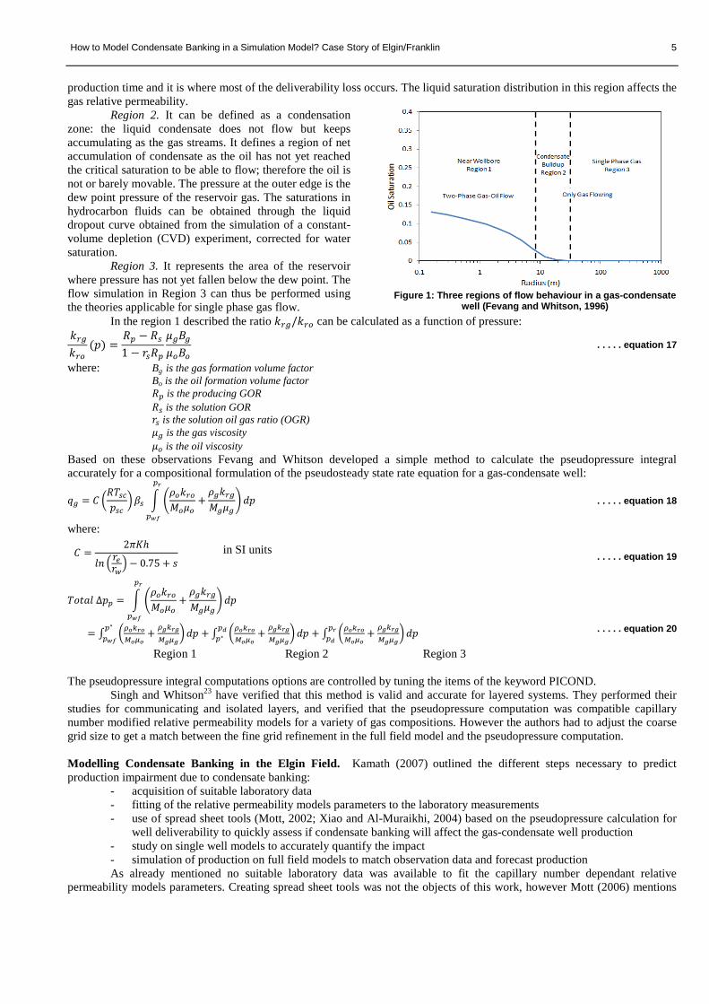
well (Fevang and Whitson, 1996) In the region 1 described the ratio 𝑘𝑘𝑟𝑟𝑟𝑟/𝑘𝑘𝑟𝑟𝑟𝑟 can be calculated as a function of pressure:
𝑘𝑘𝑟𝑟𝑟𝑟𝑘𝑘𝑟𝑟𝑟𝑟
(𝑝𝑝) =𝑅𝑅𝑟𝑟 − 𝑅𝑅𝑠𝑠1 − 𝑟𝑟𝑠𝑠𝑅𝑅𝑟𝑟
𝜇𝜇𝑟𝑟𝐵𝐵𝑟𝑟𝜇𝜇𝑟𝑟𝐵𝐵𝑟𝑟
. . . . . equation 17
where: Bg is the gas formation volume factor Bo is the oil formation volume factor 𝑅𝑅𝑟𝑟 is the producing GOR 𝑅𝑅𝑠𝑠 is the solution GOR 𝑟𝑟𝑠𝑠 is the solution oil gas ratio (OGR) 𝜇𝜇𝑟𝑟 is the gas viscosity 𝜇𝜇𝑟𝑟 is the oil viscosity Based on these observations Fevang and Whitson developed a simple method to calculate the pseudopressure integral accurately for a compositional formulation of the pseudosteady state rate equation for a gas-condensate well:
𝑞𝑞𝑟𝑟 = 𝐶𝐶 �𝑅𝑅𝑇𝑇𝑠𝑠𝑐𝑐𝑝𝑝𝑠𝑠𝑐𝑐
� 𝛽𝛽𝑠𝑠 � �𝑘𝑘𝑟𝑟𝑘𝑘𝑟𝑟𝑟𝑟𝑀𝑀𝑟𝑟𝜇𝜇𝑟𝑟
+𝑘𝑘𝑟𝑟𝑘𝑘𝑟𝑟𝑟𝑟𝑀𝑀𝑟𝑟𝜇𝜇𝑟𝑟
�
𝑟𝑟𝑟𝑟
𝑟𝑟𝑤𝑤𝑤𝑤
𝑑𝑑𝑝𝑝 . . . . . equation 18
where:
𝐶𝐶 =2𝜋𝜋𝐾𝐾ℎ
𝑙𝑙𝑛𝑛 �𝑟𝑟𝑒𝑒𝑟𝑟𝑤𝑤� − 0.75 + 𝑠𝑠
in SI units . . . . . equation 19
𝑇𝑇𝑇𝑇𝑇𝑇𝑇𝑇𝑙𝑙 ∆𝑝𝑝𝑟𝑟 = � �𝑘𝑘𝑟𝑟𝑘𝑘𝑟𝑟𝑟𝑟𝑀𝑀𝑟𝑟𝜇𝜇𝑟𝑟
+𝑘𝑘𝑟𝑟𝑘𝑘𝑟𝑟𝑟𝑟𝑀𝑀𝑟𝑟𝜇𝜇𝑟𝑟
�
𝑟𝑟𝑟𝑟
𝑟𝑟𝑤𝑤𝑤𝑤
𝑑𝑑𝑝𝑝
= ∫ �𝜌𝜌𝑜𝑜𝑘𝑘𝑟𝑟𝑜𝑜𝑟𝑟𝑜𝑜𝜇𝜇𝑜𝑜
+ 𝜌𝜌𝑔𝑔𝑘𝑘𝑟𝑟𝑔𝑔𝑟𝑟𝑔𝑔𝜇𝜇𝑔𝑔
�𝑟𝑟∗
𝑟𝑟𝑤𝑤𝑤𝑤𝑑𝑑𝑝𝑝 + ∫ �𝜌𝜌𝑜𝑜𝑘𝑘𝑟𝑟𝑜𝑜
𝑟𝑟𝑜𝑜𝜇𝜇𝑜𝑜+ 𝜌𝜌𝑔𝑔𝑘𝑘𝑟𝑟𝑔𝑔
𝑟𝑟𝑔𝑔𝜇𝜇𝑔𝑔�𝑟𝑟𝑑𝑑
𝑟𝑟∗ 𝑑𝑑𝑝𝑝 + ∫ �𝜌𝜌𝑜𝑜𝑘𝑘𝑟𝑟𝑜𝑜𝑟𝑟𝑜𝑜𝜇𝜇𝑜𝑜
+ 𝜌𝜌𝑔𝑔𝑘𝑘𝑟𝑟𝑔𝑔𝑟𝑟𝑔𝑔𝜇𝜇𝑔𝑔
�𝑟𝑟𝑟𝑟𝑟𝑟𝑑𝑑
𝑑𝑑𝑝𝑝
. . . . . equation 20
Region 1 Region 2 Region 3 The pseudopressure integral computations options are controlled by tuning the items of the keyword PICOND.
Singh and Whitson23 have verified that this method is valid and accurate for layered systems. They performed their studies for communicating and isolated layers, and verified that the pseudopressure computation was compatible capillary number modified relative permeability models for a variety of gas compositions. However the authors had to adjust the coarse grid size to get a match between the fine grid refinement in the full field model and the pseudopressure computation. Modelling Condensate Banking in the Elgin Field. Kamath (2007) outlined the different steps necessary to predict production impairment due to condensate banking:
- acquisition of suitable laboratory data - fitting of the relative permeability models parameters to the laboratory measurements - use of spread sheet tools (Mott, 2002; Xiao and Al-Muraikhi, 2004) based on the pseudopressure calculation for
well deliverability to quickly assess if condensate banking will affect the gas-condensate well production - study on single well models to accurately quantify the impact - simulation of production on full field models to match observation data and forecast production As already mentioned no suitable laboratory data was available to fit the capillary number dependant relative
permeability models parameters. Creating spread sheet tools was not the objects of this work, however Mott (2006) mentions

How to Model Condensate Banking in a Simulation Model? Case Story of Elgin/Franklin 6
their use in the gas-condensate impact study he performed for the Elgin field in 2006 and found that the condensate blockage impact on well deliverability might be less than the uncertainty on tubing performance.
For this study more attention was given to using numerical reservoir simulation to model condensate banking effects, therefore single well multilayer models were used to assess the impact of condensate banking on production in the Elgin field. The impact of condensate banking in a full field model was also studied. Modelling directly gas condensate flow in the reservoir with capillary number dependant relative permeability requires the use of fine grid models that are CPU intensive. As already mentioned the reservoir simulator also has the possibility to use the pseudopressure computation method for well deliverability which allows using coarse grid models. This method needed to be validated against fine grid models results. Three sets of simulations have thus been performed:
- simulation on a fine grid single well model to assess the impact of the different relative permeability models available and the sensitivity of productivity to the different model parameters
- simulation on a coarse grid single well model to validate the use of the generalized pseudo-pressure calculation option with Capillary number dependant relative permeability against the fine grid model results
- full field model simulation to compare the simulation results to the current model and assess the impact of grid size on the well productivity calculated using generalized pseudo-pressure calculation option. It has been reported that the grid size should be less than the distance of region 1 boundary to the well.
Single well model. Two sets of simulations have been run on single well models in order to assess the difference of
simulation results. A fine grid radial model and a coarse grid model with a grid size close to the current full field model using pseudo pressure calculation were built. The grids are multilayer and the properties and thicknesses were extracted from the full field model around the well G5 (cf. Appendix B-1). The coarse Cartesian grid and the fine radial grid have the same reservoir volume. The simulations are run using compositional model with seven components using the Peng-Robinson equation of state. A constant gas production rate of 1.1x10⁶ sm3/day was imposed as it is close to the back allocated production rate when the dew point pressure was crossed in 2008. The parameters used for the Henderson capillary number modified relative permeability correlation can be found in Table B-5. The default parameters were used for the Whitson and Fevang correlation (1999).
Fine radial grid results. It can be observed (Figure 2 and 3) that as pressure around the well falls below the dew point (around 280 days) the well in the standard model (without capillary number modified relative permeability) undergoes a substantial reduction of productivity (around 50000 sm3/Bars) compared to when the system is modelled using velocity dependent relative permeability. This can be explained by the pressure drop occurring in the vicinity of the well causing the oil to condensate resulting in a lower gas relative permeability without the improvement associated with the capillary number. The gas relative permeability is thus reduced substantially (from 1 to 0.2 at 365 days in layer 9). As a result, modelling a gas-condensate well without accounting for the viscous effects through capillary number dependent relative permeability gives pessimistic production rate predictions in the fine grid model.
The three flow regions described by Fevang and Whitson (1996) can be observed in Figure 2. However differences can be observed for the saturation and relative permeability distributions around the well between the Henderson (2000) and Whitson (1999) correlations. It can clearly be seen that the Henderson (2000) correlation affects the residual oil saturation and oil relative permeability resulting in a lesser condensate saturation around the well as this one is flowing. Both models result with comparable gas relative permeability values at the wellbore. A slight drop in gas relative permeability is observed as the distance from the wellbore increases with Whitson model due to the lower gas velocity (lesser capillary number) before the saturation oil drops and the gas relative permeability increases again. This behaviour is not observed with the Henderson model.
The simulated producing GOR evolution (Figure 4) confirms the observation made for the oil saturation distribution around the well: the GOR using Henderson correlation is lower than with the Whitson correlation or than the one observed in the standard model. This can be explained by the greater volume of condensed oil around the well (greater oil saturation).
Sensitivity analysis: As no experimental data is available to determine the Henderson model parameters for the Elgin Field, a sensitivity analysis was run to assess the impact of the parameters on the well deliverability assessment (cf. results in Appendix B-4). The base capillary number effect on krgv can be observed in Figure 5. Ncb has been calculated as 1.67x10⁻⁷ for the base case (cf. Appendix B-2), no difference in well productivity is observed for the values 10-5 and 10-8. For Ncb values above 10-5, the simulation on the fine grid is not stable but some impairment in productivity starts to be observed, the simulation on the coarse grid showed productivity reduction for Ncb=10-4 (cf. Appendix B-4). The tested range is representative of the values of Ncb found in the literature.
The parameter mp controls the critical phase saturation, when set to zero the critical gas saturation becomes null (equation 10). Changes in the value of mg do not affect the well productivity; however mo can have a small impact on the calculated productivity. Choosing to model only krg or both kro and krg with the Henderson (2000)correlation affect the productivity differently as the residual oil saturation is increased when only krg is modeled resulting in a lower gas production rate (cf. Appendix B-4). The initial productivity loss is greater when only krg is modeled with the Henderson (2000) correlation rather than the Whitson (1999) correlation.

How to Model Condensate Banking in a Simulation Model? Case Story of Elgin/Franklin 7
The parameters n1 and n2 affect the interpolation function between the miscible and immiscible relative permeability curves. It can be seen (cf. Appendix B-4) that they have a small influence on the well productivity. n1g and n2g have no impact on the well productivity in this study. At high gas saturation the gas miscible and immiscible relative permeability curves are close enough to eliminate any effect from the interpolation function. However the parameters n1o and n2o can have important effects on productivity, it can be reduced by up to 10% for the extreme values of n1o and n2o tried.
Figure 2: Krg, So profile for Layer 9 after 365 days of production
Figure 3: Gas Rate/(FPR - BHP) vs. FPR
Figure 4: GOR evolution
Figure 5: Effect of Base Capillary Number on krg (Henderson
model)
Figure 6: Gas Rate/(FPR - BHP) vs. FPR
Figure 7: Producing GOR
Comparison between Radial and Cartesian grid results. The single well coarse Cartesian grid simulation with
Henderson capillary number dependent relative permeability model yielded comparable results with the corresponding fine grid simulation (Figure 6), no sudden drop in productivity is observed at the well when the pressure falls below the dew point when using the generalized pseudo-pressure calculation method combined with capillary number dependent relative permeability. A significant gain in computation time was observed when using the generalized pseudo-pressure calculation option on the coarse grid compared to fine grid simulation (from 12hrs to 1 min). However different results are obtained for the simulations run without capillary number modification of the relative permeability. The drop in productivity observed when
0.1 1.0 10.0 100.0 1000.0
Distance from Well (m)
0
0.2
0.4
0.6
0.8
1.0
So (No CN Effects)So (Henderson)So (Whitson)Krg (No CN Effects)Krg (Henderson)Krg (Whitson)
310 315 320 325 330 335 340Field Pressure FPR (BARSA)
0
45.0x10
51.0x10
51.5x10
52.0x10
52.5x10
53.0x10
WG
PR
/(FP
R-W
BH
P)
( S
M3/
(Day
.BA
RS
a) )
PI (No CN Effects)
PI (Henderson)
PI (Whitson)
200 300 400 500 600TIME (DAYS)
535
540
545
550
555
560
565
570
Gas
-oil
ratio
(SM
3/SM
3)
GOR (No NC Effects)
GOR (Henderson)
GOR (Whitson)
310 315 320 325 330 335 340Field Pressure (BARSa)
0
45.0x10
51.0x10
51.5x10
52.0x10
52.5x10
53.0x10
WG
PR
/(FP
R-W
BH
P) (
SM
3/(D
ay.B
AR
Sa)
) PI (Cartesian Grid)PI (Cartesian Grid, GPP)PI (Cartesian Grid, GPP, Henderson) PI (Radial Grid, Henderson) PI (Radial Grid, No CN Effects)
200 300 400 500 600TIME (DAYS)
535
540
545
550
555
560
565
570
Gas
-oil
ratio
(SM
3/SM
3)
GOR (Cartesian Grid)
GOR (Cartesian Grid, GPP)
GOR (Cartesian Grid GPP, Henderson)
GOR (Radial Grid, Henderson)
GOR (Radial Grid, No CN Effects)

How to Model Condensate Banking in a Simulation Model? Case Story of Elgin/Franklin 8
crossing the dew point is less important in the coarse grid simulation than in the fine grid simulation although Singh and Whitson (2008) reported that coarse grid pseudopressure computation should match the fine grid simulation for well productivity. Not using the generalized pseudo-pressure calculation option in the coarse grid simulation results in a progressive drop in productivity which in the long term leads to a pessimistic well deliverability prediction.
Looking at the producing GOR (Figure 7: Producing GOR) improves our understanding of the gridding effects around the wellbore. The producing GOR for the fine grid simulation is generally higher than the producing GOR for the equivalent coarse grid simulation. This can be explained by the lower pressure observed in the fine grid blocks around the well where condensation is more important thus affecting the GOR. The producing GOR difference between the fine grid simulation with capillary number dependent relative permeability and the corresponding coarse grid pseudo-pressure simulation are nonetheless small. This observation combined with the previously made observation should enable to confirm the possibility to use the generalized pseudo-pressure calculation option in the reservoir simulator with the adequate capillary number dependant relative permeability model to account for condensate banking effects in the full field simulation.
Full field model simulation. In order to validate the observations made for the single well model and reduce the simulation time required for the full field simulation when accounting for capillary number dependent relative permeabilities, a single compartment of the Elgin field was studied. The boundary conditions for the compartment (in dark blue in Figure 9) were extracted from the current full field model of the Elgin field using the DUMPFLUX option in the reservoir simulator. The well used to test the condensate banking modelling is G7, where condensate banking has started end 2008 according to the increase in GOR observed at the separator (Figure 8). It is the only well in the chosen compartment. The simulation is started from the simulation model state in May 2008 using the RESTART option.
Figure 8: Measured GOR evolution for the wells G4, G5 & G7
Figure 9: Flux regions of the Elgin Field
Figure 10: Influence of grid size on GPP well deliverability calculation
Four simulations were performed to assess the difference of productivity prediction when using different modelization methods. The choice of using or not the generalized pseudo-pressure calculation option with or without the capillary number modified relative permeability was studied and the result of condensate banking effects modelling using a local grid refinement with capillary number modified relative permeability was compared to those first results. The local grid refinement was defined as a radial refinement with 40 cells in a coarse grid cell. It was defined for each grid block where the well is completed and the grid blocks above and below. The current coarse grid model dimensions are 100 m x 100 m x 12 m. The control method for the well production is done through imposition of the Tubing Head Pressure (THP).
05/2008 07/2008 10/2008 01/2009 04/2009 07/2009 10/2009 01/2010 04/2010 07/2010 10/2010
DATE
55.0x10
57.0x10
59.0x10
61.1x10
61.3x10
61.5x10
Gas p
rodu
ction
rate
(SM
3/DA
Y)
Coarse Grid (GPP -105x105- Henderson)
Coarse Grid (GPP -30x30- Henderson)
Radial LGR (Henderson)

How to Model Condensate Banking in a Simulation Model? Case Story of Elgin/Franklin 9
The simulation results (Figure 10 and Figure B-10) show some discrepancy with what had been observed for the single well model. The production rate simulated using local grid refinement and capillary number modified relative permeability undergoes a slighlty greater reduction than the one computed using the pseudopressure method with capillary number effects when crossing the dew point. As the pressure drops further, the simulated production rates converge. The prediction using local grid refinement is more pessimistic than the current coarse grid model at the onset of condensate banking by 50.000 sm3/day (around 5%). The use of the generalized pseudopressure option with capillary number modified relative permeability yields the same production rate as the standard coarse grid simulation in the production period simulated (cf. Appendix B-5). A reduced coarse grid size around the well (30m x 30m, see Figure 10) shows a better agreement between the coarse grid results with generalized pseudo-pressure calculation, capillary number modified models and the local grid refinement with fine grid size around the well and the Henderson model to control the dependence of oil and gas relative permeability of the capillary number.
Using the generalized pseudo-pressure calculation option combined capillary number dependent relative permeability may improve the predictions for the Elgin field, however the engineers will have to be careful in the selection of the parameters and the grid size. The sensitivity analysis of the Henderson (2000) model parameters and the application of this option to the full field model show that difference in forecast production stays within the 10% range from the standard model predictions, this means it will be difficult to evaluate the improvement on the match brought by the implementation of these models as the difference in predicted productivity lies within the back allocation uncertainty.
Conclusion. The modelling of condensate banking in a single well and full field reservoir model has been illustrated
with the necessary steps to validate the simulation results and understand the impact of the different simulation parameters. Capturing the physical phenomenon occurring in the reservoir is one necessary element towards obtaining reliable forecasts. Further work needs to be done to properly determine the condensate banking model parameters for the Elgin Field. One other necessary element to obtain reliable forecasts is the use of valid history matched models. The generation of several matched models will be discussed in the next section. Case Study: History matching of the Elgin Field
The Elgin field has been in production since 2001, since then various geological and dynamic models of the reservoir have been proposed. The current state of the dynamic simulation model is the result of years of manual history matching and only provides a single version of the reservoir model. The dynamic model has evolved through successive additions of parameters and refinements to match the observed production. Well connections have been defined with PI multipliers and k.h properties at the connecting blocks. The current model counts no less than 53 relative permeability tables and 196 flow regions. Several instances of pore volume and transmissibility multipliers can be found. As a consequence the current dynamic simulation model contains stacked contributions of ad-hoc parameters that make it difficult to comprehend.
In order to obtain reliable production predictions and capture the uncertainty associated with those predictions, several history matched models are necessary. HM is an underdetermined inverse problem characterised by the non-uniqueness of the solution. Many different associations of model parameters may yield similarly acceptable matches. However if a model matches the measured production, it is a not a guarantee that it will generate good forecasts. Therefore having several instances of matched models allows identifying the possible spread of the forecasts.
One approach to constrain the validity of history matched models (cf. Figure 11) is to first consider a slightly shorter match period than the whole production period for which data is available and then to check these models against the remaining production period. This highlights the current difficulty of obtaining reliable forecasts for the Elgin field. The dew point pressure was crossed at the end of 2008; the model would need to be matched until the pressure around the wells falls near the dew point pressure. Then the quality check of the history matched models would have to be performed over a time period where the physical phenomena occurring in the reservoir are changing and where uncertainty remains on their accurate modelling. The scarcity of relevant data for
Figure 11: HM-model validation and forecasts generation the condensate banking effects on productivity and the uncertainty on the back allocated production rates add to the complexity of the problem to be solved.
As not enough time was available for this study we only attempted to match the entire history of production without accounting for condensate banking effects was performed. The impact of the choice of optimization parameters and the matching criteria was studied.

How to Model Condensate Banking in a Simulation Model? Case Story of Elgin/Franklin 10
Assisted History Matching with CONDOR Research Prototype v2.6 History matching is an area of intensive research where progress has been made thanks to the advance of computing power. The goal of history matching is to find dynamic reservoir model parameters to match the observed production, pressures and saturation in the reservoir. Its interest remains in the ability to produce reliable forecasts from the history matched models.
CONDOR uses a gradient based algorithm to solve the history matching problem. CONDOR history matching process is an optimization performed on static and dynamic simulation parameters taken from the geomodel and the dynamic model. A series of flow simulations are performed until the objective function is minimized below a user defined threshold to validate the match (cf. Figure 12). The objective function is representative of the difference between the measured data and the simulation outputs it can be formulatesdifferently depending on the problem to be solved. The least square formulation of the objective function is used for this case study and is defined as follows:
𝑂𝑂𝑂𝑂(𝛼𝛼) =12�𝑤𝑤𝑗𝑗 �𝑑𝑑𝑗𝑗 − 𝑓𝑓𝑗𝑗(𝛼𝛼)�
2𝑚𝑚
𝑗𝑗=1
. . . . . equation 21
The matching criteria need to be selected by the user and their importance is characterized by user defined weights. The weights can allow a relative error between the simulation and the data to be matched. Often the objective function formulation and the definition of the weights for the different types of data (e.g. flow rate and BHP) is not accessible to the user who will then perform an optimization without controlling the inputs of the problem. Being able to control the weights definition is a recognized advantage of CONDOR.
The optimization algorithms use gradient calculation. In the case of an history matching performed on two parameters, three simulations are necessary to calculate the first gradient iteration: a first simulation with the initial values for the parameters and two more simulations where the parameters are successively perturbed, the gradient is determined as the change in objective function value relative to the perturbation. Therefore if n parameters are defined n+1 iterations will be necessary for the initial gradient computation. However experience has shown that for an optimization to converge approximately ten iterations per parameters are necessary.
The applications of CONDOR and possible workflows to obtain valuable results have been described (Roggero, et al., 2007; Schaaf, et al., 2008) and have highlighted the possibility to update both the geological and simulation models in the history matching process. As can be seen in the workflow used for the assisted history matching (Figure 12) the optimization interacts with both the geological (porosity and facies modelling, geomodel dimensions, geostatistical realizations, upscaling) and the flow simulations (modification of parameters and cell properties directly in the reservoir simulator). The feasibility of matching different type of field data has been demonstrated (4D seismic data, well test data, field production data)5,20.
Other types of history matching algorithms than the gradient-based algorithm have been developed. Oliver and Chen (2011) proposed a review of the recent progress in reservoir history matching. History matching relies on data-assimilation and can be solved using variational methods that can be based on local optimization algorithms (e.g. gradient based optimization) or global optimization algorithms (e.g. genetic algorithm). The ensemble Kalman filter is currently a very active and promising area of research, but its application to non-linear problems (i.e. flow simulations) has yet to be developed. However this study focused only on the use of CONDOR to generate several history matched models.
Figure 12: Assisted History Matching Workflow with CONDOR
History Matching of the Elgin Field. The current simulation model used by GDF SUEZ E&P was stripped of the ad-hoc multiplication factors and properties to have a clean base dynamic model for the history matching exercise. The geological
How to Model Condensate Banking in a Simulation Model? Case Story of Elgin/Franklin 11
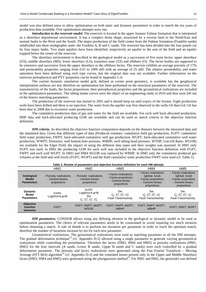
model was also defined anew to allow optimization on both static and dynamic parameters in order to match the ten years of production data available. Five optimization attempts were run.
Introduction to the reservoir model. The reservoir is located in the upper Jurassic Fulmar formation that is interpreted as a shoreface depositional environment. It has a complex dome shape, structured by a reverse fault to the North-East and normal faults to the West and the South. The major production of the field comes from the Fulmar formation (Franklin sands) subdivided into three stratigraphic units: the Franklin A, B and C sands. The reservoir has been divided into the four panels cut by four major faults. Two main aquifers have been identified, respectively an aquifer to the east of the field and an aquifer trapped below the centre of the reservoir.
The shoreface environment is described in the geological model as a succession of five main facies: upper shoreface (US), middle shoreface (MS), lower shoreface (LS), transition zone (TZ) and offshore (O). The facies bodies are supposed to be extensive and successive from the upper shoreface to the offshore facies. The reservoir exhibits an average porosity of 17% and permeability properties ranging from 0.01 to 1000 mD with an average of 25 mD. The relative permeability and water saturation have been defined using rock type curves, but the original data was not available. Further information on the reservoir petrophysical and PVT properties can be found in Appendix C-6.
The current dynamic simulation model grid, defined as corner point geometry, is available but the geophysical interpretation surfaces are not; therefore no optimization has been performed on the structural parameters of the reservoir. The transmissivity of the faults, the facies proportions, their petrophysical properties and the geostatistical realizations are included in the optimization parameters. The tubing intake curves were the object of an engineering study in 2010 and thus were left out of the history matching parameters.
The production of the reservoir has started in 2001 and it should keep on until expiry of the license. Eight production wells have been drilled and there is no injection. The water from the aquifer was first observed in the wells G6 then G4; G6 has been shut in 2008 due to excessive water production.
The cumulative production data of gas and water for the field are available. For each well back allocated production, BHP data and back-allocated producing GOR are available and can be used as match criteria in the objective function definition.
HM criteria. As described the objective function computation depends on the distance between the measured data and
the simulated data. Given that different types of data (Produced volumes: cumulative field gas production, FGPT; cumulative field water production, FWPT; back-allocated cumulative well gas production, WGPT; back-allocated cumulative well water production, WWPT; Pressures: well bottom hole pressure, WBHP; well tubing head pressure, WTHP; Gas-Oil Ratio: WGOR) are available for the Elgin Field, the impact of using the different data types and their weights was assessed. In HM1 only FGPT was used, in HM2 the producing GOR for each well was included in the objective function definition with FGPT, FWPT and each well WGPT. In HM3 and HM4 WGOR was replaced by WBHP. In HM5 only the cumulative produced gas volumes at the field and well levels (FGPT, WGPT) and the field cumulative water production FWPT were used (cf. Table 1).
Table 1: Review of parameters and objective function definition for each HM attempt
HM1 HM2 HM3 HM4 HM5
Geological Model
Parameters
- Porosity realizations - Cement lenses
proportions
- Porosity realizations - Cement lenses
proportions
- Facies realizations - Facies proportions
- Cement lenses proportions
- Facies realizations (global, local)
- Facies proportions - Cement lenses
proportions
- Facies realizations (global, local)
- Facies proportions - Cement lenses
proportions
Dynamic Model
Parameters Kz/Kh
Log(Kh)=A.φ+B
Kz/Kh Log(Kh)=A.φ+B
Swi 𝐿𝐿𝑟𝑟𝑟𝑟 , 𝐸𝐸𝑟𝑟
𝑟𝑟, 𝐸𝐸𝑟𝑟𝑤𝑤, 𝐸𝐸𝑤𝑤𝑟𝑟
Swi 𝐿𝐿𝑟𝑟𝑟𝑟 , 𝐸𝐸𝑟𝑟
𝑟𝑟, 𝐸𝐸𝑟𝑟𝑤𝑤, 𝐸𝐸𝑤𝑤𝑟𝑟 Fault Transmissivity
Swi 𝐿𝐿𝑟𝑟𝑟𝑟 , 𝐸𝐸𝑟𝑟
𝑟𝑟, 𝐸𝐸𝑟𝑟𝑤𝑤, 𝐸𝐸𝑤𝑤𝑟𝑟 Fault Transmissivity
Swi 𝐿𝐿𝑟𝑟𝑟𝑟 , 𝐸𝐸𝑟𝑟
𝑟𝑟, 𝐸𝐸𝑟𝑟𝑤𝑤, 𝐸𝐸𝑤𝑤𝑟𝑟 Fault Transmissivity
Objective function elements
FGPT FGPT, FWPT, WGPT, WGOR
FGPT, FWPT, WGPT, WBHP
FGPT, FWPT, WGPT, WBHP FGPT, FWPT, WGPT
HM parameters. CONDOR allows using any defining element in the geological or dynamic model to be used as optimization parameters. The choice of relevant parameters needs to be constrained to avoid requiring too much iteration before obtaining a match. A rule of thumb is to perform ten iterations per parameter in order to reach the optimum match, therefore the number of iterations increase by ten for each new parameter. Geostatistical realizations. The geostatistical realizations were used as matching parameter in all the HM attempts. The gradual deformation technique19 (cf. Appendix D-2) allowed using a single parameter to generate varying geostatistical realizations while controlling the perturbation. Therefore the facies (HM3, HM4 and HM5) or porosity realizations (HM1, HM2) for the four intervals (A sands, Lower B sands, Upper B sands and C sands) were each controlled by a gradual deformation parameter. The porosity and facies realizations were generated using the Fast Fourier Transform – Moving Average (FFT-MA) algorithm14 (cf. Appendix D-2) and the cemented lenses present only in the Upper and Middle Shoreface facies (HM3, HM4 and HM5) were generated using the plurigaussian method13. For HM1 and HM2, the geomodel was defined

How to Model Condensate Banking in a Simulation Model? Case Story of Elgin/Franklin 12
as a single facies with a decreasing trend in porosity along the Y axis and Z axis of the grid (Figure D-9), cemented lenses that have no permeability and no porosity were also modeled with a decreasing proportion trend along the Y axis. In HM3, HM4 and HM5 the geomodel was built on the distribution of the five facies of the shoreface environment with the inclusion of cemented lenses in the upper and lower shoreface facies. The petrophysical properties described in Appendix C-6 were respected.
Facies proportions. The cement lenses proportion were used as optimization parameters in all the history matching attempts and the proportion of Transition Zone and Lower Shoreface facies were used in HM3, HM4 and HM5 as regresseion parameters. The proportions were controlled using the facies proportions transformation option available in CONDOR (cf. Appendix D-2).
Permeability. In HM1 and HM2 the permeability was defined as a single permeability-porosity (log(K)=A.φ + B) relationship, the starting point is the result of the interpolation between the relationships defined by the operator for each layer/facies combination different quality; the A and B coefficients are used as optimization parameters. For HM3, HM4 and HM5 the log(K)=f(φ) relationships determined by the operator from core analysis performed were used (cf. Appendix C-6).
Relative permeability correlation (Lomeland, Ebeltoft and Thomas, 2005). In the absence of core data, the relative permeability tables have been used as optimization parameters in the HM process. The correlation chosen to perform the match is the LET correlation (cf. Appendix E), although any correlation can be implemented through the software. The chosen correlation allows giving convex/concave shapes to the relative permeability curve while keeping control of the entire range of saturation. The base case parameters were determined from the existing relative permeability tables available in the operator model. The parameters 𝐿𝐿𝑟𝑟𝑟𝑟 , 𝐸𝐸𝑟𝑟
𝑟𝑟, 𝐸𝐸𝑟𝑟𝑤𝑤 and 𝐸𝐸𝑤𝑤𝑟𝑟 were varied for the optimisation (cf. Table 2 and Figure 13). The other parameters were set as per the defined base case values. For HM4 and HM5 the same values of the Lomeland, Ebeltoft and Thomas (2005) correlation coefficients were used for all the tables.
Figure 13: Relative permeability range explored in the optimization (Gas-oil and Water oil
relative permeability Tables)
Table 2: Relative permeability optimization parameters
Parameter Base Case Min Max
𝑳𝑳𝒈𝒈𝒐𝒐 4.8 2 6
𝑬𝑬𝒐𝒐𝒈𝒈 2.6 0.5 4
𝑬𝑬𝒐𝒐𝒘𝒘 2 0.5 4
𝑬𝑬𝒘𝒘𝒐𝒐 2 0.7 4
Irreducible water saturation Swi. The value of the irreducible water saturation Swi, was used as optimization
parameter. It affects the initial water saturation distribution in the reservoir and the capillary pressure calculation. For HM2 and HM3 only one set of relative permeability table was used and therefore Swi was allowed to vary on a wide range from 0.05 to 0.45. In HM4 and HM5, five relative permeability tables were defined: one for each facies. Given that the porosity decreases from the upper shoreface facies to the offshore facies the value of Swi for each facies were defined as an offset from the value of Swi for the Upper Shoreface facies base on the rock type tables (cf. Appendix D-6). Therefore for HM4 and HM5 the value of Swi for the upper shoreface facies was used as optimization parameter (Swi was allowed to vary in the following range 0.03 to 0.15).
Fault transmissivity. For the HM1 and HM2 the fault transmissivity was left at a default value of 1. Adjusting the transmissivity of the Western Fault for instance can help reduce the water production markedly (cf. Figure C-11). For HM3, HM4 and HM5 they were introduced as history matching parameter based on the results of the previous sensitivity study that had been performed by GDF SUEZ E&P UK: the South East and East panel faults were set as non-leaking faults. The transmissivity of the East Panel aquifer, West Central panel, West panel faults and the fault between the G6 and G7 panels were introduced as a single optimization parameter (cf. Figure C-9 for the faults location and previously matched transmissivity values).
Results. HM1 (cf. Appendix D-3) optimization was performed to get familiarized with CONDOR interface. The
relative permeability definitions from the current GDF SUEZ E&P UK reservoir model with the associated relative permeability tables were used. HM1 illustrates the capacity of the algorithm to match a single vector of production data. The simulated FWPT perfectly fits the measured cumulative gas production. The optimum match was obtained in 89 iteration and a dozen of matched models have a close value for the objective function. However the other measured data do not fit so well the simulated production, for instance FWPT remains very different from the measured water production, highlighting a different behaviour of the matched model with the actual reservoir.

How to Model Condensate Banking in a Simulation Model? Case Story of Elgin/Franklin 13
HM2 (cf. Appendix D-4) was performed after trial runs were made to adjust the weight of the WGOR data serie in the objective function definition to match the contribution of WGPT. Initially the contribution of the GOR was overpowering the contributions of the other types of data. It can be observed that the contribution of the GOR towards the objective function did not change much throughout the iterations (Figure D-5) and did not seem to have a an impact on the optimization, a possible explanation is that the measured GOR data is noisy whereas the simulated GOR is very stable.
The quality of the match obtained with HM2 remains quite far from the measured production data. Even though some improvement is observed on the cumulative gas production compared to the initial model and a good agreement is visible in the early years of production, the quality of the results is not sufficient to validate the optimized models for forecasts. The well water production rate and the time of water breakthrough elude the match. Possibly the model as it is defined does not capture fully the dynamic flow behaviours of the real reservoir, also more emphasis could be given to matching the cumulative water production by increasing its weight in the objective function definition. It has also to be acknowledged that for this optimization, the simulation models considers all faults as leaking with a transmissibility factor of 1 (cf. Figure C-10 and Figure C-11). In the previous studies performed by GDF SUEZ E&P UK and the operator some major faults had been identified as flow boundaries (cf. Appendix C-7). The faults transmissibility should be included in the optimization parameters to solve this issue; this has been done from HM3 onwards.
A complementary method that can be implemented to improve the match for the different wells independantly is the local gradual deformations. Roggero, et al. (2007) used local gradual deformations to refine history matching in particular zones of the reservoir model. they observed that the method provides more flexibility in matching specific criteria in particular regions. Possible improvement on the match could also be obtained through increasing the number of chain iteration, but this would increase the total number of iterations accordingly.
The introduction of the WBHP data serie in the objective function definition for HM3 and HM4 did not help improve the efficiency of the convergence algorithm. The WBHP and FGPT data series are conflicting in the gradient calculation. Small changes in the model parameters resulted in big step changes (10% or more of the total objective function value) of the BHP contribution in the objective function, cancelling any smaller progress made on the match on gas or water production and making it difficult for the algorithm to assess properly the gradients for the calculation of the next iteration parameters (cf. Appendix D-5) in order to progress toward a good match on the FGPT and FWPT data series.
In HM5 only FGPT, FWPT and WGPT data series were left in the objective function definition with default weights. A small relative error (2%) was allowed for the FGPT data serie as it is measured at the separators and it is the primary target for history match. A relative error of 20% was allowed for WGPT data serie as it is the result of back allocation and 10 % for the FWPT data serie. It can be observed that the FWPT data serie is the main target of the optimization algorithm throughout the iterations (cf. Figure 14). This is possibly explained by the great relative distance of the simulated data to the measured data (cf. Appendix D-7) and highlights the algorithm focus on the most efficient way to reduce the total value of the objective function. The next step would have been to match the contribution of the FWPT and FGPT data series in the first iteration to assess how the optimization progresses but not enough time was available.
Figure 14: Objective function contribution of the different
production data in HM 5 HM5 did not lead to a satisfying match as the optimization process focused its energy to the minimization of the
simulated values for FWPT which still remained twice as much as the measured data after 122 iterations. No progress was made during the optimization to improve the match on the FGPT data serie (cf. Appendix D-7).
Discussion. CONDOR is a powerful tool for assisted history matching, the possibilities for parameterization of the geological and dynamic models are extensive, however the choice of parameters and production data used to calculate the objective function should be made wisely. Attention must also be paid to the selection of the weights and the relative errors allowed for the data. Trying to match for instance both BHP and cumulative gas and water production proved problematic for the Elgin field. The choice of the weights affects the way the software manage the optimization. If a production data has a too important contribution to the objective function total value, the algorithm will focus on reducing its contribution neglecting the less contributing elements that may be of primary importance to the match.
The freedom to define the geological models and the parameters is definitely an asset of the software. However if one wants to respects the geological model as described by the Geophysics and Geology team and with the petrophysical information extracted from the core analysis, this freedom can become overwhelming as the parameters become too numerous and cannot all be regressed upon. It then becomes critical to identify which parameters will be the most suited to be the object of the optimization. As seen here in HM1 and HM2 the reservoir permeability could be modified directly through changing the
How to Model Condensate Banking in a Simulation Model? Case Story of Elgin/Franklin 14
parameters of the function log(Kh)=f(φ). In HM3, HM4 and HM5 the field permeability was controlled indirectly by changing the facies proportions. It would have been too demanding of computing power to try to control the thirteen log(Kh)=f(φ) relationships defined for each facies – interval combination, this would have resulted in 24 supplementary optimization parameters, hence 240 supplementary iterations.
Finally consideration to computing power necessary must be given, the original simulation model required 3.5 hours to be run. After simplification of the model and the schedule, the simulation time was reduced to 30 minutes. The great number of iterations implies leaving the optimization run for a week before obtaining the optimised result. The choice of the weights and the optimization parameters is thus critical to ensure efficiency. Conclusions A review of the existing relative gas-condensate permeability models implemented in the commercial reservoir simulator ECLIPSE has been achieved. The impact of condensate banking in the Elgin Field has been studied using these models on single well and full field reservoir models.
The pseudopressure well productivity computation proved to be a useful tool to account for capillary number dependent relative permeability in the full field model, removing the need for local grid refinement and keeping the simulation time close the original model simulation time. The fine grid simulation results when using the Henderson capillary number modified relative permeability model were matched on the coarse grid single well model when using the GPP option with Capillary number dependant relative permeabilities.
The single well model results have shown that the impact of condensate banking on productivity in the Elgin Field should be small and less than the uncertainty on the back allocated production rates as already shown by Mott in 2006.
Sensitivity has been demonstrated to the Henderson model parameters relating the CN-dependent oil relative permeability and those should be the focus of an accurate determination.
The use of the gas-condensate relative permeability is required to accurately capture the condensation effects on productivity in the full field simulation model but further work specific to the Elgin Field should be done.
A study of how to achieve history matching of the Elgin Field using the software CONDOR has been performed. A great sensitivity to the choice of matching parameters and the objective function function definition has been shown.
No satisfying history matched model was obtained despite the great number of simulation iterations performed. A seemingly way to reach the desired match objective would be to outweigh the objective function contribution of FGPT and give a secondary place to the other matching criteria. Trying to include all the production data with the same weight did not lead to satisfying results and should be done carefully. Further Work Further simulation of the full field model of the Elgin field need to be performed to investigate further the grid size required to accurately model the Capillary number dependant relative permeability effects in combination with the pseudopressure computation.
The characterization of condensate banking effects in the Elgin field should be studied further with the accurate determination of velocity dependent relative permeability parameters through pseudosteady state laboratory experiments and acquisition of well test data. This would allow a more precise understanding and modelling of the physical phenomenon occurring in the near wellbore region for the Elgin field. If independent well production data was to be acquired the condensate banking model parameters could also be adjusted through history matching.
The quality of the reservoir model HM could be improved with the addition of well observation data in the geomodel definition and the HM could be generalized further with the introduction of the structural model in the HM parameters. Also the number of chained iterations (introduction of new seeds in the gradual deformations) could be increased to explore further uncertainty space for the geostatistical realizations. Last, the way to go seems to be to increase the use of local gradual deformations and facies proportions fitting to reach a satisfying match while using proper weights when a lot of data series are available.
Finally the Bayesian framework combining the use of CONDOR and COUGAR could be implemented to obtain probabilistic production forecasts for the Elgin Field with the implementation of the model for condensate banking effects. Nomenclature C = gas rate constant 𝑑𝑑𝑗𝑗 = observation data vector, j=1,…,m D = depth, m 𝑓𝑓𝑗𝑗(𝛼𝛼) = simulated data vector and 𝛼𝛼 is the uncertain parameter, j=1,…,m FPR = field pressure, bars h = reservoir thickness, m HPHT = high pressure - high temperature
𝑘𝑘�⃗�⃗ = permeability tensor kr = relative permeability, fraction 𝑘𝑘𝑟𝑟∗ = end-point relative permeability, fraction

How to Model Condensate Banking in a Simulation Model? Case Story of Elgin/Franklin 15
𝑘𝑘𝑟𝑟𝑟𝑟𝑟𝑟 = capillary number modified relative permeability of the pth phase K = absolute permeability, md Kh = horizontal permeability, md Kz = vertical permeability, md m = number of observations M = molecular weight, g/mol 𝑁𝑁𝑐𝑐 = capillary number Ncbp = phase base Capillary Number Ncnp = normalized Capillary Number p = pressure, bars p* = pressure at outer boundary of region 1, bars pd =dew point pressure, bars ∆𝑝𝑝𝑟𝑟 = total pseudopressure pr = average reservoir pressure, bars pwf =wellbore flowing pressure, bars ∆𝑃𝑃𝑟𝑟 = pressure drop of the pth phase in the direction of flow, bars q = flow rate, sm3/day R = gas constant re = external drainage radius, m rw = wellbore radius, m s = skin factor S = saturation, fraction S* = normalised or HCPV saturation, fraction 𝑆𝑆𝑟𝑟 = residual saturation, fraction T = reservoir temperature, ºC 𝑣𝑣 = velocity in the direction of flow, m/s wj = jth weight of the objective function α = inversion parameter βs = surface gas mole fraction in wellstream, fraction 𝜀𝜀 = Corey exponent for the curvature of the permeability function φ = porosity, fraction 𝜵𝜵��⃗ 𝜱𝜱 = flow potential gradient ρ = density, kg/m3 𝜎𝜎 = gas-oil surface tension, mN/m Subscripts g = gas i = irreducible I = immiscible M = miscible o = oil p = phase indicator sc = standard conditions w = water References 1. Ayyalasomayajula, P., N. Silpngarmlers, and J. Kamath. “Well Deliverability Predictions for a Low-Permeability Gas/Condensate
Reservoir.” paper SPE 95529, prepared for presentation at the SPE Annual Technical Conference and Exhibition held in Dallas, Texas, USA, 9-12 October, 2005.
2. Bang, V., V. Kumar, P.S. Ayyalasomayajula, G.A. Pope, and M.M. Sharma. “Relative Permeability of Gas-Condensate Fluids: A General Correlation.” paper SPE 102741, prepared for presentation at the SPE Annual Technical Conference and Exhibition held in San Antonio, Texas, USA, 24-27 September, 2006.
3. Blom, S. M.P., and J. Hagoort. “The Combined Effect of Near-Critical Relative Permeability and Non-Darcy Flow on Well Impairment by Condensate Drop Out.” paper SPE 51367, first presented at the SPE Gas Technology Symposium, Calgary, Canada, 16-18 March, 1998.
4. Blom, S.M.P., and J. Hagoort. “How to Include the Capillary Number in Gas Condensate Relative Permeability Functions?” paper SPE 49268, prepared for presentation at the SPE Annual Technical Conference and Exhibition held in New Orleans, Louisiana, USA, 27-30 September, 1998.
5. Busby, D. and Feraille, M.: “Adaptive Design of Experiments for Bayesian Inversion – An Application to Uncertainty Quantification of a Mature Oil Field,” presented at 6th International Conference on Inverse Problems in Engineering: Theory and Practice, 15-19 June 2008 Dourdan (Paris) France, Journal of Physics: Conference Series vol. 135, No.012026.
6. Delshad, M., D. Bhuyan, G.A. Pope, and L.W. Lake. “Effect of Capillary Number on the Residual Saturation of a Three-Phase Micellar Solution.” Paper SPE 14911, prepared for presentation at the SPE Enhanced Oil Recovery Symposium, held in Tulsa, Oklahoma, USA, 20-23 April, 1986.

How to Model Condensate Banking in a Simulation Model? Case Story of Elgin/Franklin 16
7. Fevang, Ø., and C.H. Whitson. “Modelling Gas Condensate Well Deliverability.” paper SPE 30714, presented at the SPE Annual Technical Conference and Exhibition held in Dallas, USA, 22-25 October, 1995.
8. Henderson, G.D., A. Danesh, D.H. Tehrani, and B. Al-Kharusi. “The Relative Significance of Positive Coupling and Inertial Effects on Gas Condensate Relative Permeabilities at High Velocity.” paper SPE 62933, presented at the SPE Annual Technical Conference and Exhibition held in Dallas, Texas, USA, 1-4 October, 2000.
9. Gringarten, A. C., O. Oregunwo, and G. Uxukbayev. “Assessment of Rate-Dependent Skin Factors in Gas Condensate and Volatile Oil Wells.” paper SPE 143592, prepared for presentation at the 2011 SPE EUROPEC/EAGE Annual Conference and Exhibition held in Vienna, Austria, 23-26 May, 2011.
10. IFP Energies Nouvelles. Condor research prototype software documentation - Version 2.6. User guide. 2011. 11. Jamiolahmady, M., A. Danesh, G. Henderson, and G.D. Tehrani. “Variations of Gas-Condensate Relative Permeability with Production
Rate at Near Wellbore Conditions: A General Correlation.” paper SPE 83960, prepared for presentation at Offshore Europe 2003 held in Aberdeen, UK, 2-5 September, 2003.
12. Kamath, J.. “Deliverability of Gas-Condensate Reservoirs – Field Experiences and Prediction Techniques.” JPT vol. 59, no. 4 (April 2007): 94-99.
13. Le Loc'h, G., and A. Galli. “Truncated plurigaussian method: theoretical and practical points of view.” Edited by E.Y. Baafi and N.A. Schofield. Wollongong'96 (Kluwer Academic Press), 1997: 211-222.
14. Le Ravalec, M., B. Noetinger, and L-Y. Hu. “The FFT moving average (FFT-MA) generator: An efficient tool for generating and conditioning.” Mathematical Geology 32, no. 6 (2000): 701-723.
15. Lomeland, F., E. Ebeltoft, and W.H. Thomas. “A New Versatile Relative Permeability Correlation.” paper SCA2005-32 presented at the International Symposium of the Society of Core Analysts held in Toronto,Canada, 21-25 August, 2005.
16. Mott, R.E. “Engineering Calculations of Gas-Condensate-Well Productivity.” paper SPE 86298 (2003), first presented at the SPE Annual Technical Conference and Exhibition held in San Antonio, Texas, USA, 29 September-2 October, 2002.
17. Oliver, D.S., and Y. Chen. “Recent Progress on Reservoir History Matching: a Review.” Computational Geosciences (Springer Netherlands) Vol. 15, no. 1 (2011):185-221
18. Pope, G.A., W. Wu, G. Narayanaswamy, M. Delshad, M.M. Sharma, and P. Wang. “Modelling Relative Permeability Effects in Gas-Condensate Reservoirs With A New Trapping Model.” paper SPE 62497 (2000), first presented at the SPE Annual Technical Conference and Exhibition, New Orleans, Louisiana, USA, 27-30 September, 1998.
19. Roggero, F. and Hu., L.Y.:”Gradual Deformation of Continuous Geostatistical Models for History Matching,” paper SPE 49004 presented at the SPE Annual Technical Conference and Exhibition, New Orleans, Louisiana, Sept. 27-30, 1998.
20. Roggero, F., D-Y. Ying, P.H. Berthet, O. Lerat, J. Cap, and P.E. Schreiber. “Macthing of Production History and 4D Seismic Data - Application to the Girassol Field, Offshore Angola.” paper SPE 109929, prepared for presentation at the SPE Annual Technical Conference and Exhibition held in Anaheim, California, USA, 11-14 November, 2007.
21. Schlumberger. ECLIPSE Technical Description (2009.2). 22. Schaaf, T., B. Coureaud, N. Labat, and D. Busby. “Using Experimental Designs, Assisted History-Matching Tools, and Bayesian
Framework to Get Probabilistic Gas-Storage Pressure Forecasts.” paper SPE 113498 (2009), presented at the EUROPEC/EAGE Conference and Exhibition held in Rome, Italy, 9-12 June, 2008.
23. Singh, K., and C. H. Whitson. “Gas-Condensate Pseudopressure in Layered Reservoirs.” paper SPE 117930, presented at the Abu Dhabi International Petroleum Exhibition and Conference held in Abu Dhabi, UAE, 3-6 November 2008, 2008.
24. Vizika, O., and F. Kalaydjian. “Effect of Capillary, Viscous and Gravity Forces on Gas Condensate Mobility.” paper SCA2002-24, 2002.
25. Whitson, C. H., and Ø. Fevang. “Gas Condensate Relative Permeabilities for Well Calculations.” paper SPE 56476, prepared for presentation at the 1999 SPE Annual Technical Conference and Exhibition held in Houston, Texas, USA, 3-6 October, 1999.
26. Xiao, J.J., and A.J. Al-Muraikhi. “A New Method for the Determination of Gas Condensate Well Production Performance.” paper SPE 90290, prepared for presentation at the SPE Annual Technical Conference and Exhibition held in Houston, Texas, USA, 26-29 September, 2004.
27. Yuan, C., and G.A. Pope. “A New Method to Model Relative Permeability in Compositional Simulators to Avoid Discontinuous Changes Caused by Phase Identification Problems.” paper SPE 142093, prepared for presentation at the SPE Reservoir Simulation Symposium held in the Woodlands, Texas, USA, 21-23 February, 2011.

How to Model Condensate Banking in a Simulation Model? Case Story of Elgin/Franklin 17
Appendix
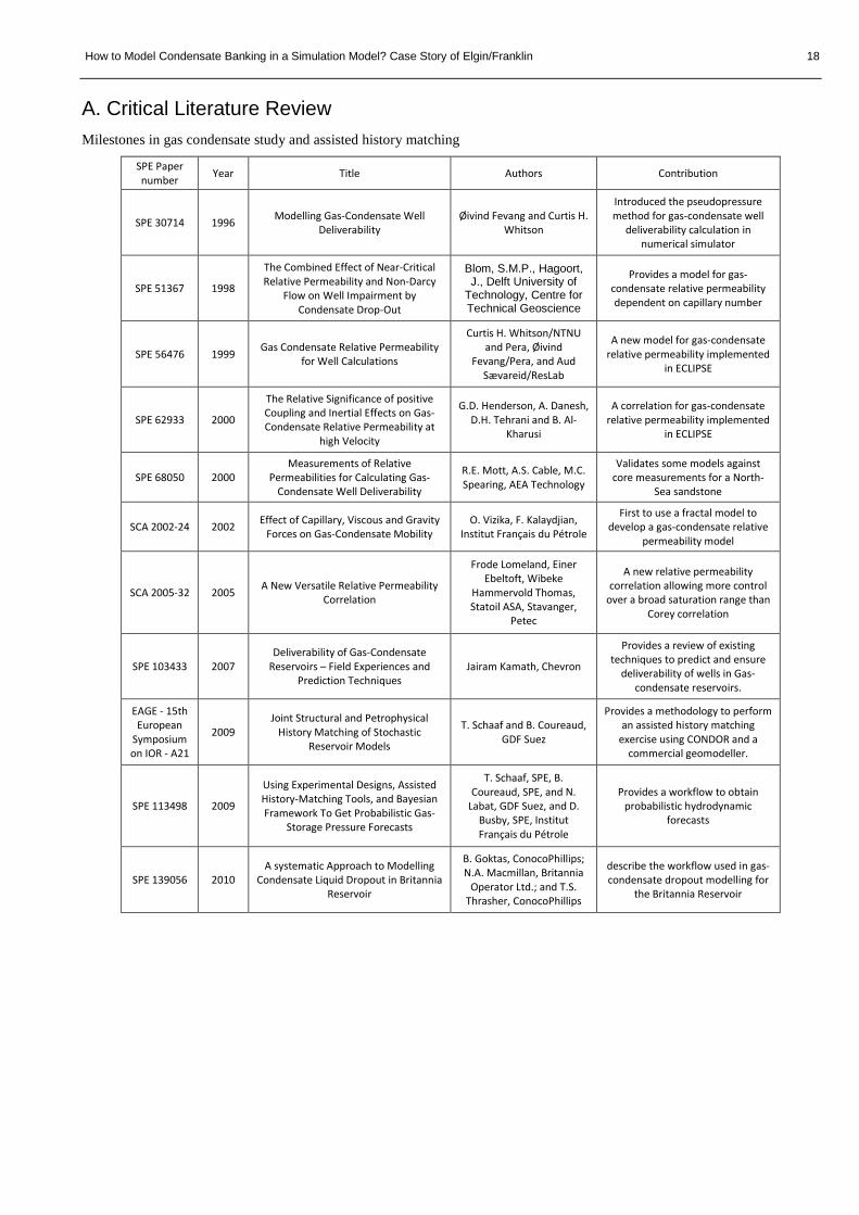
How to Model Condensate Banking in a Simulation Model? Case Story of Elgin/Franklin 18
A. Critical Literature Review Milestones in gas condensate study and assisted history matching
SPE Paper number Year Title Authors Contribution
SPE 30714 1996 Modelling Gas-Condensate Well Deliverability
Øivind Fevang and Curtis H. Whitson
Introduced the pseudopressure method for gas-condensate well
deliverability calculation in numerical simulator
SPE 51367 1998
The Combined Effect of Near-Critical Relative Permeability and Non-Darcy
Flow on Well Impairment by Condensate Drop-Out
Blom, S.M.P., Hagoort, J., Delft University of
Technology, Centre for Technical Geoscience
Provides a model for gas-condensate relative permeability dependent on capillary number
SPE 56476 1999 Gas Condensate Relative Permeability for Well Calculations
Curtis H. Whitson/NTNU and Pera, Øivind
Fevang/Pera, and Aud Sævareid/ResLab
A new model for gas-condensate relative permeability implemented
in ECLIPSE
SPE 62933 2000
The Relative Significance of positive Coupling and Inertial Effects on Gas-Condensate Relative Permeability at
high Velocity
G.D. Henderson, A. Danesh, D.H. Tehrani and B. Al-
Kharusi
A correlation for gas-condensate relative permeability implemented
in ECLIPSE
SPE 68050 2000 Measurements of Relative
Permeabilities for Calculating Gas-Condensate Well Deliverability
R.E. Mott, A.S. Cable, M.C. Spearing, AEA Technology
Validates some models against core measurements for a North-
Sea sandstone
SCA 2002-24 2002 Effect of Capillary, Viscous and Gravity Forces on Gas-Condensate Mobility
O. Vizika, F. Kalaydjian, Institut Français du Pétrole
First to use a fractal model to develop a gas-condensate relative
permeability model
SCA 2005-32 2005 A New Versatile Relative Permeability Correlation
Frode Lomeland, Einer Ebeltoft, Wibeke
Hammervold Thomas, Statoil ASA, Stavanger,
Petec
A new relative permeability correlation allowing more control
over a broad saturation range than Corey correlation
SPE 103433 2007 Deliverability of Gas-Condensate
Reservoirs – Field Experiences and Prediction Techniques
Jairam Kamath, Chevron
Provides a review of existing techniques to predict and ensure
deliverability of wells in Gas-condensate reservoirs.
EAGE - 15th European
Symposium on IOR - A21
2009 Joint Structural and Petrophysical
History Matching of Stochastic Reservoir Models
T. Schaaf and B. Coureaud, GDF Suez
Provides a methodology to perform an assisted history matching
exercise using CONDOR and a commercial geomodeller.
SPE 113498 2009
Using Experimental Designs, Assisted History-Matching Tools, and Bayesian Framework To Get Probabilistic Gas-
Storage Pressure Forecasts
T. Schaaf, SPE, B. Coureaud, SPE, and N.
Labat, GDF Suez, and D. Busby, SPE, Institut Français du Pétrole
Provides a workflow to obtain probabilistic hydrodynamic
forecasts
SPE 139056 2010 A systematic Approach to Modelling
Condensate Liquid Dropout in Britannia Reservoir
B. Goktas, ConocoPhillips; N.A. Macmillan, Britannia
Operator Ltd.; and T.S. Thrasher, ConocoPhillips
describe the workflow used in gas-condensate dropout modelling for
the Britannia Reservoir

How to Model Condensate Banking in a Simulation Model? Case Story of Elgin/Franklin 19
SPE 30714-PA (1996)
Modelling Gas-Condensate Well Deliverability
Authors: Øivind Fevang and Curtis H. Whitson
Contribution to the understanding of Gas-Condensate reservoir modelling:
Introduced a pseudopressure method to model gas-condensate well deliverability in reservoir simulators.
Objectives of the paper:
To introduce and accurate method for modelling the deliverability of gas-condensate wells.
Methodology used:
- Developed a method to get pressures and saturations easily from the producing GOR.
- Compared fine grid and coarse grid simulation.
- Checked the influence of different parameters on gas-condensate well deliverability (Interfacial tension, critical oil
saturation)
Conclusions reached:
- Gas-condensate wells producing with BHFP lower than the dew point have up to three flow regions. Region 1 has a
constant flowing composition (GOR) where both gas and oil flow simultaneously. Most of the deliverability loss is
caused by reduced gas permeability in Region 1. Region 2 is where condensate accumulates but has no mobility.
Region 3 is the outer region where reservoir pressure is greater than the dew point and only gas flows.
- Provided a simple method for calculating bottom hole flowing pressure in coarse grid models.
- The multiphase pseudopressure function is calculated in three parts, based on three flow regions.
- Local grid refinement is not needed for gas-condensate wells in full field model.
- Critical oil saturation has no effect on gas-condensate well deliverability

How to Model Condensate Banking in a Simulation Model? Case Story of Elgin/Franklin 20
SPE 51367 (1998)
The combined effect of Near-Critical Relative Permeability and Non-Darcy Flow on Well Impairment by Condensate Drop
Out
Authors: Saskia M.P. Blom and Jacques Hagoort
Contribution to the understanding of Gas-condensate relative permeability modelling:
Introduces a comprehensive numerical method to calculate well impairment based on steady-state radial flow. The method
incorporates near-critical relative permeability and saturation-dependent inertial resistance.
Objectives of the paper:
To present a calculation method for the evaluation of the combined effect of near-critical two-phase flow and high velocity
flow on well impairment by condensate drop-out. To demonstrate the significance of these combined effects. To demonstrate
the significance of the use of proper relative permeability curves for the estimation of well impairment caused by condensate
drop-out.
Methodology used:
Represent relative permeability functions by a Corey function with coefficients dependent on the capillary number. The Corey
coefficients are interpolated between their capillary dominated (immiscible) limits and their viscous dominated (miscible
limits). The interpolation is affected by a weighting function dependent on the capillary number.
Conclusion reached:
- Extended the steady-state method for the calculation of well impairment by condensate drop-out to account for both
near-critical relative permeability and non-Darcy flow.
- Condensate drop-out aggravates the inertial pressure losses (non-Darcy flow).
- Near-critical relative permeability and inertial resistance are strongly coupled.
- A simple superposition of the separate effects may significantly underestimate the well impairment.
- The use of proper near-critical relative permeability curves is all the more important if non-Darcy flow is significant.
- Well Impairment by condensate drop-out may be grossly overestimated if the dependence on relative permeability on
the capillary number is ignored.
Comments:
Requires experimental data to determine parameters
SPE 56476 (1999)
Gas Condensate Relative Permeability for Well Calculations
Authors: Curtis H. Whitson, Øivind Fevang and Aud Sævareid
Contribution to the understanding of Gas-condensate reservoir modelling:
Proposed a model for krg = f(krg/kro) including the effect of capillary number.
Objectives of the paper:
To present an engineering approach to treating gas-oil relative permeabilities describing near-well flow in gas condensate
wells. To conduct an experimental program to develop an apparatus suitable for measuring steady-state gas-oil relative
permeabilities for synthetic model and reservoir fluid systems and study the effects of varying flow conditions in a gas
condensate well. To correlate measured relative permeability data using a generalized equation that consists of a traditional

How to Model Condensate Banking in a Simulation Model? Case Story of Elgin/Franklin 21
“immiscible” Corey-Type relation and a simple one-parameter correlation for capillary number dependence.
Methodology used:
The approach is founded on the fundamental flow behavior near and around gas condensate wells. It involves an experimental
program and a modelling program to correlate measured relative permeability data.
Conclusions reached:
- The oil saturation history experienced in the near-well region of a gas condensate well consists of an unlimited
number of cycles of complete or partial drainage and imbibition. The effect of saturation hysteresis is minimal on the
fundamental relative permeability relation krg = f(krg/kro) .
- A relative permeability model is proposed for fitting steady-state gas/oil relative permeability behaviour, including the
effect of capillary number on krg = f(krg/kro).
- The effect of capillary number on gas/oil relative permeability can result in a significant improvement in gas relative
permeability and thereby reduce the negative impact of condensate blockage.
- An approach is given for incorporating the improvement in krg at high capillary numbers, and the detrimental effect of
inertial high velocity flow (“turbulence”) as part of the two-phase condensate pseudopressure model. The key to this
approach is estimating velocity as a function of pressure in the reservoir using an appropriate form of Darcy’s law for
the well-flow geometry.

How to Model Condensate Banking in a Simulation Model? Case Story of Elgin/Franklin 22
SPE 62933 (2000)
The relative significance of positive coupling and inertial effects on gas condensate relative permeabilities at high velocity.
Authors: G.D. Henderson, A. Danesh, D.H. Tehrani and B. Al-Kharusi
Contribution to the understanding of relative permeability modelling:
Highlighted the effects of positive coupling on gas-condensate wells productivity.
Objectives of the paper:
To investigate the flow of gas-condensate fluids in the wellbore region of gas condensate reservoirs, and in particular to
investigate the effect that inertia would have on relative permeability. To develop empirical correlations which relate the
change if gas-condensate relative permeability to variations in fluid saturation, velocity and interfacial tension.
Methodology used:
Used the acquisition of experimental data at different velocity, saturations and over a range of interfacial tension for
condensing fluids to investigate the positive coupling effects.
Conclusion reached:
- The effects of positive coupling were evident at high velocity and at high interfacial tension for three different cores,
with the gas relative permeability increasing with increasing velocity at near wellbore flow rates
- Described the flow behaviour estimating the combined effects of coupling of gas and condensate phases (positive) and
inertial losses (negative) and proposed two separate mathematical expressions to determine them.

How to Model Condensate Banking in a Simulation Model? Case Story of Elgin/Franklin 23
SPE 68050 (2000)
Measurements of Relative Permeabilities for Calculating Gas-Condensate Well Deliverability
Authors: R.E. Mott, A.S. Cable, M.C. Spearing, AEA Technology
Contribution to the understanding of Gas-condensate reservoir modelling:
The paper shows the clear increase in mobility with capillary number and describes how the data can be modeled with
empirical correlations which can be used in reservoir simulators.
Objective of the paper:
Perform relative permeability measurements on a sandstone core from a North Sea gas-condensate reservoir, at velocities that
are typical of the near-well region.
Methodology used:
The following experimental techniques were used: Constant Volume Depletion (CVD) coreflood experiment on a reservoir
fluid sample; Steady-state technique; PseudoSteady-State Method.
Conclusions reached:
- Observed different behaviour in low-rate, depletion experiments and the high-rate, pseudosteady-state experiments.
- The results suggest that the models assuming capillary number as single parameter to account for both the effects of
flow rate and interfacial tensions may not be valid for flows at low rate and low IFT (happening in the deep reservoir
zone at high pressure).
- Any reduction in mobility caused by inertial flow is less important than the increase due to high capillary number.
- High rate relative permeability measurements on a North Sea sandstone core show a significant increase in relative
permeability with capillary number.
- Gas relative permeability measurement results showed no rate dependency, but there was evidence for an increase in
relative permeability due to low IFT.
Comments:
This paper shows a correlation with acceptable results compared to experiments on a North Sea sandstone core.

How to Model Condensate Banking in a Simulation Model? Case Story of Elgin/Franklin 24
SCA 2002-24 (2002)
Effect of Capillary, Viscous and Gravity Forces on Gas-Condensate Mobility
Authors: O. Vizika, F. Kalaydjian, Institut Français du Pétrole
Contribution to the understanding of gas-condensate banking modelling:
Offers a different way of modelling the flow of gas-condensate in the reservoir.
Objective of the paper:
To present a model for gas condensate Kr as a function of the capillary number and to demonstrate that apparently
contradictory laboratory results on the dependence on interfacial tension and flow rate, separately considered, can be
reconciled. Also a modelling of the combined effect of gravity and capillary forces on the critical condensate saturation is
introduced.
Methodology used:
Modelling method based on the fractal filling of a fractal structure by a wetting fluid, deGennes (1995). The relationships
described use the capillary number proposed by Dullien (1992)
Conclusion reached:
- A model to calculate gas condensate Kr as functions of the capillary number has been proposed. The model includes
the structure characteristics of the porous medium through its fractal dimension. The model has been tested against
experimental results reported in the literature and a very satisfying agreement has been obtained.
- A threshold condensate saturation, Stc, can be predicted below which the condensate mobility is extremely reduced,
even though finite.
- The critical saturation for condensate mobility, Scc, increases with increasing interfacial tension (decreasing Bond
number) and fractal dimension.
Comments:
Applicable method that will require guessing of finding the parameter DL.
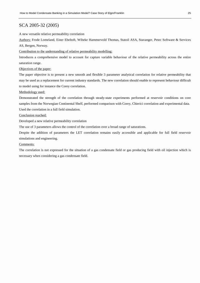
How to Model Condensate Banking in a Simulation Model? Case Story of Elgin/Franklin 25
SCA 2005-32 (2005)
A new versatile relative permeability correlation Authors: Frode Lomeland, Einer Ebeltoft, Wibeke Hammervold Thomas, Statoil ASA, Stavanger, Petec Software & Services
AS, Bergen, Norway.
Contribution to the understanding of relative permeability modelling:
Introduces a comprehensive model to account for capture variable behaviour of the relative permeability across the entire
saturation range.
Objectives of the paper:
The paper objective is to present a new smooth and flexible 3 parameter analytical correlation for relative permeability that
may be used as a replacement for current industry standards. The new correlation should enable to represent behaviour difficult
to model using for instance the Corey correlation.
Methodology used:
Demonstrated the strength of the correlation through steady-state experiments performed at reservoir conditions on core
samples from the Norwegian Continental Shelf, performed comparison with Corey, Chierici correlation and experimental data.
Used the correlation in a full field simulation.
Conclusion reached:
Developed a new relative permeability correlation
The use of 3 parameters allows the control of the correlation over a broad range of saturations.
Despite the addition of parameters the LET correlation remains easily accessible and applicable for full field reservoir
simulations and engineering.
Comments:
The correlation is not expressed for the situation of a gas condensate field or gas producing field with oil injection which is
necessary when considering a gas condensate field.

How to Model Condensate Banking in a Simulation Model? Case Story of Elgin/Franklin 26
SPE 103433-MS (2007)
Deliverability of Gas-Condensate Reservoirs – Field Experiences and Prediction Techniques
Authors: Jairam Kamath, Chevron
Contribution to the understanding of Gas-condensate banking modelling:
Provides a review of existing techniques to predict and ensure deliverability of wells in Gas-condensate reservoirs.
Objective of the paper:
To outline the five steps to predict deliverability loss caused by condensate banking; to discuss integrated laboratory/simulation
field studies used to validate these steps and to explore options to improve well deliverability.
Methodology used:
Extensive review of technical papers on gas condensate reservoir deliverability.
Conclusion reached:
Highlight the need of a five-step approach (appropriate laboratory measurements, fitting laboratory data to relative
permeability models, use of spreadsheet tools, single-well models and full field models) to predict deliverability loss caused by
condensate banking reasonably.
Emphasize the need for further testing of existing relative permeability models and further work on productivity improvement
by fracturing and chemical treatments.
Comments:
Underlines the steps to follow to conduct a proper study of deliverability loss for gas-condensate reservoirs; resumes the
necessary data required to conduct the study and the possible methods to use.

How to Model Condensate Banking in a Simulation Model? Case Story of Elgin/Franklin 27
EAGE - 15th European Symposium on Improved Oil Recovery - A21 (2009) Joint Structural and Petrophysical History Matching of Stochastic Reservoir Models
Authors: T. Schaaf and B. Coureaud, GDF Suez
Contribution to the understanding of History Matching:
Demonstrated the use of a history matching method tackling simultaneously structural, petrophysical and fluid related
parameters in a synthetic reservoir application.
Objectives of the paper:
Find a way to capitalize on reviewed existing models to perform a joint structural and petrophysical history matching.
Methodology used:
Joint geological and simulation model updating using assisted history matching software (CONDOR Research Prototype 2008)
and a geomodelling software with internal workflow (PETREL RE).
Conclusion reached:
The history matching method proposed shows promising results
Comments:
Provides a methodology to perform an assisted history matching exercise using CONDOR Research Prototype 2008.

How to Model Condensate Banking in a Simulation Model? Case Story of Elgin/Franklin 28
SPE 113498 (2009) Using Experimental Designs, Assisted History-Matching Tools, and Bayesian Framework To Get Probabilistic Gas-Storage
Pressure Forecasts
Authors: T. Schaaf, SPE, B. Coureaud, SPE, and N. Labat, GDF Suez, and D. Busby, SPE, Institut Français du Pétrole
Contribution to the understanding of History-Matching and Production Forecast:
Described the workflow to obtain multiple history-matched models and to perform combined Bayesian inversion applied to a
gas storage reservoir.
Objectives of the paper:
The objective is to propose a workflow combining different methods to integrate and reduce most of the subsurface
uncertainties using multiple history-matched models to infer reasonably reliable forecasts of gas-storage pressure.
Methodology used:
- Perform a sensitivity study to retain the most sensitive static and dynamic uncertainties
- Use assisted history-matching tools to obtain multiple history-matched models
- Combine multiple history-matched models with the uncertain parameters not retained in the sensitivity study to obtain
probabilistic pressure profiles.
- Use Bayesian framework to constrain uncertain parameters with observation data
Conclusion reached:
A new workflow to obtain hydrodynamics forecasts has been set up. It can be described in the following steps:
- Experimental design techniques are used to conduct both structural and petrophysical sensitivity studies as a pre-
processor step of the history matching process.
- Retaining only the most sensitive parameters, multiple history-matched models are obtained using a versatile history
matching software
- Using the history matched models in a joint modelling method, uncertainties are propagated and probabilistic
forecasts are obtained.
Comments:
Provides a workflow to obtain probabilistic hydrodynamic forecasts

How to Model Condensate Banking in a Simulation Model? Case Story of Elgin/Franklin 29
SPE 139056 (2010)
A systematic Approach to Modelling Condensate Liquid Dropout in Britannia Reservoir
Authors: B. Goktas, ConocoPhillips; N.A. Macmillan, Britannia Operator Ltd.; and T.S. Thrasher, ConocoPhillips
Contribution to the understanding of Gas-Condensate banking modelling:
Demonstrates a systematic and comprehensive production data analysis approach for modelling well productivity decline due
to condensate liquid dropout with field examples.
Objectives of the paper:
To describe the workflow used in gas-condensate dropout modelling for the Britannia Reservoir
Methodology used:
- Construction of back-pressure well deliverability plots
- Analysis of back-pressure deliverability plots
- Sector modelling
Conclusions reached:
- Back-pressure well deliverability plots are instrumental in monitoring performances of gas condensate wells
- Well deliverability plots can be used as a guide for producing pseudo relative permeability curves
Comments:
Compares local grid refinement and Coarse Grid model using pseudopressure computation solution.
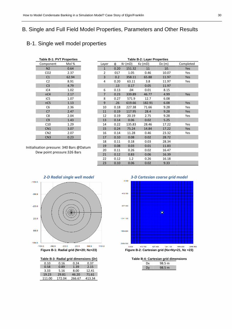
How to Model Condensate Banking in a Simulation Model? Case Story of Elgin/Franklin 30
B. Single and Full Field Model Properties, Parameters and Other Results
B-1. Single well model properties
Table B-1: PVT Properties Component Mol %
N2 0.64 CO2 2.37 C1 62.94 C2 8.91 C3 4.79 iC4 1.02 nC4 2.17 iC5 1.07 nC5 1.13 C6 2.36 C7 2.47 C8 2.04 C9 1.43
C10 1.29 CN1 3.07 CN2 2.07 CN3 0.23
Initialisation pressure: 340 Bars @Datum
Dew point pressure:326 Bars
Table B-2: Layer Properties Layer φ Kr (mD) Kz (mD) Dz (m) Completed
1 0.20 151.32 11 10. Yes 2 0 17 1.05 0.46 10.07 Yes 3 0.2 358.11 65.88 11.97 Yes 4 0.20 63.11 3.8 11.97 Yes
.13 0.17 0.05 11.97 6 0.13 .04 0.01 8.15 7 0.23 339.89 46.77 4.99 Yes 8 0.27 571.9 12.7 6.08 9 .26 619.66 182.91 6.08 Yes
10 0.18 227.38 71.66 9.28 Yes 11 0.19 117.95 28.4 9.28 Yes 12 0.19 20.19 2.75 9.28 Yes 13 0.14 0.06 0.02 5.25 14 0.22 135.83 28.46 17.22 Yes 15 0.24 75.24 14.84 17.22 Yes 16 0.14 11.28 0.46 23.32 Yes 17 0.10 0.08 0.02 28.72 18 0.11 0.18 0.03 28.34 19 0.08 0.03 0.01 11.83 20 0.11 0.26 0.02 16.47 21 0.12 0.83 0.06 16.39 22 0.12 1.2 0.26 16.18 23 0.10 0.06 0.02 9.33
2-D Radial single well model
Figure B-1: Radial grid (Nr=20; Nz=23)
Table B-3: Radial grid dimensions (Dr)
0.10 0.16 0.24 0.37 0.58 0.89 1.39 2.15 3.33 5.16 8.00 12.41
19.23 29.81 46.20 71.61 111.00 172.04 266.67 413.34
3-D Cartesian coarse grid model
Figure B-2: Cartesian grid (Nx=Ny=21, Nz =23)
Table B-4: Cartesian grid dimensions
Dx 98.5 m Dy 98.5 m

How to Model Condensate Banking in a Simulation Model? Case Story of Elgin/Franklin 31
Table B-5: Rich gas condensate parameters used for Base Case9 (Henderson model) Parameter Value
𝒎𝒎𝒐𝒐 0 𝒎𝒎𝒈𝒈 0 𝒏𝒏𝟏𝟏𝒐𝒐 10 𝒏𝒏𝟏𝟏𝒈𝒈 10 𝒏𝒏𝟐𝟐𝒐𝒐 -1 𝒏𝒏𝟐𝟐𝒈𝒈 -1
B-2. Base capillary number determination Due to the absence of experimental data, the base capillary number has been determined following ECLIPSE 2009.2 technical
description recommendation. The IFT has been obtained through a CVD experiment simulation on the reservoir fluid using
Petroleum Experts PVTP software considering an abandonment pressure of 100 BARa, and using the Peng-Robinson equation
of state with 15 components (Current PVT model for the Elgin field). Fluid velocities of 10 ft/day have been considered.
𝑣𝑣𝑟𝑟 = 10 ft/day = 3.53 × 10⁻⁵ m/s (as recommended in ECLIPSE reference manual)
𝜇𝜇𝑟𝑟 = 0.0167 cp (from CVD experiment simulated in PVTP)
𝜎𝜎 = 3.50 dyn/cm (from CVD experiment simulated in PVTP)
𝑁𝑁𝑐𝑐𝑐𝑐𝑟𝑟 =3.53 × 10−5 × 0.0167 × 10−3
3.50 × 10−3= 1.67 × 10⁻⁷
B-3. Other Single Well Model Results Comparison of the different models.
Figure B-3: Krg evolution with distance (Layer 9 after 365 days of production) – Fine Radial Grid
0.1 1.0 10.0 100.0 1000.0
Distance from well (m)
0.2
0.3
0.4
0.5
0.6
0.7
0.8
0.9
1.0
Krg
Krg (Whitson Krg - Henderson Kro)
Krg (Whitson modified Krg only)
Krg (Henderson modified Krg only)
Krg (Henderson - Krg + Kro)
Krg (No CN Effects)

How to Model Condensate Banking in a Simulation Model? Case Story of Elgin/Franklin 32
Figure B-4: So profile with distance (Layer 9 after 365 days of production) – Fine Radial Grid
Figure B-5: Kro profile (Layer 9 after 365 days of production) – Fine Radial Grid
0.1 1.0 10.0 100.0 1000.0
Distance from well (m)
0
0.05
0.10
0.15
0.20
0.25
0.30
0.35
0.40
0.45
0.50
So
So (No CN Effects)
So (Henderson Krg + Kro)
So (Henderson modified Krg only)
So (Whitson modified Krg only)
So (Whitson Krg - Henderson Kro)
0.1 1.0 10.0 100.0 1000.0
Distance from well (m)
0
0.002
0.004
0.006
0.008
0.010
0.012
0.014
0.016
0.018
0.020
Kro
Kro (No CN Effects)
Kro (Henderson - Krg + Kro)
Kro (Henderson modified Krg only)
Kro (Whitson Krg - Henderson Kro)
Kro (Whitson modified Krg only)
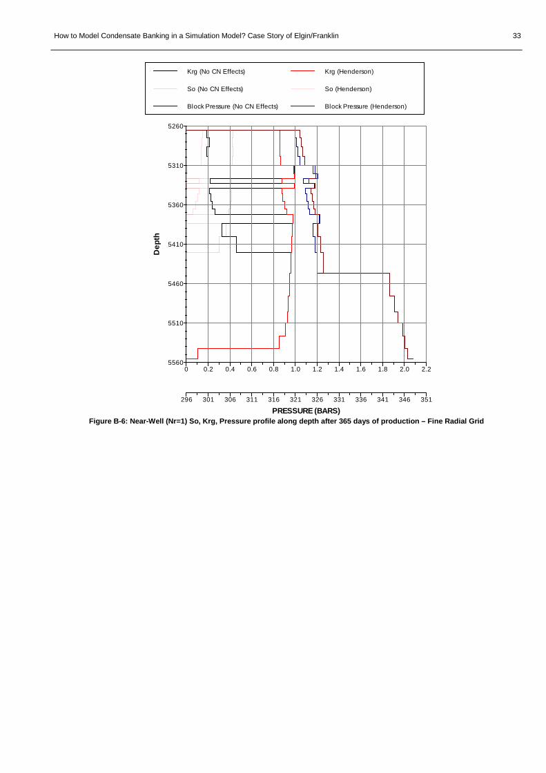
How to Model Condensate Banking in a Simulation Model? Case Story of Elgin/Franklin 33
Figure B-6: Near-Well (Nr=1) So, Krg, Pressure profile along depth after 365 days of production – Fine Radial Grid
0 0.2 0.4 0.6 0.8 1.0 1.2 1.4 1.6 1.8 2.0 2.2
5260
5310
5360
5410
5460
5510
5560
Dep
th
296 301 306 311 316 321 326 331 336 341 346 351
PRESSURE (BARS)
Krg (No CN Effects) Krg (Henderson)
So (No CN Effects) So (Henderson)
Block Pressure (No CN Effects) Block Pressure (Henderson)
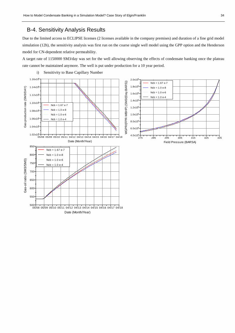
How to Model Condensate Banking in a Simulation Model? Case Story of Elgin/Franklin 34
B-4. Sensitivity Analysis Results Due to the limited access to ECLIPSE licenses (2 licenses available in the company premises) and duration of a fine grid model
simulation (12h), the sensitivity analysis was first run on the coarse single well model using the GPP option and the Henderson
model for CN-dependent relative permeability.
A target rate of 1150000 SM3/day was set for the well allowing observing the effects of condensate banking once the plateau
rate cannot be maintained anymore. The well is put under production for a 10 year period.
i) Sensitivity to Base Capillary Number
05/08 05/09 05/10 05/11 04/12 04/13 04/14 04/15 04/16 04/17 04/18
Date (Month/Year)
61.02x10
61.04x10
61.06x10
61.08x10
61.10x10
61.12x10
61.14x10
61.16x10
Gas
pro
duct
ion
rate
(SM
3/D
AY)
Ncb = 1.67 e-7
Ncb = 1.0 e-8
Ncb = 1.0 e-6
Ncb = 1.0 e-4
275 285 295 305 315 325 335
Field Pressure (BARSA)
44.0x10
46.0x10
48.0x10
51.0x10
51.2x10
51.4x10
51.6x10
51.8x10
52.0x10
WG
PR/(F
PR
-WB
HP
) (SM
3/(D
ay.B
ARS)
)
Ncb = 1.67 e-7
Ncb = 1.0 e-8
Ncb = 1.0 e-6
Ncb = 1.0 e-4
05/08 05/09 05/10 05/11 04/12 04/13 04/14 04/15 04/16 04/17 04/18
Date (Month/Year)
500
550
600
650
700
750
800
850
Gas
-oil
ratio
(SM
3/S
M3)
Ncb = 1.67 e-7
Ncb = 1.0 e-8
Ncb = 1.0 e-6
Ncb = 1.0 e-4

How to Model Condensate Banking in a Simulation Model? Case Story of Elgin/Franklin 35
ii) Sensitivity to coefficient mo
mo controls the critical oil saturation, however it does not have an impact on the relative permeability explaining why
productivity is not affected by mo but a change in producing GOR can be observed with increasing value of mo.
iii) Sensitivity to coefficient mg
mg does not affect productivity as the gas saturation around the well remains above the critical saturation.
05/08 05/09 05/10 05/11 04/12 04/13 04/14 04/15 04/16 04/17 04/18
Date (Month/Year)
61.02x10
61.04x10
61.06x10
61.08x10
61.10x10
61.12x10
61.14x10
61.16x10
Gas
pro
duct
ion
rate
(SM
3/D
AY)
mo = 0
mo = 10
mo = 20
mo = 40
275 285 295 305 315 325 335
Field Pressure (BARSA)
44.0x10
46.0x10
48.0x10
51.0x10
51.2x10
51.4x10
51.6x10
51.8x10
52.0x10
WG
PR/(F
PR
-WB
HP
) (SM
3/(D
ay.B
ARS)
)
mo = 0
mo = 10
mo = 20
mo = 40
05/08 05/09 05/10 05/11 04/12 04/13 04/14 04/15 04/16 04/17 04/18
Date (Month/Year)
500
550
600
650
700
750
800
850
Gas
-oil
ratio
(SM
3/S
M3)
mo = 0
mo = 10
mo = 20
mo = 40
05/08 05/09 05/10 05/11 04/12 04/13 04/14 04/15 04/16 04/17 04/18
Date (Month/Year)
61.02x10
61.04x10
61.06x10
61.08x10
61.10x10
61.12x10
61.14x10
61.16x10
Gas
pro
duct
ion
rate
(SM
3/D
AY)
mg = 0
mg = 10
mg = 20
mg = 40
275 285 295 305 315 325 335
Field Pressure (BARSA)
44.0x10
46.0x10
48.0x10
51.0x10
51.2x10
51.4x10
51.6x10
51.8x10
52.0x10
WG
PR/(F
PR
-WB
HP
) (SM
3/(D
ay.B
ARS)
)
mg = 0
mg = 10
mg = 20
mg = 40
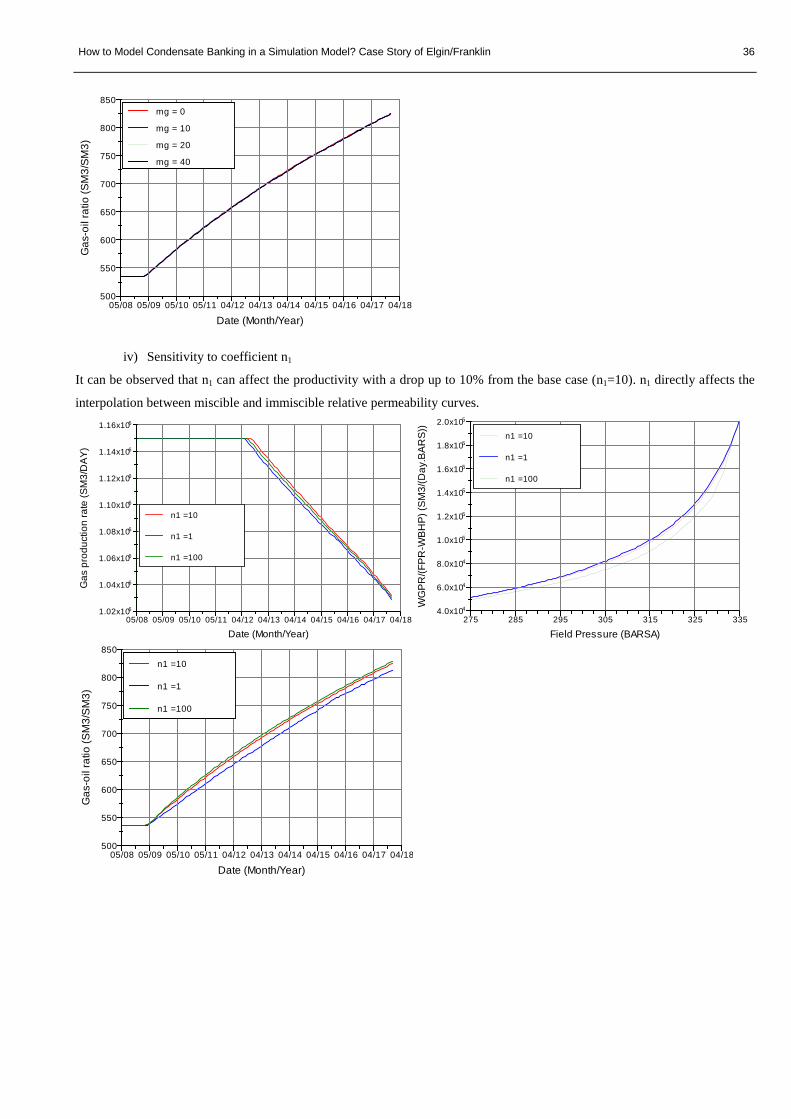
How to Model Condensate Banking in a Simulation Model? Case Story of Elgin/Franklin 36
iv) Sensitivity to coefficient n1
It can be observed that n1 can affect the productivity with a drop up to 10% from the base case (n1=10). n1 directly affects the
interpolation between miscible and immiscible relative permeability curves.
05/08 05/09 05/10 05/11 04/12 04/13 04/14 04/15 04/16 04/17 04/18
Date (Month/Year)
500
550
600
650
700
750
800
850
Gas
-oil
ratio
(SM
3/S
M3)
mg = 0
mg = 10
mg = 20
mg = 40
05/08 05/09 05/10 05/11 04/12 04/13 04/14 04/15 04/16 04/17 04/18
Date (Month/Year)
61.02x10
61.04x10
61.06x10
61.08x10
61.10x10
61.12x10
61.14x10
61.16x10
Gas
pro
duct
ion
rate
(SM
3/D
AY)
n1 =10
n1 =1
n1 =100
275 285 295 305 315 325 335
Field Pressure (BARSA)
44.0x10
46.0x10
48.0x10
51.0x10
51.2x10
51.4x10
51.6x10
51.8x10
52.0x10W
GPR
/(FP
R-W
BH
P) (
SM3/
(Day
.BAR
S))
n1 =10
n1 =1
n1 =100
05/08 05/09 05/10 05/11 04/12 04/13 04/14 04/15 04/16 04/17 04/18
Date (Month/Year)
500
550
600
650
700
750
800
850
Gas
-oil
ratio
(SM
3/S
M3)
n1 =10
n1 =1
n1 =100

How to Model Condensate Banking in a Simulation Model? Case Story of Elgin/Franklin 37
v) Sensitivity to coefficient n1o
The productivity loss reported in B-4.iv) is mainly attributable to n1o. This can be explained by the fact with higher value of mo
the oil CN-dependent relative permability is closer to the miscible relative permeability curve. The oil can flow more easily
and more gas needs to condensate to support the extra oil production.
05/08 05/09 05/10 05/11 04/12 04/13 04/14 04/15 04/16 04/17 04/18
Date (Month/Year)
61.02x10
61.04x10
61.06x10
61.08x10
61.10x10
61.12x10
61.14x10
61.16x10
Gas
pro
duct
ion
rate
(SM
3/D
AY)
n1o = n1g = 10n1o = n1g = 1n1o = n1g = 100n1o = 1; n1g = 10n1o = 100; n1g = 10
275 285 295 305 315 325 335
Field Pressure (BARSA)
44.0x10
46.0x10
48.0x10
51.0x10
51.2x10
51.4x10
51.6x10
51.8x10
52.0x10
WG
PR/(F
PR
-WB
HP
) (SM
3/(D
ay.B
ARS)
)
n1o = n1g = 10n1o = n1g = 1n1o = n1g = 100n1o = 1 ; n1g = 10n1o = 100 ; n1g = 10
05/08 05/09 05/10 05/11 04/12 04/13 04/14 04/15 04/16 04/17 04/18
Date (Month/Year)
500
550
600
650
700
750
800
850
Gas
-oil
ratio
(SM
3/S
M3)
n1o = n1g = 10n1o = n1g = 1n1o = n1g = 100n1o = 1; n1g = 10n1o = 100; n1g = 10
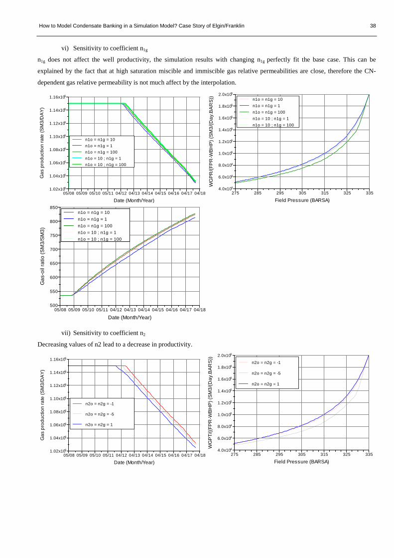
How to Model Condensate Banking in a Simulation Model? Case Story of Elgin/Franklin 38
vi) Sensitivity to coefficient n1g
n1g does not affect the well productivity, the simulation results with changing n1g perfectly fit the base case. This can be
explained by the fact that at high saturation miscible and immiscible gas relative permeabilities are close, therefore the CN-
dependent gas relative permeability is not much affect by the interpolation.
vii) Sensitivity to coefficient n2
Decreasing values of n2 lead to a decrease in productivity.
05/08 05/09 05/10 05/11 04/12 04/13 04/14 04/15 04/16 04/17 04/18
Date (Month/Year)
61.02x10
61.04x10
61.06x10
61.08x10
61.10x10
61.12x10
61.14x10
61.16x10
Gas
pro
duct
ion
rate
(SM
3/D
AY)
n1o = n1g = 10n1o = n1g = 1n1o = n1g = 100n1o = 10 ; n1g = 1 n1o = 10 ; n1g = 100
275 285 295 305 315 325 335
Field Pressure (BARSA)
44.0x10
46.0x10
48.0x10
51.0x10
51.2x10
51.4x10
51.6x10
51.8x10
52.0x10
WG
PR/(F
PR
-WB
HP
) (SM
3/(D
ay.B
ARS)
)
n1o = n1g = 10n1o = n1g = 1n1o = n1g = 100n1o = 10 ; n1g = 1 n1o = 10 ; n1g = 100
05/08 05/09 05/10 05/11 04/12 04/13 04/14 04/15 04/16 04/17 04/18
Date (Month/Year)
500
550
600
650
700
750
800
850
Gas
-oil
ratio
(SM
3/S
M3)
n1o = n1g = 10n1o = n1g = 1n1o = n1g = 100n1o = 10 ; n1g = 1 n1o = 10 ; n1g = 100
05/08 05/09 05/10 05/11 04/12 04/13 04/14 04/15 04/16 04/17 04/18
Date (Month/Year)
61.02x10
61.04x10
61.06x10
61.08x10
61.10x10
61.12x10
61.14x10
61.16x10
Gas
pro
duct
ion
rate
(SM
3/D
AY)
n2o = n2g = -1
n2o = n2g = -5
n2o = n2g = 1
275 285 295 305 315 325 335
Field Pressure (BARSA)
44.0x10
46.0x10
48.0x10
51.0x10
51.2x10
51.4x10
51.6x10
51.8x10
52.0x10
WG
PT/
((FP
R-W
BH
P) (
SM
3/(D
ay.B
AR
S))
n2o = n2g = -1
n2o = n2g = -5
n2o = n2g = 1

How to Model Condensate Banking in a Simulation Model? Case Story of Elgin/Franklin 39
viii) Sensitivity analysis run on fine grid
Figure B-7: Base Capillary Number effect on productivity
Figure B-8: Effect of modelling only krg or krg and kro
Figure B-9: Sensitivity of well productivity as a function of n1
05/08 05/09 05/10 05/11 04/12 04/13 04/14 04/15 04/16 04/17 04/18
Date (Month/Year)
500
550
600
650
700
750
800
850G
as-o
il ra
tio (S
M3/
SM
3)
n2o = n2g = -1
n2o = n2g = -5
n2o = n2g = 1
308 312 316 320 324 328 332 336 340
Field Pressure (BARSa)
0
45.0x10
51.0x10
51.5x10
52.0x10
52.5x10
53.0x10
WG
PR/(F
PR-W
BHP)
(SM
3/(D
ay.B
ARSa
))
Ncb = 1.67e-7
Ncb = 1e-5
Ncb = 1e-8
308 312 316 320 324 328 332 336 340
(BARSA)
0
45.0x10
51.0x10
51.5x10
52.0x10
52.5x10
53.0x10
WG
PR/(F
PR-W
BHP)
(SM
3/(D
ay.B
ARSa
))
Henderson - both krg and kro modeled
Henderson - only krg modeled
Whitson - only krg modeled
308 312 316 320 324 328 332 336 340
Field Pressure (BARSa)
0
45.0x10
51.0x10
51.5x10
52.0x10
52.5x10
53.0x10
WG
PR/(F
PR-W
BHP)
(SM
3/(D
AY.B
ARSa
))
n1=1n1=5n1=10n1=15n1=20
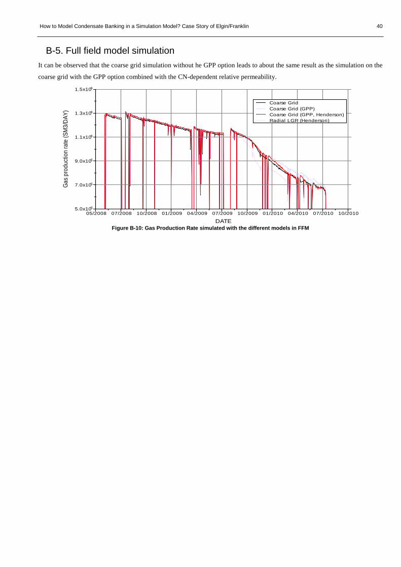
How to Model Condensate Banking in a Simulation Model? Case Story of Elgin/Franklin 40
B-5. Full field model simulation It can be observed that the coarse grid simulation without he GPP option leads to about the same result as the simulation on the
coarse grid with the GPP option combined with the CN-dependent relative permeability.
Figure B-10: Gas Production Rate simulated with the different models in FFM
05/2008 07/2008 10/2008 01/2009 04/2009 07/2009 10/2009 01/2010 04/2010 07/2010 10/2010
DATE
55.0x10
57.0x10
59.0x10
61.1x10
61.3x10
61.5x10
Gas p
rodu
ction
rate
(SM
3/DA
Y)
Coarse GridCoarse Grid (GPP)Coarse Grid (GPP, Henderson)Radial LGR (Henderson)
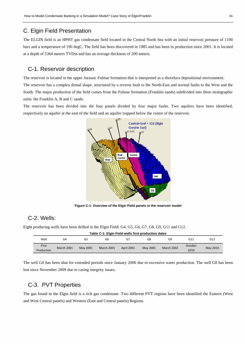
How to Model Condensate Banking in a Simulation Model? Case Story of Elgin/Franklin 41
C. Elgin Field Presentation The ELGIN field is an HPHT gas condensate field located in the Central North Sea with an initial reservoir pressure of 1100
bars and a temperature of 190 degC. The field has been discovered in 1985 and has been in production since 2001. It is located
at a depth of 5364 meters TVDss and has an average thickness of 200 meters.
C-1. Reservoir description The reservoir is located in the upper Jurassic Fulmar formation that is interpreted as a shoreface depositional environment.
The reservoir has a complex domal shape, structured by a reverse fault to the North-East and normal faults to the West and the
South. The major production of the field comes from the Fulmar formation (Franklin sands) subdivided into three stratigraphic
units: the Franklin A, B and C sands.
The reservoir has been divided into the four panels divided by four major faults. Two aquifers have been identified,
respectively an aquifer at the east of the field and an aquifer trapped below the centre of the reservoir.
Figure C-1: Overview of the Elgin Field panels in the reservoir model
C-2. Wells: Eight producing wells have been drilled in the Elgin Field: G4, G5, G6, G7, G8, G9, G11 and G12.
Table C-1: Elgin Field wells first production dates Well G4 G5 G6 G7 G8 G9 G11 G12
First Production
March 2001 May 2001 March 2001 April 2001 May 2001 March 2002 October
2010 May 2010
The well G6 has been shut for extended periods since January 2006 due to excessive water production. The well G8 has been
lost since November 2009 due to casing integrity issues.
C-3. PVT Properties The gas found in the Elgin field is a rich gas condensate. Two different PVT regions have been identified the Eastern (West
and West Central panels) and Western (East and Central panels) Regions.

How to Model Condensate Banking in a Simulation Model? Case Story of Elgin/Franklin 42
Table C-2: Elgin West Gas composition Component East West
Mol % Mol % N2 0.64 0.51
CO2 2.37 3 C1 62.94 68.15 C2 8.91 8.2 C3 4.79 3.94 iC4 1.02 0.81 nC4 2.17 1.7 iC5 1.07 0.96 nC5 1.13 0.89 C6 2.36 1.86 C7 2.47 2.01 C8 2.04 1.6 C9 1.43 1.15
C10 1.29 0.98 CN1 3.07 2.55 CN2 2.07 1.46 CN3 0.23 0.23
Figure C-2: Elgin-West PVT Phase envelope
Figure C-3: Elgin-West Liquid condensation curve
C-4. Production Profiles The following production data were used as matching criteria in the objective function definition.
0
5
10
15
20
25
0 100 200 300 400
Liqu
id C
onde
nsat
ion
(% v
olum
e)
Pressure, BARa

How to Model Condensate Banking in a Simulation Model? Case Story of Elgin/Franklin 43
Figure C-4: Elgin Field Gas Production Rates
Figure C-5: Elgin Field Water Production Rates

How to Model Condensate Banking in a Simulation Model? Case Story of Elgin/Franklin 44
Figure C-6: Elgin Field Historical Production Rate
The THP for each well was used as controlling parameter for the well production in the dynamic simulation model.
Figure C-7: Well G4 Tubing Head Pressure (THP, BARA) historical data
Figure C-8: Well G4 GOR historical data
Due to the lack of individual well data for the Elgin field, it is difficult to identify the effect of condensate banking on the
production. The producing GOR however significantly increases once the pressure in the reservoir falls below the dew point.
How to Model Condensate Banking in a Simulation Model? Case Story of Elgin/Franklin 45
From Figure C-8 we can see that the pressure around the well G4 has fallen below the dew point around 3000 days after first
production (in November 2009). Besides the uncertainty added from the back allocation process (10%) make it difficult to
identify rate changes directly as only the THP measurement is available.
C-5. Simulation model A complete compositional simulation package running on Eclipse 300 has been made available for the purpose of purpose of
the project. The model base is the 2P case identified by the Operator. The geometry of the reservoir is described using corner
point gridding and the faults are identified. The model contains the existing separator properties, the PVT and equilibrium
properties for the fluids in place in the different compartments identified in the reservoir. The model has been used and refined
since 2005 for history matching and production prediction purpose. Therefore it includes multipliers for faults and layer
transmissibility. The relative permeability model used in the simulation is complex as it includes 53 relative permeability
tables. The choke, the tubing head pressure, the back-allocated production rates and cumulative production (Gas, Oil, Water)
are available for each well. Given that the production for each well is back allocated based on THP measurement, backpressure
and well test data, the history matching has and will be performed using THP (Tubing Head Pressure) controls. The well
production in the simulation model is control by THP input. In the current manually HM model the THP are defined on a daily
basis, with this input the simulation runs in 3.5 hours.
Previous studies have been performed to identify the sensitivity of the model to the aquifer pore volume, the faults
transmissibility, the mobility around the wells and the skin. It has been identified from the previous studies that the panels
containing the wells G4 and G5 are in communication through the observation of the same pressure trends in both panels. The
panels containing the wells G6 and G7 are isolated as the pressure evolved differently in both panels. PVT analysis reports
corroborated these interpretations as different fluid properties were observed between the G6 panel and the other panels.
The simulation model uses a 7 component model with Peng-Robinson equation of state.
The reservoir temperature has been defined for the different regions of the reservoir: Table C-3: Elgin Field regions temperature PVT Region Temperature (DegC)
1 188.4 2 188.7 3 188.4 4 192.5
C-6. Petrophysical properties The reports made available provide a general description of the properties of each layer/facies association:
- Average porosity and lower and upper limits
- Porosity decreasing trend with depth by facies
- K/Phi relationship ( logK = A * Phi + B )
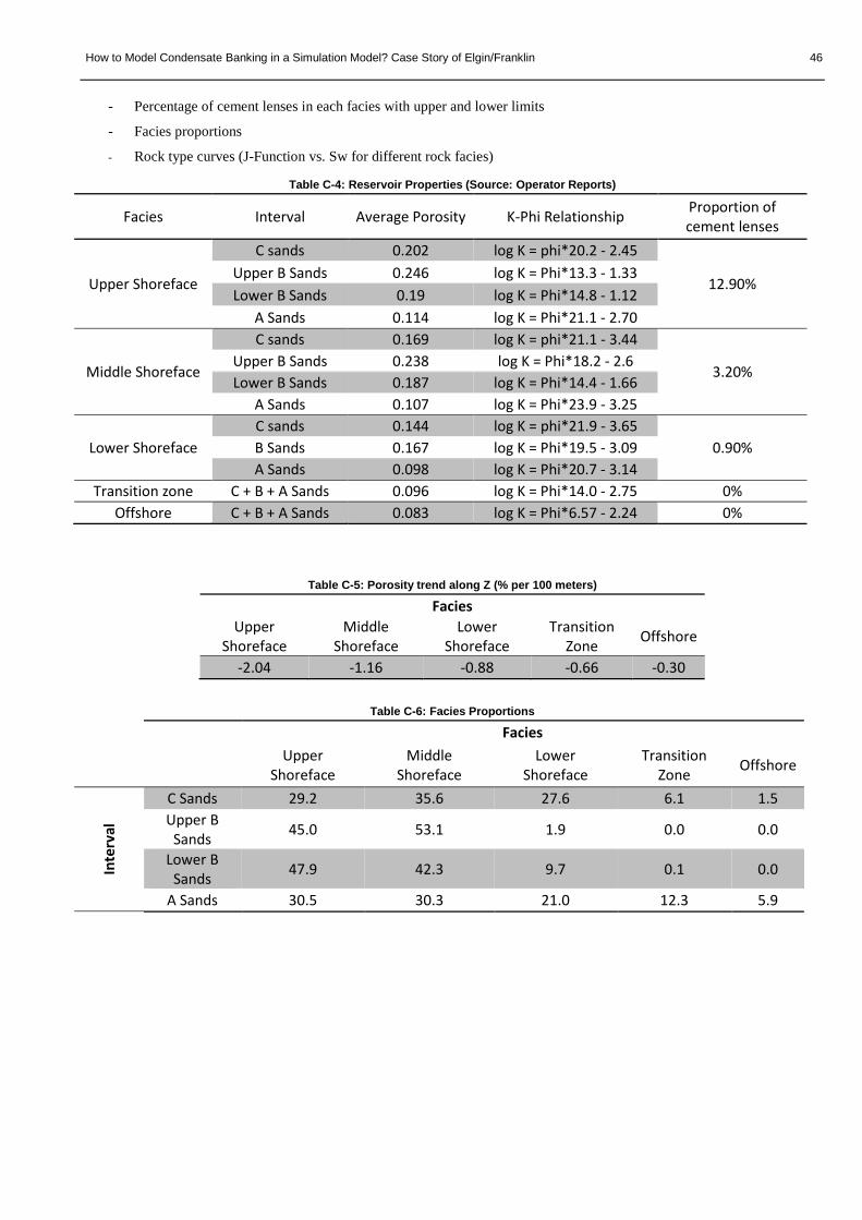
How to Model Condensate Banking in a Simulation Model? Case Story of Elgin/Franklin 46
- Percentage of cement lenses in each facies with upper and lower limits
- Facies proportions
- Rock type curves (J-Function vs. Sw for different rock facies)
Table C-4: Reservoir Properties (Source: Operator Reports)
Facies Interval Average Porosity K-Phi Relationship Proportion of cement lenses
Upper Shoreface
C sands 0.202 log K = phi*20.2 - 2.45
12.90% Upper B Sands 0.246 log K = Phi*13.3 - 1.33 Lower B Sands 0.19 log K = Phi*14.8 - 1.12
A Sands 0.114 log K = Phi*21.1 - 2.70
Middle Shoreface
C sands 0.169 log K = phi*21.1 - 3.44
3.20% Upper B Sands 0.238 log K = Phi*18.2 - 2.6 Lower B Sands 0.187 log K = Phi*14.4 - 1.66
A Sands 0.107 log K = Phi*23.9 - 3.25
Lower Shoreface C sands 0.144 log K = phi*21.9 - 3.65
0.90% B Sands 0.167 log K = Phi*19.5 - 3.09 A Sands 0.098 log K = Phi*20.7 - 3.14
Transition zone C + B + A Sands 0.096 log K = Phi*14.0 - 2.75 0% Offshore C + B + A Sands 0.083 log K = Phi*6.57 - 2.24 0%
Table C-5: Porosity trend along Z (% per 100 meters)
Facies Upper
Shoreface Middle
Shoreface Lower
Shoreface Transition
Zone Offshore
-2.04 -1.16 -0.88 -0.66 -0.30
Table C-6: Facies Proportions
Facies Upper
Shoreface Middle
Shoreface Lower
Shoreface Transition
Zone Offshore
Inte
rval
C Sands 29.2 35.6 27.6 6.1 1.5 Upper B
Sands 45.0 53.1 1.9 0.0 0.0
Lower B Sands 47.9 42.3 9.7 0.1 0.0
A Sands 30.5 30.3 21.0 12.3 5.9
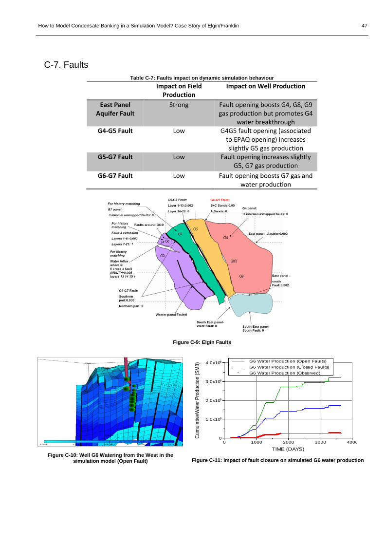
How to Model Condensate Banking in a Simulation Model? Case Story of Elgin/Franklin 47
C-7. Faults Table C-7: Faults impact on dynamic simulation behaviour
Impact on Field Production
Impact on Well Production
East Panel Aquifer Fault
Strong Fault opening boosts G4, G8, G9 gas production but promotes G4
water breakthrough G4-G5 Fault Low G4G5 fault opening (associated
to EPAQ opening) increases slightly G5 gas production
G5-G7 Fault Low Fault opening increases slightly G5, G7 gas production
G6-G7 Fault Low Fault opening boosts G7 gas and water production
Figure C-9: Elgin Faults
Figure C-10: Well G6 Watering from the West in the
simulation model (Open Fault)
Figure C-11: Impact of fault closure on simulated G6 water production
0 1000 2000 3000 4000
TIME (DAYS)
0
61.0x10
62.0x10
63.0x10
64.0x10
Cum
ulat
iveW
ater
Pro
ducti
on (S
M3)
G6 Water Production (Open Faults)G6 Water Production (Closed Faults)G6 Water Production (Observed)
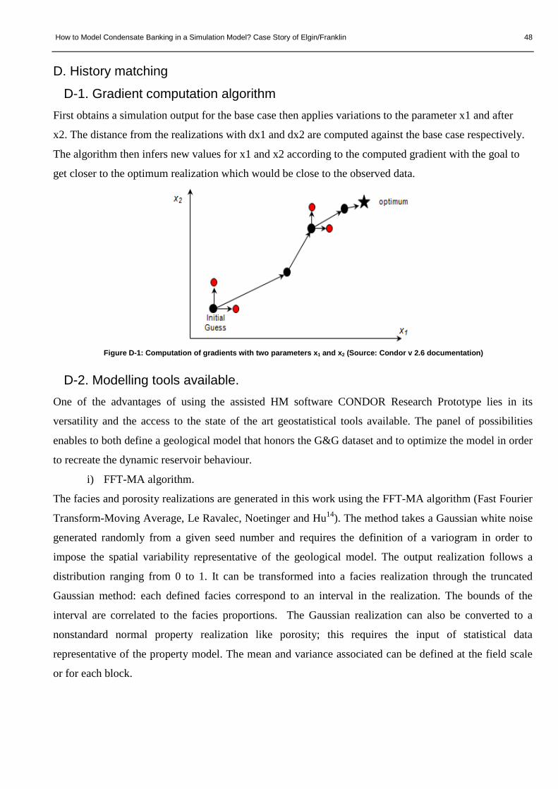
How to Model Condensate Banking in a Simulation Model? Case Story of Elgin/Franklin 48
D. History matching
D-1. Gradient computation algorithm First obtains a simulation output for the base case then applies variations to the parameter x1 and after
x2. The distance from the realizations with dx1 and dx2 are computed against the base case respectively.
The algorithm then infers new values for x1 and x2 according to the computed gradient with the goal to
get closer to the optimum realization which would be close to the observed data.
Figure D-1: Computation of gradients with two parameters x1 and x2 (Source: Condor v 2.6 documentation)
D-2. Modelling tools available.
One of the advantages of using the assisted HM software CONDOR Research Prototype lies in its
versatility and the access to the state of the art geostatistical tools available. The panel of possibilities
enables to both define a geological model that honors the G&G dataset and to optimize the model in order
to recreate the dynamic reservoir behaviour.
i) FFT-MA algorithm.
The facies and porosity realizations are generated in this work using the FFT-MA algorithm (Fast Fourier
Transform-Moving Average, Le Ravalec, Noetinger and Hu14). The method takes a Gaussian white noise
generated randomly from a given seed number and requires the definition of a variogram in order to
impose the spatial variability representative of the geological model. The output realization follows a
distribution ranging from 0 to 1. It can be transformed into a facies realization through the truncated
Gaussian method: each defined facies correspond to an interval in the realization. The bounds of the
interval are correlated to the facies proportions. The Gaussian realization can also be converted to a
nonstandard normal property realization like porosity; this requires the input of statistical data
representative of the property model. The mean and variance associated can be defined at the field scale
or for each block.
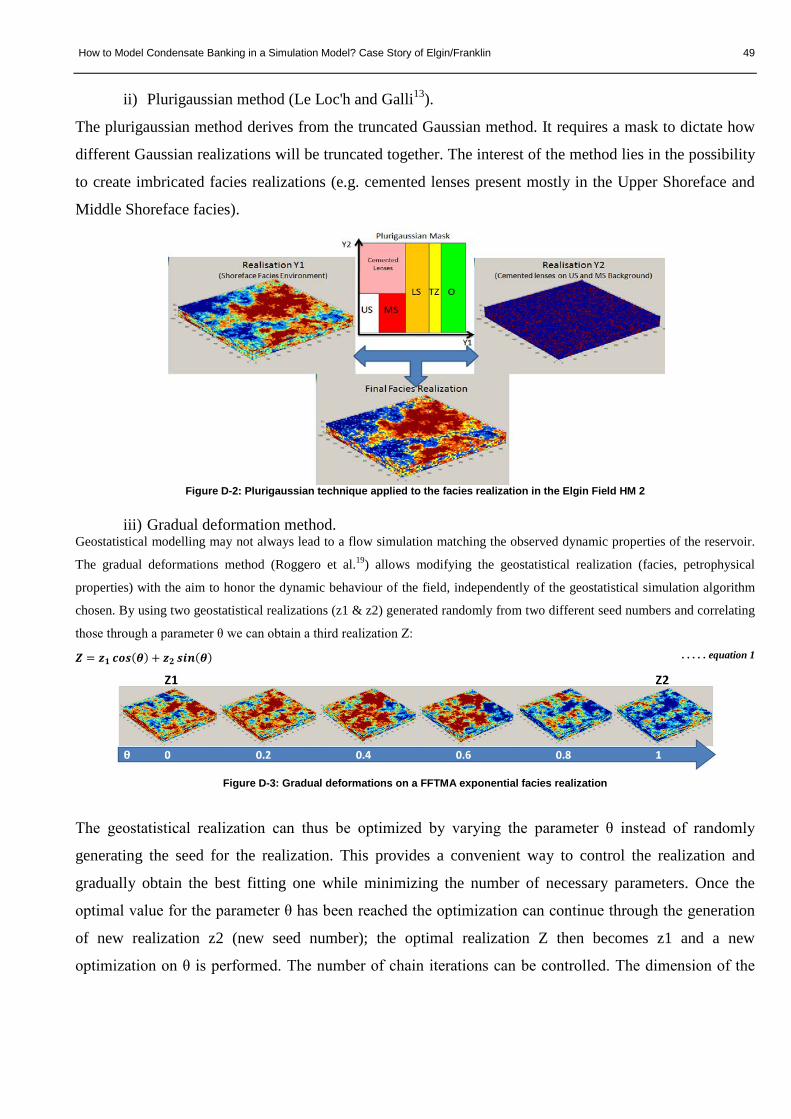
How to Model Condensate Banking in a Simulation Model? Case Story of Elgin/Franklin 49
ii) Plurigaussian method (Le Loc'h and Galli13).
The plurigaussian method derives from the truncated Gaussian method. It requires a mask to dictate how
different Gaussian realizations will be truncated together. The interest of the method lies in the possibility
to create imbricated facies realizations (e.g. cemented lenses present mostly in the Upper Shoreface and
Middle Shoreface facies).
Figure D-2: Plurigaussian technique applied to the facies realization in the Elgin Field HM 2
iii) Gradual deformation method.
Geostatistical modelling may not always lead to a flow simulation matching the observed dynamic properties of the reservoir.
The gradual deformations method (Roggero et al.19) allows modifying the geostatistical realization (facies, petrophysical
properties) with the aim to honor the dynamic behaviour of the field, independently of the geostatistical simulation algorithm
chosen. By using two geostatistical realizations (z1 & z2) generated randomly from two different seed numbers and correlating
those through a parameter θ we can obtain a third realization Z:
𝒁𝒁 = 𝒛𝒛𝟏𝟏 𝒄𝒄𝒐𝒐𝒄𝒄(𝜽𝜽) + 𝒛𝒛𝟐𝟐 𝒄𝒄𝒔𝒔𝒏𝒏(𝜽𝜽) . . . . . equation 1
Figure D-3: Gradual deformations on a FFTMA exponential facies realization
The geostatistical realization can thus be optimized by varying the parameter θ instead of randomly
generating the seed for the realization. This provides a convenient way to control the realization and
gradually obtain the best fitting one while minimizing the number of necessary parameters. Once the
optimal value for the parameter θ has been reached the optimization can continue through the generation
of new realization z2 (new seed number); the optimal realization Z then becomes z1 and a new
optimization on θ is performed. The number of chain iterations can be controlled. The dimension of the
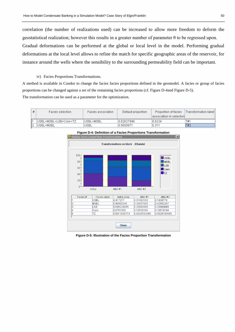
How to Model Condensate Banking in a Simulation Model? Case Story of Elgin/Franklin 50
correlation (the number of realizations used) can be increased to allow more freedom to deform the
geostatistical realization; however this results in a greater number of parameter θ to be regressed upon.
Gradual deformations can be performed at the global or local level in the model. Performing gradual
deformations at the local level allows to refine the match for specific geographic areas of the reservoir, for
instance around the wells where the sensibility to the surrounding permeability field can be important.
iv) Facies Proportions Transformations.
A method is available in Condor to change the facies facies proportions defined in the geomodel. A facies or group of facies
proportions can be changed against a set of the remaining facies proportions (cf. Figure D-4and Figure D-5).
The transformation can be used as a parameter for the optimization.
Figure D-4: Definition of a Facies Proportions Transformation
Figure D-5: Illustration of the Facies Proportion Transformation
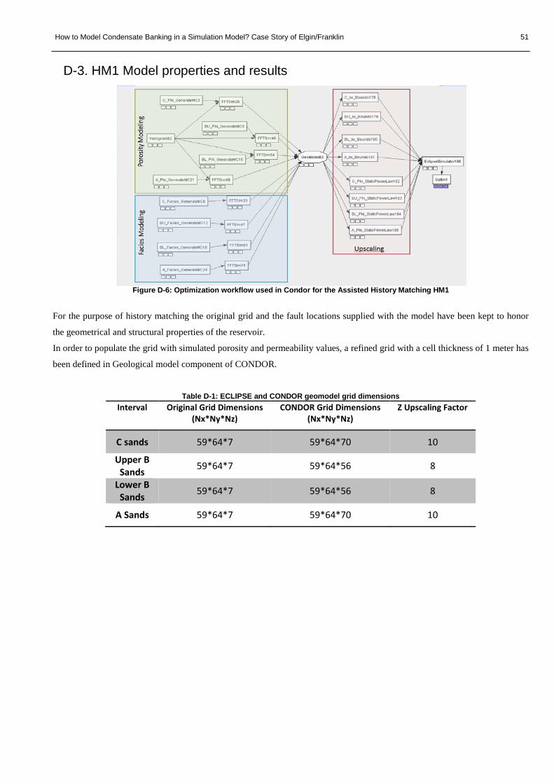
How to Model Condensate Banking in a Simulation Model? Case Story of Elgin/Franklin 51
D-3. HM1 Model properties and results
Figure D-6: Optimization workflow used in Condor for the Assisted History Matching HM1
For the purpose of history matching the original grid and the fault locations supplied with the model have been kept to honor
the geometrical and structural properties of the reservoir.
In order to populate the grid with simulated porosity and permeability values, a refined grid with a cell thickness of 1 meter has
been defined in Geological model component of CONDOR.
Table D-1: ECLIPSE and CONDOR geomodel grid dimensions Interval Original Grid Dimensions
(Nx*Ny*Nz) CONDOR Grid Dimensions
(Nx*Ny*Nz) Z Upscaling Factor
C sands 59*64*7 59*64*70 10
Upper B Sands 59*64*7 59*64*56 8
Lower B Sands 59*64*7 59*64*56 8
A Sands 59*64*7 59*64*70 10

How to Model Condensate Banking in a Simulation Model? Case Story of Elgin/Franklin 52
Figure D-7: Reservoir structure description in Condor R&D
The dimensions of the grid were chosen to account as closely as possible for the structure of the existing 2P reservoir model.
The geomodel described in CONDOR was simplified to include only two facies: a sandstone background and cemented beds.
The sandstone background facies is representative of the five facies described in the shoreface depositional environment, its
average properties vary linearly along the Y axis and Z axis to account for the progressive change the transition from upper
shoreface to offshore facies implies.
i) Facies properties
Cement lenses: The sandstone facies is the background facies for the geomodel, the average cemented beds facies proportions
varies linearly from 12.9% for Y=1to 0% for Y=64. No variation is performed along the Z axis. The cement lenses have been
interpreted to extend over 100 m x 100 m and to have no porosity and permeability.
Sandstone background: The average porosity distribution for the sandstone facies in each interval was calculated using a trend
along the Y axis resulting from a linear interpolation between the average porosity value observed in the upper shoreface
depositional environment and the average value observed in the offshore depositional environment (cf. Table C-4).This
solution was chosen due to the lack of information in the reports available on facies proportions and distributions at first. The
porosity was also given a decreasing trend along the Z axis as described in the Operator report.
The horizontal permeability for the sandstone background is calculated using a log K = f(phi) function. It has been derived
through a linear interpolation of the permeability calculated for each interval/facies association using the K-Phi correlation
available in the Operator’s report.

How to Model Condensate Banking in a Simulation Model? Case Story of Elgin/Franklin 53
Figure D-8: Determination of base value for log(K) = f(phi) function
The vertical permeability is calculated through multiplication of the horizontal permeability by a coefficient.
ii) Upscaling
The upscaling for the horizontal permeability is performed using Cardwell & Parsons method. The porosity is upscaled using
arithmetic average weighed for bulk volume.
Figure D-9: Upscaled Porosity realization for simplified two facies model
iii) Optimization HM 1
For HM1 only the FGPT data (Field Cumulative Gas Production) was used in the objective function definition. The weight was
left as default with a constant confidence interval of 1.23x10⁹ sm3.
If we compare other production data, e.g. field cumulative water production and well production rates we can see that the
matched model behaviour still remains far from the actual field production. Therefore more parameters should be introduced to
improve the quality of the match. This first attempt was performed on a full field deformation of the porosity and facies
realizations without trying to improve the quality of the match at the well scale. The first attempt used the 53 relative
permeability tables defined by the operator and the SATNUM grid definition of the Operator 2P reservoir model.
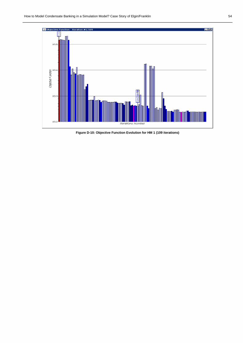
How to Model Condensate Banking in a Simulation Model? Case Story of Elgin/Franklin 54
Figure D-10: Objective Function Evolution for HM 1 (109 iterations)

How to Model Condensate Banking in a Simulation Model? Case Story of Elgin/Franklin 55
Table D-2: Match quality evolution for FGPT and FWPT between first and optimum iterations (HM1). Data First Iteration Optimum Iteration
FGPT
FWPT
D-4. Optimization HM2 The same geological model definition used in HM1 was used in HM2. This time the 53 sets relative permeability tables defined
by the operator were replaced by a single set of relative permeability defined using the LET correlation.
The parameters used for the second optimization were varied on a global field scale.
The optimization parameters defined are:
- Coefficients Ewo, Tw
o, Low and To
g for the LET correlations
- Swi
- A and B coefficents for the log(K)=f(Phi) relationship
- The vertical to horizontal Permeability Ratio
- Gradual deformations parameters for the porosity realizations in each interval
- Facies proportions transformations for the C and B intervals (proportion of cemented lenses)
New production data has been introduced for the objective function calculation: GOR for each well (WGOR), Total gas
production for each well (WGPT), Field total water production (FWPT)
The introduction of new production data required the adjustment of the relative contributions of the different well production
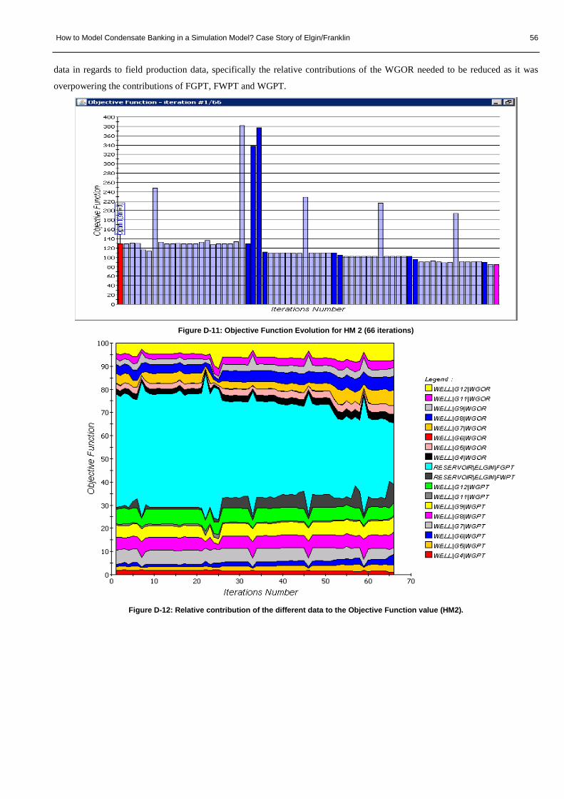
How to Model Condensate Banking in a Simulation Model? Case Story of Elgin/Franklin 56
data in regards to field production data, specifically the relative contributions of the WGOR needed to be reduced as it was
overpowering the contributions of FGPT, FWPT and WGPT.
Figure D-11: Objective Function Evolution for HM 2 (66 iterations)
Figure D-12: Relative contribution of the different data to the Objective Function value (HM2).

How to Model Condensate Banking in a Simulation Model? Case Story of Elgin/Franklin 57
Figure D-13: Contribution of the different data to the Objective Function value (HM2).
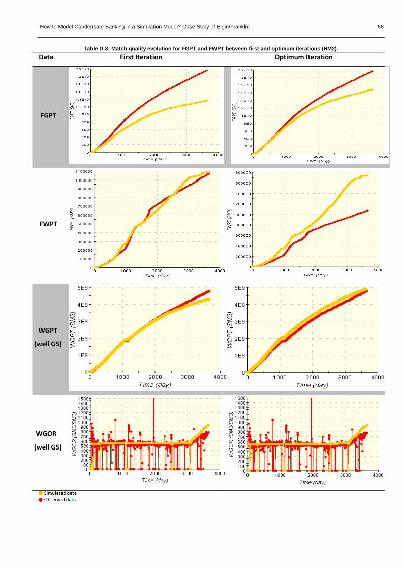
How to Model Condensate Banking in a Simulation Model? Case Story of Elgin/Franklin 58
Table D-3: Match quality evolution for FGPT and FWPT between first and optimum iterations (HM2). Data First Iteration Optimum Iteration
FGPT
FWPT
WGPT
(well G5)
WGOR
(well G5)

How to Model Condensate Banking in a Simulation Model? Case Story of Elgin/Franklin 59
D-5. Optimization HM3 For HM3 the geomodel definition was modified as new data became available: the facies proportions
described by the geologist for the Operator Geomodel. This time the optimization is made on the facies
realization and not the porosity realizations. The facies proportions transformations are included in the
optimization to control the average porosity or permeability of an interval. The plurigaussian method was
used to generate the facies realizations.
Figure D-14: Upscaled porosity realization for HM 3
The optimization parameters defined are:
- Coefficients Ewo, Tw
o, Low and To
g for the LET correlations
- Swi
- Fault transmissivity
- Gradual deformations parameters for the facies realizations in each interval
- Facies proportions transformations for the lower B interval and upper B interval
Figure D-15: Objective function evolution for the optimization HM3 (123 iterations)
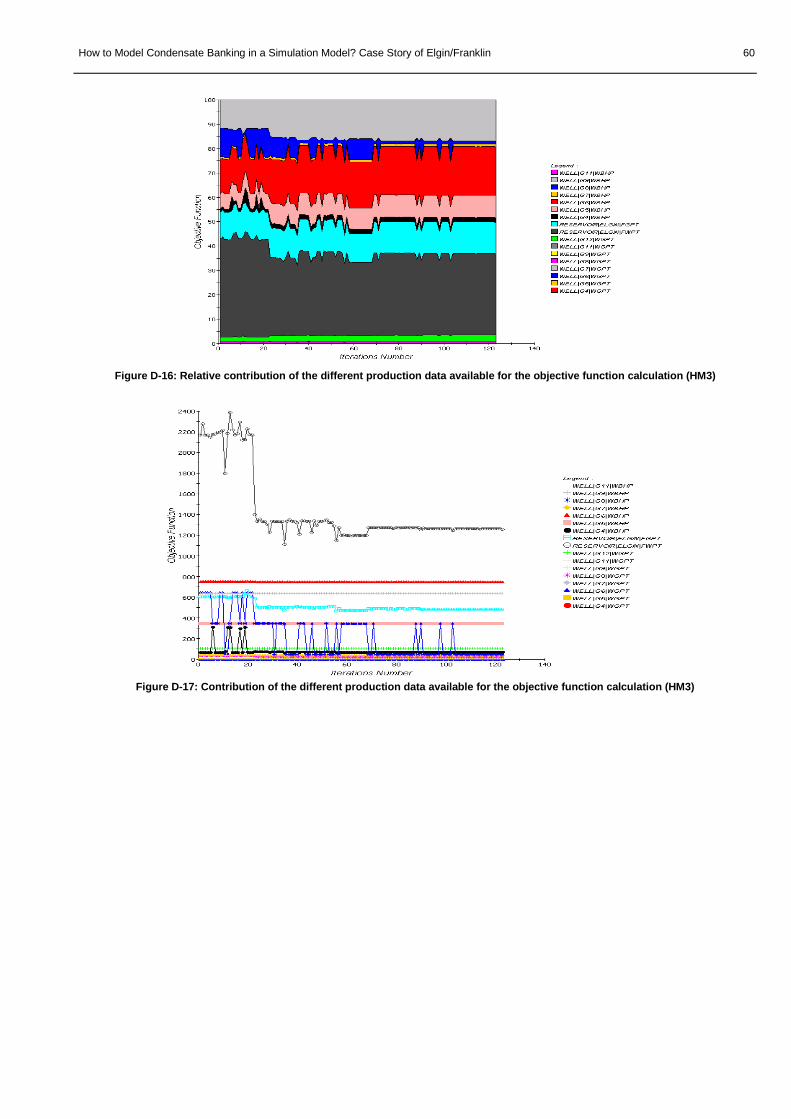
How to Model Condensate Banking in a Simulation Model? Case Story of Elgin/Franklin 60
Figure D-16: Relative contribution of the different production data available for the objective function calculation (HM3)
Figure D-17: Contribution of the different production data available for the objective function calculation (HM3)

How to Model Condensate Banking in a Simulation Model? Case Story of Elgin/Franklin 61
Table D-4: Match quality evolution for FGPT and FWPT between first and optimum iterations (HM3). Data First Iteration Optimum Iteration
FGPT
FWPT
The instability due to the WBHP objective function contribution is highlighted for the well G8.
Figure D-18: Contribution of the G8 BHP measurement to the objective function (HM3).

How to Model Condensate Banking in a Simulation Model? Case Story of Elgin/Franklin 62
Table D-5: Match quality evolution for the well G8 BHP and WGPT between first and optimum iterations (HM3). Data First Iteration Optimum Iteration
WBHP
(G8)
WGPT
(G8)
Figure D-19: G8 BHP simulated vs. observed for iteration #65 (HM3).

How to Model Condensate Banking in a Simulation Model? Case Story of Elgin/Franklin 63
D-6. Optimization HM4 Different relative permeability tables are introduced for each facies. The same set of coefficient is defined for the LET
correlation for each facies and the irreducible water saturation (Swi) is defined for the Upper shoreface facies. The other tables
are built through shifting the irreducible water saturation based on the rock type observations:
- Upper Shoreface: Swi
- Middle shoreface: Swi + 0.07
- Lower shoreface: Swi + 0.15
- Transition zone: Swi + 0.25
- Offshore: Swi + 0.35
Local gradual deformations zones were introduced in the Lower B interval to test the potential
improvement.
Figure D-20: Region for Local Grid Deformations
The optimization parameters defined are:
- Coefficients Ewo, Tw
o, Low and To
g for the LET correlations
- Swi
- Fault transmissivity
- Gradual deformations parameters for the facies realizations in each interval (zoned in Lower B interval)
- Facies proportions transformations for the lower B interval and upper B interval
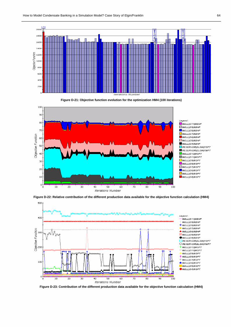
How to Model Condensate Banking in a Simulation Model? Case Story of Elgin/Franklin 64
Figure D-21: Objective function evolution for the optimization HM4 (100 iterations)
Figure D-22: Relative contribution of the different production data available for the objective function calculation (HM4)
Figure D-23: Contribution of the different production data available for the objective function calculation (HM4)

How to Model Condensate Banking in a Simulation Model? Case Story of Elgin/Franklin 65
Table D-6: Match quality evolution for FGPT and FWPT between first and optimum iterations (HM4). Data First Iteration Optimum Iteration
FGPT
FWPT
D-7. Optimization HM5 The BHP data was removed from the objective function computation. Only the field cumulative gas and water produced
volumes and each well cumulative gas volumes are used for the optimization.
The optimization parameters defined are:
- Coefficients Ewo, Tw
o, Low and To
g for the LET correlations
- Swi
- Fault transmissivity
- Gradual deformations parameters for the facies realizations in each interval (zoned in Lower B interval)
- Facies proportions transformations for the lower B interval
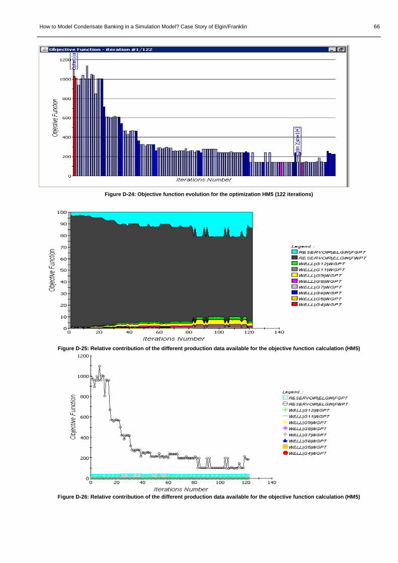
How to Model Condensate Banking in a Simulation Model? Case Story of Elgin/Franklin 66
Figure D-24: Objective function evolution for the optimization HM5 (122 iterations)
Figure D-25: Relative contribution of the different production data available for the objective function calculation (HM5)
Figure D-26: Relative contribution of the different production data available for the objective function calculation (HM5)
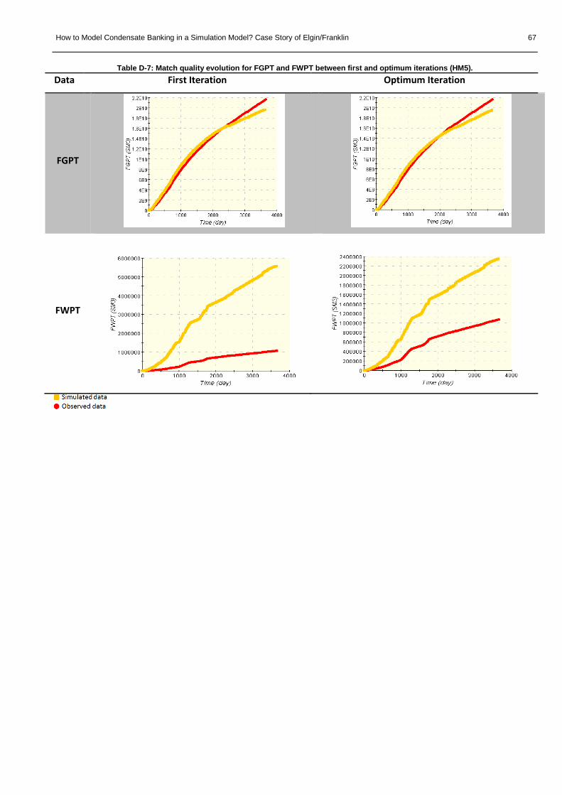
How to Model Condensate Banking in a Simulation Model? Case Story of Elgin/Franklin 67
Table D-7: Match quality evolution for FGPT and FWPT between first and optimum iterations (HM5). Data First Iteration Optimum Iteration
FGPT
FWPT

How to Model Condensate Banking in a Simulation Model? Case Story of Elgin/Franklin 68
E. LET Correlation
E-1. Description of the LET correlation The original reservoir model uses 53 relative permeability tables, to simplify the model the LET relative permeability
correlation (Lomeland, Ebeltoft and Thomas 2005) has been implemented in the HM and the coefficient were used as a
parameter for HM.
The correlation is defined with three parameters L, E and T to allow a better control on the shape of the relative permeability
curve over a broad range of saturation which is not possible with the Corey correlation.
The water saturation dependent water-oil relative permeability curves have been defined as follows:
𝑆𝑆𝑤𝑤𝑛𝑛 =𝑆𝑆𝑤𝑤 − 𝑆𝑆𝑤𝑤𝑤𝑤
1 − 𝑆𝑆𝑟𝑟𝑟𝑟𝑤𝑤 − 𝑆𝑆𝑤𝑤𝑤𝑤 . . . . . equation E-1
𝑘𝑘𝑟𝑟𝑤𝑤 = 𝑘𝑘𝑟𝑟𝑤𝑤𝑟𝑟𝑆𝑆𝑤𝑤𝑛𝑛𝐿𝐿𝑤𝑤
𝑜𝑜
𝑆𝑆𝑤𝑤𝑛𝑛𝐿𝐿𝑤𝑤𝑜𝑜
+ 𝐸𝐸𝑤𝑤𝑟𝑟 (1 − 𝑆𝑆𝑤𝑤𝑛𝑛)𝑇𝑇𝑤𝑤𝑜𝑜 . . . . . equation E-2
𝑘𝑘𝑟𝑟𝑟𝑟𝑤𝑤 = 𝑘𝑘𝑟𝑟𝑟𝑟𝑥𝑥(1 − 𝑆𝑆𝑤𝑤𝑛𝑛)𝐿𝐿𝑜𝑜𝑤𝑤
(1 − 𝑆𝑆𝑤𝑤𝑛𝑛)𝐿𝐿𝑜𝑜𝑤𝑤 + 𝐸𝐸𝑟𝑟𝑤𝑤𝑆𝑆𝑤𝑤𝑛𝑛𝑇𝑇𝑜𝑜𝑤𝑤
. . . . . equation E-3
𝑘𝑘𝑟𝑟𝑤𝑤𝑟𝑟 =(1 − 𝑆𝑆𝑤𝑤𝑤𝑤 − 𝑆𝑆𝑟𝑟𝑟𝑟𝑤𝑤)𝐿𝐿𝑤𝑤𝑘𝑘
(1 − 𝑆𝑆𝑤𝑤𝑤𝑤 − 𝑆𝑆𝑟𝑟𝑟𝑟𝑤𝑤)𝐿𝐿𝑤𝑤𝑘𝑘 + 𝐸𝐸𝑤𝑤𝑘𝑘𝑆𝑆𝑟𝑟𝑟𝑟𝑇𝑇𝑤𝑤𝑘𝑘
. . . . . equation E-4
𝑘𝑘𝑟𝑟𝑟𝑟𝑥𝑥 =(1 − 𝑆𝑆𝑤𝑤𝑤𝑤)𝐿𝐿𝑜𝑜
𝑘𝑘
(1 − 𝑆𝑆𝑤𝑤𝑤𝑤)𝐿𝐿𝑜𝑜𝑘𝑘 + 𝐸𝐸𝑟𝑟𝑘𝑘𝑆𝑆𝑤𝑤𝑤𝑤
𝑇𝑇𝑜𝑜𝑘𝑘 . . . . . equation E-5
The correlation has also been defined for a gas and oil system:
𝑆𝑆𝑟𝑟𝑛𝑛 =𝑆𝑆𝑟𝑟
1 − 𝑆𝑆𝑟𝑟𝑟𝑟𝑟𝑟 − 𝑆𝑆𝑤𝑤𝑤𝑤 . . . . . equation E-6
𝑘𝑘𝑟𝑟𝑟𝑟 = 𝑘𝑘𝑟𝑟𝑟𝑟𝑟𝑟𝑆𝑆𝑟𝑟𝑛𝑛𝐿𝐿𝑔𝑔
𝑜𝑜
𝑆𝑆𝑟𝑟𝑛𝑛𝐿𝐿𝑔𝑔𝑜𝑜
+ 𝐸𝐸𝑟𝑟𝑟𝑟�1 − 𝑆𝑆𝑟𝑟𝑛𝑛�𝑇𝑇𝑔𝑔𝑜𝑜
. . . . . equation E-7
𝑘𝑘𝑟𝑟𝑟𝑟𝑟𝑟 = 𝑘𝑘𝑟𝑟𝑟𝑟𝑥𝑥�1 − 𝑆𝑆𝑟𝑟𝑛𝑛�
𝐿𝐿𝑜𝑜𝑔𝑔
�1 − 𝑆𝑆𝑟𝑟𝑛𝑛�𝐿𝐿𝑜𝑜𝑔𝑔
+ 𝐸𝐸𝑟𝑟𝑟𝑟𝑆𝑆𝑟𝑟𝑛𝑛
𝑇𝑇𝑜𝑜𝑔𝑔 . . . . . equation E-8
𝑘𝑘𝑟𝑟𝑟𝑟𝑥𝑥 =(1 − 𝑆𝑆𝑤𝑤𝑤𝑤)𝐿𝐿𝑔𝑔
𝑘𝑘
(1 − 𝑆𝑆𝑤𝑤𝑤𝑤)𝐿𝐿𝑔𝑔𝑘𝑘
+ 𝐸𝐸𝑟𝑟𝑘𝑘𝑆𝑆𝑤𝑤𝑤𝑤𝑇𝑇𝑔𝑔𝑘𝑘
. . . . . equation E-9

How to Model Condensate Banking in a Simulation Model? Case Story of Elgin/Franklin 69
E-2. Script used to implement the correlation in Condor ## Ecriture table SGobjective function facon PEG - SCA2005-32 #macro( setSgof $datasetSg $swi) #set ( $Lgo = $datasetSg.getValue(0)) #set ( $Ego = $datasetSg.getValue(1)) #set ( $Tgo = $datasetSg.getValue(2)) #set ( $Log = $datasetSg.getValue(3)) #set ( $Eog = $datasetSg.getValue(4)) #set ( $Tog = $datasetSg.getValue(5)) ## On genere 10 points dans la table #set ( $swi = $math.roundTo(5,$swi)) #set ( $pas = $math.sub(1.00,$swi)) #set ( $pas = $math.div($pas,9.00)) #foreach ($i in [0..9]) #set ( $sg = $math.mul($i,$pas)) #set ( $x1 = $math.sub(1.00,$swi)) #set ( $sgn = $math.div($sg,$x1)) ## Correlation for gas relative permeability #set ( $x1 = $math.sub(1,$sgn)) #set ( $x1 = $math.pow($x1,$Tgo)) #set ( $x1 = $math.mul($x1,$Ego)) #set ( $x2 = $math.pow($sgn,$Lgo)) #set ( $x3 = $math.add($x1,$x2)) #set ( $krg = $math.div($x2,$x3)) ## Correlation for oil relative permeability #set ( $x1 = $math.sub(1,$sgn)) #set ( $x1 = $math.pow($x1,$Log)) #set ( $x2 = $math.pow($sgn,$Tog)) #set ( $x2 = $math.mul($x2,$Eog)) #set ( $x3 = $math.add($x1,$x2)) #set ( $kro = $math.div($x1,$x3)) #set ( $pc = 0) $math.roundTo(5,$sg) $math.roundTo(5,$krg) $math.roundTo(5,$kro) $math.roundTo(5,$pc) #end #end ## Ecriture table SWobjective function facon PEG - SCA2005-32 #macro( setSwof $datasetSw $datasetsat $swi) #set ( $pcmax = $datasetsat.getValue(0)) #set ( $expo = $datasetsat.getValue(1)) #set ( $Lwo = $datasetSw.getValue(0)) #set ( $Ewo = $datasetSw.getValue(1)) #set ( $Two = $datasetSw.getValue(2)) #set ( $Low = $datasetSw.getValue(3)) #set ( $Eow = $datasetSw.getValue(4)) #set ( $Tow = $datasetSw.getValue(5)) ## On genere 10 points dans la table #set ( $swi = $math.roundTo(5,$swi)) #set ( $pas = $math.sub(1.00,$swi)) #set ( $pas = $math.div($pas,9.00)) #foreach ($i in [0..9]) #set ( $x1 = $math.mul($i,$pas)) #set ( $sw = $math.add($swi,$x1)) #set ( $x2 = $math.sub($sw,$swi)) #set ( $x3 = $math.sub(1,$swi)) #set ( $swn = $math.div($x2,$x3)) ## Correlation for water relative permeability #set ( $x1 = $math.sub(1,$swn)) #set ( $x1 = $math.pow($x1,$Two)) #set ( $x1 = $math.mul($x1,$Ewo)) #set ( $x2 = $math.pow($swn,$Lwo)) #set ( $x3 = $math.add($x1,$x2)) #set ( $krw = $math.div($x2,$x3)) ## Correlation for oil relative permeability #set ( $x1 = $math.sub(1,$swn))

How to Model Condensate Banking in a Simulation Model? Case Story of Elgin/Franklin 70
#set ( $x1 = $math.pow($x1,$Low)) #set ( $x2 = $math.pow($swn,$Tow)) #set ( $x2 = $math.mul($x2,$Eow)) #set ( $x3 = $math.add($x1,$x2)) #set ( $kro = $math.div($x1,$x3)) ## Modele PC #set ( $expo2 = $math.div(1.00,$expo)) #set ( $pc = $math.pow($swn,$expo2)) #set ( $pc = $math.sub(1,$pc)) #set ( $pc = $math.mul($pc,$pcmax)) $math.roundTo(5,$sw) $math.roundTo(5,$krw) $math.roundTo(5,$kro) $math.roundTo(5,$pc) #end #end
How to Model Condensate Banking in a Simulation Model? Case Story of Elgin/Franklin 71
F. Other Methods for Well Deliverability Assessment
F-1. SPE 86298-PA (2003) Engineering Calculations of Gas-Condensate Well Productivity
Authors: Robert Mott, ECL Technology Ltd.
Contribution to the understanding of Gas-condensate banking modelling:
Provides a technique for forecasting the performance of gas-condensate wells using a spreadsheet.
Objective of the paper:
To provide simpler calculation technique to allow rapid forecasts of well deliverability.
Methodology used:
The calculation uses a material-balance model for reservoir depletion and a two-phase pseudopressure integral for well inflow
performance. The technique is tested by comparison with the results of fine-grid compositional simulation.
Conclusion reached:
- The performance of a gas-condensate well can be forecast with a material-balance model for reservoir depletion and a pseudopressure-integral method for well inflow.
- For the pseudopressure integral is to give accurate results, it is important to use the correct value of the flowing OGR in the near-well region. A new method has been developed for estimating the flowing OGR.
- These techniques have been implemented in an Excel spreadsheet, which can be used to provide quick and accurate calculations of gas-condensate well performance.
- The spreadsheet–model approach has been tested by comparison with fine-grid numerical simulation for a number of cases, including hydraulically fractured and horizontal wells.
Comments:
The technique is suitable for applications where high level of modelling is not justified and where simpler calculations are
useful to provide rapid forecast of well deliverability.
F-2. SPE 83960 (2006) Variations of Gas-Condensate Relative Permeability with Production Rate at Near Wellbore Conditions: A General Correlation
Authors: M. Jamiolahmady, A. Danesh, G.D. Tehrani and M. Sohrabi, Heriott-Watt U.
Contribution to the understanding of Gas-condensate relative permeability modelling:
Introduce a new relative permeability correlation which combines positive coupling and negative inertial effects and accounts
for micro-pores. The interest of the method is that it provides a general, more accurate, practically more efficient and
physically more-sound formulation.
Objectives of the paper:
(1) To develop a correlation that expresses the combined effects of the positive coupling and negative inertia based on a
sound physical ground.
(2) To provide reliable information on variations of relative permeability at near wellbore conditions with no requirement
for complex and expensive measurements. That is, the parameters of the proposed correlation are either universal,
applicable to all types of rocks, or can be determined from commonly measured petrophysical data.
Methodology used:
Used a large data bank of gas-condensate relative permeability measurements to develop a general correlation accounting for
the combined effects of coupling and inertia as a function of fractional flow.

How to Model Condensate Banking in a Simulation Model? Case Story of Elgin/Franklin 72
Conclusion reached:
𝑘𝑘𝑟𝑟𝑟𝑟 = 𝑌𝑌𝑟𝑟𝑘𝑘𝑟𝑟𝑟𝑟𝑐𝑐 + �1 − 𝑌𝑌𝑟𝑟�𝑘𝑘𝑟𝑟𝑟𝑟𝑚𝑚 . . . . . equation F-1
𝐺𝐺𝑇𝑇𝑅𝑅 = 𝑄𝑄𝑔𝑔𝑄𝑄𝑔𝑔+𝑄𝑄𝐿𝐿
. . . . . equation F-2
𝑘𝑘𝑟𝑟𝐿𝐿 = �𝜇𝜇𝐿𝐿𝑘𝑘𝑟𝑟𝑔𝑔𝜇𝜇𝑔𝑔
� �1−𝐺𝐺𝑇𝑇𝐺𝐺𝐺𝐺𝑇𝑇𝐺𝐺
� . . . . . equation F-3
𝑘𝑘𝑟𝑟𝑟𝑟𝑚𝑚 = � 𝐺𝐺𝑇𝑇𝐺𝐺
1+𝛽𝛽𝜌𝜌𝑚𝑚�𝑘𝑘𝜇𝜇𝑚𝑚
�|𝑉𝑉𝑚𝑚|� . . . . . equation F-4
�𝑘𝑘𝑟𝑟𝑟𝑟𝑐𝑐�𝑤𝑤𝑛𝑛𝑒𝑒𝑟𝑟 = ��𝑘𝑘𝑟𝑟𝑔𝑔𝑟𝑟�𝑚𝑚𝑚𝑚𝑚𝑚𝑚𝑚
1+𝛽𝛽𝜌𝜌𝑚𝑚𝑎𝑎𝑚𝑚𝑘𝑘�𝑘𝑘𝑟𝑟𝑔𝑔𝑟𝑟�𝑚𝑚𝑚𝑚𝑚𝑚𝑚𝑚
𝐺𝐺𝐺𝐺𝐺𝐺𝜇𝜇𝑔𝑔|𝑉𝑉|𝐺𝐺
� . . . . . equation F-5
�𝑌𝑌𝑟𝑟�𝑟𝑟𝑀𝑀𝑤𝑤𝑛𝑛 = 1+𝐶𝐶6𝑥𝑥1+𝐶𝐶6𝑥𝑥+𝐴𝐴2𝑥𝑥2
. . . . . equation F-6
�𝑌𝑌𝑟𝑟�𝐴𝐴𝐴𝐴𝐴𝐴 = �𝑌𝑌𝑟𝑟�𝑟𝑟𝑀𝑀𝑤𝑤𝑛𝑛 − �𝑌𝑌𝑟𝑟�𝑟𝑟𝑤𝑤𝑐𝑐𝑀𝑀𝑟𝑟𝑒𝑒𝑀𝑀𝑀𝑀 . . . . . equation F-7
�𝑌𝑌𝑟𝑟�𝑟𝑟𝑤𝑤𝑐𝑐𝑀𝑀𝑟𝑟𝑒𝑒𝑀𝑀𝑀𝑀 = (𝐶𝐶9 + 𝐶𝐶10𝑥𝑥)𝐴𝐴3𝐴𝐴4 . . . . . equation F-8
Comments:
The new formulation introduces coefficients independent of the core type.
It is not implemented in the reservoir simulator ECLIPSE.
F-3. Non-Darcy flow The impact of Non-Darcy flow (rate dependent skin) has been assessed on the single well radial model combined with the CN-
dependent relative permeability model from Henderson.
It can be see that the lost in PI induced by the Forchheimer effect is negligible (less than 5%) and therefore has not been
considered for this study.
At high fluid velocity, the pressure drop observed may exceed the prediction made by Darcy’s law. Forchheimer (1901)
corrected the prediction through the addition of 𝛽𝛽, the Forchheimer parameter into the Darcy’s law equation. It enables to
account for the loss of linearity between pressure gradient and flow rates.
In a homogenous reservoir the model can be expressed by:
𝑑𝑑𝑃𝑃𝑑𝑑𝑥𝑥
= �𝜇𝜇
𝐾𝐾𝑘𝑘𝑟𝑟𝐴𝐴�𝑞𝑞 + 𝛽𝛽𝑘𝑘 �
𝑞𝑞𝐴𝐴�2
. . . . . equation F-9
𝛽𝛽 can be either input manually in the reservoir simulator or generated through one of the two empirical models available. The
model chosen for the calculation of the parameter 𝛽𝛽 is the Geerstma correlation (Geertsma 1974):
𝛽𝛽 =𝑇𝑇
𝜑𝜑𝑐𝑐𝑆𝑆𝑟𝑟𝑐𝑐𝑘𝑘𝑟𝑟𝑟𝑟𝑑𝑑
. . . . . equation F-10
where a, b, c and d are constants that should be experimentally determined.
Geerstma proposed the following values for a,b,c and:

How to Model Condensate Banking in a Simulation Model? Case Story of Elgin/Franklin 73
a = 0.005 m
b = 5.5
c = 5.5
d = 0.5
Figure F-1: Well productivity for different non-Darcy flow models
310 315 320 325 330 335 340Field Pressure FPR (BARSA)
0
45.0x10
51.0x10
51.5x10
52.0x10
52.5x10
53.0x10
WG
PR/(F
PR-W
BH
P)
( SM
3/(D
ay.B
AR
Sa) )
PI (No Non-Darcy Effects)PI (Henderson)PI (Forchheimer - Henderson)PI (Whitson)
How to Model Condensate Banking in a Simulation Model? Case Story of Elgin/Franklin 74
G. Other References 28. Aluko, O.A. “Well Test Dynamics of Rich Gas Condensate Reservoirs.” PhD Dissertation, Department of Earth Science
and Engineering, Imperial College of Science, Technology and Medicine, London, 2009.
29. Botteon, A., and C. Monico. “Numerical Modelling of a Well Test Affected by Condensate Banking and Comparison with Analytical Interpretation.” paper SPE 130479, prepared for presentation at the SPE EUROPEC/EAGE Annual Conference and Exhibition held in Barcelona, Spain, 14-17 june, 2010.
30. Ding, D-Y., and F. Roggero. “Local Parametrization of Geostatistical Realizations for History Matching.” paper SPE 118973, prepared for presentation at the SPE Reservoir Simulation Symposium held in The Woodlands, Texas, USA, 2-4 February, 2009.
31. Geertsma, J. “Estimating the Coefficient of Inertial Resistance in Fluid Flow Through Porous Media.” SPE Journal Volume 14, no. 5 (1974): 445-450.
32. Götkaş, B., and T.S. Thrasher. “Gas-Condensate Relative Permeability Curves Determined from Separator Test Data: Britannia Field Case Study.” paper SPE 1426958, prepared for presentation at the SPE EUROPEC/EAGE Annual Conference and Exhibition held in Vienna, Austria, 23-26 May, 2011.
33. Götkaş, B., N.A. Macmillan, and T.S. Thrasher. “A Systematic Approach to modelling Condensate Liquid Dropout in Britannia Reservoir.” paper SPE 139056, prepared for presentation at the SPE Latin American & Carribean Petroleum Engineering Conference held in Lima, Peru, 1-3 December, 2010.
34. Lerat, O., et al. “Contruction of a Stochastic Geological Model Constrained by High-Resolution 3D Seismic Data - Application to the Girassol Field, Offshore Angola.” paper SPE 110422, prepared for presentation at the SPE Annual Technical Conference and Exhibition held in Anaheim, California, USA, 11-14 November 2007, 2007.
35. Mott, R.E., A.S. Cable, and M.C. Spearing. “Measurements of Relative Permeabilities for Calculating Gas-Condensate Well Deliverability.” paper SPE 68050, first presented at the 1999 SPE Annual Technical Conference and Exhibition, Houston, USA, 3-6 October, 1999.
36. Sadeghi Boogar, A., and M. Masihi. “New Technique for Calculation of Well Deliverability in Gas Condensate Reservoirs.” Journal of Natural Gas Science and Engineering 2, no. 1 (March 2010): 29-35.
37. Sinambela, B. P. “Comparison of Different methods for Estimating Gas Condensate Well Deliverability.” MSc Thesis, Department of Earth Science and Engineering, Imperial College of Science, Technology and Medicine, London, 2005.
38. Suut, N. S.A. “Modelling of Near Wellbore Flow Effects in Gas Condensate Reservoirs.” MSc Thesis, Department of Earth Science and Engineering, Imperial College of Science, Technology and Medicine, London, 2007.