IMPERFECT RATIONALITY AND INFLATIONARY INERTIA: A NEW ESTIMATION OF THE PHILLIPS CURVE FOR BRAZIL

1. Introduction The relationship between aggregate demand and inflation has been the object of extensive

research and discussion in economics. Since the seminal work of PHILLIPS (1958), several formulations have attempted to establish a relationship between the oscillations in price and employment levels, by using a consolidated economic theory consistent with the microfoundations. A consensus seemed to be emerging with the “New Keynesian Phillips Curve”, referred to by MCCALLUM (1997) as “the closest thing there is to a standard formulation.” Although discussions date back to the mid-90s, the “New Keynesian Phillips Curve” originates from TAYLOR (1980) models. More than conveniently, staggered contracts also contribute to the New Keynesian theory construction, as their existence does not allow rejecting the optimization hypothesis for the individual behavior of agents.1

Nonetheless, some questions are raised about the consistency of such a theory. ROBERTS (1997) argues that the Phillips Curve, generated by the sticky-inflation model and rational expectations, exhibits lesser data adjustment than a sticky-price model, due to the supposedly imperfect rationality of the agents as to their expectations formation. Therefore, the issue is whether there is inflation inertia in function of the contracted values or whether price level shows persistence as result of imperfect expectations. Another aspect that should not be overlooked is the relationship with supply shocks. Some authors are not satisfied with the microfoundation of supply shocks and their spread in aggregate price levels led to formulations and tests with quite peculiar control variables, in which higher-order statistical moments of price level components were associated with the menu cost theory.

This article gives an estimate of the Phillips Curve for Brazil based on the notion of expectations with imperfect rationality. For this purpose, inflation expectations are derived from interest rates, and the properties of their interaction with inflation are assessed through Markov models. The estimation of the Phillips Curve then includes New Keynesian issues. Finally, monetary policy reaction functions are estimated by a system of equations whose core is the estimated relationship between inflation and unemployment. In section 2, the literature is reviewed, with a discussion on extracting expectations from agents; afterwards, results follow, as well as the methodology of other studies. Section 3 describes the theory of current formulations for the Phillips Curve, focusing on empirical inconsistencies, as well as on the econometric procedure adopted. Section 4 develops the proposed topics, while section 5 concludes.

2. Inflation expectations and the Phillips Curve This section presents empirical results regarding the analysis of expectations, their measure and

their narrow and quite recently investigated relationship with the Phillips Curve. After this relationship is established, some results obtained as to the dynamics between inflation and unemployment are presented, with special emphasis on the econometric method used and the measure of the adopted expectation.

2.1. Composition and analysis of expectations The most common procedures for the extraction of inflation expectations are three: direct surveys,

arbitrage of stochastic processes and use of interest rates negotiated in the market. The surveys are organized with the aim of capturing the perception of agents as to the expected inflation rate. An obvious criticism is the reliability of the data. In theory, the interviewees are not encouraged to strictly tell the truth, hampering the final result. In the United States, the three most used surveys are: the Livingston Survey of Economists, with a panel of fifty five economists, organized by Philadelphia’s FED; the University of Michigan survey, which analyzes the attitudes of sampled families; also organized by Philadelphia’s FED, the Survey of Professional Forecasters interviews researchers in charge of the estimation of expected inflation rates. The European Commission conducts a qualitative survey in Europe, while, in England, the Gallup Organization conducts one with over one thousand employees.2

The estimation of stochastic processes for inflation takes for granted that agents bear an

1 Another study that supported the New Keynesian framework was that of CALVO (1983). His hypotheses formalized econometric tests for the speed of price adjustments in firms. However, his greatest contribution might have been to alternatively support a set of hypotheses that produce equivalence with TAYLOR (1980) model. 2 In Brazil, the Central Bank has started conducting a survey in April 1999. Therefore, the sample size is not sufficient for reliable inferences. The data are collected from financial institutions.

“econometric model” in mind, opening up infinite possibilities, such as univariate or multivariate models, long or short lags (see BALL, 2000). For Brazil, there is a problem with the determination of the behavior of agents due to structural breaks. The most common strategies when estimating Phillips Curves use past inflation as proxy for expectations.

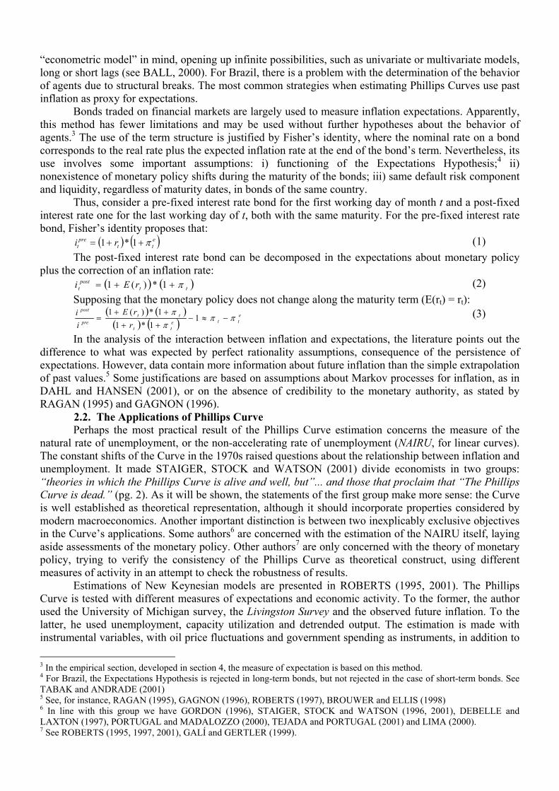
Bonds traded on financial markets are largely used to measure inflation expectations. Apparently, this method has fewer limitations and may be used without further hypotheses about the behavior of agents.3 The use of the term structure is justified by Fisher’s identity, where the nominal rate on a bond corresponds to the real rate plus the expected inflation rate at the end of the bond’s term. Nevertheless, its use involves some important assumptions: i) functioning of the Expectations Hypothesis;4 ii) nonexistence of monetary policy shifts during the maturity of the bonds; iii) same default risk component and liquidity, regardless of maturity dates, in bonds of the same country.

Thus, consider a pre-fixed interest rate bond for the first working day of month t and a post-fixed interest rate one for the last working day of t, both with the same maturity. For the pre-fixed interest rate bond, Fisher’s identity proposes that:

( ) ( )ett

pret ri π++= 1*1 (1)

The post-fixed interest rate bond can be decomposed in the expectations about monetary policy plus the correction of an inflation rate:

( ) ( ttpost

t rEi π++= 1*)(1 ) (2) Supposing that the monetary policy does not change along the maturity term (E(rt) = rt):

( ) ( )( ) ( )

ette

tt

ttpre

post

rrE

ii ππ

ππ

−≈−++

++= 1

1*11*)(1 (3)

In the analysis of the interaction between inflation and expectations, the literature points out the difference to what was expected by perfect rationality assumptions, consequence of the persistence of expectations. However, data contain more information about future inflation than the simple extrapolation of past values.5 Some justifications are based on assumptions about Markov processes for inflation, as in DAHL and HANSEN (2001), or on the absence of credibility to the monetary authority, as stated by RAGAN (1995) and GAGNON (1996).

2.2. The Applications of Phillips Curve Perhaps the most practical result of the Phillips Curve estimation concerns the measure of the

natural rate of unemployment, or the non-accelerating rate of unemployment (NAIRU, for linear curves). The constant shifts of the Curve in the 1970s raised questions about the relationship between inflation and unemployment. It made STAIGER, STOCK and WATSON (2001) divide economists in two groups: “theories in which the Phillips Curve is alive and well, but”... and those that proclaim that “The Phillips Curve is dead.” (pg. 2). As it will be shown, the statements of the first group make more sense: the Curve is well established as theoretical representation, although it should incorporate properties considered by modern macroeconomics. Another important distinction is between two inexplicably exclusive objectives in the Curve’s applications. Some authors6 are concerned with the estimation of the NAIRU itself, laying aside assessments of the monetary policy. Other authors7 are only concerned with the theory of monetary policy, trying to verify the consistency of the Phillips Curve as theoretical construct, using different measures of activity in an attempt to check the robustness of results.

Estimations of New Keynesian models are presented in ROBERTS (1995, 2001). The Phillips Curve is tested with different measures of expectations and economic activity. To the former, the author used the University of Michigan survey, the Livingston Survey and the observed future inflation. To the latter, he used unemployment, capacity utilization and detrended output. The estimation is made with instrumental variables, with oil price fluctuations and government spending as instruments, in addition to 3 In the empirical section, developed in section 4, the measure of expectation is based on this method. 4 For Brazil, the Expectations Hypothesis is rejected in long-term bonds, but not rejected in the case of short-term bonds. See TABAK and ANDRADE (2001) 5 See, for instance, RAGAN (1995), GAGNON (1996), ROBERTS (1997), BROUWER and ELLIS (1998) 6 In line with this group we have GORDON (1996), STAIGER, STOCK and WATSON (1996, 2001), DEBELLE and LAXTON (1997), PORTUGAL and MADALOZZO (2000), TEJADA and PORTUGAL (2001) and LIMA (2000). 7 See ROBERTS (1995, 1997, 2001), GALÍ and GERTLER (1999).

a dummy variable with unit value when the US president was a democrat one. The inclusion of additional inflation lags to correct specification problems raises some doubt on the perfect rationality assumption.

In an attempt to incorporate short-term NAIRU properties, some authors use techniques that can identify changes to the excess of demand over the time. GORDON (1996) estimates the traditional Phillips Curve, allowing NAIRU to follow a random walk. The estimated model is as follows:

( )ttt

tttttt

UU

zLcUULbLa

ε

υππ

+=

++−+=

−*

1*

* )()()( (4)

where U*t is the natural rate at t, zt is a vector of control variables, Ut is the unemployment. If variance of the second equation is equal to zero, the model converges to the traditional analysis, with a non-time-varying NAIRU, a rejected hypothesis in the present study. The estimation is made by way of Gaussian maximum likelihood (see HAMILTON (1994)). The measurements are stable in subsamples and have very narrow confidence intervals. The concavity hypothesis is rejected in favor of the linear formulation.

GORDON (1996) is a response to STAIGER, STOCK and WATSON (1996), who presented high confidence intervals (the NAIRU for 1990 would oscillate between 5.16% and 7.24%). Their estimation used the random walk hypothesis for inflation, where expected inflation corresponds to the past one and did not allow the NAIRU to vary, which could be the source of inaccuracy. In spite of this, the authors make it clear that unemployment has considerable power to forecast the inflation rate.

GALÍ and GERTLER (1999) use a combined form of expectations, criticizing the inaccuracy in the determination of the equilibrium under usual measures of activity. A proxy for real marginal cost would be more valid for its correlation with economic activity and no implicit components that need to be estimated. The estimations use the Generalized Moments Method, instruments being the labor income share, output and spread of short and interests rates. The results point to the enhanced importance of rational expectations. However, the weight of adaptive formation should not be neglected in function of the accuracy of the estimation.

STAIGER, STOCK and WATSON (2001) conducted a new study, with time-varying intercept estimated by the Kalman Filter, in an attempt to estimate NAIRU changes. The model is the same as in GORDON (1996), but it is the constant that varies, not the measure of economic activity. The results accept the validity of the Curve. Yet, it is stressed that movements of wages, prices and unemployment should focus on understanding the univariate trends, because of the instability of parameters over time.

For Brazil, three studies are of note due to their methodology. PORTUGAL and MADALOZZO (2000) use two processes for calculating the NAIRU. The first one is based on the transfer function from a Phillips Curve. Assuming that mistakes are highly costly, the authors use an ARIMA forecasting as expectations. The second method is the estimation of structural components of unemployment. The objective is to eliminate short-term determinants, having the remaining forecast as measure of the NAIRU. The authors reject this methodology, since it did not allow a residual for economic activity that explains the dynamics of inflation.

TEJADA and PORTUGAL (2001), through a time-varying parameter model, allow the convexity of the curve, similarly to DEBELLE and LAXTON (1997). The estimations seem to be more consistent than those in PORTUGAL and MADALOZZO (2000), since they allow lower variance of the NAIRU over time, which seems to be consistent with the notions of structural unemployment.

LIMA (2000) is, technically, the most complex study. The sophistication is justified by the instability of Brazil’s economy in the last years. Two models are estimated: one uses ARCH residuals in the mean equation and the other adds Markov switching to the variance. The author takes past inflation as expectation, using the variation of inflation rate as an endogenous variable. Notably, even using advanced procedures, the statistics on forecast errors and the confidence intervals do not yield satisfactory results.

3. The Phillips Curve Theory and Econometric Methodology The modern version of the Phillips Curve combines the foundation of individual behavior and the

relationships between the economic aggregates into the same theoretical framework, attempting to justify the presence of nominal price rigidity and inflation inertia in the agents’ choices. Assuming models based on staggered contracts (TAYLOR, 1980), we derive the Phillips Curve based on ROBERTS (1997).8 8 It is possible to prove that the model developed by CALVO (1983) produces the same set of equations as a result. For demonstrations, see WALSH (2000), pages 218-220.

Afterwards, we show the compatibility of the sticky inflation model with rational expectations (FUHRER and MOORE, 1995), with the sticky price model, in addition to the relaxation of the expectations hypothesis, as proposed by ROBERTS (1997).

TAYLOR (1980) assumes two-period duration contracts. The mean wage paid by firms is: w (5) ( 2/1−+= ttt xx )Considering that workers are concerned with a measure of demand (e.g. unemployment) and that

pt is the price level at t, we have as job offer: ( )

tt

ett

t Ukppx εα +−=+

− +

21 , (6)

Assuming firms in monopolistic competition, a normalized wage markup to zero is supposed (pt = wt). Combining this with (5) and (6) and defining πt = pt – pt-1, inflation rate at t:

( ) ( ) )(224 111 tErrorUUk ttttett −+++−=− −−+ εεαππ , (7)

where Error(t) = πt - πte defines an expectation error for the current inflation.9 Except for Error(t),

this is the Curve equivalent to the traditional formulation. Hereinafter, Error(t) will be defined as ex-post bias, as in DAHL and HANSEN (2001), to distinguish it from statistical forecast error. The ex-post bias reflects the attributed probability to the regime switch of inflation between t-1 and t, assuming that it follows a Markov process. For the authors, the agents know the current regime only during the transition period. Therefore, attributing a probability other than zero for regime switch causes a bias in expectations.

FUHRER and MOORE (1995) change equation (6), by supposing that workers do not perceive the real wage levels, but the variations of real wages obtained in the previous period. The equation becomes:

( ) ( ) ( ) , (8) 1111 ''2 tt

etttt

tt Ukpxpx

px εα +−+−+−

=− ++−−

Note that real wage is the mean between real wages in the previous period and the expectations for the end of the contract, adjusted according to the economic activity. Therefore, considering the price markup and combining equations (8) with (5):

( ) ( ) )(2'2'4 ,1

,11 tErrorUUk tttt

ett −+++−=∆−∆ −−+ εεαππ , (9)

which is the same equation (7) above, but with variation of inflation and expectations as endogenous variable. ROBERTS (1997) rewrites equation (9) as follows:

( ) ( ) ( )2

)(2

'2'

2,

1,111 tErrorUUk

tttt

ett

t −+++

−=+

− −−+− εεαπππ (10)

The left-hand side is modified to provide an error in inflation forecast, so that part of the equation consists of rational expectations and the remaining of past extrapolation. Thus, FUHRER and MOORE (1995) include in their model both the sticky inflation, with rational expectations, and the sticky price formulation, with agents of different expectation formations. Interestingly, the endogenous variable in (10) does not express a “forecast error”, as ROBERTS (1997) suggests. Its best definition may be the difference between inflation and state of expectations, as “average expectation” is actually formed by past values and the future expectation. Even considering agents with different expectation formations, nothing assures the same proportion. Thus, the sense ascribed may be more appropriate as ex-post bias.

Despite the consensus, some topics are unclear in empirical investigation and in theory implied by the Phillips Curve. Two aspects criticized are inflation inertia and the economy’s behavior in disinflation. According to FUHRER and MOORE (1995), the inertia in TAYLOR (1980) is restricted to the adjustment period of output to equilibrium, which is lower than verified.10 BALL (1994, 1995) shows the chance of economic growth as result of credible deflations. MANKIW and REIS (2001) cite the “flexibility of expectations” to justify their result. GALÍ and GERTLER (1999) show that the model assumes positive correlation between the variation of contemporaneous inflation and the output gap in the future. However, empirical data show an inverse pattern.

FUHRER and MOORE (1995) is one of the variations that tries to correct original problems. Others (ROBERTS, 1997 and 1998, BALL, 2000) make inferences about expectations. BONOMO, 9 Apparently, the error would be in the price level. However, by adding and subtracting the price level at t, we obtain the rate of inflation subtracted from the expected rate - hence, the forecast error. 10 ERCEG and LEVIN (2001) cite studies where inflation persistence coincides with unstable policies. CATI, GARCIA and PERRON (1995) find a random walk of the Brazilian inflation in the period that preceded the Real Plan.

CARRASCO and MOREIRA (2000) include notions of evolutionary games. In cases of disinflations, regardless of credibility, agents choose between adjusting prices and keeping the old strategy. “Myopia” causes losses proportional to the duration of the adaptive strategy. MANKIW and REIS (2001) justify “myopia” by the amount of information the agents receive, since there are costs to improve estimation of inflation. For Brazil, ALMEIDA, MOREIRA and PINHEIRO (2002) replicate ROBERTS (1997), finding evidence in favor of FUHRER and MOORE (1995). One could criticize their sample (from 1990 to 1999), since the two-stage estimator (2SLS) has only asymptotic consistency. Besides, there is no inference about expectations at all, imposing the future value as the agents’ expectations.

3.1. Asymmetry of Prices and Supply Shocks: Controlling exogenous supply shocks is left as a complement imposed by the researcher. The

classical approach uses a set of relatively inelastic supply products. After choosing the set, two options are available: to remove the products from the price index (forming a “core”), or to include the variations as explanation for the model. Adding lags to the equation shows the spread of shock from a sector to the whole economy. The classical control is criticized since it assumes that few sectors have sharp variations in their price level. On the other hand, series that contain most of price index components forms quite a narrow core of variation. Thus, BALL and MANKIW (1995) suggest the use of higher statistical moments of cross-sectional inflation distribution. Asymmetry is justified in models where firms under menu costs only update their prices with the shocks if their profit is higher than the costs. They confirm the presence of enhanced asymmetry component in the US inflation, with loss of significance of the basket of products when the asymmetry and kurtosis variables are added.

MIO (2001) uses the asymmetry of Japanese data and confirms the hypothesis above about the efficiency of this control. The author relates inflation inertia to the asymmetry of the distribution, affirming that the persistent price fluctuations are only due to the spread of shocks, without an “autonomous” inertial component. The author’s measure of asymmetry has interesting properties, as it consists of the difference between the headline and the trimmed inflation:

∑

∑∑

=

=

=

−=−=M

jjt

M

jjtjtN

iitittttSKEW

1

1

1

%30

ω

πωπωππ

(12)

where πt30% is the inflation rate trimmed at 30% on each tail, ωit is the weight of item i in period t, N is the

number of items that form the total price index and M is the number that remains after exclusion.11 The result is the sum of the extreme components of the distribution representing a measure of asymmetry. This measure captures two aspects regarding supply shocks: the shock itself (the more asymmetric the distribution, the more sectors will be in extreme situations), and its persistence. It is also underscored that the variable controls components of IPCA (extended CPI) on a regular basis, such as seasonality. In fact, BALL and MANKIW (1995) and MIO (2001) use full-price indexes and do not control the regressions made with seasonal factors. The measures of elevated statistical moments accomplish this task.

F IG U R E A - C ro s s -S e c tio n a l In fla tio n D is trib u tio n - M a rc h 1 9 9 9

0

2

4

6

8

1 0

1 2

1 4

-3.6

-0.9

-0.4

-0.2 0

0.01

0.22

0.29

0.43

0.56

0.67

0.98 1.5

1.57

1.64

1.88

2.34 2.5

3.35

4.37

4.55 5.4

5.79

6.29

7.24

C a te g o rie s o f IP C A (% )

Cat

egor

ies'

Wei

ghts

T r im m e d T a il: 3 0 %T rim m e d T a il: 3 0 %

T rim m e d IP C A - 0 ,4 3 %

H e a d lin e IP C A - 1 ,1 %

Abrupt changes in relative prices, a special kind of supply shock, can be controlled by the SKEW

variable. Figure A shows the distribution of 47 items of IPCA in March 1999. The black bars show the 11 The choice of the mean with 40% of the core of IPCA is based on FIGUEIREDO (2001). The author points out that this cut tends to value the effects of asymmetry, which is the measure desired as control variable for Brazil.

headline IPCA (1.1%) and the 30% trimmed mean (0.43%). Their large difference is due to the distribution of extreme price variations. It is worth noting that, in March 1999, Brazil experienced the worst moment of the currency crises started in January that year. The exchange rate devaluation had more significant impact on prices of tradable goods, therefore introducing large asymmetry in inflation index.

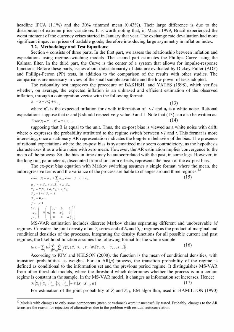
3.2. Methodology and Test Equations: Section 4 consists of three parts. In the first part, we assess the relationship between inflation and

expectations using regime-switching models. The second part estimates the Phillips Curve using the Kalman filter. In the third part, the Curve is the center of a system that allows for impulse-response functions. Before these parts, issues about the stationarity of data are evaluated by Dickey-Fuller (ADF) and Phillips-Perron (PP) tests, in addition to the comparison of the results with other studies. The comparisons are necessary in view of the small sample available and the low power of tests adopted.

The rationality test improves the procedure of BAKHSHI and YATES (1998), which verifies whether, on average, the expected inflation is an unbiased and efficient estimation of the observed inflation, through a cointegration vector with the following format:

tett u+βπ+α=π , (13)

where πet is the expected inflation for t with information of t-1 and ut is a white noise. Rational

expectations suppose that α and β should respectively value 0 and 1. Note that (13) can also be written as: t

ett utError +=−= αππ)( , (14)

supposing that β is equal to the unit. Thus, the ex-post bias is viewed as a white noise with drift, where α expresses the probability attributed to the regime switch between t-1 and t. This format is more interesting, once a stationary AR representation indicates the long-term behavior of the bias. The presence of rational expectations where the ex-post bias is systematized may seem contradictory, as the hypothesis characterizes it as a white noise with zero mean. However, the AR estimation implies convergence to the mean of the process. So, the bias in time t may be autocorrelated with the past, in some lags. However, in the long run, parameter α, discounted from short-term effects, represents the mean of the ex-post bias.

The ex-post bias equation with Markov switching assumes a single format, where the mean, the autoregressive terms and the variance of the process are liable to changes around three regimes:12

=

=

=⇔=++=

++=

+−+= ∑=

23

22

21

3

2

1

332211

332211

0,

000000

,0~

3,2,1

..,0

1

)()(

σσ

σ

θθθθµµµµ

θµ

Nuuu

j

ccS

jSSSSS

SSS

uitErrortError

t

t

t

jt

tjt

tttSt

tttSt

St

k

iStiSt

(15)

MS-VAR estimation includes discrete Markov chains separating different and unobservable M regimes. Consider the joint density of an Yt series and of St and St-1 regimes as the product of marginal and conditional densities of the processes. Integrating the density functions for all possible current and past regimes, the likelihood function assumes the following format for the whole sample:

( ) [∑ ∑ ∑= = =−

−−−−−

=T

t

M

St

M

Sttttttttt SYSSYSSYfL

1 0 0111111 ,|,Pr,,|lnln ] (16)

According to KIM and NELSON (2000), the function is the mean of conditional densities, with transition probabilities as weights. For an AR(p) process, the transition probability of the regime is defined as conditional to the information set and the previous period regime. It distinguishes MS-VAR from other threshold models, where the threshold which determines whether the process is in a certain regime is constant in the sample. In the MS-VAR model, it changes as information set increases. Hence:

{ } { }( ) ( β,|Pr,|Pr 111 −∞

=−∞

=− = ttjjtjjtt SSYSS )

(17)

For estimation of the joint probability of St and St-1, EM algorithm, used in HAMILTON (1990)

12 Models with changes to only some components (mean or variance) were unsuccessfully tested. Probably, changes to the AR terms are the reason for rejection of alternatives due to the problem with residual autocorrelation.

for unobservable regimes, is similar to the Kalman filter, and consists of two steps. In the forecast, the algorithm derives the transition probability given the set of information on the past:

Pr[St = j , St-1 = i | Yt-1 , St-1] = Pr[St = j | St-1 = i].Pr[St-1 = i | Yt-1 , St-1] (18) The first term on the right-hand side is the transition probability, whereas the second is the

transition probability in the previous period. In updating process, the probabilities’ forecast error is incorporated for future steps. So, the filter obtains two types of probability: the smoothed one, containing all information on the sample, and the filtered one, using the available information up to the time of estimation.

The estimation of the Phillips Curve is carried out according to DEBELLE and LAXTON (1997). Developing (10) together with the control variables, we have:

( ) tttt

tttett SELICSKEW

uNAIRU εββγγπααππ +∆++−++= − 211

1.** (19)

Therefore, the constant represents the fixed γ parameter that weights the unobservable component γ*. The variable used to measure economic activity is therefore the inverse of the unemployment, while the NAIRU is the result of the ratio between the negative of γ* and γ. This equation’s format assumes strict convexity in the inflation-unemployment plane.

The assignment of initial values to the filter requires some care, due to the convergence of the algorithm to obtain better values. Here, the estimation by OLS is adopted as initial values, since it provides good rate of convergence, even under regime switching in data. The correction is made using the first k observations only, where k corresponds to the number of parameters in the observation equation.13

The system estimated in the last part of section 4 uses Zellner’s method, estimated by Full-Information Maximum Likelihood (FIML), for correction of the elevated correlation between the residuals of different equations. VAR estimation, which is traditional in the area, was abandoned because of this problem and of the use of a different set of variables in inflation equation.

4. A New Keynesian Phillips Curve for Brazil 4.1. Preliminary Considerations: Stationarity In Brazil, the analysis of stationarity is important in view of the presence of structural breaks in

the economy and their influence on the behavior of variables. Thus, unit root tests should take into consideration its low power, in addition to information obtained from other articles in the field. The presence of a significant break in July 1994 (Real Plan) leads us to adopt the PP test, since the ADF test has lower statistical power.14 The reduced power of the unit root tests also made us avoid their use in sample partitions, given the compromise of the assessed results.

Seven variables are used in the study: IPCA of IBGE, basic index for the inflation targeting system; the expectations derived from interest rates (EXPEC); the ex-post bias, formed by the difference between these two variables; the changes of primary rate (∆SELIC); the measure of skewness proposed by MIO (2001), SKEW; the open seasonally adjusted unemployment rate, 30 days, of IBGE (U30-Census); and the growth rate of monetary stock M1 seasonally adjusted by Census-X11 (M1-Census).

We verify that, differently from CATI, GARCIA and PERRON (1995), the IPCA and EXPEC variables have unit roots in the ADF test. The response given by the test is possibly a consequence of the small sample. Estimating the Phillips Curve, the absence of stationarity would cause damage if there were no cointegration between the variables. However, tests point to the existence of more than one cointegration vector.15 In case of the system of equations, consider the observation of HAMILTON (1994) about systems with nonstationary series, where the use of series in difference would throw away long-term information of the data.16

13 The availability of data from 1990 onwards makes the initial variance increase due to Collor I Plan. Thus, the sample itself behaves like the use of a diffuse Bayesian prior for initial values. 14 Alternative tests, as in CATI, GARCIA and PERRON (1995), were not performed as they were not the aim of this study. However, their conclusions, from other articles, are essential to characterize the dynamics of the variables. 15 Result available from authors. 16 About the use of systems in difference, the author states: “The drawback to this approach is that the true process may not be a VAR in differences. Some of the series may in fact have been stationary, or perhaps some linear combinations of the series are stationary, as in a cointegrated VAR. In such circumstances a VAR in differenced form is misspecified”(page 652).

Results leave no doubt about the ex-post bias. SKEW, M1-Census and SELIC variables have the same behavior as that of inflation and expectations. The ADF test accepts the unit root hypothesis, whereas the PP test points to stationarity. However, the variable for control of the monetary policy is the first difference of SELIC. Thus, as ∆SELIC was stationary, we do not have problems with estimation. In contrast, the PP test shows high chances of stationarity of the SKEW variable and M1 growth. Moreover, the ADF test points to its stationarity at 10%. Thus, the hypotheses of stationarity for SELIC variations and for asymmetry are not a strong restriction to estimation. The evidence of PASTORE (1995) regarding the cointegration between rate of inflation and money stock growth sets argument.

The test on unemployment does not reject the unit root hypothesis. This result is not usual in empirical literature, even when logit transformation is applied to limited variables.17 Probably, this result represents small samples, since tests with significantly larger ones do not endorse the result.

4.2. Analysis of expectations The data on the “expected inflation” variable are available at the site of the Central Bank of Brazil.

The observations consist of nominal yield of pre-fixed CDB (bank deposit certificate) and the post-fixed yield negotiated, respectively, on the first and on the last day of each month, for the number of working days in the month. Information covers the periods from January 1990 to August 2002. Data on the post-fixed CDB consist only of real interest rate. Thus, the spread between the rates expresses the expected inflation rate.18 The inflation used to form the ex-post bias is the IPCA, of IBGE.

This composition has implications for events of each month. Therefore, we have: i) beginning of t: agents have information about t-1; ii) agents form expectations about t from available information; iii) information on t is made available; iv) the agents adapt to information; v) beginning of t+1. Note that agents form their expectations within the same period. The assumption is not very strong, given the lag between collection and dissemination of economic data.

The estimation of a cointegration vector that relates inflation and expectations, in line with BAKHSHI and YATES (1998) and GRANT and THOMAS (1999), does not reject the hypothesis that angular coefficient equals to one. Thus, we may assume that ex-post bias is a stationary representation. Some procedures are traditional when assessing the existence of alternative regimes. One is the variable’s distribution: a bimodal, or even a fat tail, distribution (see HAMILTON, 1994, p. 687) shows signs of more than one regime. According to table A, the Jarque-Bera test is far from configuring a normal distribution for the data. The asymmetry coefficient justifies this behavior. The evaluation also includes the estimation of a model representing the stochastic process of the series. The selection of an AR(1) is due to the adjustment in terms of information criteria and serial autocorrelation. Stability tests check the presence of regimes. The RESET test points to misspecification of the model at 10% with one nonlinear term. The recursive estimation shows large variance of the constant, implying that the confidence interval, depending on the period of analysis, is quite wide.19

TABLE A – Descriptive statistics – Ex-post bias Mean 0.460734 Median -0.022393 Jarque-Bera 33393.68

Standard deviation 3.827322 Asymmetry 7.312726 Prob. 0.000000 Variance 14.64839 Kurtosis 74.12512

The “J” test of DAVIDSON and MACKINNON (1981) was used to determinate the number of regimes. The models were selected with the aim of checking three components: autoregressive dynamics, regimes and dummy variables for economic plans. The justification for the use of dummy variables in some models is the violation of the monetary policy condition in the period covered by CDBs. It is plausible to support the existence of forecast errors under abrupt disinflation processes. Two variables were adopted: one to cover price-freeze period of Collor II Plan (February to June 1991) and another one in months after switch to Real Plan (July 1994). Both have unit value for the time comprised by the event.

The information criteria point to diverse results: while the SIC points to the MS(2)AR(5)20 model, the AIC converges to MS(3)AR(5)-d1. It is worth noting the rejection of a low number of lags, besides 17 For details, see PORTUGAL and MADALOZZO (2000). 18 Similar applications in SCHOR, BONOMO and PEREIRA (1998). 19 Assuming a 95% interval, the constant varies from –5.77 to 4.90. This interval is unrealistic, especially after the Real Plan. 20 The nomenclature follows KROLZIG (1998): “MS(x)AR(y)” points to the model with “x” regimes and AR structure of “y” lags. “d” shows dummy variables in Collor II and Real Plans, “d1” shows dummy variables only in Collor II Plan.

the need of better control of the dummy variables, since, in most tests, the Real Plan variable was not significant at 5%. Possibly, this is consequence of anticipation of the measures by policymakers, since agents showed no “surprise” when implementing the new currency. Table B reports the results of “J” tests. An interesting result was obtained with MS(3)AR(5), as it excelled its equivalent with a dummy variable for Collor II plan. Nevertheless, this is inconsistent with the information criteria.

TABLE B – “J” Test – Number of Regimes Test Estimated value t statistics Choice

Linear X MS(2)AR(1)-d1 0.636933 3.869482 MS(2)AR(1)-d1Linear X MS(3)AR(5)-d1 1.016563 17.03038 MS(3)AR(5)-d1MS(2)AR(1)-d1 X MS(2)AR(5)-d1 0.975699 10.78761 MS(2)AR(5)-d1MS(2)AR(1)-d1 X MS(3)AR(5)-d1 0.994653 16.22412 MS(3)AR(5)-d1MS(2)AR(5) X MS(3)AR(5) 1.078637 18.15003 MS(3)AR(5)MS(2)AR(5) X MS(3)AR(5)-d1 1.017146 14.79181 MS(3)AR(5)-d1MS(3)AR(5) X MS(3)AR(5)-d1 0.514212* 8.719056* MS(3)AR(5)

NOTE: “Test” reports confronted models, the first of which is a null hypothesis, while the second is the alternative. “Estimated Value” shows estimation of alternative model in the test. “t statistics” informs the significance of the parameter.

The estimation of the model with Markov switching and one control variable (Collor II Plan) yielded the results in table C.21 The test of DAVIES (1977), standard to confirm the presence of more than one regime, shows the acceptance of the Markov model. Residuals do not show autocorrelation. The sensitivity test, however, captures problems, for instance, in the elimination of ARCH-type residuals at 5%. The test is performed with smoothed residuals, trying, as GARCIA and PERRON (1996) did, to capture the presence of regime-dependent changes to the variance. In contrast, according to KIM and NELSON (2000), ARCH-type residuals were not found with the test on standardized residuals.

TABLE C – Estimation of the Regime Switching Model – MS(3)AR(5)-d1 Variable Coefficient (Std. Error) Variable Coefficient (Std. Error)

Regime 1 – Standard Error: 0.13019 C (Regime 1) -0.6891 (0.0507**) AR(4) -0.1302 (0.0134**) AR(1) 0.6424 (0.0150**) AR(5) 0.0359 (0.0191) AR(2) -0.5132 (0.0136**) Collor II -0.6891 (0.0507**) AR(3) 0.0168 (0.0169)

Regime 2 – Standard Error: 0.48182 C (Regime 2) -0.0185 (0.0495) AR(4) -0.0540 (0.0167**) AR(1) 0.5845 (0.0861**) AR(5) 0.1194 (0.0151**) AR(2) -0.0248 (0.0818) Collor II -4.3723 (94.9852) AR(3) 0.0897 (0.0198**)

Regime 3 – Standard Error: 2.1882 C (Regime 3) 1.5081 (0.4551**) AR(4) -0.1276 (0.1615) AR(1) -0.4969 (0.1424**) AR(5) -0.1270 (0.1213) AR(2) -0.0990 (0.1790) Collor II 10.5075 (1.8273**) AR(3) -0.2933 (0.1541*)

Comparison with the Linear Model: log-likelihood: -171.2123 linear system : -292.5500AIC criterion: 2.7376 linear system : 4.0891SC criterion: 3.3479 linear system : 4.2519LR linearity test: 242.6753 Chi(16) =[0.0000] ** Chi(22)=[0.0000] **DAVIES = [0.0000] **

NOTE: (**) / (*) indicates the significance of parameters estimated at 1% / 5%. As shown in graph 1, regimes 2 and 3 determine low and high inflation regimes, respectively.

Regime 2 presents low variance, nonexistence of systematic errors (constant indifferent from zero) and high persistence of ex-post bias. Regime 3 is characterized by underestimation of inflation and high persistence of ex-post bias. Regime 1 captured two peaks between April and June 1991 and July and August 1994. In both cases, periods coincide with expectations that are higher than inflation, either due to hope for the end of the price-freeze at the first peak or due to the credibility regarding the July 1994 plan.

Durability is one more aspect of regime 1. The transition matrix of regimes is given by:

21 All models with Markov switches were estimated by the MS-VAR 1.30 package, written by Hans-Martin Krolzig for use as mentioned in Ox 3.00 software, developed by Jurgen Doornik.

−−=

8154.05062.21846.011540.99884.001159.0

5496.01042.03463.0

EEP

As we may observe, the largest probability, from the moment we enter regime 1, is that agents tend towards the regime with higher variance and high forecast error. We verify that there is a minimally calculated probability of being in regime 1 and remaining in it, with duration of approximately one month and a half, as against a probability of 86 months in period 2. This is directly related to the time interval at which regimes occur: regime 1 was always followed by high inflation periods. The sole exception is the period between July and August 1994, when the economy entered a permanent phase of low inflation.

1991 1992 1993 1994 1995 1996 1997 1998 1999 2000 2001 2002

0.5

1.0Probabilities of Regim e 1

G RAP H 1 - Estim ated P robabilities - M S(3)AR(5)-d1

filt ered p redic t ed

sm o o t h ed

1991 1992 1993 1994 1995 1996 1997 1998 1999 2000 2001 2002

0.5

1.0Probabilities of Regim e 2

1991 1992 1993 1994 1995 1996 1997 1998 1999 2000 2001 2002

0.5

1.0Probabilities of Regim e 3

The conditional duration’s probability, which conveys the notion of trajectory between regimes

over time, is shown in graph 2. It confirms that when economy enters regime 1, it tends to cause high inflation. However, in the long run, the permanence in high inflation is not supported, thus causing the economy to switch to a regime with lower volatility. According to the maxim of chronic cases of inflation, it is confirmed that “every hyperinflation has an end in itself.”

0 5 1 0 1 5 2 0 2 5 3 0 3 5 4 0 4 5 5 0 5 5 6 0 6 5 7 0

0 .5

1 .0P r e d ic te d h - s te p p r o b a b ilitie s w h e n s t = 1

G R A P H 2 - C o n d ic io n a l D u ra t io n 's P ro b a b ilit ie s - M S (3 )A R (5 )-d 1R e g i m e 1 R e g i m e 3

R e g i m e 2

0 5 1 0 1 5 2 0 2 5 3 0 3 5 4 0 4 5 5 0 5 5 6 0 6 5 7 0

0 .5

1 .0 P r e d ic te d h - s te p p r o b a b ilitie s w h e n s t = 2

0 5 1 0 1 5 2 0 2 5 3 0 3 5 4 0 4 5 5 0 5 5 6 0 6 5 7 0

0 .5

1 .0P r e d ic te d h - s te p p r o b a b ilitie s w h e n s t = 3

Therefore, three aspects should be considered in estimations of the Phillips Curve for Brazil. The

first concerns the fact that the perception about the Brazilian economy by the agents moves between well-defined regimes, characterized by the volatility of inflation and by the persistence of the agents’ behavior. Secondly, the transition between regimes also has characteristics that relate to the economic policy environment. Thus, the way the economic policy is exposed by the government is important to expectation formations. Finally, the estimation of functions such as the Phillips Curve should consider some type of nonlinearity. FERRI, GREENBERG and DAY (2001) observe that these forms may interfere with the estimation in either three ways: by changing the relationship between expectations and inflation, the relationship between inflation and excess demand, and the relationship between inflation and exogenous factors. Here, the relationship will be exogenously imposed on the model, by the selection of the strictly convex form in the inflation-unemployment tradeoff. Nevertheless, as will be discussed, this format has a close link with the Markov model presented.

4.3. Estimate: a short-term NAIRU for Brazil The results of the estimation are presented in table D. The convex format assumes increasing costs

in terms of unemployment so that lower inflation rates can be obtained. Comparatively, there are increasing costs in terms of inflation, which correspond to lower rates of unemployment. All coefficients are significant and the “t” statistics for sum of expectation coefficients does not reject the hypothesis of the sum equal to the unit.22 The high value of R2 statistics is satisfactory when the variance matrix is estimated at each time point.23 There are no signs of residual autocorrelation.

TABLE D –Phillips Curve Estimation – January/90 to August/02 Coefficient Std. deviation t statistics Prob. γ -8.735281 1.411316 -6.189460 0.0000α 0.749142 0.045299 16.53755 0.0000α∗ 0.218704 0.057766 3.786036 0.0002β1 0.885852 0.149229 5.936188 0.0000β2 0.092981 0.041562 2.237145 0.0269

Final γ* 73.93179 2.884639 25.62948 0.0000Variance of Measurement Equation 2.277436 0.249294 9.135558 0.0000

Variance of State Equation 15.06066 7.658521 1.966523 0.0513Maximum [abs(∆u*)]: -0.97405 (March/91) Maximum [u*t-ut]: 2.02409 (August/90)Log Likelihood -294.8187

( )

t1tt

tt2t1t

ttt1t

ett

**

SELICSKEWu

uNAIRU**

υ+γ=γ

ε+∆β+β+γ−γ

+πα+απ=π

−

−

R-squared 0.988737 Durbin-Watson stat 2.234003S.E. of regression 1.371114 Sum squared resid 263.1936The significance of the changes in the SELIC rate is noteworthy as it serves as an explanatory

factor for the rate of inflation. If changes to the monetary policy were accurately forecasted, the information would be contained in the spread of interest rates, rendering variations in the primary rate insignificant to the contemporaneous behavior of inflation. Thus, the use of ∆SELIC as an instrument is decisive for maintaining the policy on the maturity date of the negotiated bonds.

GRAPH 3 - Unemployment and Smoothed NAIRU - Aug/90 to Aug/02

4

5

6

7

8

9

08/1

990

02/1

991

08/1

991

02/1

992

08/1

992

02/1

993

08/1

993

02/1

994

08/1

994

02/1

995

08/1

995

02/1

996

08/1

996

02/1

997

08/1

997

02/1

998

08/1

998

02/1

999

08/1

999

02/2

000

08/2

000

02/2

001

08/2

001

02/2

002

08/2

002

Period

(%)

Unemployment NAIRU-SM By assessing the variance of the state equation, it is noted that the NAIRU changes over time, with

a significance of 10%. The greatest variation was of almost one percentage point, registered right after the implementation of Collor II Plan (February 1991). Conversely, the largest unemployment gap (“NAIRU gap”) was registered during the recession caused by Collor I Plan. The behavior of the natural rate does not imply inaccuracy of estimations. Graph 3 shows unemployment, the smoothed NAIRU and the 95% confidence intervals for the estimation.24 Comparing with results for the US, where STAIGER, STOCK and WATSON (1996) obtained a 1.8% interval, the maximum interval (close to 0.8%, with a 95%CI) 22 It was not possible to perform the LR test due to the absence of algorithm convergence to the calculation of likelihood of the alternative model. 23 Equivalent estimations that did not allow changes to the variance matrix presented problems with serial autocorrelation, despite the higher stability of the estimated NAIRU, both in the filtered and smoothed series. 24 The standard deviation of the estimation was calculated by imposing restrictions on the fixed coefficients of the equation. Thus, the standard deviation for the variable coefficient only indicates the inaccuracy of the NAIRU estimation.

indicates a good NAIRU estimation. We can assess the capacity of the model to adjust the excess demand to variations in inflation.

Graph 4 relates the deviations of inflation from the expectation component (πt - απet – (1-α)πt-1)) with

excess demand (γ(u*t – ut)/ut). It is possible to divide the period into three different phases: pre-Real Plan, first phase of the Real Plan and the post-1999 period. In the high inflation period, there was strong demand, which systematically made unemployment fall below the NAIRU, dissociated from inflation expectations, whose value was less than the observed. Exceptions are found after the implementation of Collor II Plan and between last quarter of 1991 and the end of first quarter of 1992, which characterizes the economic slowdown during the term of Mr. Marcílio Marques Moreira as Minister of Finance.

GRAPH 4 - Historical Performance - Non-Linear Phillips Curve - Aug/90 to Aug/02

-10

0

10

20

08/1

990

02/1

991

08/1

991

02/1

992

08/1

992

02/1

993

08/1

993

02/1

994

08/1

994

02/1

995

08/1

995

02/1

996

08/1

996

02/1

997

08/1

997

02/1

998

08/1

998

02/1

999

08/1

999

02/2

000

08/2

000

02/2

001

08/2

001

02/2

002

08/2

002

Period

Labo

r Mar

ket (

%)

-6

-3

0

3

6

9

12

15

Inflation's Forecast Errors (%)

Labor Market Pressure Inflation's Forecast Errors During the first phase of the Real plan, unemployment was always above the NAIRU, as a result

of measures that aimed at holding back the aggregate demand. The use of high real interest rates combined with a series of external shocks (namely, Mexico, 95, Asia, 97, Russia, 98) retracted the economic activity, cushioning a new rise in inflation. Graph 4 shows frequent overestimations of the inflation rate and the pressure for deflation observed in the market. After the depreciation of Real, in January 1999, the measure of excess demand takes on some kind of threshold between inflation control and economic growth. Between 1999 and 2001, the negative inflation surprises are corroborated by the higher pressure for aggregate demand on the prices. It is possible to observe two points of pressure for demand on the rates of inflation, seen in the first semester of 2001 and in the first semester of 2002.

The skewness variable proposed by MIO (2001) is significant in the model. The estimation implies that changes of one percentage point from the rate of inflation in relation to its core produce variations of 0.88 percentage points in inflation. To test for inertia, MIO (2001) proposes that by removing the skewness from both sides of the function, the Curve may be modeled in an equivalent form by “core inflation.” For that, it is necessary that: i) the SKEW coefficient in t is indifferent from unit; and, ii) skewness lagged coefficients be symmetric to those of the lagged inflation. The LR test performed25 rejects these hypotheses (LR = 27.21, for chi-square with two degrees of freedom), and allows us to state that the supply shocks are not responsible for the totality of the inertial component in the analyzed period, with an autonomous response of inflation to shocks.

It may seem surprising to argue that the rise in inflation after the devaluation of the Real, in 1999, was caused by a fall in the NAIRU gap, once there was a strong cost pressure on prices. However, Figure A shows that the SKEW variable captures relative price changes (price asymmetry) caused by a temporary shock over a few sectors of the economy (tradable goods). Thus, at least part of the exchange rate variation was removed from the estimated implicit component. The fall in the NAIRU gap could therefore not be caused by a model’s misspecification that excluded the exchange rate.

Three robustness tests were performed with the estimated model. The first consists of the comparison of the values for the expectations coefficients in models with different measures of activity. The results showed coefficients with fewer oscillations, even when seasonal components are included.26 25 Models used here are available from authors. Note that comparison in this test should not be made on the standard model, as this type of model does not employ lags of the SKEW variable. 26 Alternative estimations available from authors.

In general, tests reject the hypothesis that the sum of expectations coefficients is equal to the unit. The second test is the “J” test to verify control variables, the seasonal factor of unemployment and

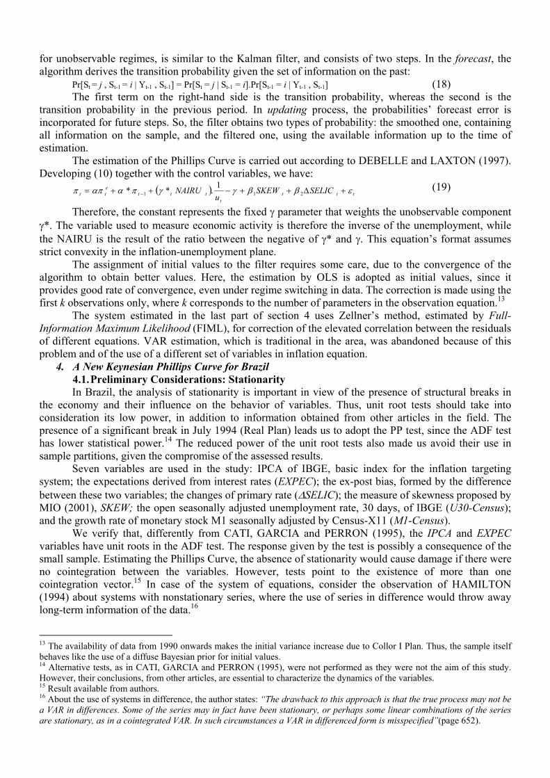
the convexity of the Curve. In the first two cases, the standard model has clear advantage over the alternative, including a model estimated with only adaptive expectations. Conversely, the comparison with the linear model led to inconclusive results. In fact, the latter has good data adjustment, almost equivalent to the standard model, if we observe the R2 of both regressions. What sharply distinguishes it is the estimated NAIRU’s confidence interval, shown in Graph 5 together with the standard NAIRU.

GRAPH 5 - Comparison of Estimates - Convex and Linear NAIRU

3

4

5

6

7

8

9

1008

/199

0

02/1

991

08/1

991

02/1

992

08/1

992

02/1

993

08/1

993

02/1

994

08/1

994

02/1

995

08/1

995

02/1

996

08/1

996

02/1

997

08/1

997

02/1

998

08/1

998

02/1

999

08/1

999

02/2

000

08/2

000

02/2

001

08/2

001

02/2

002

08/2

002

Period

(%)

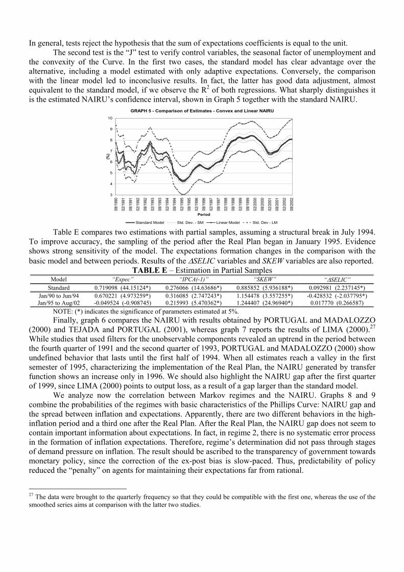
Standard Model Std. Dev. - SM Linear Model Std. Dev - LM Table E compares two estimations with partial samples, assuming a structural break in July 1994.

To improve accuracy, the sampling of the period after the Real Plan began in January 1995. Evidence shows strong sensitivity of the model. The expectations formation changes in the comparison with the basic model and between periods. Results of the ∆SELIC variables and SKEW variables are also reported.

TABLE E – Estimation in Partial Samples Model “Expec” “IPCA(-1)” “SKEW” “∆SELIC”

Standard 0.719098 (44.15124*) 0.276066 (14.63686*) 0.885852 (5.936188*) 0.092981 (2.237145*) Jan/90 to Jun/94 0.670221 (4.973259*) 0.316085 (2.747243*) 1.154478 (3.557255*) -0.428532 (-2.037795*) Jan/95 to Aug/02 -0.049524 (-0.908745) 0.215993 (5.470362*) 1.244407 (24.96940*) 0.017770 (0.266587)

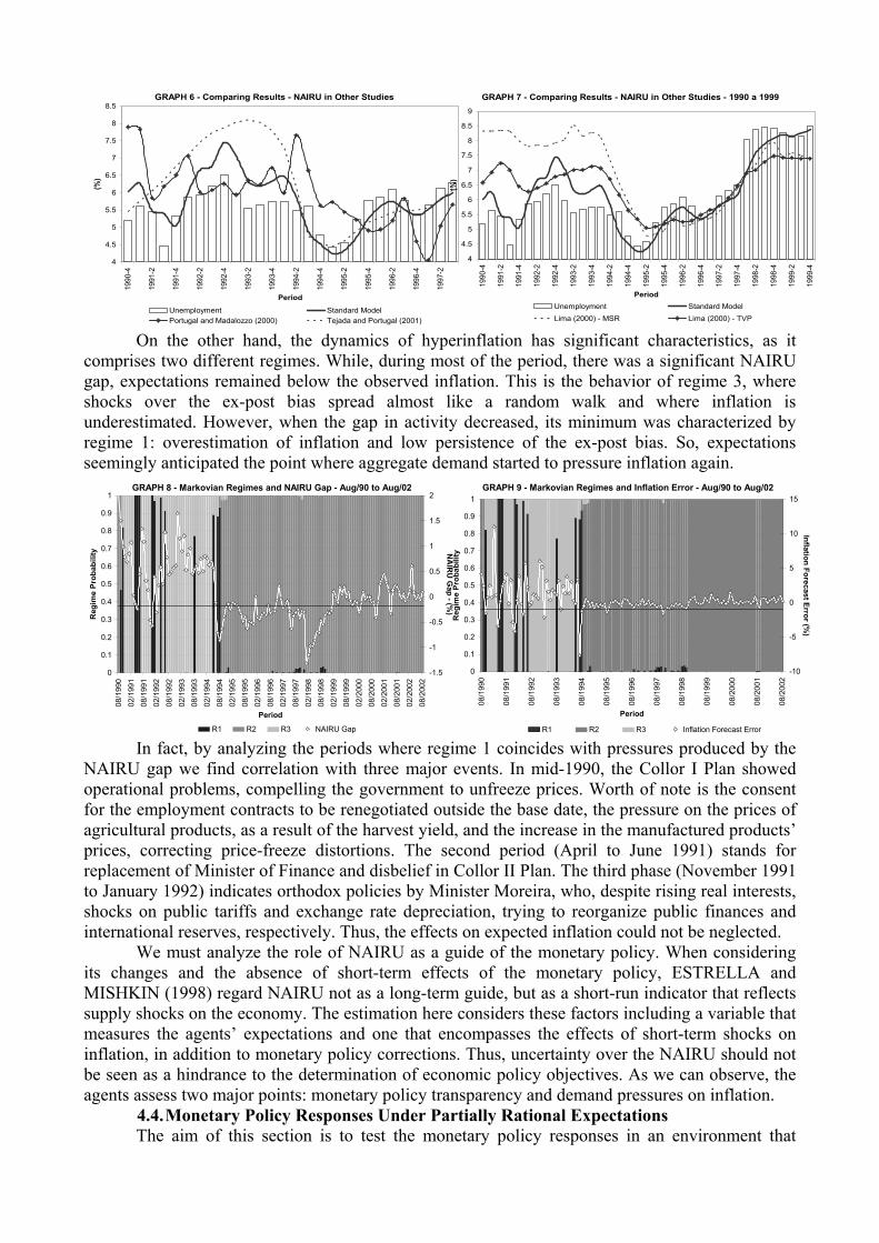
NOTE: (*) indicates the significance of parameters estimated at 5%. Finally, graph 6 compares the NAIRU with results obtained by PORTUGAL and MADALOZZO

(2000) and TEJADA and PORTUGAL (2001), whereas graph 7 reports the results of LIMA (2000).27 While studies that used filters for the unobservable components revealed an uptrend in the period between the fourth quarter of 1991 and the second quarter of 1993, PORTUGAL and MADALOZZO (2000) show undefined behavior that lasts until the first half of 1994. When all estimates reach a valley in the first semester of 1995, characterizing the implementation of the Real Plan, the NAIRU generated by transfer function shows an increase only in 1996. We should also highlight the NAIRU gap after the first quarter of 1999, since LIMA (2000) points to output loss, as a result of a gap larger than the standard model.

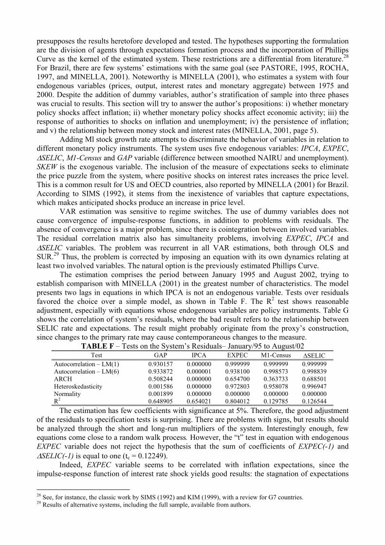
We analyze now the correlation between Markov regimes and the NAIRU. Graphs 8 and 9 combine the probabilities of the regimes with basic characteristics of the Phillips Curve: NAIRU gap and the spread between inflation and expectations. Apparently, there are two different behaviors in the high-inflation period and a third one after the Real Plan. After the Real Plan, the NAIRU gap does not seem to contain important information about expectations. In fact, in regime 2, there is no systematic error process in the formation of inflation expectations. Therefore, regime’s determination did not pass through stages of demand pressure on inflation. The result should be ascribed to the transparency of government towards monetary policy, since the correction of the ex-post bias is slow-paced. Thus, predictability of policy reduced the “penalty” on agents for maintaining their expectations far from rational.

27 The data were brought to the quarterly frequency so that they could be compatible with the first one, whereas the use of the smoothed series aims at comparison with the latter two studies.

GRAPH 6 - Comparing Results - NAIRU in Other Studies

4

4.5

5

5.5

6

6.5

7

7.5

8

8.5

1990

-4

1991

-2

1991

-4

1992

-2

1992

-4

1993

-2

1993

-4

1994

-2

1994

-4

1995

-2

1995

-4

1996

-2

1996

-4

1997

-2

Period

(%)

Unemployment Standard ModelPortugal and Madalozzo (2000) Tejada and Portugal (2001)

GRAPH 7 - Comparing Results - NAIRU in Other Studies - 1990 a 1999

4

4.5

5

5.5

6

6.5

7

7.5

8

8.5

9

1990

-4

1991

-2

1991

-4

1992

-2

1992

-4

1993

-2

1993

-4

1994

-2

1994

-4

1995

-2

1995

-4

1996

-2

1996

-4

1997

-2

1997

-4

1998

-2

1998

-4

1999

-2

1999

-4

Period

(%)

Unemployment Standard ModelLima (2000) - MSR Lima (2000) - TVP

On the other hand, the dynamics of hyperinflation has significant characteristics, as it comprises two different regimes. While, during most of the period, there was a significant NAIRU gap, expectations remained below the observed inflation. This is the behavior of regime 3, where shocks over the ex-post bias spread almost like a random walk and where inflation is underestimated. However, when the gap in activity decreased, its minimum was characterized by regime 1: overestimation of inflation and low persistence of the ex-post bias. So, expectations seemingly anticipated the point where aggregate demand started to pressure inflation again.

GRAPH 8 - Markovian Regimes and NAIRU Gap - Aug/90 to Aug/02

0

0.1

0.2

0.3

0.4

0.5

0.6

0.7

0.8

0.9

1

08/1

990

02/1

991

08/1

991

02/1

992

08/1

992

02/1

993

08/1

993

02/1

994

08/1

994

02/1

995

08/1

995

02/1

996

08/1

996

02/1

997

08/1

997

02/1

998

08/1

998

02/1

999

08/1

999

02/2

000

08/2

000

02/2

001

08/2

001

02/2

002

08/2

002

Period

Reg

ime

Prob

abili

ty

-1.5

-1

-0.5

0

0.5

1

1.5

2

NA

IRU

Gap - (%

)

R1 R2 R3 NAIRU Gap

GRAPH 9 - Markovian Regimes and Inflation Error - Aug/90 to Aug/02

0

0.1

0.2

0.3

0.4

0.5

0.6

0.7

0.8

0.9

1

08/1

990

08/1

991

08/1

992

08/1

993

08/1

994

08/1

995

08/1

996

08/1

997

08/1

998

08/1

999

08/2

000

08/2

001

08/2

002

Period

Reg

ime

Prob

abili

ty

-10

-5

0

5

10

15

Inflation Forecast Error (%)

R1 R2 R3 Inflation Forecast Error In fact, by analyzing the periods where regime 1 coincides with pressures produced by the

NAIRU gap we find correlation with three major events. In mid-1990, the Collor I Plan showed operational problems, compelling the government to unfreeze prices. Worth of note is the consent for the employment contracts to be renegotiated outside the base date, the pressure on the prices of agricultural products, as a result of the harvest yield, and the increase in the manufactured products’ prices, correcting price-freeze distortions. The second period (April to June 1991) stands for replacement of Minister of Finance and disbelief in Collor II Plan. The third phase (November 1991 to January 1992) indicates orthodox policies by Minister Moreira, who, despite rising real interests, shocks on public tariffs and exchange rate depreciation, trying to reorganize public finances and international reserves, respectively. Thus, the effects on expected inflation could not be neglected.

We must analyze the role of NAIRU as a guide of the monetary policy. When considering its changes and the absence of short-term effects of the monetary policy, ESTRELLA and MISHKIN (1998) regard NAIRU not as a long-term guide, but as a short-run indicator that reflects supply shocks on the economy. The estimation here considers these factors including a variable that measures the agents’ expectations and one that encompasses the effects of short-term shocks on inflation, in addition to monetary policy corrections. Thus, uncertainty over the NAIRU should not be seen as a hindrance to the determination of economic policy objectives. As we can observe, the agents assess two major points: monetary policy transparency and demand pressures on inflation.

4.4. Monetary Policy Responses Under Partially Rational Expectations The aim of this section is to test the monetary policy responses in an environment that

presupposes the results heretofore developed and tested. The hypotheses supporting the formulation are the division of agents through expectations formation process and the incorporation of Phillips Curve as the kernel of the estimated system. These restrictions are a differential from literature.28 For Brazil, there are few systems’ estimations with the same goal (see PASTORE, 1995, ROCHA, 1997, and MINELLA, 2001). Noteworthy is MINELLA (2001), who estimates a system with four endogenous variables (prices, output, interest rates and monetary aggregate) between 1975 and 2000. Despite the addition of dummy variables, author’s stratification of sample into three phases was crucial to results. This section will try to answer the author’s propositions: i) whether monetary policy shocks affect inflation; ii) whether monetary policy shocks affect economic activity; iii) the response of authorities to shocks on inflation and unemployment; iv) the persistence of inflation; and v) the relationship between money stock and interest rates (MINELLA, 2001, page 5).

Adding Ml stock growth rate attempts to discriminate the behavior of variables in relation to different monetary policy instruments. The system uses five endogenous variables: IPCA, EXPEC, ∆SELIC, M1-Census and GAP variable (difference between smoothed NAIRU and unemployment). SKEW is the exogenous variable. The inclusion of the measure of expectations seeks to eliminate the price puzzle from the system, where positive shocks on interest rates increases the price level. This is a common result for US and OECD countries, also reported by MINELLA (2001) for Brazil. According to SIMS (1992), it stems from the inexistence of variables that capture expectations, which makes anticipated shocks produce an increase in price level.

VAR estimation was sensitive to regime switches. The use of dummy variables does not cause convergence of impulse-response functions, in addition to problems with residuals. The absence of convergence is a major problem, since there is cointegration between involved variables. The residual correlation matrix also has simultaneity problems, involving EXPEC, IPCA and ∆SELIC variables. The problem was recurrent in all VAR estimations, both through OLS and SUR.29 Thus, the problem is corrected by imposing an equation with its own dynamics relating at least two involved variables. The natural option is the previously estimated Phillips Curve.

The estimation comprises the period between January 1995 and August 2002, trying to establish comparison with MINELLA (2001) in the greatest number of characteristics. The model presents two lags in equations in which IPCA is not an endogenous variable. Tests over residuals favored the choice over a simple model, as shown in Table F. The R2 test shows reasonable adjustment, especially with equations whose endogenous variables are policy instruments. Table G shows the correlation of system’s residuals, where the bad result refers to the relationship between SELIC rate and expectations. The result might probably originate from the proxy’s construction, since changes to the primary rate may cause contemporaneous changes to the measure.

TABLE F – Tests on the System’s Residuals– January/95 to August/02 Test GAP IPCA EXPEC M1-Census ∆SELIC

Autocorrelation – LM(1) 0.930157 0.000000 0.999999 0.999999 0.999999 Autocorrelation – LM(6) 0.933872 0.000001 0.938100 0.998573 0.998839 ARCH 0.508244 0.000000 0.654700 0.363733 0.688501 Heteroskedasticity 0.001586 0.000000 0.972803 0.958078 0.996947 Normality 0.001899 0.000000 0.000000 0.000000 0.000000 R2 0.648905 0.654021 0.804012 0.129785 0.126544

The estimation has few coefficients with significance at 5%. Therefore, the good adjustment of the residuals to specification tests is surprising. There are problems with signs, but results should be analyzed through the short and long-run multipliers of the system. Interestingly enough, few equations come close to a random walk process. However, the “t” test in equation with endogenous EXPEC variable does not reject the hypothesis that the sum of coefficients of EXPEC(-1) and ∆SELIC(-1) is equal to one (tc = 0.12249).

Indeed, EXPEC variable seems to be correlated with inflation expectations, since the impulse-response function of interest rate shock yields good results: the stagnation of expectations

28 See, for instance, the classic work by SIMS (1992) and KIM (1999), with a review for G7 countries. 29 Results of alternative systems, including the full sample, available from authors.

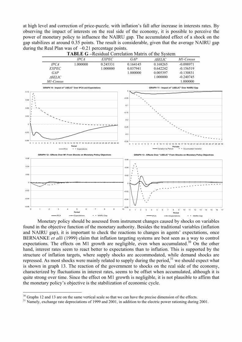
at high level and correction of price-puzzle, with inflation’s fall after increase in interests rates. By observing the impact of interests on the real side of the economy, it is possible to perceive the power of monetary policy to influence the NAIRU gap. The accumulated effect of a shock on the gap stabilizes at around 0.35 points. The result is considerable, given that the average NAIRU gap during the Real Plan was of –0.21 percentage points.

TABLE G –Residual Correlation Matrix of the System IPCA EXPEC GAP ∆SELIC M1-Census

IPCA 1.000000 0.245331 0.164145 0.168265 -0.098971 EXPEC 1.000000 0.037941 0.642242 -0.156519

GAP 1.000000 0.005397 -0.130831 ∆SELIC 1.000000 -0.240745

M1-Census 1.000000

GRAPH 10 - Impact of "∆SELIC" Over IPCA and Expectations

-0.06

-0.03

0

0.03

0.06

0.09

0.12

0 1 2 3 4 5 6 7 8 9 10 11 12 13 14 15 16 17 18 19 20 21 22 23 24 25 26 27 28 29 30

Period

GRAPH 11 - Impact of "∆SELIC" Over NAIRU Gap

-0.35

-0.3

-0.25

-0.2

-0.15

-0.1

-0.05

0

0 1 2 3 4 5 6 7 8 9 10 11 12 13 14 15 16 17 18 19 20 21 22 23 24 25 26 27 28 29 30Período

IPCA Expectations

GRAPH 12 - Effects Over M1 From Shocks on Monetary Policy Objectives

-0.06

-0.04

-0.02

0

0.02

0.04

0.06

0 1 2 3 4 5 6 7 8 9

Period10

GRAPH 13 - Effects Over "∆SELIC" From Shocks on Monetary Policy Objectives

-0.06

-0.04

-0.02

0

0.02

0.04

0.06

0 1 2 3 4 5 6 7 8 9 10 11 12 13 14 15 16 17

PeriodIPCA Expectations NAIRU Gap

Variation by Period Accumulated Variation

IPCA Expectations NAIRU Gap

Monetary policy should be assessed from instrument changes caused by shocks on variables found in the objective function of the monetary authority. Besides the traditional variables (inflation and NAIRU gap), it is important to check the reactions to changes in agents’ expectations, once BERNANKE et alli (1999) claim that inflation targeting systems are best seen as a way to control expectations. The effects on M1 growth are negligible, even when accumulated.30 On the other hand, interest rates seem to react better to expectations than to inflation. This is supported by the structure of inflation targets, where supply shocks are accommodated, while demand shocks are repressed. As most shocks were mainly related to supply during the period,31 we should expect what is shown in graph 13. The reaction of the government to shocks on the real side of the economy, characterized by fluctuations in interest rates, seems to be offset when accumulated, although it is quite strong over time. Since the effect on M1 growth is negligible, it is not plausible to affirm that the monetary policy’s objective is the stabilization of economic cycle.

30 Graphs 12 and 13 are on the same vertical scale so that we can have the precise dimension of the effects. 31 Namely, exchange rate depreciations of 1999 and 2001, in addition to the electric power rationing during 2001.

GRAPH 14 - Effects from Shocks on M1 Over ∆SELIC and from ∆SELIC Over M1

-0.015

-0.010

-0.005

0.000

0.005

0.010

0.015

0.020

0.025

0 1 2 3 4 5 6 7 8 9 10Period

Effe

ct o

ver "

∆SE

LIC"

-0.008

-0.006

-0.004

-0.002

0

0.002

0.004

0.006

0.008

0.01

0.012

0.014

Effects over M1

Effect over "DSELIC" Effect over M1

GRAPH 15 - Inflacionary Persistence

-0.08

-0.06

-0.04

-0.02

0

0.02

0.04

0.06

0.08

0.1

0 1 2 3 4 5 6 7 8 9 10 11 12 13 14 15 16 17 18 19 20 21Period

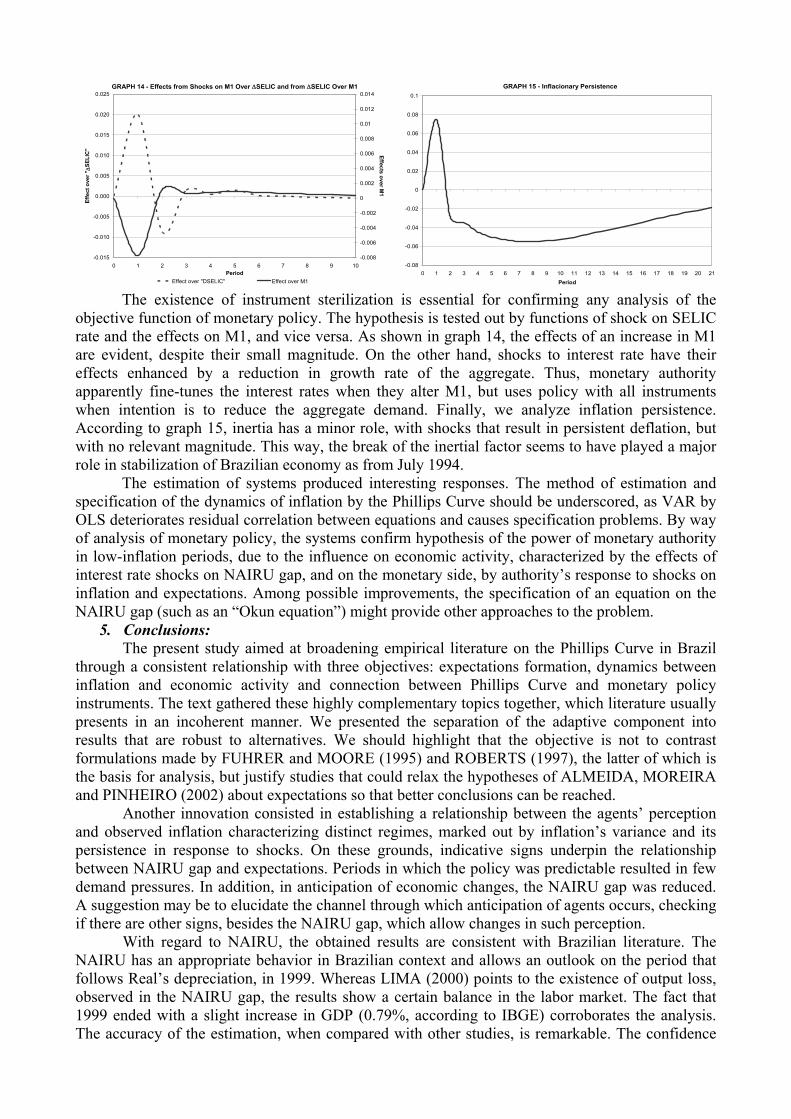
The existence of instrument sterilization is essential for confirming any analysis of the objective function of monetary policy. The hypothesis is tested out by functions of shock on SELIC rate and the effects on M1, and vice versa. As shown in graph 14, the effects of an increase in M1 are evident, despite their small magnitude. On the other hand, shocks to interest rate have their effects enhanced by a reduction in growth rate of the aggregate. Thus, monetary authority apparently fine-tunes the interest rates when they alter M1, but uses policy with all instruments when intention is to reduce the aggregate demand. Finally, we analyze inflation persistence. According to graph 15, inertia has a minor role, with shocks that result in persistent deflation, but with no relevant magnitude. This way, the break of the inertial factor seems to have played a major role in stabilization of Brazilian economy as from July 1994.

The estimation of systems produced interesting responses. The method of estimation and specification of the dynamics of inflation by the Phillips Curve should be underscored, as VAR by OLS deteriorates residual correlation between equations and causes specification problems. By way of analysis of monetary policy, the systems confirm hypothesis of the power of monetary authority in low-inflation periods, due to the influence on economic activity, characterized by the effects of interest rate shocks on NAIRU gap, and on the monetary side, by authority’s response to shocks on inflation and expectations. Among possible improvements, the specification of an equation on the NAIRU gap (such as an “Okun equation”) might provide other approaches to the problem.

5. Conclusions: The present study aimed at broadening empirical literature on the Phillips Curve in Brazil

through a consistent relationship with three objectives: expectations formation, dynamics between inflation and economic activity and connection between Phillips Curve and monetary policy instruments. The text gathered these highly complementary topics together, which literature usually presents in an incoherent manner. We presented the separation of the adaptive component into results that are robust to alternatives. We should highlight that the objective is not to contrast formulations made by FUHRER and MOORE (1995) and ROBERTS (1997), the latter of which is the basis for analysis, but justify studies that could relax the hypotheses of ALMEIDA, MOREIRA and PINHEIRO (2002) about expectations so that better conclusions can be reached.

Another innovation consisted in establishing a relationship between the agents’ perception and observed inflation characterizing distinct regimes, marked out by inflation’s variance and its persistence in response to shocks. On these grounds, indicative signs underpin the relationship between NAIRU gap and expectations. Periods in which the policy was predictable resulted in few demand pressures. In addition, in anticipation of economic changes, the NAIRU gap was reduced. A suggestion may be to elucidate the channel through which anticipation of agents occurs, checking if there are other signs, besides the NAIRU gap, which allow changes in such perception.

With regard to NAIRU, the obtained results are consistent with Brazilian literature. The NAIRU has an appropriate behavior in Brazilian context and allows an outlook on the period that follows Real’s depreciation, in 1999. Whereas LIMA (2000) points to the existence of output loss, observed in the NAIRU gap, the results show a certain balance in the labor market. The fact that 1999 ended with a slight increase in GDP (0.79%, according to IBGE) corroborates the analysis. The accuracy of the estimation, when compared with other studies, is remarkable. The confidence

intervals obtained by LIMA (2000), for example, are too large, being equivalent to studies that used the linear relationship between unemployment and inflation. Thus, it is important to further assess tests for the validity of nonlinear models in the Phillips Curve, as performed herein.

Microfoundation yielded good results for macroeconomic hypotheses. The use of the cross-sectional asymmetry allowed the formalization of another test on the presence of an autonomous inertial component in Brazilian inflation. The rejected hypothesis about the equivalence between Phillips Curves with core inflation and models controlled by skewness supports the inertial analyses that arose in the 1980s, as shocks do not justify all the variation in inflation during that period.

The system of equations brought on the traditionally expected results. The power of the monetary policy instruments in a stable environment is the most robust obtained. The influence of expectations about the price puzzle is also of note. On top of that, the dynamics of the Phillips Curve may correct problems between equations, which compromise VAR estimations. The increment of the explanation is a crucial task for the analysis of the monetary policy. Also, to consider the best appraisal of expectations is a good strategy for the study. Another relevant aspect for Brazil is to establish a relationship equivalent to the Phillips Curve with output measures, such as industrial production, instead of unemployment.

As far as normative assessments of economic policy are concerned, the most relevant result may already have an agreement in literature: the necessity for transparency in policymakers’ actions, aiming at price stability. However, actions that condition expectations have limited long-term effects for maintenance of credibility. Forward-looking actions that are able to reduce unemployment’ variance take on added importance. The suggestion results from convexity of the Phillips Curve in the short run. On the other hand, convexity implies preference for a gradualist approach, since an accelerated increase in unemployment, with aim of controlling inflation, will have limited success with higher costs, due to absence of perfectly rational expectations.

For Brazil, after the currency crisis in 1999, labor market found some balance, albeit above its historical average. As inflation between 1999 and 2002 was also higher than the average rate of the Real Plan, it seems that the Phillips Curve “shifted outwards”, where, for the same inflation level, only higher rates of unemployment are compatible (graph 3 shows labor market’s equilibrium). Separating between the structure of labor market and demand pressure is a challenge to authorities. Note that inflation has had exogenous determinants in last few years. Even if inflation tends to decrease, the labor market is unlikely to show changes in its level, resulting in high real costs that prevent inflation rates from dropping and reaching levels that resemble those between 1995 and 1998. Gradualist policies are once again important, since they indicate the behavior of authorities towards shocks.

Last but not least, a comment about STAIGER et alli (2001) classification of economists into groups accordingly to their view on Phillips Curve. Apparently, even with successive shocks to the Brazilian economy, the Phillips Curve is still vigorous and may serve to guide the economic policy. Its robustness leads us to believe that, by incorporating certain properties, the Phillips Curve can have a great power of explanation for the economic phenomena in generations yet to come.

6. References: ALMEIDA, C.L., MOREIRA, T.B.S., PINHEIRO, F.J.Q. Modelos Novo-Keynesianos de Rigidez

de Preços e de Inflação: Evidência Empírica para o Brasil. Revista Economia Aplicada, São Paulo, v. 6, n. 1, mar. 2002.

BAKHSHI, H., YATES, A. Are U.K. Inflation Expectations Rational? Bank of England Discussion Papers, London, 1998.

BALL, L. Credible Disinflation with Staggered Price Setting. American Economic Review, v. 84, p. 282-289, March 1994.

BALL, L. Disinflation with Imperfect Credibility. Journal of Monetary Economics, v. 35, p. 5-23, 1995.

BALL, L. Near Rationality and Inflation in Two Monetary Regimes, NBER Working Paper, n. 7988. October, 2000.

BALL, L., MANKIW, N.G. Relative-Price Changes as Aggregate Supply Shocks. Quarterly Journal

of Economics, v. 110 , n. 1, p. 161-193, 1995. BERK, J.M. Consumers’ Inflation Expectations and Monetary Policy in Europe. Research

Memoranda n. 2000-20, Faculteit der Economische Wetenschappen en Econometric. Holland, June. 2000.

BERNANKE, B.S., LAUBACH, T., MISHKIN, F.S., POSEN, A.S. Inflation Targeting – Lessons from the International Experience. Princeton University Press. New Jersey, 1999.

BONOMO, M.A., CARRASCO, V., MOREIRA, H. Aprendizado Evolucionário, Inércia Inflacionária e Recessão em Desinflações Monetárias. Rio de Janeiro, Departamento de Economia PUC-RJ, 2000. (Texto para discussão n. 437)

CALVO, G.A. Staggered Prices in a Utility-Maximizing Framework. Journal of Monetary Economics, v. 12, n. 3, p. 983-998. Set. 1983.

CATI, R.C., GARCIA, M.G.P., PERRON, P. Unit Roots in the Presence of Abrupt Governmental Interventions with an Application to Brazilian Data. Rio de Janeiro, Departamento de Economia PUC-RJ. Dez. 1995. (Texto para discussão n. 349)

DAHL, C.M., HANSEN, N.L. The Formation of Inflation Expectations under Changing Inflation Regimes. Studies of Nonlinear Dynamics and Econometrics. The MIT Press, v. 4, n. 4, 2001.

DAVIDSON, R., MACKINNON, J. Several Tests for Model Specification in the Presence of Alternative Hypotheses. Econometrica, v. 49, p. 781-793, 1981.

DAVIES, R.B. Hypothesis Testing when a Nuisance Parameter Is Present Only Under the Alternative. Biometrika, v. 64, p. 247-254, 1977.

DEBELLE, G., LAXTON, D. Is the Phillips Curve Really a Curve? Some Evidence for Canada, the United Kingdom and the United States. IMF Staff Papers, v. 44, Jun. 1997.

ERCEG, C.J., LEVIN, A.T. Imperfect Credibility and Inflation Persistence. Working Papers, Board of Governors of the Federal Reserve, n. 2001-45. Oct. 2001.

ESTRELLA, A., MISHKIN, F.S. Rethinking the Role of NAIRU in Monetary Policy: Implications of Model Formulation and Uncertainty. NBER Working Paper, n. 6518. April 1998.

FERRI, P., GREENBERG, E., DAY, R.H. The Phillips Curve, Regime Switching, and the NAIRU. Journal of Economic Behavior & Organization, v. 46, p. 23-37, 2001.

FIGUEIREDO, F.M.R. Evaluating Core Inflation Measures for Brazil. Banco Central do Brasil, March 2001. (Discussion Paper 14)

FUHRER, J., MOORE, G. Inflation Persistence. Quarterly Journal of Economics, v. 110, p. 127-159, 1995

GAGNON, J.E. Long Memory in Inflation Expectations: Evidence from International Financial Markets. Board of Governors of the Federal Reserve, International Finance Discussion Papers n. 538. February. 1996.

GALÍ, J., GERTLER, M. Inflation Dynamics: a Structural Econometric Analysis. Journal of Monetary Economics, v. 44, p. 195-222, 1999.

GARCIA, R., PERRON, P. An Analysis of the Real Interest Rate Under Regime Shifts. Review of Economics and Statistics, v. 78, p. 111-125, 1996.

GORDON, R. The Time-Varying NAIRU and its Implications for Economic Policy. NBER Working Paper, n. 5735. August 1996.

GREENE, W.H. Econometric Analysis. Fourth edition, New Jersey, Prentice Hall, 2000. HAMILTON, J.D. Analysis of time series subject to changes in regime. Journal of Econometrics, v.

45, p. 39–70, 1990. HAMILTON, J.D. Time Series Analysis. Princeton University Press, 1994. KIM, S. Do Monetary Policy Shocks Matter in G-7 Countries? Using Common Identifying

Assumptions about Monetary Policy across Countries, Journal of International Economics, v. 48, p. 387-412, 1999.

KIM, C-J., NELSON, C.R. State-Space Models with Regime Switching – Classical and Gibbs-Sampling Approaches with Applications. Cambridge, The MIT Press, 2000.

KROLZIG, H-M. Econometric Modelling of Markov-Switching Vector Autoregressions Using MSVAR for Ox. Nuffield College, Oxford, 1998.

LIMA, E.C.R. The NAIRU, Unemployment and the Rate of Inflation in Brazil. Rio de Janeiro, Instituto Pesquisa Econômica Aplicada – IPEA, August 2000. (Discussion Paper n. 753)

MANKIW, N.G., REIS, R. Sticky Information Versus Sticky Prices: A Proposal to Replace the New Keynesian Phillips Curve. Harvard Institute of Economc Research. May 2001. (Discussion Paper n. 1922)

MCCALLUM, B. Comment. NBER Macroeconomics Annual, p. 355-359, 1997. MINELLA, A. Monetary Policy and In‡ation in Brazil (1975-2000): a VAR Estimation. Banco

Central do Brasil, November 2001. (Discussion Paper n. 33) MIO, H. The Phillips Curve and Underlying Inflation. Monetary and Economic Studies, p. 85-107,

May 2001. PASTORE, A.C. Déficit Público, a Sustentabilidade do Crescimento das Dívidas Interna e Externa,

Senhoriagem e Inflação: uma Análise do Regime Monetário Brasileiro. Revista de Econometria, v. 14, n. 2, p. 177-234. Nov. 1994 – Mar. 1995.

PHILLIPS, A.W. The Relation Between Unemployment and the Rate of Change of Money Wage Rates in the United Kingdom, 1861-1957. Economica, v. 25. November 1958.

PORTUGAL, M.S., MADALOZZO, R.C. Um Modelo de NAIRU para o Brasil. Revista de Economia Política, v. 20, n. 4 (80), p. 26-47. Out./Dez., 2000.

RAGAN, C. Deriving Agents’ Inflation Forecasts from the Term Structure of Interest Rates. Bank of Canada. January 1995. (Working Paper n. 95-1)

ROBERTS, J.M. New Keynesian Economics and the Phillips Curve. Journal of Money, Credit and Banking, v. 27, n. 4, parte I, p. 975-984. November 1995.

ROBERTS, J.M. Is Inflation Sticky?. Journal of Monetary Economics, v. 39, p. 173-196, 1997. ROBERTS, J.M. Inflation Expectations and the Transmission of Monetary Policy. Board of

Governors of the Federal Reserve, Finance and Economics Discussion Series Paper n. 1998-43, 1998.

ROBERTS, J.M. How Well Does the New-Keynesian Sticky-Price Model Fix the Data. Board of Governors of the Federal Reserve, Finance and Economics Discussion Series Paper n. 2001-13, 2001.

ROCHA, F. Long Run Limits on the Brazilian Government Debt. Revista Brasileira de Economia, n. 4, 1997.

SARGENT, T.J. The Conquest of American Inflation, Princeton University Press, 1999. SCHOR, A., BONOMO, M.A., PEREIRA, P.L.V. Arbitrage Pricing Theory (Apt) e Variáveis

Macroeconômicas: Um Estudo Empírico Sobre o Mercado Acionário Brasileiro. Rio de Janeiro, Departamento de Economia PUC-RJ, Dec. 1998. (Textos para Discussão n° 391)

SIMS, C.A. Interpreting the Macroeconomic Time Series Facts: the Effects of Monetary Policy. European Economic Review, v. 36, p. 975-1000, 1992.

SÖDERLIND, P. Forward Interest Rates as Indicators of Inflation Expectations. Working Paper of the Institute for International Studies of the Stockholm University. May 1995.

STAIGER, D., STOCK, J.H., WATSON, M.W. How Precise are the Estimates of the Natural Rate of Unemployment?. NBER Working Paper, n. 5477. March 1996.

STAIGER, D., STOCK, J.H., WATSON, M.W. Prices, Wages and the U.S. NAIRU in the 1990s. NBER Working Paper, n. 8320. June 2001.

TABAK, B.M., ANDRADE, S.C. Testing the Expectation Hypothesis in the Brazilian Term Structure of Interest Rates. Banco Central do Brasil, Nov. 2001. (Discussion Paper n. 30)

TAYLOR, J.B. Aggregate Dynamics and Staggered Contracts. Journal of Political Economy, v. 88, n. 1, p. 1-24, 1980.

TAYLOR, J.B. Staggered Wage and Price Setting in Macroeconomics, In: TAYLOR, J.B. E WOODFORD, M., Handbook of Macroeconomics, New York, North-Holland, 1999, cap. 15.

TEJADA, C.A.O., PORTUGAL, M.S. Credibility and Reputation: an Application of the “External Circumstances” Model for the Real Plan. In: XXVIII Encontro Brasileiro de Econometria, 18. Salvador, 2001. Anais do XXVIII Encontro Brasileiro de Econometria, v. II.

WALSH, C.E. Monetary Theory and Policy, Massachusetts, MIT Press, 2000.