impedance analysis of harmonic resonance in hvdc connected ... · impedance analysis of harmonic...
TRANSCRIPT

Master Thesis Project
Impedance analysis of harmonic resonancein HVDC connected Wind Power Plants
Author: Igor SowaAdvisors: Dr. Jose Luis Domınguez
Dr. Oriol Gomis
Call: July 2016
Escola Tecnica Superior
d’Enginyeria Industrial de Barcelona

Abstract
During the last years the development of HVDC connected offshore wind power plants increased.As the first wind farms of this type were commissioned, an unexpected phenomenon occurred.Electrical harmonic resonance in offshore AC grid led to outages of the HVDC transmissionsystem. The thesis introduces the phenomenon and compare different methods of its analysis.
The study focuses on harmonic frequencies identification excited through the resonance phenom-ena between the elements within WPP’s inner AC network. The analysis includes observationsfrom three tested topology cases by different methods: frequency sweep and harmonic reso-nance modal analysis. The comparison is performed for diverse converter models: voltage sourcebased, current source based and nonlinear impedance model obtained by harmonic linearizationmethod. The results of the analysis are verified by the outcome attained in DIgSILENT PowerFactory software. The study also includes the stability analysis based on Nyquist criterion andinterpreted in Bode diagrams.
Furthermore, the result of investigation exposes the clues for possible subsequent implementationof harmonic filters as well as for beneficial control of converters. Feasible measures for resonancemitigation from literature are described and proposed.

Impedance analysis of harmonic resonance in HVDC connected Wind Power Plants
Acknowledgement
I would first like to thank my thesis advisors Dr. Jose Luis Domınguez andDr. Oriol Gomis who provided me an opportunity to join their team as intern.I am very grateful for their very valuable comments on this thesis.
I thank my fellow master programme colleagues for the stimulating discussions,for the time we were working together before deadlines, and for all the fun wehave had in the last two years.
Finally, I must express my very gratitude to my parents and to whole my familyfor providing me with unfailing support and encouragement throughout myyears of study abroad including the process of researching and writing thisthesis. This accomplishment would not have been possible without them.Thank you.

Impedance analysis of harmonic resonance in HVDC connected Wind Power Plants
Contents
I Introduction 1
I.1 Background of the study . . . . . . . . . . . . . . . . . . . . . . . . . . . . . . . . . 1
I.2 Motivation . . . . . . . . . . . . . . . . . . . . . . . . . . . . . . . . . . . . . . . . 3
I.3 Theoretical introduction . . . . . . . . . . . . . . . . . . . . . . . . . . . . . . . . . 4
I.3.1 Basic information about harmonics . . . . . . . . . . . . . . . . . . . . . . 4
I.3.2 Harmonic indices . . . . . . . . . . . . . . . . . . . . . . . . . . . . . . . . 5
I.3.3 Sources of harmonics . . . . . . . . . . . . . . . . . . . . . . . . . . . . . . 5
I.3.3.1 Harmonics from power electronics elements . . . . . . . . . . . . 6
I.3.4 Harmonic Resonance . . . . . . . . . . . . . . . . . . . . . . . . . . . . . . 6
I.3.4.1 Series AC resonance . . . . . . . . . . . . . . . . . . . . . . . . . 7
I.3.4.2 Parallel AC resonance . . . . . . . . . . . . . . . . . . . . . . . . 8
I.3.4.3 Tank circuit parallel AC resonance . . . . . . . . . . . . . . . . . 10
I.3.4.4 Factors affecting resonance frequency in power system . . . . . . 11
I.3.5 Effects of harmonics . . . . . . . . . . . . . . . . . . . . . . . . . . . . . . 11
I.3.6 Park Transformation . . . . . . . . . . . . . . . . . . . . . . . . . . . . . . 12
I.4 Methods of analysis . . . . . . . . . . . . . . . . . . . . . . . . . . . . . . . . . . . 13
I.4.1 Frequency Sweep . . . . . . . . . . . . . . . . . . . . . . . . . . . . . . . . 13
I.4.2 Harmonic Resonance Modal Analysis . . . . . . . . . . . . . . . . . . . . . 13
I.4.3 Critical Modes and Resonance Condition comparison between FS andHRMA . . . . . . . . . . . . . . . . . . . . . . . . . . . . . . . . . . . . . 15
II Harmonics and Stabilty in WPP 16
II.1 Harmonics in WPP . . . . . . . . . . . . . . . . . . . . . . . . . . . . . . . . . . . . 16
II.1.1 Converter topology in WPP . . . . . . . . . . . . . . . . . . . . . . . . . . 16
II.1.2 Mitigation of harmonics and harmonic resonance . . . . . . . . . . . . . . 17
II.1.3 Short circuit current at PCC . . . . . . . . . . . . . . . . . . . . . . . . . 17
II.1.4 Internal WPP harmonic impedance resonance . . . . . . . . . . . . . . . . 17
II.2 Stability of WPP . . . . . . . . . . . . . . . . . . . . . . . . . . . . . . . . . . . . . 18
II.2.1 Harmonic Stability . . . . . . . . . . . . . . . . . . . . . . . . . . . . . . . 18

Impedance analysis of harmonic resonance in HVDC connected Wind Power Plants
II.2.2 Impedance-based stability evaluation model . . . . . . . . . . . . . . . . . 18
II.2.3 Stability assessment . . . . . . . . . . . . . . . . . . . . . . . . . . . . . . 20
III Modelling of elements 22
III.1 Transformers . . . . . . . . . . . . . . . . . . . . . . . . . . . . . . . . . . . . . . . 22
III.2 Cables . . . . . . . . . . . . . . . . . . . . . . . . . . . . . . . . . . . . . . . . . . . 22
III.3 Filter reactors . . . . . . . . . . . . . . . . . . . . . . . . . . . . . . . . . . . . . . . 23
III.4 Power converters . . . . . . . . . . . . . . . . . . . . . . . . . . . . . . . . . . . . . 23
III.4.1 Voltage Source (VS) and Current Source (CS) models . . . . . . . . . . . 23
III.4.2 Frequency dependent impedance model Z(s) . . . . . . . . . . . . . . . . . 24
III.4.2.1 Wind turbine converter (inverter) . . . . . . . . . . . . . . . . . 24
III.4.2.2 HVDC link converter (rectifier) . . . . . . . . . . . . . . . . . . . 25
IV Harmonics and power quality regulations 27
V Simulations 28
V.1 System description . . . . . . . . . . . . . . . . . . . . . . . . . . . . . . . . . . . . 28
V.1.1 Network impedance model . . . . . . . . . . . . . . . . . . . . . . . . . . . 30
V.1.2 Topology cases . . . . . . . . . . . . . . . . . . . . . . . . . . . . . . . . . 32
V.1.3 Power converters models . . . . . . . . . . . . . . . . . . . . . . . . . . . . 33
V.2 Comparison of resonance frequencies between different topology cases and convertermodels . . . . . . . . . . . . . . . . . . . . . . . . . . . . . . . . . . . . . . . . . . . 35
V.2.1 Case 1 . . . . . . . . . . . . . . . . . . . . . . . . . . . . . . . . . . . . . . 36
V.2.2 Case 2 . . . . . . . . . . . . . . . . . . . . . . . . . . . . . . . . . . . . . . 45
V.2.3 Case 3 . . . . . . . . . . . . . . . . . . . . . . . . . . . . . . . . . . . . . . 55
V.2.4 Comparison between models . . . . . . . . . . . . . . . . . . . . . . . . . 65
V.2.4.1 VS model . . . . . . . . . . . . . . . . . . . . . . . . . . . . . . . 65
V.2.4.2 CS-WT model . . . . . . . . . . . . . . . . . . . . . . . . . . . . 69
V.2.4.3 Z(s) model . . . . . . . . . . . . . . . . . . . . . . . . . . . . . . 72
V.3 Stability study with respect to topology cases . . . . . . . . . . . . . . . . . . . . . 74
V.3.1 Case 1 stability . . . . . . . . . . . . . . . . . . . . . . . . . . . . . . . . . 75
V.3.2 Case 2 stability . . . . . . . . . . . . . . . . . . . . . . . . . . . . . . . . . 77
V.3.3 Case 3 stability . . . . . . . . . . . . . . . . . . . . . . . . . . . . . . . . . 79
V.3.4 Comparison to FS and HRMA . . . . . . . . . . . . . . . . . . . . . . . . 81
VI Approaches to resonance mitigation 83
VI.1 Passive elements . . . . . . . . . . . . . . . . . . . . . . . . . . . . . . . . . . . . . 83
VI.2 Active filters, active damping . . . . . . . . . . . . . . . . . . . . . . . . . . . . . . 84
VI.3 Tuning of converter control . . . . . . . . . . . . . . . . . . . . . . . . . . . . . . . 85

Impedance analysis of harmonic resonance in HVDC connected Wind Power Plants
VII Conclusions 86
VIII Related environmental impact and costs of the thesis development 89
VIII.1 Environmental impact of offshore WPP . . . . . . . . . . . . . . . . . . . . . . . . 89
VIII.2 Temporary planning and costs of thesis development . . . . . . . . . . . . . . . . . 90
Reference 92

Impedance analysis of harmonic resonance in HVDC connected Wind Power Plants 1
Chapter I
Introduction
I.1 Background of the study
At the end of 2015 total wind power was estimated as 3.7% of Global Electricity Production. Itgives the wind power sector the second position within RES production, behind hydro power.What is more important, in 2015 total renewable power generating capacity saw its largestannual increase ever, with en estimated 147 GW of renewable capacity added [1]. That gave anestimated 1849 GW of RES at 2015 year’s end. 63.7 GW out of all installed RES capacity in2015 comes from wind power. This number is wind installations record during one year ever.This power gives a global growth rate of 17.2% comparing to installed capacity at the end of2014 [2]. Figure I.1 from [1] clearly shows increasing global capacity as well as increasing yearlyamount of installed capacity from 2005.
Figure I.1: Wind Power Global Capacity and Annual Additions, 20052015. Figure 23. from [1].
Moreover, as stated in GWEC Global Wind Report [3], the last year’s deployment was accom-panied by record low prices for forthcoming renewable electricity in countries that combinedRES with appropriate policies and market frameworks.
2015 was also a very good year for offshore wind installations. At the end of last year the totalglobally capacity reached over 12 GW, while only during 2015 new capacity totalled nearly 3.4GW. More than 11 GW of total installed offshore wind capacity in 2015 is located in Europe andthe rest in Asia [3]. Europe, as the biggest offshore wind energy market, installed only in 2015the capacity of 3019 MW what is 108% more than capacity added in 2014 [4]. At the beginningof 2016, there are 84 offshore wind farms in 11 European countries and still six offshore projects

Impedance analysis of harmonic resonance in HVDC connected Wind Power Plants 2
under construction which will bring additional capacity of 1.9 GW.
Once the total installed capacity of offshore wind power increases over last years, there arealso some trends observed regarding the technology itself of offshore wind farms. These trendsinvolves the average power of single turbines, the average water depth and the average distancefrom the shore. The average size of the turbines increased due to increased deployment of4-6 MW wind turbines [4]. Depth of the water which is also constantly increasing leads todevelopment of so-called floating offshore wind turbines in the future. The distance from theshore is increasing is determined mainly by higher energy production further from the shore,where the average wind speed values reach higher values. The Figure I.2 shows the average waterdepth and distance to shore of online farms, the ones under construction and only consentedwind farms.
Figure I.2: Average water depth and distance to shore of online, under construction and consented windfarms. Figure 25. from [4].
It clearly shows the increasing trend of size and distance to the shore of already planned windfarms comparing to the existing ones. The average distance to shore of wind farms installed inEurope in only 2015 was 43.3 km. This brings very important concerns regarding transmissionof produced power onshore.
The power from offshore wind farm substation has to be transmitted by submarine cables. Highvoltage AC cables are characterized by a large capacitance. Therefore, a so-called capacitivecharging current Ic will flow through the cable (Equation I.1).
Ic = UCωl (I.1)
where l is the length of cable, ω is angular frequency, U is the phase voltage and C is unitarycapacitance of cable, which is very high for submarine cables. The charging current limitsamount of active power that can be transmitted over the cable to the onshore substation.
As we can clearly see from Equation I.1, the charging current depends also on the length of asubmarine cable (l). For long AC cables, the transmission can be highly inhibited due to veryhigh charging current. This current can be limited by additional devices compensating capacitive

Impedance analysis of harmonic resonance in HVDC connected Wind Power Plants 3
reactive power, however it usually requires additional offshore substations and compensatingdevices, what brings economical concerns.
This limitation of AC cables can be overcome by high voltage direct current (HVDC) trans-mission. In HVDC cables the charging current does not appear due to transmission at zero-frequency by direct current (DC) instead of alternating current (AC). Besides the length lim-itations of HVAC cables, there are other issues that should be considered in order to choosebetween HVAC or HVDC transmission.
Due to DC transmission the losses over the transmission cables are limited, comparing to ACtransmission. On the other hand, the losses in HVDC converters exceed the losses in transformersin HVAC systems and have higher risk of failure. For higher distances from the shore the HVDCtransmission becomes more competitive mainly due to very high costs of offshore substations,which could be inevitable for long-distance AC transmission due to the necessity of reactivepower compensation described above. In the [5] the authors estimate the energy transmissioncosts for case of 400 MW offshore wind farm for HVAC transmission and HVDC transmission.In the Figure I.3 we observe the transmission distances for which the energy transmission costby HVAC becomes more expensive than for HVDC. With respect to that study [5], dependingon the technology of HVDC conversion, the break-even distance is between 55 and 85 km.
Figure I.3: Energy transmission cost from for 50-100 km. Figure 6. from [5].
To sum up, HVAC or HVDC transmission is usually decided on a project per project basis andis highly dependent on a number of factors.
I.2 Motivation
The study presented in this thesis is motivated by recent experiences in operation of first high-power HVDC connected offshore wind power plant. In that plant the harmonic resonance hasoccured under normal operation [6]. The authors state that the following conditions bring theproblems forth.
Due to the HVDC connection of that grid the offshore AC network is decoupled from mainnetwork. This grid is dominated by cables and power electronic converters. The presence ofcables brings down the resonant frequency to lower level where the other harmonics occur andcould be amplified. Moreover, due to many power electronic devices the damping of resonance

Impedance analysis of harmonic resonance in HVDC connected Wind Power Plants 4
in such a grid is much lower than in the onshore main grid. As the result, in such a weak gridpower converters can go into resonance between each other causing oscillations and instabilitiesin AC network [6].
The problems described above were not considered during planning period of that WPP. Due tovery strong development of HVDC connected offshore wind farms now and in the future, to avoidsuch problems, new methods of investigation and analysis for resonance should be developed orcurrent ones should be extended.
The purpose of the thesis is to analyse, understand and compare the resonance in off-shorewind farm AC grids. Deployment of some available methods in order to detect possible oc-currence of resonance is considered. Furthermore, the study is coupled with stability analysisbased on Nyquist stability criterion and interpreted on the Bode diagram. The accuracy of thisstudy is significantly determined by the quality of utilized model and its elements therefore, forcomparison, we use different approaches to power converters modelling.
I.3 Theoretical introduction
I.3.1 Basic information about harmonics
Generation of electricity in power system is usually at the frequency operational level of either50Hz or 60Hz. Waveforms produced by rotating generator is practically sinusoidal and in thisshape they should be delivered to every customer. However, when sinusoidal waveform is applied.Such a current leads to not perfectly sinusoidal voltage drop due to system impedance. Hence,the voltage distortion at load terminals is produced. The presence of these distortions is notnew in the power system. However the devices responsible for producing distorted waveformsand devices suffering from presence of the distortions have changed down the years.
A distorted, non-sinusoidal waveform can be expressed in a very simple way as a sum of so-calledharmonic components. Harmonic component in power system is a perfectly sinusoidal waveformthat has frequency equal to integer multiple of the fundamental frequency:
fh = h · f1 (I.2)
where h is an integer (harmonic order) and f1 is fundamental frequency (usually 50 Hz or 60 Hz).If h is not an integer, such a waveform is called interharmonic component. As aforementioned,any sinusoidal waveform can be expressed as sum of its harmonic components. Exemplarydistorted current waveform for fundamental frequency and 3rd, 5rd and 7rd harmonics could beexpressed as follows:
I = I1sin(ωt) + I3sin(3ωt+ δ3) + I5sin(5ωt+ δ5) + I7sin(7ωt+ δ7) (I.3)
where I1, I3, I5, I7 are peak RMS values of fundamental component and harmonic componentsand δ3, δ5, δ7 are possible phase shifts of each harmonic.
Concerns for harmonics rises from power quality requirements. Power quality requirements areintroduced to prevent from negative effects on electrical equipment which are sensitive to poorpower quality. The most popular regulations describing power quality with respect to harmoniccontent are summarized in Chapter IV. Poor power quality leads to damages of equipment, inother words, causes great money losses for industry. Moreover, certain types of equipment, ifexposed to distorted waveforms, lead to further generation of harmonics [7].

Impedance analysis of harmonic resonance in HVDC connected Wind Power Plants 5
Even though, the word harmonics frequency refers only to the integer multiple of the funda-mental frequency, we often use this notion for frequencies which are non-integer multiple offundamental frequency (which should be called interharmonics) if the distinction between thesetwo concepts is not crucial.
I.3.2 Harmonic indices
There are two most common indices to describe content of the harmonics in a time domainsignal as one number: Total Harmonic Distortion (THD) and Total Demand Distortion (TDD).
THD, which usually relates to voltage waveforms, is defined as RMS values (VnRMS) of theharmonics expressed relatively to fundamental components (V1RMS):
THD =
√∑Nn=2 V
2nRMS
V1RMS(I.4)
where n is the harmonic order and N is maximum harmonic order to be considered. For mostapplication, it is sufficient to consider harmonic order range up to 25th harmonic, but moststandards recommend up to 50th [7].
Since THD of current waveform can be misleading when load is low and could result in very highvalue, RMS values of harmonic currents (InRMS) can be related to rated (IrRMS) or maximumcurrent magnitude rather than to fundamental current (like in THD):
TDD =
√∑Nn=2 I
2nRMS
IrRMS(I.5)
This reflects distortion in more intuitive way since the electrical power supply systems are designto withstand rated (or maximum) values, while relation to fundamental components when loadis far lower from rated value can give impression of much more significant distortion.
I.3.3 Sources of harmonics
As mentioned before the sources of harmonic distortions have changed down the years. In earlypower systems harmonic distortions were mainly caused by saturation of transformers, industrialarc furnaces and other arc devices like electric welders. On the other hand, the main concern wasthe effect of those distortions on electric machines, telephones and on increased risk of failurefrom overvoltage [8].
Nowadays, generally speaking, harmonics, interharmonics and subharmonics in power systemsare produced due to many phenomena, for example, ferroresonance, magnetic saturation, sub-synchronous resonance, and nonlinear and electrically switched loads. These days, harmonicemission from nonlinear loads dominates [9].
In transformers, harmonics appear as result of saturation, switching, high-flux densities, windingconnections and grounding. Also, energizing a power transformer generates a high order ofharmonics and a DC component [7].
In rotating machines, the construction elements and their limitations of both generators andmotors like [7]: armature windings, phase windings, teeth, phase spread etc. affects EMF in thephase windings, therefore rotating machines are also not pure linear elements. Even synchronousmachine generates deviated voltage at its terminal, however the voltage is almost sinusoidal.

Impedance analysis of harmonic resonance in HVDC connected Wind Power Plants 6
In presence of system capacitance, some inductive elements like transformers or reactors canlead to so-called ferroresonance phenomena, due to nonlinearity and saturation of reactance.This causes short current surges that generate overvoltages. Moreover, presence of capacitancein sinusoidal circuits can magnify existing harmonics by creating harmonic resonance condition.More about harmonic resonance in Section I.3.4.
I.3.3.1 Harmonics from power electronics elements
Besides the classical power system elements described above, power electronics equipments arethe main source of harmonics in the power system. We can include in this group devices like:power converters (rectifiers and inverters) and power electronic basic elements like diodes, diacs,triacs, GTOs etc. [7].
Among the power electronics devices, many of them are controlled with pulse width modulation(PWM). We can distinguish several techniques of PWM: single PWM, multiple PWM, sinusoidalPWM, modified sinusoidal PWM. Inverters which use PWM can be divided into three groups:VSI (voltage source inverters), CSI (current source inverters) and ZSI (impedance source in-verters). These elements (controlled by PWM) usually emit so-called characteristic harmonicswhich are those produced by power electronic converters during normal operation. They arestill integer multiply of fundamental frequency [7]. Such a device can be viewed as a matrixof static switches that provides an interconnection between input and output nodes of an elec-trical power system. In rectifying process, current is allowed to pass through semiconductordevices during only a fraction of the fundamental frequency cycle, for which power convertersare often regarded as energy-saving devices [8]. Power electronic devices also produce somenon-characteristic harmonics when some non-ideal condition of control occurs (for example un-balanced PWM signal). Then, harmonics emitted will be unbalanced and also interharmonicscan appear. Since mitigation of harmonics is usually designed for characteristic harmonics, thenon-characteristic harmonics can cause significant problems [7].
In large power converters, generally, there is much higher inductane on the DC than on the ACside. Thus, the DC current is practically constant and the converter acts as a harmonic voltagesource on the DC side and as a harmonic current source on the AC side [8].
In the study cases of the thesis, VSI (Voltage Source Inverters) are used in the considered windpower plant. VSIs use switching devices like GTO, IGBT, MTO which have both turn off andturn on control. Because of this, much more accurate control comparing to CSI is possible,also including power flow control. Further details about utilized models of converters and otherelements are provided in Chapter III.
The harmonics from Wind Power Plants are becoming very important in the power system thesedays due to increasing number of these sources. As stated in the Introduction, the main subjectof this thesis is to analyse harmonics created and possibly emitted to the power system to thegrid due to the phenomenon of harmonic resonance in Wind Power Plants inner grid. Furtherdetails about Wind Power Plants as a source of harmonics in Section II.1.
I.3.4 Harmonic Resonance
Harmonic resonance is an important factor affecting the system harmonic levels. Resonantconditions involve the reactance of capacitive elements that at some point in frequency equalsthe inductive reactance of the inductive elements. These two elements combine to produceseries or parallel resonance [8]. Harmonic waveform generated in other part of the grid can bemagnified many times due to this phenomenon [7]. For such a harmonic resonance problems,there must be a sufficient level of harmonic source voltages or currents at or near the resonant

Impedance analysis of harmonic resonance in HVDC connected Wind Power Plants 7
frequency to excite the resonance [10].
Most of the networks are considered inductive, therefore presence of capacitive elements can re-sult in local system resonances, which lead in turn to possibly subsequent damage [9]. Dependingon the type of the grid these are usually capacitor banks, cables, overhead lines, compensatorsetc. Since harmonic resonance either amplify existing harmonics or creates new, the negativeeffects of this phenomenon are very similar to the effects caused by harmonics described in Sec-tion I.3.5. Moreover, it can overload the capacitor and may result in nuisance fuse operationcausing severe amplification of the harmonic currents resulting in waveform distortions, whichhas consequent deleterious effects on the power system components [7].
As circuit theory says, resonance harmonics can occur in series RLC or parallel RLC circuits(the connection type between L and C elements). The resonance frequency depends on values ofthe inductance and capacitance. The smaller the size of the capacitor, the higher is the resonantfrequency [7]. This conclusion we observe in the results presented in Chapter V.
The resonance problem in power system is a serious potential problem. It leads to many negative(shut-downs, failures). It may appear unexpected at certain operating condition of the powersystem. Moreover, it can also appear partially or disappear with no negative effect. Due to theseproblems, prevention may require long-term online measurements to establish the disturbingsource in the system [7].
Major concerns about elusive harmonic resonances are [7]:
� the resonant frequency is present in a grid (for example separated industrial grid or innercollection grid of WPP) and depends very strongly on topology of considered network,
� expansion or disconnection of some parts of the network may bring out a resonant conditionnot existing before (for example switching on the capacitor for power factor improvements),
� even when some elements are designed to prevent from harmonic resonance (e.g. harmonicfilters), after any modification of the topology, immunity from resonant conditions cannotbe guaranteed since the considered network in the new state could have the resonancefrequencies at different levels than in the state before modification.
In the thesis we describe some methods for monitoring the resonance in the grid and identificationof an element responsible for certain emission (Section I.4). As aforementioned, there are twobasic cases of resonance: series and parallel resonance. Following sections describes these twocircumstances.
I.3.4.1 Series AC resonance
The simple series connection of resonant element is presented in the Figure I.4.
Figure I.4: Exemplary circuit for series LC resonance.
The impedance of such a circuit is as follows:

Impedance analysis of harmonic resonance in HVDC connected Wind Power Plants 8
Z = R+ jωL+1
jωC(I.6)
In the case of series resonance, the total impedance at the resonance frequency is reducedexclusively to the resistive circuit component. Assuming R = 0, the series resonance occurs atcertain resonant frequency fr, when the impedance is minimum i.e.:
jωL+1
jωC= 0 (I.7)
What leads to:
ωr =1√LC
(I.8)
Impedance magnitude of the system from Figure I.4 and its angle is presented in the in theFigure I.5.
Figure I.5: Series resonance in LC circuit at frequency 876 Hz (17th frequency order).
Since the impedance reduced for resonance frequency, the current can reach very high values:
Ir =V1R
=V2R
(I.9)
Thus, we can see that the current is limited only by resistance. In the pure LC case the currentstends to infinity and if R is very small, current can be high.
I.3.4.2 Parallel AC resonance
The parallel resonance occurs in parallel RLC circuit (see the example circuit in the Figure I.6)when the total impedance at the resonant frequency is very large (theoretically tends to infinite).

Impedance analysis of harmonic resonance in HVDC connected Wind Power Plants 9
Figure I.6: Exemplary circuit for parallel LC resonance.
1
Z=
1
R+
1
jωL+ jωC(I.10)
In this circuit, the resonant condition is (ignoring R - open-circuit):
ωC − 1
ωL= 0 (I.11)
Thus, the resonant frequency is as follows:
ωr =1√LC
(I.12)
Exemplary impedance magnitude and angle plots of the system from Figure I.6 are plotted atFigure I.7.
Figure I.7: Parallel resonance in LC circuit at frequency 356 Hz (7thfrequencyorder).
This condition may produce a large overvoltage between the parallel-connected elements, evenunder small harmonic currents. Therefore, resonant conditions may represent a hazard for solidinsulation in cables and transformer windings and for the capacitor bank and their protectivedevices as well [8].

Impedance analysis of harmonic resonance in HVDC connected Wind Power Plants 10
I.3.4.3 Tank circuit parallel AC resonance
More practical LC circuit i.e. with inductor modelled with non-zero value of resistance andcapacitor modelled without resistance is called Tank circuit [7]. Figure I.8 presents such acircuit.
Figure I.8: Tank circuit for parallel LC resonance.
In this circuit the aggregate admittance seen from the terminals is as follows:
Y = jωC +1
R+ jωL(I.13)
In other form:
Y =R
R2 + ω2L2+ j
(ωC − ωL
R2 + ω2L2
)(I.14)
The plot of exemplary impedance for such a system is presented in the Figure I.9.
Figure I.9: Parallel resonance in tank circuit between LC elements at frequency 447 Hz(9thfrequencyorder).
In the circuit with zero-resistance (lossless circuit), resonance occurs if impedance of inductorequals impedance of capacitor i.e. when the circuit works as short-circuited. In this case,

Impedance analysis of harmonic resonance in HVDC connected Wind Power Plants 11
resonance occurs in similar situation, even though the resistance stays unchanged in the circuit.In other words resonance occurs when power factor of admittance above equals zero [7].
ωC − ωL
R2 + ω2L2= 0 (I.15)
That gives resonance frequency:
ωr =
√1
LC− R2
L2(I.16)
Moreover, as distinct from the series resonance, where resonance can occur from any value ofresistance, in this case resonance occurs only if following equation is true:
R2
L2≤ 1
LC(I.17)
In other words, resonance does not occur if:
R >
√L
C(I.18)
I.3.4.4 Factors affecting resonance frequency in power system
Generally speaking, in the power system, the following factors, by modification of networkimpedance, can impact resonance frequency values (based on [7]):
� Synchronous and asynchronous sources and loads in the power system. They can absorbsome harmonics but also change the resonance points. Correct modelling of these elementsis crucial.
� Impedance of the utility source. In models connected to such a source they are given bythe three-phase short-circuit current, which corresponds to certain impedance.
� Shunt power capacitors. They are not recommended in presence of other devices producingharmonics. They shift resonance frequencies and can cause secondary resonance if appliedat multi-voltage levels.
� Single phase loads. From impedance point of view, single phase loads are unsymmetricalloads, therefore lead to unsymmetrical phenomena.
� Already applied harmonic mitigating devices (e.g. passive filters). They does not removethe resonant conditions, but by introduction of new impedance, these devices only shiftresonance frequency to the other level.
� Topology of the network. Any switching action will change the resonant frequency, sincetha aggregated impedance of the network changes.
I.3.5 Effects of harmonics
The harmonic resonance in a power system cannot be tolerated and must be avoided. Themagnified harmonics will have serious effects on equipment heating, harmonic torque generation,

Impedance analysis of harmonic resonance in HVDC connected Wind Power Plants 12
nuisance operation of protective devices, derating of electrical equipment, damage to the shuntcapacitors due to overloading, can precipitate shutdowns etc.
Some of the harmonic deleterious effects on electrical equipment are gathered in [11]:
� Capacitor bank failure because of reactive power overload, resonance, and harmonic am-plification. Nuisance fuse operation.
� Excessive losses, heating, harmonic torques, and oscillations in induction and synchronousmachines, which may give rise to torsional stresses.
� Increase in negative sequence current loading of synchronous generators, endangering therotor circuit and windings.
� Generation of harmonic fluxes and increase in flux density in transformers, eddy currentheating, and consequent derating.
� Overvoltages and excessive currents in the power system, resulting from resonance.
� Derating of cables due to additional eddy current heating and skin effect losses.
� Inductive interference with telecommunication circuits.
� Signal interference in solid-state and microprocessor-controlled systems.
� Relay malfunction.
� Interference with ripple control and power line carrier systems, causing misoperation ofthe systems, which accomplish remote switching, load control, and metering.
� Unstable operation of firing circuits based on zero-voltage crossing detection and latching.
� Interference with large motor controllers and power plant excitation systems.
� Possibility of subsynchronous resonance.
� Flickers.
I.3.6 Park Transformation
Park transformation is necessary to obtain the positive and negative impedances for convertersequations presented in Section III.4.2.
Park transformation, also called dq0-transformation is a space vector transformation of three-phase time-domain signals from a stationary phase coordinate system (abc) to a rotating coor-dinate system (dq0) as follows [12]:
uduqu0
=2
3
cos(Θ) cos(Θ− 2π3 ) cos(Θ + 2π
3 )−sin(Θ) −sin(Θ− 2π
3 ) −sin(Θ + 2π3 )
12
12
12
=
uaubuc
(I.19)
where Θ = ωt+ δA is the angle between the rotating and fixed coordinate system at each timet and δA is an initial phase shift of the voltage.
The inverse transformation from the dq0 frame to the abc frame:
uaubuc
=
cos(Θ) −sin(Θ) 1cos(Θ− 2π
3 ) −sin(Θ− 2π3 ) 1
cos(Θ + 2π3 ) −sin(Θ + 2π
3 ) 1
=
uduqu0
(I.20)

Impedance analysis of harmonic resonance in HVDC connected Wind Power Plants 13
I.4 Methods of analysis
In this study we focus on the methods of analysis in frequency-domain like the ones described be-low. Therefore methods of harmonic analysis in time-domain like Fourier Series, Discrete FourierTransform (DFT) or Fast Fourier Transform (FFT) etc. are not included in this description.
The phenomenon of harmonic resonance seems well understood in the literature, however toolsavailable to analyse it are very limited [13]. Method of frequency scan (frequency sweep) is themost general and common method to identify the resonance frequencies in networks [14]. How-ever, this method is limited. The resonance is between two elements (capacitive and inductive)in the system and networks usually consists of many elements. The result of frequency sweepdoes not indicate which elements exchange energy between each other, causing resonance.
The method of Harmonic Resonance Modal Analysis (HRMA) was developed to face this prob-lem [13]. This method involves only analysis of parallel resonance which is more dangerous inthe power system. From HRMA the buses which excite a particular resonances can be identified.Thus, we can observe which components are more involved in a resonance than other. Fromthese results we can conclude where a resonance can be observed more easily or how far theresonance can propagate in the system [13].
I.4.1 Frequency Sweep
Frequency Sweep (or Frequency Scan) analysis is a characterization of the system equivalentimpedance at a bus in the system as a function of frequency [10]. As the result, curve ofimpedance in frequency domain is obtained. The peaks in the curve suggest frequencies whenparallel resonance occurs (very high impedance at certain frequency) while dips indicate thefrequencies when series resonance occurs (very low impedance at certain frequency).
In Wind Power Plants frequency scans are often done at various grid locations or at the collectorbus [10]. The magnitude of computed impedances depends also on the level of equivalent volt-age used in the calculations. However, the single value of identified peak impedance does notdetermine if a dangerous harmonic resonance occurs. For harmonic problems, there must alsobe a sufficient level of harmonic source voltages or currents at or near the resonant frequency toexcite harmonic resonance [10]. Also, the impedance value itself has to be analysed in particularcase to identify the value that could cause harm. To do this, the best way is to obtain specificdata by measurements, but also data provided by manufacturers of devices in the network.
I.4.2 Harmonic Resonance Modal Analysis
The method is based on analysis of well-known admittance matrix - Y . It focuses on the largeelements of inverted Y . In the extreme case (very large elements) the admittance matrix tends tosingularity and element of inverted Y tends to infinity, thus very high voltages can be produced,which is in principle parallel resonance.
The elements are identified on the basis of eigenvalues of Y matrices. Since matrix becomessingular when even one of the eigenvalue becomes zero, the principle can be clearly used.Eigenvalues correspond to certain mode of harmonic resonance, therefore the study consistsof identification of critical resonance modes. The equations describing the method including theidentification of certain buses and elements are presented below.
The admittance matrix on the network is constructed for certain frequency Yf . Admittancematrix fulfils equation:
Vf = Y −1f If (I.21)

Impedance analysis of harmonic resonance in HVDC connected Wind Power Plants 14
where: Yf is the network admittance matrix Vf is the nodal voltage and If is the nodal currentinjection. All matrix values are at frequency f .
To investigate if Yf approaches singularity, the theory of eigen-analysis is applied. Accordingto [15], matrix Yf can be decomposed into (index f is neglected in the next equations forsimplicity):
Y = L · Λ · T (I.22)
where Λ is the diagonal eigenvalue matrix and L and T are the left and right eigenvectormatrices.
Defining U = TV as the modal voltage vector and J = TI as the modal current vector, theequation can be derived:
U = λ−1J (I.23)
or
U1
U2
...Un
=
λ−11 0 0 0
0 λ−12 0 0
0 0 ... 00 0 0 λ−1
n
=
J1J2...Jn
(I.24)
where each λ−1 has the unit of impedance and is named modal impedance Zm. From matrixEquation I.22, one can easily identify the location of resonance in the modal domain due tocorresponding modal currents and voltage. If λ1 = 0 or is very small, a small injection of modal1 current J1 will lead to a large modal 1 voltage U1 [13]. Thus, we can identify that a resonancetakes place for specific mode (or modes) and it is not related to a particular bus injection sincethe values are in modal domain. The smallest eigenvalue is called the critical mode of harmonicresonance and its left and right eigenvectors are the critical eigenvectors.
The modal currents J are a linear projections of the physical currents in the direction of the firsteigenvectors by: J = TI. Also the physical nodal voltages are related to the modal voltagesby: V = LU . More details in [13]. In summary, the critical eigenvectors characterize theexcitability of the critical mode (right critical eigenvector) and observability of the critical mode(left critical eigenvector). The excitability and observability of modes are characterized withrespect to the location.
It is also possible to combine the excitability and observability into a single index according tothe theory of selective modal analysis [16]:
V = LΛ−1TI (I.25)
However, this approximation is made possible because 1/λ1, the critical modal impedance, ismuch larger than the other modal impedances. If there are more impedances at the similar levelas critical impedance, we will observe some inaccuracies in the results.
Assuming one critical modal impedance, much larger than the others, the diagonal elementsof the above matrix LT characterize the combined excitability and observability of the criticalmode at the same bus. They are called participation factors (PF’s) of the bus and are definedas follows [13]:
PFbm = Lbm · Tmb (I.26)

Impedance analysis of harmonic resonance in HVDC connected Wind Power Plants 15
where b is the bus number and m is the mode number.
Generally speaking, from the calculation on the basis of admittance matrix (decomposition intoeigenvectors and eigenvalues) and the approximation above (Equations I.22 - I.26) we obtain:the set of participating factors for each bus for each critical mode (the modes when the modalimpedance peaks), which occurs for certain frequency at certain number of mode. Moreover, theparticipation factors of all buses sum up to 1, therefore the comparison of participation factorsbetween buses is simple and we express them in percentage values.
I.4.3 Critical Modes and Resonance Condition comparison between FS and HRMA
As mentioned, resonant conditions identified in this method depends on the value of eigen-value, which is very small if resonance occurs. This is equal in other words to very high modalimpedance. As seen from comparison with frequency scan impedance curves, the sharp peaksoccur for the same frequencies. One has to remember that in frequency scan method, theimpedance curves are seen from the certain point in the grid, while in HRMA the impedancecurves are divided into modes, which does not correspond exactly to the physical buses, eventhough the number of modes and the number of buses is the same.
Moreover the values of maximum impedances at peak point from both methods are different.The reason is again due to comparison between real impedance and modal impedance. Modalimpedance should be investigated referring to every specific case in order to identify the thresholdvalue or the range, above which the harmful resonance occurs. In this study, values of interestsidentified by both methods are the frequencies when resonances occurs, therefore the harmfulimpedance, neither real nor modal are not identified.

Impedance analysis of harmonic resonance in HVDC connected Wind Power Plants 16
Chapter II
Harmonics and Stabilty in WPP
II.1 Harmonics in WPP
Wind Power Plants, due to intermittency of the wind, are usually supported by great number ofpower electronic converters which enable effective operation of WPP. These non-linear devicesare sources of significant amounts of harmonics in Wind Farms.
Harmonics produced by converters first of all are introduced into inner grid of WPP. Before anywaveform produced by wind turbines and converted by wind turbines converters is introducedinto the power system (through PCC between WPP and external grid), it is exposed to dangerousphenomenon of harmonic resonance in inner grid of WPP.
Internal harmonic resonance depends essentially on the elements that the inner grid consistsof (including possible HVDC link converter) and the way of their connection (topology). Asdescribed in Section I.3.4 harmonic resonance contributes to amplification of existing harmonicsand is able to create new harmonic components.
As a result, overall external emission of harmonics (to the power system) from Wind PowerPlants, not decoupled by HVDC link, depends on [7] (i) converter topology, (ii) applied harmonicfilters and (iii) short-circuit current at PCC. These three features has to be completed by theabove problem of (iv) internal harmonic impedance resonance of the WPP inner grid. If thewind farm is connected by HVDC link, then the emission of harmonics to the external griddepends on the DC/AC conversion at the PCC behind HVDC connection. Even though, theemission to the main grid of such HVDC connected WPP is less serious problem, harmonicphenomena still creates a many issues in the inner WPP AC grid, which is considered as a weakgrid due to domination of power electronic converters and luck of resistive damping.
Main focus of the thesis is understanding and description harmonic resonance appearing in innergrids of Wind Power Plants. Moreover, stability issues due to the harmonic resonance are putforward. As mentioned in the Section I.2, the analysis of these problems has recently becomevery important due to serious problems observed in first HVDC connected offshore wind farmduring its first years of operation. For future implementation of HVDC connected offshore WPPthe problem is currently investigated.
II.1.1 Converter topology in WPP
Topology of WT-converters in WPP’s is partially determined by the electrical machine that isused in wind turbine to generate electricity. According to the level of power that flows through aconverter, full scale converter can be distinguished. It provides control over total power produced

Impedance analysis of harmonic resonance in HVDC connected Wind Power Plants 17
in generator. On the other hand, there are also Wind Turbine application where only part ofthe power produced can flows through converter. The ratings of the converter, so also its costs,are reduced, however control of the power produced in wind turbine is limited.
Within the full-scale converters, the most popular utilized in these days in wind turbines are:2-level converters, 3-level NPC converters, multi-level converters, also matrix converters andtandem converters [17].
Regarding the harmonics propagation problem from each WT-converter, when it comes to thescale of the wind farm, as stated in [7], the greater the number of turbines the lower is themagnitude of the harmonics and subharmonics, especially of the lower order.
In this study, only models of full rate wind turbine converters are considered. On the otherhand, HVDC link converter is modelled with respect to principles described in the Section III.4.
II.1.2 Mitigation of harmonics and harmonic resonance
The two main methods for controlling harmonics in WPP are avoiding producing of harmonicsand implementing filters to mitigate them [10]. To avoid the production of harmonics, networkof WPP has to be designed properly, however implementation of harmonic filters anyway canbe necessary due to topology changes or even very insignificant modifications which changeresonance levels. The designing of filters should be based on measurements and simulations inorder to control resonance properly.
Second method - implementation of filters - is the most common approach to the harmonicresonance [10]. The design and implementation of filters is not considered in detail in this study,however the Section VI introduces basic methods to control and mitigate these phenomena.
II.1.3 Short circuit current at PCC
From the main grid side, the short circuit level at the point of application is also not fixed. Itvaries with operational condition in the grid. The weaker the external grid, the more it variesusually, therefore the resonant frequency can float around. These fluctuations are not consideredin the thesis.
II.1.4 Internal WPP harmonic impedance resonance
The phenomenon of electrical resonance due to harmonic impedance is described in Section I.3.4.As mentioned, if the resonance is not properly controlled, it leads to failures, instabilities, shut-downs or even damage of components. If the internal grid of WPP is separated from externalgrid for example by HVDC connection, electrical behaviour of the WPP grid can be differentfrom the main grid.
In such a WPP inner grid there is no rotating mass that establishes physical binding of powerand frequency [6]. Thus, the frequency of internal WPP and the infeed from the WTs can andshould be completely controlled by converters. Moreover, every converter has its own controlschemes that can have a bandwidth of several hundred hertz. Thus, converters are able toamplify oscillations which are in the system [6].
The resonance in Wind Power Plant is the main reason of the instability in first HVDC connectedoffshore WPP, described in motivation part of the thesis (Section I.2).

Impedance analysis of harmonic resonance in HVDC connected Wind Power Plants 18
II.2 Stability of WPP
In modern wind power plants the presence of power converters is inevitable due to the powercontrol questions. We can distinguish two main types of power converters: Voltage SourceConverters (VSC) and Current Source Converters (CSC). In VSC converters the bandwidthof control signals are several times of the fundamental frequency. Such high-frequency controlintroduces dynamics above fundamental frequency, creating potential for high frequency insta-bilities and resonances that are not present in CSC [18]. Since the VSC does not need reactivepower support, has higher controllability and the ability of black start the system, this type ofconverter is getting more popular in new Wind Farms. In the offshore WPP Bard Offshore 1 in-troduced in Section I.2 VSC converters are utilized [6]. However the problem of grid resonancescaused by these converters was not considered during planning phase of the WPP. Thus, alsostability problems due to converters interactions were not considered.
As stated in [19] and [18] converters could go into resonance with the grid causing instabilities ifthe grid impedance exceed the input impedance of the converter. On the basis of this statement,the analysis of stability is performed. The essence of the method is presented in [20]. Stabilityproblems happen due to more advanced nonlinear power electronic elements included in theconverters. The problem of modelling converter impedance nonlinear behaviour is describedin Section III.4.2. This sort of problems does not occur between, for example, synchronousgenerators since power electronic elements influence in these elements is limited.
II.2.1 Harmonic Stability
The stability criterion based on Nyquist stability criterion is described in [19] and is still underdevelopment [6]. The main advantage of this method is that it does not require all details aboutconverter which are always considered as intellectual property of manufacturers. Due to thisadvantage it could be right choice at the planning phase of an investment. Only frequencydependent impedances of converter are needed [6]. The method also avoids the need to remodeleach inverter and repeat its loop stability analysis when the grid impedance changes [19].
In contrast to EMT simulations and eigenvalue analysis only relatively simple stability criterionis developed. Thus, this method is very fast and can evaluate new topology if any switchingaction occurs [6]. The simplicity is achieved by aggregation of all wind farms with their con-trollers into one element. Then, the aggregated system is evaluated by Nyquist stability criterioninterpreted in Bode diagram that provides information about frequency and phase margin. Asmentioned, the manufacturers have to provide only frequency dependent impedance of theirgeneration unit (converter), including passive elements impedance and impedance changes dueto active controls. In other words, the main advantage of this approach is that the frequencydependent impedance can be calculated with analytic model (providing appropriate data frommanufacturer) or calculated with an EMT-tool but also measured at a real generation unit [6].
II.2.2 Impedance-based stability evaluation model
With the proper data and assumptions described above, we use the simple model to evaluatethe stability consisting of voltage source with internal impedance and the impedance of the grid(Figure II.1) [6, 19].

Impedance analysis of harmonic resonance in HVDC connected Wind Power Plants 19
Figure II.1: Model for stability analysis consisting of voltage source with internal impedance (source)and grid impedance (grid).
In such a network the current Ig depends on both Zs and Zg impedances:
Ig =Vs(s)
Zs(s) + Zg(s)=Vs(s)
Zg(s)
1
1 +Zs(s)
Zg(s)
(II.1)
The equation of the network Ig current (Eq. II.1) can be expressed in as loop gain for the systemin the Figure II.2.
Figure II.2: Loop gain corresponding to the stability model in the Figure II.1.
On the basis on the Equation (II.1) we conclude that the system is stable if the source has a zeroand the load an infinite output impedance. For stability, the value of ratio |Zs(s)/Zg(s)| has tobe at least below 1 to for all frequencies [19] in other words the system is stable if Zs(s)/Zg(s)satisfies the Nyquist stability criterion [20].
The first problem with the model above is the division point between the source (Zs) and thegrid (Zg). This point indicates what part an investigated network belongs to either the sourceor the grid. The best point of division is still under investigation [6]. A change of this divisionbrings changes to both aggregate impedances, therefore could significantly influence the results.In this study the network is divided behind the HV transformer from the HVDC link point ofview (Bus 2) (see Figure V.2).
There is also other conceptual problem with the presented approach. As either the inverter ofWT of HVDC inverter could be treated as the source, the results about stability could be verydifferent [19]. In this study we perform only one approach where the aggregated WT converteris treated as source and HVDC link converter as grid and the point of division is always asdescribed above.
Finally, the stability criterion requires frequency impedances of converters which could be mod-elled as either voltage or current sources. The problems and details about these two modelsare explained in [19]. The source part and the grid part of the network can be modelled by itsThevenin equivalent circuit (voltage source) or Norton equivalent circuit (current source).
The Thevenin model for stability criterion was presented above. However, it is also possible torepresent converters by current source [19] (Figure II.3).

Impedance analysis of harmonic resonance in HVDC connected Wind Power Plants 20
Figure II.3: Model for stability analysis consisting of current source with internal admittance (source)and grid admittance (grid).
The stability criterion is, analogously to Equation (II.1), based on the system equation:
V (s) = Is(s)Zg(s)1
1 + Zs(s)/Zg(s)(II.2)
where, for stability, the ratio of the load input impedance to the source output impedance shouldmeet the Nyquist stability criterion.
Comparing Equation (II.1) to Equation (II.2) one can see that stability requirement for CSsystem is opposite to that for VS system. The distinction between these models is describedin [19] and it boils down to the comparison between the Norton and Thevenin equivalent circuitsand in case of the impedance analysis of those converters the difference is beside the point. Theauthor states also that the most common grid model is hybrid system combining current andvoltage sources (Figure II.4). Applying the hybrid model to the case of this study, then thewind turbine inverter is modelled as a current source while and the HVDC rectifier is modelledas voltage source.
Figure II.4: Model for stability analysis consisting of current source with internal impedance (source)and voltage source with internal impedance (grid).
The assumptions of the stable system without the inverter and the stable inverter when gridimpedance is zero are still applicable.
In this model, the current in the system is:
Ig(s) =
[Is(s)−
Vg(s)
Zs(s)
]· 1
1 + Zg(s)/Zs(s)(II.3)
and the Nyquist stability criterion of this system is analogous to the previous models i.e.:Zg(s)/Zs(s).
II.2.3 Stability assessment
As stated in the previous sections the stability assessment comes down to the evaluation Nyquiststability criterion of the impedance ratio. In our study, the results of those impedances will be

Impedance analysis of harmonic resonance in HVDC connected Wind Power Plants 21
analysed in the Bode diagrams due to the ease of resonance frequency identification. Bodediagrams combine all necessary data including information about frequency which is missing inthe Nyquist plots.
The evaluation of the Nyquist stability criterion in the Bode diagram depends on two crucialpoints of the Bode curves: the zero-dB crossing point and -180°crossing point.
Zero-dB crossing point is the point when the Bode magnitude curve crosses the 0 dB value. Inour case, we evaluate the ratio of grid and source impedances. Since the ratio of two values inlogarithmic scale (dB) is subtraction in the linear scale, the zero-dB crossing occurs when thevalues are the same (subtraction of two equal numbers gives zero). Therefore, in our case, thezero-dB crossing points are when the impedances are the same i.e. at the intersection points ofsource impedance magnitude curve and grid impedance magnitude curve.
The second crucial point for stability evaluation is the -180°crossing point which is the pointwhen the Bode angle curve crosses -180°. Once again, due to the same reason as for zero-dBcrossing, the curve that crosses the level of -180°is the result of grid and source impedanceangles subtraction. Since the real system model of the study case is based on linearisation andassumptions, the calculated angle do not reach the value of -180°, therefore for stability analysisthe safety margin of 30° is introduced. To evaluate this condition, the concept of phase marginis introduced. It is well-known idea of the Nyquist stability criterion that offers the possibilityof more practical assessment of the system quality of stability. From control theory: the largerthe distance of the locus from the critical point, the farther is the closed loop system from thestability. As the measure of this distance the phase margin is evaluated. In our case, the phasemargin will be calculated according to following equation [6]:
φm = 180°−∆φ (II.4)
where ∆φ is the phase difference between considered curves in degrees. If the phase margincalculated in such a way is below 30° the system is assumed to be possibly instable [6].
To sum up, as the result of stability assessment, we obtain, for each intersection, phase mar-gin corresponding to the either stable or unstable operation. As aforementioned, the stabilityassessment is performed for specified point of division and specified source and grid sides.

Impedance analysis of harmonic resonance in HVDC connected Wind Power Plants 22
Chapter III
Modelling of elements
III.1 Transformers
For harmonic modelling of transformers in electrical grid models for very high frequencies agenerally not necessary. For higher frequencies resistance increases, while the leakage inductancereduces [7]. In this study, two- and three- winding transformers impedances will be representedsimply by its resistance and inductance as follows:
Ztr(jωf ) = Rtr + jXtr(ωf/ω1) (III.1)
where Rtr and Xtr correspond to fundamental frequency resistance and reactance. The skineffect and eddy currents effect the resistance at higher frequencies, therefore we do not considerthese effects.
III.2 Cables
Modelling of cables is important in harmonic analysis since they are very significant sourceof capacitance in considered grids. For harmonic frequencies up to 3000Hz the resistance ofcables will increase. The slight effect of decrease in inductance and shunt capacitance can beignored [7]. PI models are considered as appropriate for frequency scan analysis, but not fortransient analysis. Usually, exact frequency-dependent model is obtained by Finite Elementanalysis [7], however in this study exact methods of cable models are not considered. Elementsof Pi model of the cables is described by:
Zcable(jωf ) = Rcable + j(ωf/ω1)Lcable
Ycable(jωf ) = j(ωf/ω1)Ccable(III.2)
Figure III.1: PI circuit for modelling cables.

Impedance analysis of harmonic resonance in HVDC connected Wind Power Plants 23
III.3 Filter reactors
Filter reactors modelling is important since it significantly affects the tuning of whole system.Resistance of the filters at high frequencies can be calculated as follows [8]:
� For aluminium reactors: Rh =[0.115h2+1
1.15
]Rf
� For copper reactors: Rh =[0.015h2+1
1.055
]Rf
In the models presented, series resistance of LCL filters and resistance of phase reactor is ne-glected (equals zero).
III.4 Power converters
Modelling of power converters is the most crucial and challenging within all elements. Powerconverters devices are very nonlinear and their impedance behaviour strongly depends on manyfactors. The exact model should be derived on the basis of control codes, ideally also on thebasis of measurements on the real device.
Control codes are very unique and never published by the manufacturers. Control codes areconsidered their intellectual property and thus the determination of the exact frequency is verydifficult [6]. There are also more simple approaches to face the problem of converter modelling.The principles presented below are considered for frequency domain analysis. EMT (electrome-chanical transient) analysis is not considered.
III.4.1 Voltage Source (VS) and Current Source (CS) models
Figure III.2: Ideal voltage source and current source models.
It is common to approach modelling of converters as either current or voltage source. As statedin [6], current sources should be only used if the grid impedances are similar. Otherwise it leadsto very inaccurate harmonic current values and wrong results. Therefore, voltage sources shouldbe modelled instead and the input impedance should be considered.
There is very important fact to be considered for both approaches in frequency domain analysis.According to circuit theory, ideal voltage source internal resistance is zero (short-circuit). Onthe other hand, the ideal current source internal resistance is infinite (open-circuit).
In this study, models with either ideal current source or voltage sources are considered forcomparison in FS method and HRMA method. For those models, internal impedance of source(VS or CS) Zs is zero or infinite, respectively. The third model of converter is described in thefollowing section and is based on either voltage or current source with nonzero, nonlinear internalimpedance Zs (nonideal VS or CS). For stability study the principles of converters modellingand stability assessment are described in Sections II.2.2-II.2.3.

Impedance analysis of harmonic resonance in HVDC connected Wind Power Plants 24
III.4.2 Frequency dependent impedance model Z(s)
The models of either ideal voltage source or ideal current source described in the previoussection are very important, however for the resonance analysis the value of series impedance(in case of voltage source) or parallel impedance (in case of current source) is crucial. Thevoltage and current sources themselves should be open-circuited or short-circuited, respectively.The approach developed in [18] and [21] of frequency dependent impedance of converters isintroduced to this study and described below.
The authors, by applying appropriate modelling method, such as harmonic linearization pre-sented in [22, 23], obtain impedance models valid below and above the fundamental frequency[18]. Each converter is described by positive- and negative-sequence impedances without crosscoupling [24]. The Park’s transformation, described in Section I.3.6 is also crucial to derive theconverters impedances equations.
The assumed converters modelled are [18]: 2-level VSC Wind Turbine DC/AC inverter and thesame type of HVDC AC/DC rectifier. Models of these converters are then used in the simulation.
III.4.2.1 Wind turbine converter (inverter)
For the control purposes, wind turbine converter is controlled as current source. Due to thisfact, the device behaves more like current source and the control will be modelled in this way.Reactive power supply and voltage regulation of the model is not considered. A phase-lockedloop (PLL) is included in the model for AC bus synchronisation [18].
Figure III.3: Simplified diagram of aggregated wind turbine converter (inverter) with LCL filter.
The wind turbine model is described in dq-frame. As mentioned, the current control scheme isused. The reference value is the current provided be the DC link voltage regulator. The currentcompensator transfer function is given:
Hi(s) = Kp +Ki
s(III.3)
The PLL is implemented using PI regulator. Including the integrator to convert frequency intoangle, the PLL compensation transfer function becomes:
Hp(s) =
(Kp +
Ki
s
)1
s(III.4)

Impedance analysis of harmonic resonance in HVDC connected Wind Power Plants 25
The values of parameters are specified in Chapter V.
For the stability study, the wind turbines are lumped into one device (one impedance). The out-put impedance of WT inverter is developed using the harmonic linearization method describedin [23]. As the result, converters are represented by positive-sequence and negative-sequenceimpedances without cross coupling [24]. Providing constant DC bus voltage (as the reference)the impedances become:
Zp(s) =Hi(s− jω1)V0 + (s− jω1)L1
1− Tpll(s− jω1)[1 +Hi(s− jω1)I1V0/V1]
Zn(s) =Hi(s− jω1)V0 + (s− jω1)L1
1− Tpll(s− jω1)[1 +Hi(s− jω1)I1V0/V1]
(III.5)
where ω1 is fundamental angular frequency, Tpll(s) is the loop gain of dq-frame PLL defined by:
Tpll(s) =V1Hp(s)
2[1 + V1Hp(s)](III.6)
and Hi and Hp are the current an PLL compensator transfer functions, as defined before.
III.4.2.2 HVDC link converter (rectifier)
In case of HVDC converter, the device is controlled to behave as a voltage source at the acterminals [25]. Figure III.4 demonstrate the model for HVDC converter impedance calculation.
Figure III.4: Simplified diagram of HVDC-link VSC converter (rectifier) tuned C filter and phase reactor.
The HVDC rectifier voltage control is performed by a PI regulator in the dq-reference frame [18]:
Hv(s) = Kp +Ki
s(III.7)
A current loop is embedded within the voltage loop and the current compensator transfer func-tion is defined as:
Hi(s) = Kp +Ki
s(III.8)
Other control approaches could be incorporated but are not considered. The values of parametersare included in Chapter V.

Impedance analysis of harmonic resonance in HVDC connected Wind Power Plants 26
Again, the assumption of constant DC-link voltage (Vdc) is made. The resulting positive- andnegative-sequence input impedance are given by:
Zp(s) =Hi(s− jω1)Vdc + sLph
1 + Y (s)[Hi(s− jω1)Vdc + sLph] + Tp(s)
Zn(s) =Hi(s+ jω1)Vdc + sLph
1 + Y (s)[Hi(s+ jω1)Vdc + sLph] + Tn(s)
(III.9)
where ω1 is fundamental angular frequency, Y (s) is admittance of the ac filter, in our case equalsY (s) = sC. Tp(s) and Tn(s) are defined as:
Tp(s) = [Hi(s− jω1) + jKid]Hv(s− jω1)Vdc
Tn(s) = [Hi(s+ jω1)− jKid]Hv(s+ jω1)Vdc(III.10)
and Hi(s) and Hv(s) are the current and voltage compensator transfer functions defined before.
Implementation of equations above is described in Section V.1.3, where we present necessarydata and evaluate results.

Impedance analysis of harmonic resonance in HVDC connected Wind Power Plants 27
Chapter IV
Harmonics and power quality regulations
In this chapter the harmonic distortion limitations according to some standards are described.It is worth of mentioning that harmonics are not the only problem of power quality in powersystem. Power quality includes more electromagnetic phenomena which are categorized on thebasis of duration (from nanoseconds, like lightning strokes) to steady state disturbances (e.g.harmonics and interharmonics) [7].
One of the standard that provides information about harmonics and interharmonics and is in-ternationally accepted is [26] IEC Standard Series 61000. Moreover, there are EN standardslike [27] EN 50160 approved by European standardization body CENLEC. EN standards areofficial standards for European Union. In North America, the harmonic limits are describedin [28] IEEE 519. All three mentioned standard are internationally accepted [7]. These stan-dards establish emission requirements such as harmonics, voltage fluctuations, radio frequencydisturbance, immunity requirements etc. For example, the standard IEEE 519 standard ( [28])provides the harmonic limits for current waveforms presented in the Table IV.1. The ratioIsc/IL is the ratio of short-circuit current available at the point of common coupling (PCC) tothe maximum fundamental frequency load current at PCC. The ratio is calculated on the basisof the average maximum demand of previous 12 months. Moreover, [28] all power generationequipment is limited to these values of current distortion regardless that ratio and the evenharmonics are limited to 25% of the odd harmonic limits presented in the table.
Table IV.1: Current distortion limits for general transmission system U > 161kV [28].
Most of the information included in the mentioned standards would not be utilized in furtheranalysis, even if applicable to the inner WPP networks, since the EMT simulations are notperformed in this study. In other words the waveforms in the time domain, for which theharmonic content is assessed, do not appear in this study.

Impedance analysis of harmonic resonance in HVDC connected Wind Power Plants 28
Chapter V
Simulations
V.1 System description
In most of the simulations for harmonic resonance study we consider offshore wind power plantwith VSC-HVDC connection to the onshore grid. Total amount of installed wind turbines poweris 400MW. The WPP considered has a radial topology consisting of four-branch network. It isassumed that each string (branch) of wind turbines has the same parameters. The layout of the400MW WPP is presented in the Figure V.1.

Impedance analysis of harmonic resonance in HVDC connected Wind Power Plants 29
Figure V.1: Wind Power Plant of 400 MW considered in the study.

Impedance analysis of harmonic resonance in HVDC connected Wind Power Plants 30
Each of four branch is formed by ten 10-MW wind turbines with a terminal voltage of 690V.The aggregated model of each branch is used where each set of ten turbines is lumped andmodelled as a single aggregated turbine, represented by a 100 MW turbine. Each aggregatedturbine is connected to the LCL filter. Behind the LCL filter there are elements of collectiongrid: 690V/33kV transformer and an 8km underground collector cable (33kV). 33kV cable islinked to the 150kV transmission cable with a length of 58km via a 150kV/33kV/33kV threewinding transformer with YN-dd configuration. The 150kV transmission cable is tied to theVSC-HVDC rectifier through a 150kV/150kV transformer and a phase reactor with an tunedshunt capacitor filter.
V.1.1 Network impedance model
Equivalent impedance diagram of WPP AC system is shown in the Figure V.2. All of theparameters are converted to the 150kV equivalent voltage level. Table V.1 presents the valuesof parameters in the network. The impedances of VSC-WT inverters and VSC-HVDC rectifierare calculated on the basis of three different methods presented in Section III.4. The resultingimpedances are presented in Section V.1.3.

Impedance analysis of harmonic resonance in HVDC connected Wind Power Plants 31
Figure V.2: Impedance diagram of the whole WPP network.

Impedance analysis of harmonic resonance in HVDC connected Wind Power Plants 32
Table V.1: Data of the WPP network elements converted into the equivalent voltage level of 150 kV.
V.1.2 Topology cases
In the study, we approach comparison between different topologies. There are three topologycases examined. In principle, the difference between three topology depends on the number ofincluded branches with aggregated wind turbines (1, 2 or 4 branches). The buses in the figureshave assigned numbers which we employ in further analysis.
� Case 1 model consist of one aggregated WT. In this case only one out of four branchesis connected. The other three branches are disconnected by circuit breakers at the lowerside of the three-winding transformers. Both branches connected to the lower other 150kVcable are disconnected, therefore this line is also disconnected. The topology of this systemis presented in the Figure V.3.
Figure V.3: Impedance diagram for Case 1 (only one aggregated wind turbine branch connected).
� Case 2 includes one more aggregated turbine branch than Case 1. The second WT branchis connected to the first three-winding transformer. The second 150kV line is still discon-nected. The topology of this system is presented in the Figure V.4.

Impedance analysis of harmonic resonance in HVDC connected Wind Power Plants 33
Figure V.4: Impedance diagram for Case 2 (two aggregated wind turbine branches connected).
� Case 3 consists of all elements in the networks. All branches are activated, therefore allelements are included in analysis. This topology is presented in the previous section, inthe Figure V.2.
V.1.3 Power converters models
All of the elements excluding converters are modelled as the RLC elements. The principlesof modelling of the elements are described in Section III. This section explains also the threedifferent approaches to model converters (Section III.4). In whole Chapter V of the thesiscontaining results of simulation, for simplicity, we refer to the different models of convertersas follows: V S the model where both WT and HVDC converters are modelled as voltagesources (Section III.4.1), CS−WT or CS where WT converter is modelled as a current sourceand HVDC converter is still represented by voltage source (Section III.4.1), Z(s) where bothconverters are represented by non-linear impedance models (Section III.4.2).
Following tables (Table V.2 and Table V.3) present the values of parameters which are imple-mented to the models described by Equations (III.5) and (III.9). The values of these parametersare obtained from [18], however we rescale the resulting impedance into the 150kV equivalentcircuit level. These changes are vital in order to align the impedance to further analysis wherewe combine the converter models with the other elements of the network. The values of othernetwork elements are also at the equivalent 150kV voltage level (Table V.1).
Table V.2: Numerical data necessary for calculation of aggregated WT converter model (inverter).

Impedance analysis of harmonic resonance in HVDC connected Wind Power Plants 34
Table V.3: Numerical data necessary for calculation of HVDC-link converter model (rectifier).
The results of impedance for both Z(s) modek converters are demonstrated in the Figure V.5for WT-converter and in the Figure V.6 for HVDC converter. Both plots include curves ofimpedance magnitude and impedance angle for positive-sequence and negative-sequence in thedomain of frequency.
Figure V.5: Results of the WT converter nonlinear impedances in frequency domain (positive- andnegative-sequences of impedance).
Impedance analysis of harmonic resonance in HVDC connected Wind Power Plants 35
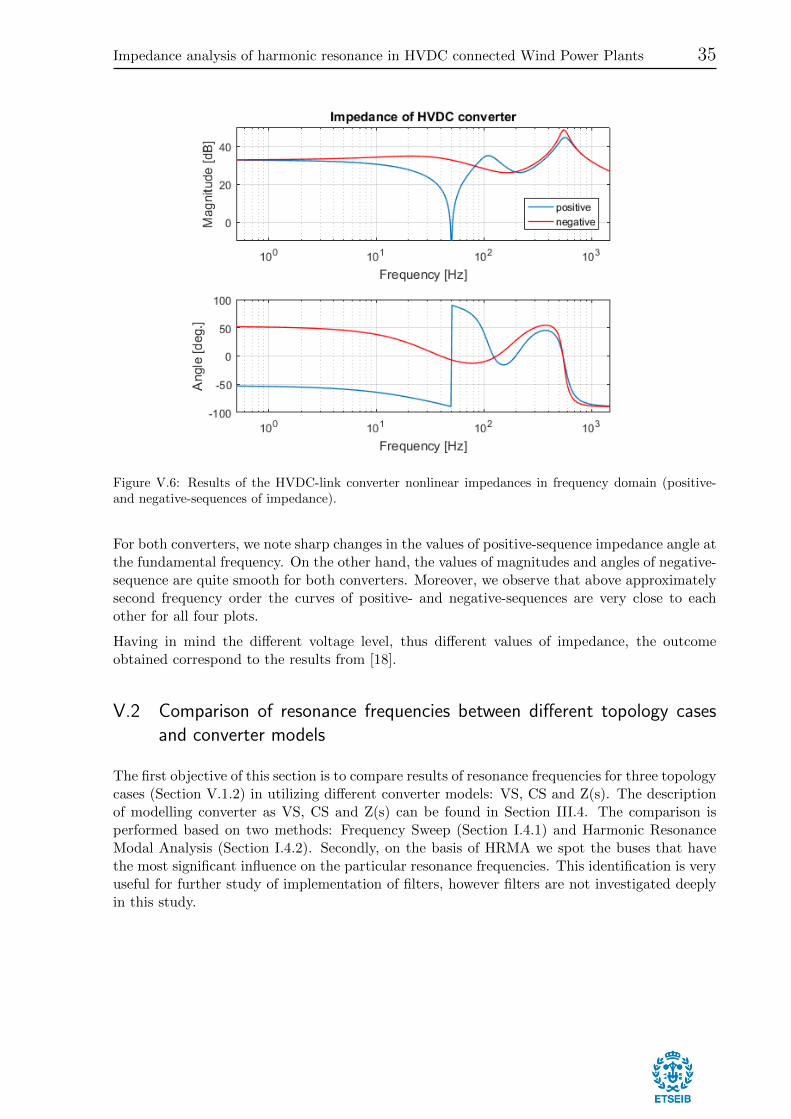
Figure V.6: Results of the HVDC-link converter nonlinear impedances in frequency domain (positive-and negative-sequences of impedance).
For both converters, we note sharp changes in the values of positive-sequence impedance angle atthe fundamental frequency. On the other hand, the values of magnitudes and angles of negative-sequence are quite smooth for both converters. Moreover, we observe that above approximatelysecond frequency order the curves of positive- and negative-sequences are very close to eachother for all four plots.
Having in mind the different voltage level, thus different values of impedance, the outcomeobtained correspond to the results from [18].
V.2 Comparison of resonance frequencies between different topology casesand converter models
The first objective of this section is to compare results of resonance frequencies for three topologycases (Section V.1.2) in utilizing different converter models: VS, CS and Z(s). The descriptionof modelling converter as VS, CS and Z(s) can be found in Section III.4. The comparison isperformed based on two methods: Frequency Sweep (Section I.4.1) and Harmonic ResonanceModal Analysis (Section I.4.2). Secondly, on the basis of HRMA we spot the buses that havethe most significant influence on the particular resonance frequencies. This identification is veryuseful for further study of implementation of filters, however filters are not investigated deeplyin this study.
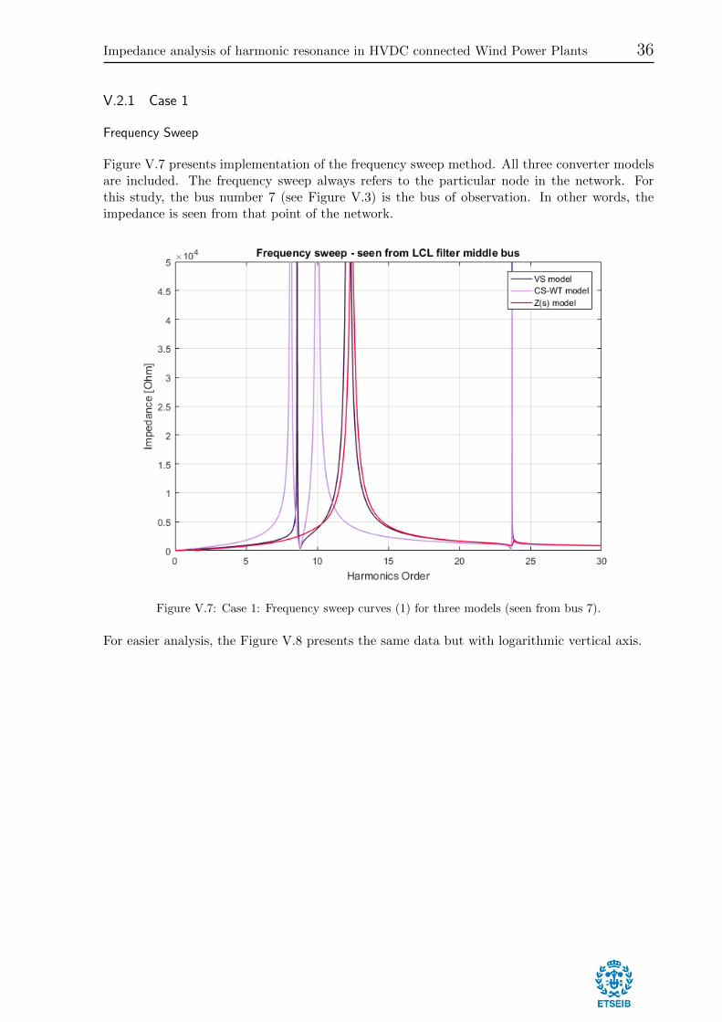
Impedance analysis of harmonic resonance in HVDC connected Wind Power Plants 36
V.2.1 Case 1
Frequency Sweep
Figure V.7 presents implementation of the frequency sweep method. All three converter modelsare included. The frequency sweep always refers to the particular node in the network. Forthis study, the bus number 7 (see Figure V.3) is the bus of observation. In other words, theimpedance is seen from that point of the network.
Figure V.7: Case 1: Frequency sweep curves (1) for three models (seen from bus 7).
For easier analysis, the Figure V.8 presents the same data but with logarithmic vertical axis.

Impedance analysis of harmonic resonance in HVDC connected Wind Power Plants 37
Figure V.8: Case 1: Frequency sweep curves (2) for three models (seen from bus 7).
We can clearly see that the resonance frequencies alter for different models of converters. Ta-ble V.4 presents resonance frequencies values obtained from this analysis. The values of fre-quencies are identified in the points where the impedance curves reach local extreme values.
Table V.4: Case 1: Frequency sweep numerical results of resonant frequencies and corresponding peakimpedance values for three models.
First of all, discover some peaking values of impedance for very low frequency orders (aroundfundamental frequency) in Z(s) model. These peaks are at much lower impedance level than theother values for higher orders. We exclude these peaks from our further analysis, reasoning thatsuch a phenomenon needs more detailed research focused mainly on that problem and it won’tbe an issue in this study.
For VS model (within the examined frequency range) we observe three resonance frequencies.Similarly, in case of CS model there are three resonance frequencies. For the Z(s) model ofconverters only two resonance frequencies are noted (as aforementioned, the low peaks aroundfundamental frequency are ignored).
Moreover, the values of impedance for Z(s) model are significantly reduced comparing to the
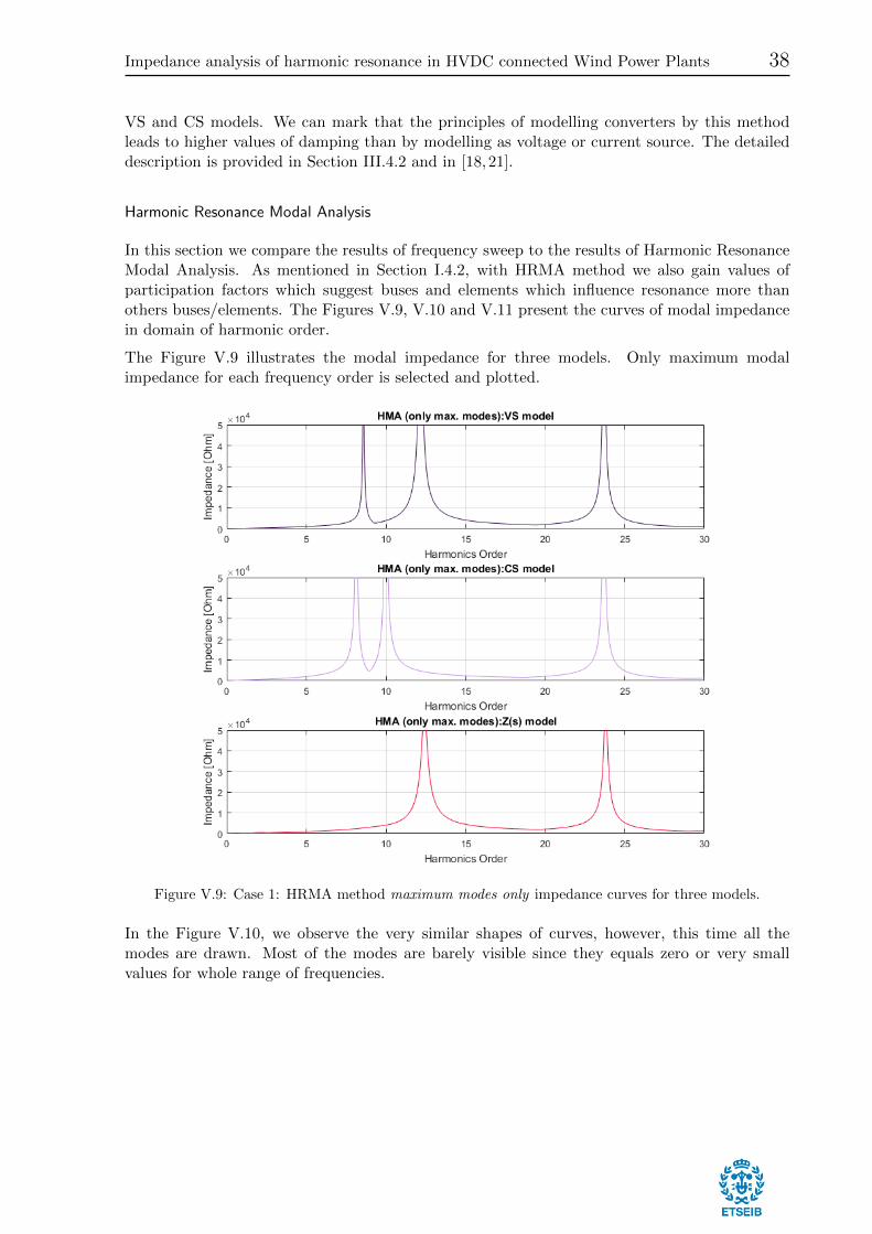
Impedance analysis of harmonic resonance in HVDC connected Wind Power Plants 38
VS and CS models. We can mark that the principles of modelling converters by this methodleads to higher values of damping than by modelling as voltage or current source. The detaileddescription is provided in Section III.4.2 and in [18,21].
Harmonic Resonance Modal Analysis
In this section we compare the results of frequency sweep to the results of Harmonic ResonanceModal Analysis. As mentioned in Section I.4.2, with HRMA method we also gain values ofparticipation factors which suggest buses and elements which influence resonance more thanothers buses/elements. The Figures V.9, V.10 and V.11 present the curves of modal impedancein domain of harmonic order.
The Figure V.9 illustrates the modal impedance for three models. Only maximum modalimpedance for each frequency order is selected and plotted.
Figure V.9: Case 1: HRMA method maximum modes only impedance curves for three models.
In the Figure V.10, we observe the very similar shapes of curves, however, this time all themodes are drawn. Most of the modes are barely visible since they equals zero or very smallvalues for whole range of frequencies.

Impedance analysis of harmonic resonance in HVDC connected Wind Power Plants 39
Figure V.10: Case 1: HRMA method all modes impedance curves for three models.
The graphs above distinguish two modes which are peaking for all thre models - mode 6. and 7.Modal impedance for these modes reaches much higher value at the frequencies of resonance. Themodes that determine the resonances are called critical modes. The critical modes impedancesonly, with full range of impedance, are plotted in the Figure V.11.

Impedance analysis of harmonic resonance in HVDC connected Wind Power Plants 40
Figure V.11: Case 1: HRMA method critical modes impedance curves for three models.
As explained in Section I.4.2, even though the total number of modes equals the number of busesin the network, these modes do not correspond to the network buses exactly. Their correlationis reported by the participation factors presented in Table V.6. Before, Table V.5 presents thecritical modal impedance values and the harmonic orders for frequencies when the critical modalimpedances occur.

Impedance analysis of harmonic resonance in HVDC connected Wind Power Plants 41
Table V.5: Case 1: HRMA numerical results of resonant frequencies and corresponding peak impedancesfor three models.
Table V.6: Case 1: HRMA numerical results of resonant frequencies and participation factors for threemodels.
The study of participation factors is very relevant for localization of the best nodes in a networkfor filter implementation. The participation factors express the significance of a bus in resonanceemission. Therefore, the modification of capacitance/inductance at the point of the network withthe highest participation factor should trigger to the most powerful change of the resonancefrequency. The details about participation factors in Section I.4.2 and [13].
In the study of Case 1, from the values of participation factors, one can easily recognize thatthe buses number 5 and 7 are the two buses which contribute to the resonance frequencies morethan the others. As we can see, these two buses play the lead role in all three different modelswhat indirectly confirms the consistency of three approaches. We also observe only two resonantfrequencies for Z(s) model. From the values of the participation factors, we also derive someconclusions. Since the two resonance frequencies from the first two models are mostly correlatedto the bus 7 and similarly for the one of the resonance frequencies from the Z(s) model, thetwo resonance frequencies from VS and CS models could have been merged into one resonancefrequency from Z(s) model. Otherwise, due to the higher resistance of the Z(s) model, one ofthe resonance frequency could have been smoothed down to the insignificant value.

Impedance analysis of harmonic resonance in HVDC connected Wind Power Plants 42
DIgSILENT Power Factory model
In this simulation, we use the Power Factory model presented in the Figure V.12. The model iscombined of basic RLC elements.
Figure V.12: Case 1: DIgSILENT Power Factory model.
Only two models: VS and CS-WT are simulated. We perform so-called Impedance FrequencyCharacteristic calculation in the software. Figures V.13 and V.14 show the results of frequencysweep for VS and CS-WT model, respectively.
Figure V.13: Case 1: Power Factory impedance curves for VS model (seen from bus 7).

Impedance analysis of harmonic resonance in HVDC connected Wind Power Plants 43
Figure V.14: Case 1: Power Factory impedance curves for CS-WT model (seen from bus 7).
We can examine the figures obtained from the Power Factory software and conclude that, regard-ing resonant frequency values, they are definitely coincident with the ones received from detailanalysis in MATLAB. However, the peak values of impedances are different. The differencesprobably source in the settings of Impedance Calculation for frequency sweep analysis. The stepsize of the simulation was set to the value of 0.1 Hz; furthermore the Automatic Step Size Adap-tation was selected. Hence, difference in the values of impedance occurs. The dependence of thepeak values from the value of step size was checked through similar simulation with differentstep sizes. The observation confirms that the step size influences peak impedance values.
What is more important in this study are the values of the resonance frequencies. The valuesobtained by Power Factory confirms the values gained from MATLAB analysis of both frequencysweep and modal analysis.
Table V.7: Case 1: Power Factory resonant frequencies values for two models.
As aforementioned, the observation of network impedance (frequency sweep) is performed fromthe specified bus in the network (bus 7). Due to the Power Factory software, we can performedthe observation of impedance from each of the bus in the considered case. The results offrequency sweep seen from all 7 buses is presented in the Figure V.15 and V.16, for VS modeland CS model, respectively.

Impedance analysis of harmonic resonance in HVDC connected Wind Power Plants 44
Figure V.15: Case 1: Power Factory impedance curves for VS model (seen from buses 1-7).
Figure V.16: Case 1: Power Factory impedance curves for CS-WT model (seen from buses 1-7).

Impedance analysis of harmonic resonance in HVDC connected Wind Power Plants 45
The examination of the curves above demonstrates that the peaking impedances for both modelsoccur at the same frequencies, regardless the bus of observation. On the other hand, the dips ofimpedance undoubtedly depend on the bus where the observation is performed from. Couplingwith the principles of parallel and series resonance, we can draw the two conclusions. Firstly, theseries resonance frequency depends on the bus in the network i.e. series resonance frequency isdifferent at the different points in the network. Secondly, since the peaks of the impedance, so theparallel resonance frequencies, are the same regardless the bus of observation, we conclude thatthe parallel resonance frequencies do not depend on the point of observation. The confirmationof the latter statement we recognize in the HRMA method. As described in Section I.4.2,the method is utilized in order to investigate the parallel resonance and is not performed forparticular bus, but for entire network. The frequencies collected from that method are exactlythe frequencies obtained for every different case of observation bus in the frequency sweepmethod.
Results comparison
In the three previous paragraphs the results of frequency sweep analysis, harmonic resonancemodal analysis, both performed in MATLAB were presented. Moreover, these results we couplewith frequency sweep tool in Power Factory software. The values of resonance frequenciesobtained ambiguously confirms the correspondence of these three approaches to each other.The values of parallel resonant frequencies are the same for the considered accuracy.
The difference of the impedance peak values are not considered very deeply in this study. How-ever, as aforementioned, these values very often depends on the step size of the calculation.Moreover, the threshold impedance values above which the impedance level is defined as dan-gerous should be assigned individually for each particular case of a network. Furthermore,the values of modal impedance from HRMA method does not exactly correspond to the realimpedance value and should not be compared directly to the values of impedances obtainedfrom frequency sweep or Power Factory tool.
V.2.2 Case 2
The topology Case 2 was presented in Section V.1.2. In this case, the Wind Power Plant consistsof two branches. There is one aggregated Wind Turbine in each branch. The total power ofconnected Wind Turbines is 200 MW.
Frequency Sweep
In the Figures V.17 and V.18 the results of frequency sweep method are presented with linear andlogarithmic impedance scale, respectively. Again, all three models of converters are included.The impedance of the grid is seen again from the bus number 7 i.e. middle bus of LCL filter inthe first branch. Since the branch 1 is the same the branch 2, we could collect the same curvesfor impedance observed from bus 11.

Impedance analysis of harmonic resonance in HVDC connected Wind Power Plants 46
Figure V.17: Case 2: Frequency sweep curves (1) for three models (seen from bus 7).
Figure V.18: Case 2: Frequency sweep curves (2) for three models (seen from bus 7).

Impedance analysis of harmonic resonance in HVDC connected Wind Power Plants 47
Table V.8 presents resonance frequencies values from the graphs above. The values of frequenciesare identified when impedance reaches local extreme values (parallel resonance). This time again,the results of resonance frequencies around fundamental value are ignored.
Table V.8: Case 2: Frequency sweep numerical results of resonant frequencies and corresponding peakimpedance values for three models.
We can note that undoubtedly this time there are four resonant frequencies for Current Sourcemodel. The curve of VS model consists surely of three peaks, however, looking at the values, thefourth one is very close to the other around 12th order. Therefore, it is harder to notice it fromthe graph. The Z(s) model comprises two impedance rises, excluding ones around fundamentalfrequency. The value of impedance of Z(s) model is significantly lower than in other models,similarly to the Case 1. We carry on further conclusions and contemplations about the resonantfrequencies after presenting HRMA results for this case.
Harmonic Resonance Modal Analysis
The Figures V.19-V.21 illustrate the HRMA result curves. Similarly to the previous topologycase, the following graphs shows the curves of maximum modal impedances for each harmonicorder, than modal impedances with respect to the each mode separately and finally, criticalmodes only i.e. the modes that are assigned to the modal impedance peaks.

Impedance analysis of harmonic resonance in HVDC connected Wind Power Plants 48
Figure V.19: Case 2: HRMA method maximum modes only impedance curves for three models.
Figure V.20: Case 2: HRMA method all modes impedance curves for three models.

Impedance analysis of harmonic resonance in HVDC connected Wind Power Plants 49
Figure V.21: Case 2: HRMA method critical modes impedance curves for three models.
Again, the participation factors point out the connotation of each mode to the real buses in thenetwork. Table V.10 presents the participation factors for the detected resonant frequencies i.e.frequencies at which the modal impedance rises occur. The values of critical impedances andcritical modes for each of them are gathered in Table V.9.

Impedance analysis of harmonic resonance in HVDC connected Wind Power Plants 50
Table V.9: Case 2: HRMA numerical results of resonant frequencies and corresponding peak impedancesfor three models.
Table V.10: Case 2: HRMA numerical results of resonant frequencies and participation factors for threemodels.

Impedance analysis of harmonic resonance in HVDC connected Wind Power Plants 51
This time we observe one significant difference between the frequency sweep curves and HRMAcurves. For Z(s) model, one of the frequency that is missing in the frequency sweep methodappears in the HRMA curves. To interpret this we look at the value of the modal impedance forthis resonant frequency or at the figures. The value of critical impedance of critical module ismuch smaller than the other modal critical impedances (for other resonant frequencies). Sincethe resonant frequencies are recognized as the extreme points of impedance curves, peak valueare identified in this way. However, in order to exclude this frequency from the results, furtherinvestigation of for example minimum dangerous impedance would be necessary.
Besides this difference, the results of frequencies converge completely.
From the values of participation factors we derive couple of conclusions. First of all, the values ofparticipation factors for buses of branch 1 (4-7) correspond to the buses of branch 2 (8-11) withthe same values. It shows that from the modal analysis point of view the wind turbine branchesare the same and the participation factor is distributed symmetrically to the two analogousbuses of both branches. Secondly, comparing the results of participation factors for Case 1 andCase 2 we can observe some similarities in apparition of the new resonant frequency. For bothVS and CS-WT model, the lowest resonant frequency stays approximately at the same level, tobe more precise is slightly shifted down to the lower value. The value of participation factor isdivided equally into two analogous buses. The second frequency from Case 1 seems to appear inCase 2 as two resonant frequencies, one greater and the other less than the frequency from Case1. The values of participation factors for both cases for these frequencies appear to confirm thisassumption since their values are again distributed equally and the values are very similar forthe new two frequencies.
On the contrary, in the Z(s) model, the two frequencies stay at approximately the same leveland the new resonance frequency appears independently after adding new branch. As statedbefore, the value of critical impedance is very low.
From the curves of modal impedances with regards to each single node (Figure V.20), we observethat for resonance around 12th order, the values of two modes are at the similar level of modalimpedance for this value of resonance mode 7 and mode 11. This condition disturbs theassumption settled in Section I.4.2 and [13] that only one within the modal impedances is muchgreater than the others.
DIgSILENT Power Factory model
Furthermore, the results of FS and HRMA are compared with the curves acquired from PowerFactory software. Figure V.22 presents the diagram of the network used for calculation.
Figure V.22: Case 2: DIgSILENT Power Factory model.

Impedance analysis of harmonic resonance in HVDC connected Wind Power Plants 52
Again, the models of VS and CS-WT are simulated for Impedance Frequency Characteristiccalculations. Figures V.23 and V.24 present the results of frequency sweep for VS and CS-WTmodels, seen from the middle LCL filter bus i.e. the same bus as for MATLAB model bus 7.
Figure V.23: Case 2: Power Factory impedance curves for VS model (seen from bus 7).

Impedance analysis of harmonic resonance in HVDC connected Wind Power Plants 53
Figure V.24: Case 1: Power Factory impedance curves for CS-WT model (seen from bus 7).
The resonant frequencies for peak impedances are measured by the software tool and presentedin the Table V.11.
Table V.11: Case 2: Power Factory resonant frequencies values for two models.
The values of resonant frequencies are consistent with the values obtained both in FS andHRMA in MATLAB. Again, we present the impedance curves seen from other buses. The buseswhere the impedance is observed are buses 1-7. Since the two branches with wind turbines arethe same, we know that the impedance curves seen from buses 4-7 are the same as seen fromrespective buses 8-11. Therefore the impedance curves for only one branch are sufficient. TheFigure V.25 shows the curves for buses 1-7 for the VS model, while the Figure V.26 illustratethe same curves but for model CS-WT.

Impedance analysis of harmonic resonance in HVDC connected Wind Power Plants 54
Figure V.25: Case 2: Power Factory impedance curves for VS model (seen from buses 1-7).
Figure V.26: Case 2: Power Factory impedance curves for CS-WT model (seen from buses 1-7).

Impedance analysis of harmonic resonance in HVDC connected Wind Power Plants 55
The shapes of the curves indicate the same conclusions like for Case 1 i.e. the series and parallelresonance does depend on and does not depend on the point in the network, respectively. Theprevious section presenting results of Case 1 describes these principles in details.
Results comparison
Similarly to the first case, the results of FS, HRMA and from Power Factory are very similar.For the considered accuracy, the values of corresponding frequencies are exactly the same. Theimportant fact to highlight is that we obtain one resonance frequency more for HRMA comparingto FS in the Z(s) model. Even though the value of modal impedance is quite low comparing tothe other resonance points, the level of impedance dangerous for the network is not identified andcould apparently be already dangerous for the network. The situation suggests the conclusionthat we should always consider both methods together and compare their outputs. Since theamount of data necessary for both methods is very similar, this does not pose a problem duringanalysis.
V.2.3 Case 3
The last topology case is described in Section V.1.2. All installed power (400 MW) and allelements of Wind Power Plant are considered.
Frequency Sweep
Figures V.27 and V.28 present the frequency sweep curves for linear and logarithmic scales,respectively. All three models are included. The bus of observation is again bus 7. All fourwind turbine branches are equal therefore the features of those branches are symmetrical to eachother. The groups of equal bus numbers at the wind turbine branches are: (4, 8, 13, 17), (5,9, 14, 18), (6, 10, 15, 19), (7, 11, 16, 20). Moreover bus 3 and bus 12 are also symmetrical,installed at the end of two symmetrical cables connecting pairs of wind turbine branches.

Impedance analysis of harmonic resonance in HVDC connected Wind Power Plants 56
Figure V.27: Case 3: Frequency sweep curves (1) for three models (seen from bus 7).
Figure V.28: Case 3: Frequency sweep curves (2) for three models (seen from bus 7).

Impedance analysis of harmonic resonance in HVDC connected Wind Power Plants 57
Table V.12 presents resonance frequency values and the peak values of corresponding impedances.The values around the fundamental frequency for Z(s) model are ignored.
Table V.12: Case 3: Frequency sweep numerical results of resonant frequencies and corresponding peakimpedances for three models.
We can observe one additional resonance frequency for each of the VS and CS-WT modelscomparing to Case 2. However, pair of frequencies for each model have very similar valuestherefore, from the figure, could be considered as the one resonant frequency. Further examina-tion and comparison of the frequency sweep results for all considered topology cases is presentedin Section V.2.4.
Harmonic Resonance Modal Analysis
Following Figures V.29, V.30 and V.31 shows the HRMA results. Again, the graphs presentmaximum modal impedances, modal impedances curves for all modes separately and criticalmodes curves alone.

Impedance analysis of harmonic resonance in HVDC connected Wind Power Plants 58
Figure V.29: Case 3: HRMA method maximum modes only impedance curves for three models.
Figure V.30: Case 3: HRMA method all modes impedance curves for three models.
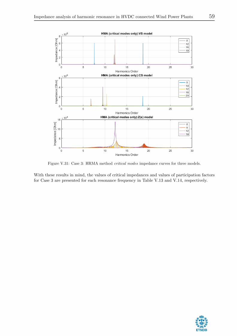
Impedance analysis of harmonic resonance in HVDC connected Wind Power Plants 59
Figure V.31: Case 3: HRMA method critical modes impedance curves for three models.
With these results in mind, the values of critical impedances and values of participation factorsfor Case 3 are presented for each resonance frequency in Table V.13 and V.14, respectively.

Impedance analysis of harmonic resonance in HVDC connected Wind Power Plants 60
Table V.13: Case 3: HRMA numerical results of resonant frequencies and corresponding peak impedancesfor three models.

Impedance analysis of harmonic resonance in HVDC connected Wind Power Plants 61
Table V.14: Case 3: HRMA numerical results of resonant frequencies and participation factors for threemodels.

Impedance analysis of harmonic resonance in HVDC connected Wind Power Plants 62
Similarly to the Case 2, for Z(s) model we obtain one more resonance frequency from HRMAcomparing to frequency sweep. Besides this frequency, the values of equivalent ones are thesame or very similar. Again, the modal impedance value of critical mode for new frequency isvery low.
Finally, we note that the participation factors are not completely symmetrical in some cases. Thesymmetry remains between the pair of branches 1 and 2 or 3 and 4 (the pairs connected to thesame three-winding transformer) but symmetry of participation factors between pair branchesconnected to different three-winding transformers fades away for some cases.
DIgSILENT Power Factory model
Analogously, we compare the results of FS and HRMA with the curves from Power Factorymodel. The model used in this case is presented in the Figure V.32.
Figure V.32: Case 3: DIgSILENT Power Factory model.
The models of VS and CS-WT are simulated for Impedance Frequency Characteristic calcula-tions. Figures V.33 and Figures V.34 present the results of frequency sweep for VS and CS-WTmodel, seen from the middle LCL filter bus i.e. the same bus as for MATLAB model bus 7.

Impedance analysis of harmonic resonance in HVDC connected Wind Power Plants 63
Figure V.33: Case 3: Power Factory impedance curves for VS model (seen from bus 7).
Figure V.34: Case 3: Power Factory impedance curves for CS-WT model (seen from bus 7).

Impedance analysis of harmonic resonance in HVDC connected Wind Power Plants 64
The resonant frequencies for peak impedances are measured in the software tool and presentedin the Table V.15.
Table V.15: Case 3: Power Factory resonant frequencies values for two models.
One more time, the values obtained from Power Factory converge with those we collected fromfrequency sweep analysis in MATLAB. Similarly to the Case 2 analysis, the Figures V.35 andV.36 show the curves for buses 1-7 for the VS model and CS-WT model, respectively.
Figure V.35: Case 3: Power Factory impedance curves for VS model (seen from buses 1-7).

Impedance analysis of harmonic resonance in HVDC connected Wind Power Plants 65
Figure V.36: Case 3: Power Factory impedance curves for CS-WT model (seen from buses 1-7).
The shapes of the curves indicate the similar conclusions like for Case 1 and Case 2.
Results comparison
Similarly to the first and second topology case, the values of received frequencies from all threeapproaches are very similar. Once again, we obtain one more resonant frequency from HRMAcomparing to frequency sweep. Also, we observe similar behaviour of resonances with regard tothe bus of observation.
V.2.4 Comparison between models
In this section we compare the results obtained in three previous sections jointly. The followingfigures and tables demonstrate the behaviour of frequency sweep curves for VS model, CS-WTmodel and Z(s) model. Each model is considered separately but for all three topology cases. Intables the results of resonance frequencies for all topology cases are gathered. The aim of thissection is to identify patterns and any similarities between the topology cases within the threemodels.
V.2.4.1 VS model
Frequency sweep
The following figure presents the frequency sweep curves for all three topology cases. We had atry to group the frequencies in the three groups like indicated in the figure.

Impedance analysis of harmonic resonance in HVDC connected Wind Power Plants 66
Figure V.37: Frequency sweep curves for VS model in three topology cases (seen from bus 7).
Table V.16: Frequency sweep numerical results of resonant frequencies and corresponding peakimpedances for VS model in three topology cases.
We observe clearly that in each next case, the frequencies of first and third group are shifteddownward. This shifting occurs due to the increasing amount of capacitive power in the network.In Case 2, 33kV cable with significant amount of capacitance is connected to the grid. In Case 3,three additional cables are connected i.e. one 150kV and two 33kV collection cables. Thus, wecan mark more significant shift between Case 2 and Case 3 than between first two. The secondgroup (around 12th harmonic order) is becoming more numerous for the cases with multiplebranches, whereas the values stay at the similar level.

Impedance analysis of harmonic resonance in HVDC connected Wind Power Plants 67
Harmonic Resonance Modal Analysis
Figure V.38: HRMA method maximum modes impedance curves for VS model in three topology cases.
Since the frequencies calculated in HRMA are the same to those obtained from frequency sweep,we do not draw more observations. However, we also have at our disposal the values of par-ticipation factors indicating the excitability and observability of the buses in the network. Thevalues of PFs for three topology cases for VS mode are gathered in the Table V.17.

Impedance analysis of harmonic resonance in HVDC connected Wind Power Plants 68
Table V.17: HRMA numerical results of resonant frequencies and participation factors for VS model inthree topology cases.
From the values of PFs we can see the pattern that confirms our assumption created withrespect to resonant frequencies from frequency sweep only. The first group of harmonics seemsto mark the bus 7 (and symmetrical buses within other branches) as the source of this group ofresonances. It touches all topology cases. We have to notice that the values of the PFs could bealso considered as spread quite evenly between the buses. In case of the second group of resonantfrequency (around 12th harmonic order), the bus that is surely indicated by the PFs is the bus7 (and symmetrical ones). Moreover, the more symmetrical branches in the network, the morenumerous the number of resonant frequencies in this group. Further connection of analogousbranches apparently gives more resonant frequencies around 12th frequency order. For the thirdgroup of resonances, we identify two buses (bus 4 and bus 5) indicated by PFs as the two busesparticipating the most in the excitation of the resonance. Bus 4 and bus 5 are the terminals of33 kV collection cable. The observations described above are encapsulated in the Table V.18.

Impedance analysis of harmonic resonance in HVDC connected Wind Power Plants 69
Table V.18: HRMA numerical results of resonant frequencies for VS model in three topology cases withthe dominant bus(es) assigned.
V.2.4.2 CS-WT model
Frequency sweep
Figure V.39: Frequency sweep curves for CS-WT model in three topology cases (seen from bus 7).
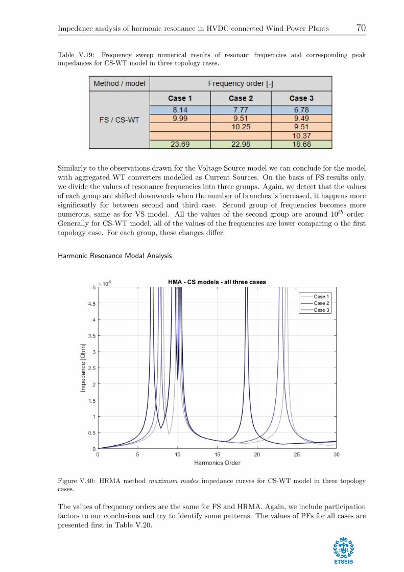
Impedance analysis of harmonic resonance in HVDC connected Wind Power Plants 70
Table V.19: Frequency sweep numerical results of resonant frequencies and corresponding peakimpedances for CS-WT model in three topology cases.
Similarly to the observations drawn for the Voltage Source model we can conclude for the modelwith aggregated WT converters modelled as Current Sources. On the basis of FS results only,we divide the values of resonance frequencies into three groups. Again, we detect that the valuesof each group are shifted downwards when the number of branches is increased, it happens moresignificantly for between second and third case. Second group of frequencies becomes morenumerous, same as for VS model. All the values of the second group are around 10th order.Generally for CS-WT model, all of the values of the frequencies are lower comparing o the firsttopology case. For each group, these changes differ.
Harmonic Resonance Modal Analysis
Figure V.40: HRMA method maximum modes impedance curves for CS-WT model in three topologycases.
The values of frequency orders are the same for FS and HRMA. Again, we include participationfactors to our conclusions and try to identify some patterns. The values of PFs for all cases arepresented first in Table V.20.

Impedance analysis of harmonic resonance in HVDC connected Wind Power Plants 71
Table V.20: HRMA numerical results of resonant frequencies and participation factors for CS-WT modelin three topology cases.
On the basis of PF’s, we gather similar conclusions for CS-WT model than for VS model. ThePF’s for the first two groups of harmonic orders indicates bus 7 (and symmetrical buses at otherbranches) as the bus with highest participation to the harmonic excitation. This time, PF’sof first group of the lowest frequencies are not distributed evenly and mark bus 7 as dominantbus, similarly to second group of frequencies. In the same manner as for VS model, the PF’sof harmonic orders of third group mark the buses 4 and 5 as the buses exciting the resonance.These observations are gathered in the Table V.21.

Impedance analysis of harmonic resonance in HVDC connected Wind Power Plants 72
Table V.21: HRMA numerical results of resonant frequencies for CS-WT model in three topology caseswith the dominant bus(es) assigned.
V.2.4.3 Z(s) model
Frequency sweep
Figure V.41 shows the FS curves for all topology cases derived for Z(s) model.
Figure V.41: Frequency sweep curves for Z(s) model in three topology cases (seen from bus 7).

Impedance analysis of harmonic resonance in HVDC connected Wind Power Plants 73
Table V.22: Frequency sweep numerical results of resonant frequencies and corresponding peakimpedances for Z(s) model in three topology cases.
This time, FS method does not detect resonance frequencies analogous to the lowest ordersgroup for VS and CS-WT model, therefore whole that group does not exist in the Table V.22.The number of peaking impedance points around 12th order also does not increase for multiplebranches cases. However, we observe the equivalent resonances for two groups with values veryclose to the VS model. Similarly to both VS and CS-WT models, we mark the downward shiftof frequencies for analogous group of highest frequencies for each next topology case.
Harmonic Resonance Modal Analysis
Figure V.42: HRMA method maximum modes impedance curves for Z(s) model in three topology cases.
As pointed out in Section V.2, for Z(s) model HRMA detects additional resonant frequencycomparing to FS, but at the low level (relatively to the other critical impedances). These newfrequencies corresponds accurately to the first group of frequencies detected in VS and CS-WTmodel.
Again, we include PFs in the analysis and we identify the buses with the highest values of PFs.The Table V.23 presents PFs values for all topology cases.

Impedance analysis of harmonic resonance in HVDC connected Wind Power Plants 74
Table V.23: HRMA numerical results of resonant frequencies and participation factors for Z(s) model inthree topology cases.
With respect to PF’s, we notice the very similar observation to the models VS and CS-WT.The PF’s of the first and second group of frequencies indicate bus 7 as the one participating themost in the resonances. For the highest order group, similarly, the buses 4 and 5 are identified.These observations are concluded in Table V.24.
Table V.24: HRMA numerical results of resonant frequencies for Z(s) model in three topology cases withthe dominant bus(es) assigned.
V.3 Stability study with respect to topology cases
This section presents the results of stability analysis for the three different already describedtopology cases. The principles of stability analysis are described in Section II.2.2 in the theoret-ical part of the thesis. Only the last model of the network is used i.e. the model containing thenonlinear impedances of the converters Z(s) model - described in Section III.4.2. This modelis considered as the more accurate than two others (VS and CS-WT) presented in the thesis.In short, the stability is evaluated on the basis of phase margin plotted in the Bode diagrams

Impedance analysis of harmonic resonance in HVDC connected Wind Power Plants 75
(Section II.2.3). This stability analysis method for WPP AC grid is considered as still underdevelopment [6]. The sections below present the results separately for each topology case, alsocomparing the values obtained to the previous results from FS and HRMA methods.
V.3.1 Case 1 stability
The Figure V.43 presents the Bode diagram of the considered model used for stability study. Asdescribed in detail in theoretical part, the network is divided into two limped impedances: thesource and the grid. The point of division is behind the HV transformer, looking from the gridside. The positive and negative sequences of source and grid segments are plotted in domain offrequency in the Bode diagrams.
Figure V.43: Case 1: Bode diagram of frequency dependent positive- and negatice-impedances of gridand source.
The points of attention are the crossings of the grid and the source impedances magnitude(zero-dB crossings), regardless the positive or negative sequence. All of them are investigatedwith respect to phase difference of respective curves and the phase margin is calculated. In theFigure V.43 the intersections are marked with purple circles. Figure V.44 presents the sourceand grid curves zoomed in the area of high density of intersections.

Impedance analysis of harmonic resonance in HVDC connected Wind Power Plants 76
Figure V.44: Case 1: Bode diagram (zoomed) of frequency dependent positive- and negatice-impedancesof grid and source.
For each intersection, the stability is assessed by the values of phase margins calculated inMATLAB as described in Section II.2.3. Table V.25 presents the values of frequency orders forwhich the crossings occur and the values of phase margins.

Impedance analysis of harmonic resonance in HVDC connected Wind Power Plants 77
Table V.25: Case 1: Resonance frequencies and the phase margins assigned.
First of all, we observe three points of intersections for each pair of sequence impedances ofsource and grid. Looking at the values of frequencies we obtain very similar values to the FSand HRMA results. Additionally to the frequency values, we obtain the stability assessmenton the basis of phase margins at each intersection (Table V.25). We can see that the groupof highest resonance frequencies could be marked as unstable due to very low values of phasemargin which is very low. Thus, we conclude that unstable operation of this grid can occur ifwaveforms of frequency order around 23.81th order appear in the network. For other resonantfrequencies the stability margin is higher, therefore resonance at those frequencies is less exposedto unstable operation.
V.3.2 Case 2 stability
Similarly to the Case 1, the Bode diagram of the system is provided for Case 2 (Figure V.45and Figure V.46). Regarding the additional branches connected in this topology case, the pointof division for the stability study model is the same i.e. behind HV transformer.

Impedance analysis of harmonic resonance in HVDC connected Wind Power Plants 78
Figure V.45: Case 2: Bode diagram of frequency dependent positive- and negatice-impedances of gridand source.
Figure V.46: Case 2: Bode diagram (zoomed) of frequency dependent positive- and negatice-impedancesof grid and source.

Impedance analysis of harmonic resonance in HVDC connected Wind Power Plants 79
In the Table V.26 the stability assessments by phase margins are gathered for all intersections.
Table V.26: Case 2: Resonance frequencies and the phase margins assigned.
In Case 2, the values of frequencies at the intersections again correspond quite accurately tothe values obtained in the FS and HRMA method. Regarding, the stability assessment baseon the phase margins, we observe again the unstable operation for highest group of resonantfrequencies. Moreover, we mark significant decrease of phase margins for resonances of lowerand medium group of frequency orders.
V.3.3 Case 3 stability
Once again, the system impedance dynamics is plotted on the Bode diagram and the intersectionsof both sequences for grid and source are marked (Figure V.47 and Figure V.48). The point ofdivision is the same as before.

Impedance analysis of harmonic resonance in HVDC connected Wind Power Plants 80
Figure V.47: Case 3: Bode diagram of frequency dependent positive- and negatice-impedances of gridand source.
Figure V.48: Case 3: Bode diagram (zoomed) of frequency dependent positive- and negatice-impedancesof grid and source.

Impedance analysis of harmonic resonance in HVDC connected Wind Power Plants 81
The stability assessments by phase margins are gathered for all intersections in Table V.27.
Table V.27: Case 3: Resonance frequencies and the phase margins assigned.
Once again, the values of frequencies where the intersections between curves occur correspondquite accurately to the values obtained from FS and HRMA methods. The phase marginsof highest frequency is once again very low and marked as possibly unstable, similarly to theprevious cases. The phase margin values of lowest and medium frequency groups are shifteddown even more than in Case 1 and Case 2. While the phase margins of the medium frequencyorder group (around 12th order) is still quite high, the phase margins of the resonance frequenciesaround 9th order (negative grid - positive source and negative grid - negative source) becomeless than the safety margin of 30°assumed in Section II.2.3. The other two intersections aroundthat order (positive grid - positive source and positive grid - negative source) are still above butonly slightly above the safety margin. We conclude that in this case the resonance around 9th
order becomes possibly asymptotically stable (on the boundary of being stable and unstable) oreven unstable.
V.3.4 Comparison to FS and HRMA
From the investigation of Bode diagrams we can compare the results to the ones obtained in bothprevious methods: FS and HRMA. The resonant frequencies are marked at the intersection ofimpedance curves. In this method we analyse both positive and negative impedances of convertermodels, therefore we obtain more resonant frequencies. In previous methods we did not dividethe models into positive and negative sequences. In the following tables (Tables V.28 - V.30),for easy comparison, we can see once again the results of resonant frequency orders obtainedfrom FS and HRMA methods presented in previous sections, as well as, the resonant frequencyorders from Bode diagram analysis.
Table V.28: Comparison of three approaches (I). Frequency sweep.
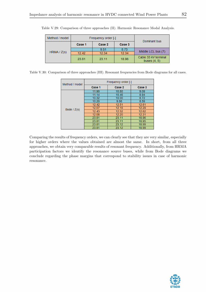
Impedance analysis of harmonic resonance in HVDC connected Wind Power Plants 82
Table V.29: Comparison of three approaches (II). Harmonic Resonance Modal Analysis.
Table V.30: Comparison of three approaches (III). Resonant frequencies from Bode diagrams for all cases.
Comparing the results of frequency orders, we can clearly see that they are very similar, especiallyfor higher orders where the values obtained are almost the same. In short, from all threeapproaches, we obtain very comparable results of resonant frequency. Additionally, from HRMAparticipation factors we identify the resonance source buses, while from Bode diagrams weconclude regarding the phase margins that correspond to stability issues in case of harmonicresonance.

Impedance analysis of harmonic resonance in HVDC connected Wind Power Plants 83
Chapter VI
Approaches to resonance mitigation
To solve harmonic resonance problems the approaches are usually complicated. As described inSection I.3.4, the harmonic resonance depends on several factors and it may vary at differentoperational points or if any change in the network is performed (for example topology changeor installation of new equipment). These facts make the mitigation of the resonance a complexissue. Proper preventive actions during designing phase seems easier to perform and morebeneficial than facing the problem after commissioning through tuning or filtering.
If the network is already built, there are some approaches to limit the problem by additionalassets like passive elements or active filters. In our study, we effectively identified the reso-nance frequencies. Moreover, we determined the main sources of resonances on the basis ofparticipation factors from HRMA method. Thus, to solve the resonance problem, buses markedby participation factors are the candidates where passive or active elements may be installed.Additionally, if converters are present in the network, they may also be utilized, thought theircontrol, to solve or mitigate the resonance problems. This could be especially applicable to theHVDC connected offshore wind farms grids where power converters dominate in the networks.
VI.1 Passive elements
The use of passive elements usually consists of addition of new resistive, inductive or capacitiveelement. Generally, passive elements (filters) are widely applied to limit harmonic propagation,improve power quality, reduce harmonic distortion and provide reactive power compensationsimultaneously. Passive filters are still the first choice when it comes to high voltage or highcurrent grids [7]. Limitations and concerns of passive filters includes [7]:
� They are not adaptable to the changing system conditions (tuned frequency or their sizecannot be changed easily)
� Due to the network impedance in stiff systems very large filters may be required. Thismay bring overcompensation of reactive power or overvoltages on switching
� Power losses can be very significant
� The presence of new passive element (capacitive or inductinve) in a system may causeadditional resonant frequency, therefore careful initial design is crucial
� The ageing, deterioration and temperature effects detune the filter in random manner,therefore the effect is difficult to predict
� Special protective and monitoring devices are required

Impedance analysis of harmonic resonance in HVDC connected Wind Power Plants 84
In our case study of offshore WPP, the most straight-forward method for the resonance mitiga-tion is to add a passive, resistive element to dissipate the energy of oscillations, in other words,to damp the resonance and increase stability margin. Other passive elements: inductance orcapacitance are able shift the resonant frequencies away from the unwanted frequency level.
However, in the real offshore application, addition of new elements brings some problems. Theyrequire additional space in a substation which is apparently located on a offshore platform,therefore the cost of such an implementation is often very high. As aforementioned, new asset,especially resistive, always leads to increased power losses, which have to be effectively dis-sipated or cooled down. On the other hand, both capacitive and inductive elements, besidesshifting of existing resonances, creates new resonance frequency to the offshore network what cancause additional problems. Due to the problems with offshore space for large passive elementsand expected creation of new resonances by new asset, the solution of pure passive elementsimplementation is not recommended in our study case.
VI.2 Active filters, active damping
Generally, active filters can be classified according to the way these are connected in the circuit:series connection, parallel shunt connection and hybrid connections of active and passive filters.For general harmonics reduction, active filtering is usually incorporated with the harmonicproducing equipment itself [7]. The active filters performance for harmonics mitigation is basedon injecting a harmonic current of the same magnitude as that of the nonlinear load into thesystem, but of opposite polarity. Such an active filter is a harmonic current source and could berepresented as a Norton equivalent circuit. The impedance of active filter influences aggregatednetwork impedance, therefore the impedance resonant frequencies can be changed. However, forpurely resonance mitigation, the following approaches of active filtering are proposed from theliterature.
The implementation of hybrid filter (consisting of both passive and active elements) is presentedin the paper [29]. The authors propose the solution for very similar offshore wind farm to theone presented in this study. The best location for placing the filters was chosen on the basis ofpower factors obtained harmonic resonance modal analysis. Moreover, the authors show howhybrid filter contributes positively in reducing the existing harmonics, while the risk of unwantedcurrent magnification due to resonances is limited.
The active method of adding damping resistor is presented in [30]. The principle of the activedamping is to implement damping resistor (in a virtual fashion) by inflicting changes in thecontrolled inductor current. In this way the presence of the resistor is emulated. As the result,virtual damping resistance is introduced to the equivalent control block diagram. It is statedthat this type of active damping control scheme is much easier to be programmed and realized indigital control than conventional damping resistor in series with output capacitor. The authorsalso state that while designing a virtual parallel damping resistor limiting resonance, the issueof stability should be considered, especially in a weak grid. Therefore, consideration of activedamping in this way has to be adopted according to the particular application.
In [31] the authors propose the active damping method for similar impedance model of HVDCconverter to the one used in this study. The active damping [31] is based on injecting a voltagecomponent of counter phase with detected oscillation in order to produce a cancellation effect.The active damping is implemented in the control structure. Three phase voltages are convertedinto d-q components and low pass filter version of measured voltage at PCC is subtracted fromoriginal signal. By that approach, the oscillatory phenomena is effectively damped.

Impedance analysis of harmonic resonance in HVDC connected Wind Power Plants 85
VI.3 Tuning of converter control
As mentioned in the section above, we can influence the performance of a converter by introduc-ing additional control elements i.e. adding additional function of active damping to converters.
Moreover, the tuning of controls which seems to be a very promising approach especially forislanded AC grids, provides other functionality. In principle, through the appropriate adjustmentof control, converter should not be allowed to feed in active power above specified frequency. Thisfrequency limit has to be predefined and should cover all undesired grid resonance frequencies,also regarding other possible operational topologies. This approach simply prevents the converterfrom feeding in active power at the frequencies higher than the limit. Therefore, the gridresonances will not be amplified and harmonic resonance interaction will not occur.
Additionally, the adjustment of converter control combined with the stability analysis approachenables assessment of the system stability. It can be assessed with respect to the changes ofin the converter control and thus in converter impedance. From this, one can conclude how totune the converter in order to provide stable system. The tuning has to be done with respectto detailed specifications and control codes which are the intellectual property of manufacturersand usually are not published.

Impedance analysis of harmonic resonance in HVDC connected Wind Power Plants 86
Chapter VII
Conclusions
In the thesis we investigate the problem of resonance in offshore HVDC connected wind powerplants. The analysis is performed on the basis of 400 MW wind park for three topology cases,for three models of converters and by different methods: frequency sweep, harmonic resonancemodal analysis and stability analysis on the Bode plots. The results are also partially validatedin DIgSILENT Power Factory software. We draw the conclusions step by step within the thesis,however in the following paragraphs the key outcome and observations are assembled.
The first conclusions we can draw having the results of frequency sweep method. The curvescomputed in MATLAB are confirmed by the Power Factory simulation results. The values offrequency are the same in both approaches. The values of impedance peaks are different, butbecause of the difference in step size, we do not consider it as inconsistency. From the results ofFS only, we detect shifting of the resonance frequency in different topology cases. The shifting isexpected and its reason is identified as amount of capacitance (capacitive power) in the networkafter new branches, including capacitive elements, are connected.
Secondly, the values of frequency resonance obtained in harmonic resonance modal analysis con-firms the values obtained in frequency sweep method and in Power Factory software. However,for some cases, the HRMA method returns higher number of resonant frequency values than thenumber obtained from FS. Due to this, both methods should be considered jointly. Moreover,by decomposition of the resonances into different modes, we identify the critical modes respon-sible for each of resonance (in modal domain). Finally, the output of the method includes alsoparticipation factors.
On the basis of participation factors values, first of all, we can extend our conclusions regardingboth methods. The values of participation factors indicate the buses which contribute morethan others to excitement of particular resonance frequency. We identify those buses in eachtopology case for each model. In this way, we observe clear pattern with participation factorsof new resonance frequencies which appear after connecting more branches to the model. Forboth approaches (FS and HRMA), connection of new branches is followed by appearance ofnew resonance frequencies (excluding Z(s) model). The new resonances are very close to oneof existing resonance (emitted from previously connected branches) and have their origin in thenewly connected branches. These observations also clearly tell us about the symmetry in thenetwork.
From the results of frequency sweep analysis performed in Power Factory we can observe thedifference between parallel and series resonance, by combining the impedance curves at thedifferent buses along one branch. We recognize that the series resonance frequencies (marked bydips of impedance curves) depends on the bus which we observe the impedance from, while theparallel resonance frequencies (marked by peaks of impedance curves) are the same, regarding

Impedance analysis of harmonic resonance in HVDC connected Wind Power Plants 87
the bus of observation. These features are confirmed for all topology cases as well as for bothVS and CS-WT models.
Comparing the different converter models, we observe a lot of similarities but also slightlydifferent behaviours for each of them. Generally, we detect lower values of resonance for CS-WT model than for VS model. In Z(s) model the changes in resonant frequencies for differenttopology cases are less significant than for both VS and CS-WT models. In terms of participationfactors analysis, we draw very similar conclusions about the buses participating the most in theresonances. Even though the levels of frequencies are sometimes considerably different, theparticipation factors indicate the same buses as the sources of respective resonance. Hence,the comparison of frequencies between the models gives clear results in terms of emission ofresonances.
The non-linear model of converter impedance Z(s) also provides some interesting outcome. Fistof all, the obtained curves shapes of positive and negative sequences of impedance for bothconverters are consistent with the models found in the literature, often verified by real converters.With Z(s) converter impedances implemented, we obtain similar values of resonant frequencieswhich have the origins in the same buses like in the VS and CS-WT models. From HRMA methodwe collect the similar number of resonant frequencies, while from FS the lowest frequencies arenot detected in this model. Moreover, we observe interesting phenomenon of resonance (peakingimpedance curves) below the fundamental frequency (subsynchronous resonance), which is notthe subject of the thesis. What is more, for different topology cases, the downward shifting ofthe resonant frequencies is very small for the resonances emitted from the WT-converters buses.The other resonance frequencies are not constant and behave similarly as in VS and CS-WTmodels.
The stability analysis were performed to assess the harmonic stability of each topology case. Onthe basis of aggregated model (source and grid) and Nyquist stability criterion interpreted onBode diagram, we identify resonance frequencies and we asses the quality of stability by phasemargin for each identified resonance frequency. The Bode diagram is utilized instead of Nyquistdiagram in order to easily find the intersections and the values of resonant frequencies. First ofall, the frequencies correspond quite accurately to the resonant frequencies obtained from the FSand HRMA methods. This confirms the consistency of all approaches. Due to the considerationof positive and negative sequences we obtain more intersections (more resonance frequencies)than in previous methods, however once again, the values coincide very accurately to the previousmethods. The additional information of phase margins tells us about the quality of stabilityfor each intersection, in other words - the quality of stability for each resonant frequency. Fromthis analysis, we gain information about possible unstable operation of the network in caseof presence of harmonics waveforms at the resonant frequencies (harmonic resonances). Forall three topology cases, group of highest frequency orders are marked unstable while havingnon-sufficient phase margins, thus being exposed to unstable operation hazard in the network.Additionally, for topology cases with more branches, we observe the significant decrease inthe phase margin for the all frequencies above safety margin. This change leads, in topologyCase 3, to the decrease of the phase margin below the safety margin of 30°for lowest group offrequencies. Thus, we conclude that, for our model, highest number of branches (highest numberof aggregated wind turbines) can lead to the problems with stability, which are less probable forlower number of branches.
Application of the methods brings crucial information for further steps of such an analysis likeresonance mitigation. The results obtained are sufficient for further implementation of differentapproaches to mitigate the resonance phenomenon. In this thesis, we discuss and propose someexemplary methods presented in the literature. The active methods of damping and the appro-priate tuning of converters control are considered as relevant in the case of considered offshorewind farm network. Finally, we can highlight very promising, currently developed approach

Impedance analysis of harmonic resonance in HVDC connected Wind Power Plants 88
of resonance mitigation by inverters and rectifiers. Since converters nonlinear impedance canbe influenced by their control, by relevant altering of control we should be able to regulateoutput impedance curves and in this way influence resonances in the system without installingadditional devices.

Impedance analysis of harmonic resonance in HVDC connected Wind Power Plants 89
Chapter VIII
Related environmental impact and costs of thethesis development
VIII.1 Environmental impact of offshore WPP
This section treats about general concerns within environmental impact of offshore wind farms.Since, from environmental point of view, there is almost no difference between AC of DC con-nected wind farms, they are not distinguished. This section gathers some potential impactsof offshore farms, paying attention only to direct environmental impact pathways, excludingpositive aspects of renewable energy production.
The first commercial scale offshore wind farm (Horns Rev 1, installed power of 160 MW) wascommissioned in 2002. Since then, rapid growth of offshore wind energy generation is observed,particularly in northern European waters. As stated in I.2, average capacity of turbines has beenincreasing since then and wind farms are being installed further from the coasts. It is expectedthat the size of offshore wind project will continue increase [32] affecting different environment(further from shores). The relative novelty of the technology makes it difficult to identify all ofthe impacts on environment and effects of those activities.
The most studied impact of offshore wind farms is the impact on marine mammals and seabirds.It is usually of concerns for stakeholders because of legal protection of those spacies [33]. Con-struction of such a wind farm has the greatest impact on marine spacies because of the noise,vessel traffic and pile driving [34]. Those activities could potentially cause hearing damages,spatial displacement to avoid noise or collisions and disturbances from vessels movements [35].During operation of wind farms, underwater sound levels also can reach dangerous levels, dis-turbing acoustic communication of marine mammals [36] and fishes [37].
Of greatest concern is also the impact of seabirds. Mortality can be caused by collision withblades. This may affect birds migrating through the area as well as those that breed or foragein the vicinity [38].
Another issue to look at is the emission of electromagnetic field by submarine cables transmittingthe electricity onshore. This can also affects the movements and navigation of spacies that aresensitive to electromagnetic fields (mainly fishes and sea turtles) [39].
The species of concern will of course differ among regions depending on climate, occurrence ofthose species or regulations and protection statuses.

Impedance analysis of harmonic resonance in HVDC connected Wind Power Plants 90
VIII.2 Temporary planning and costs of thesis development
In this section we present the cost of development of the master thesis. We consider direct andindirect costs of the work. The direct costs are expanses that could be easily connected to thework/product etc. This includes for example items such as software, equipment, labour, rawmaterials. On the other hand, indirect costs go beyond the costs associated with creating aparticular product. For example, the materials and supplies needed for the company’s day-to-day operations (office rental, desktop computers, cell phones). These costs contribute to thecompany as a whole, but they are not assigned to particular work/project.
As the result, in our case, the costs are divided into:
1. Direct costs (cdirect):
� Labour cost (clabour)
� Software cost (csoftware)
2. Indirect costs (crindirect)
� Total indirect costs (office rent, desk, electricity etc.) is assumed to be proportionalto direct costs.
In the calculations the following values are assumed:
� Time frame of work (T ): 20 weeks
� Work week time (tweek): 32.5 h/week
� Pay rate - cost of employment for employer (pemployer): 25 EUR/h
� Cost of software (cPF , cML): 1500 EUR (DigSILENT Power Factory), 2000 EUR (MAT-LAB)
� Indirect costs (office rent, electricity, desk, water) are estimated as 25% of direct costs(rindirect)
� VAT 21% (Spain)
� Additional time for further development: 20 weeks
Hence, the cost of the master thesis development till now is:
Ctotal = cdirect + cindirect
where direct cost is:
cdirect = clabour + csoftware = pemployer · tweek · T + cPF + cML
and indirect cost is:cindirect = rindirect · cdirect
Thus, excluding VAT, the values are:
clabour = 16250 EUR
csoftware = 3500 EUR

Impedance analysis of harmonic resonance in HVDC connected Wind Power Plants 91
cdirect = 19750 EUR
cindirect = 4937.5 EUR
And the total cost, including VAT is:
ctotal = 29871.88 EUR
which gives the average value per hour:
cperHour = 45.96 EUR/h
For the purpose of further development (for example implementation of resonance mitigationmethods), the time frame of next 20 weeks is assumed. The cost of labour is obviously propor-tional to the working time, however due to the fact that the employer will not pay again forthe licences of the software, the value per hour for total project of 40 weeks will decrease to thelevel of 41.88 EUR/h.

Impedance analysis of harmonic resonance in HVDC connected Wind Power Plants 92
Reference
[1] REN21, Renewables 2016 - Global Status Report. Renewable Energy Policy Network for the21st Century. 2016.
[2] WWEA, Qarterly Bulletin. 1 March 2016.
[3] GEWC, Global Wind Report - Annyal Market Update. 2015.
[4] EWEA, The European offshore wind industry - key trends and statistics 2015. February2016.
[5] G. F. Reed, H. A. A. Hassan, M. J. Korytowski, P. T. Lewis, and B. M. Grainger, “Com-parison of hvac and hvdc solutions for offshore wind farms with a procedure for systemeconomic evaluation,” in Energytech, 2013 IEEE, pp. 1–7, May 2013.
[6] C. Buchhagen, C. Rauscher, A. Menze, and J. Jung, “Borwin1-first experiences with har-monic interactions in converter dominated grids,” in International ETG Congress 2015;Die Energiewende-Blueprints for the new energy age; Proceedings of, pp. 1–7, VDE, 2015.
[7] J. Das, Power System Harmonics and Passive Filter Designs. IEEE Press Series on PowerEngineering, Wiley, 2015.
[8] F. De La Rosa, Harmonics and Power Systems. Electric Power Engineering Series, CRCPress, 2006.
[9] J. Arrillaga and N. Watson, Power System Harmonics. Wiley InterScience electronic col-lection, Wiley, 2004.
[10] M. Bradt, B. Badrzadeh, E. Camm, D. Mueller, J. Schoene, T. Siebert, T. Smith, M. Starke,and R. Walling, “Harmonics and resonance issues in wind power plants,” in Transmissionand Distribution Conference and Exposition (T D), 2012 IEEE PES, pp. 1–8, May 2012.
[11] I. A. report prepared by Load Characteristics Task Force., “The effects of power systemharmonics on power system equipment and loads,” IEEE Transactions, 1985.
[12] R. H. Park, “Two-reaction theory of synchronous machines generalized method of analysis-part i,” Transactions of the American Institute of Electrical Engineers, vol. 48, no. 3,pp. 716–727, 1929.
[13] W. Xu, Z. Huang, Y. Cui, and H. Wang, “Harmonic resonance mode analysis,” IEEETransactions on Power Delivery, vol. 20, pp. 1182–1190, April 2005.
[14] G. C. Verghese, I. J. Perez-arriaga, and F. C. Schweppe, “Selective modal analysis withapplications to electric power systems, part ii: The dynamic stability problem,” IEEETransactions on Power Apparatus and Systems, vol. PAS-101, pp. 3126–3134, Sept 1982.

Impedance analysis of harmonic resonance in HVDC connected Wind Power Plants 93
[15] R. Bellman, R. E. Bellman, R. E. Bellman, R. E. Bellman, and E.-U. Mathematicien,Introduction to matrix analysis, vol. 960. SIAM, 1970.
[16] I. J. Perez-Arriaga, G. C. Verghese, and F. C. Schweppe, “Selective modal analysis withapplications to electric power systems, part i: Heuristic introduction,” ieee transactions onpower apparatus and systems, no. 9, pp. 3117–3125, 1982.
[17] L. Pham, “A review of full scale converter for wind turbines,” URL https://www. academia.edu/5759035/A Review of Full Scale Converter for Wind Turbines, p. 8.
[18] H. Liu and J. Sun, “Voltage stability and control of offshore wind farms with ac collectionand hvdc transmission,” IEEE Journal of emerging and selected topics in power electronics,vol. 2, no. 4, pp. 1181–1189, 2014.
[19] J. Sun, “Impedance-based stability criterion for grid-connected inverters,” IEEE Transac-tions on Power Electronics, vol. 26, no. 11, pp. 3075–3078, 2011.
[20] R. D. Middlebrook, “Input filter considerations in design and application of switching reg-ulators,” IAS’76, 1976.
[21] H. Liu and J. Sun, “A study of offshore wind hvdc system stability and control,” in Proceed-ings of 10th International Workshop on Large-Scale Integration of Wind Power into PowerSystems as well as on Transmission Networks for Offshore Wind Power Plans, 2011.
[22] J. Sun, “Small-signal methods for ac distributed power systems–a review,” IEEE Transac-tions on Power Electronics, vol. 24, no. 11, pp. 2545–2554, 2009.
[23] Z. Bing, K. J. Karimi, and J. Sun, “Input impedance modeling and analysis of line-commutated rectifiers,” IEEE Transactions on Power Electronics, vol. 24, no. 10, pp. 2338–2346, 2009.
[24] M. Cespedes and J. Sun, “Impedance modeling and analysis of grid-connected voltage-source converters,” IEEE Transactions on Power Electronics, vol. 29, no. 3, pp. 1254–1261,2014.
[25] E. Larsen, G. Drobnjak, and H. Elahi, “Standardization of vsc-hvdc interface with offshorewind generation,” Proc. 11th Int. Workshop Large-Scale Integr. Wind Power Power Syst.,2012.
[26] IEC, “Series 61000 standards,” from 1990.
[27] CENELEC, “En 50160 - voltage characteristics of electricity supplied by public distributionsystems,” Brussels, 1994.
[28] IEEE, “Recommended practice and requirements for harmonic control in electrical sys-tems,” 1992.
[29] K. N. B. M. Hasan, K. Rauma, A. Luna, J. I. Candela, and P. Rodrıguez, “Harmonic com-pensation analysis in offshore wind power plants using hybrid filters,” IEEE Transactionson Industry Applications, vol. 50, no. 3, pp. 2050–2060, 2014.
[30] X. Chen, C. Y. Gong, H. Z. Wang, and L. Cheng, “Stability analysis of lcl-type grid-connected inverter in weak grid systems,” in Renewable Energy Research and Applications(ICRERA), 2012 International Conference on, pp. 1–6, IEEE, 2012.
[31] M. Amin, M. Molinas, and J. Lyu, “Oscillatory phenomena between wind farms and hvdcsystems: The impact of control,” in 2015 IEEE 16th Workshop on Control and Modelingfor Power Electronics (COMPEL), pp. 1–8, IEEE, 2015.

Impedance analysis of harmonic resonance in HVDC connected Wind Power Plants 94
[32] EWEA, “The european offshore wind industry - key trends and statistics 2013,” tech. rep.,European Wind Energy Association, Brussels, Belgium, 2014.
[33] H. Bailey, K. L. Brookes, and P. M. Thompson, “Assessing environmental impacts of off-shore wind farms: lessons learned and recommendations for the future,” Aquatic biosystems,vol. 10, no. 1, p. 1, 2014.
[34] S. Dolman and M. Simmonds, “Towards best environmental practice for cetacean conser-vation in developing scotland’s marine renewable energy,” Marine Policy, vol. 34, no. 5,pp. 1021–1027, 2010.
[35] P. T. Madsen, M. Wahlberg, J. Tougaard, K. Lucke, and P. L. Tyack, “Wind turbineunderwater noise and marine mammals: implications of current knowledge and data needs,”Marine Ecology Progress Series, 2006.
[36] J. Tougaard, O. D. Henriksen, and L. A. Miller, “Underwater noise from three types ofoffshore wind turbines: Estimation of impact zones for harbor porpoises and harbor seals,”The Journal of the Acoustical Society of America, vol. 125, no. 6, pp. 3766–3773, 2009.
[37] M. Wahlberg and H. Westerberg, “Hearing in fish and their reactions to sounds from offshorewind farms,” Marine Ecology Progress Series, vol. 288, pp. 295–309, 2005.
[38] M. Desholm and J. Kahlert, “Avian collision risk at an offshore wind farm,” Biology letters,vol. 1, no. 3, pp. 296–298, 2005.
[39] T. Tricas and A. B. Gill, “Effects of emfs from undersea power cables on elasmobranchsand other marine species.,” 2011.