CLIMATE RESEARCHClim Res

Vol. 46: 1–14, 2011doi: 10.3354/cr00939

Published online January 20

1. INTRODUCTION

Tourism plays a fundamental role in the Austrianeconomy. In 2005, 21.6 billion Euros in direct and indi-rect value added [8.8% of the gross domestic product(GDP)] resulted from tourism activity. There weremore than 30 million arrivals and 120 million overnightstays (Laimer & Smeral 2006). A large share of tourismactivity takes place in the 345 municipalities with majorski areas. These account for 44 million of the 60 millionovernight stays in the winter season. Owing to theimportance of the ski tourism industry, researchers andthe public have become particularly concerned aboutthe consequences of climate change.

Numerous studies have focused on understandingthe past and possible future changes in winter temper-ature and precipitation patterns on the length of skiseasons and snow reliability, not only in Austria butalso in other countries with a substantial skiing indus-try (Switzerland, France, Italy, USA, Canada, etc.).Several studies have been conducted covering natural

snow conditions (Harrison et al. 1986, Lamothe & Péri-ard Consultants 1988, Galloway 1988, Lipski &McBoyle 1991, McBoyle & Wall 1992, König & Abegg1997, Breiling & Charamza 1999, Elsasser & Bürki2002, Fukushima et al. 2002, Abegg et al. 2007). Morerecently, studies have also begun to examine theimpact of climate change on the future importance ofartificial snowmaking (Scott et al. 2003, 2006, Teichet al. 2007, Hennessy et al. 2008, Scott et al. 2008,Steiger & Mayer 2008). These studies (supply-sidestudies) have thoroughly described changes in climaticconditions and their overwhelmingly negative effectsin ski areas.

However, comparatively little effort has been madeto systematically quantify the relationship betweenpast weather conditions and the economic performanceof ski areas (demand-side studies). In other words,although climate change is recognized as being animportant factor in alpine tourism, the impact of cli-mate variability on tourism demand over recent de-cades has largely been neglected in studies, with 3

© Inter-Research 2011 · www.int-res.com*Email: christoph.toeglhofer@uni-graz.at

Impacts of snow conditions on tourism demand inAustrian ski areas

Christoph Töglhofer1, 2,*, Franz Eigner1, Franz Prettenthaler1, 2

1Wegener Center for Climate and Global Change, University of Graz, Leechgasse 25, 8010 Graz, Austria2Joanneum Research, Centre for Economic and Innovation Research, Elisabethstraße 20/II, 8010 Graz, Austria

ABSTRACT: Major research efforts have been devoted to studying the impacts of climate change onsnow conditions in ski areas, including snow making as a technical adaptation strategy in recentyears. However, little attention has been paid to quantifying past demand changes owing to short-term climate variability. This paper examines the impacts of snow conditions on tourism demand in185 Austrian ski areas in the period 1972/1973 to 2006/2007. For the majority of areas, a positive rela-tionship is found between overnight stays and snow conditions; however, overnight stays in higher-lying areas typically show no dependency on snow conditions. Instead, some of them negativelydepend on average Austrian snow conditions. Overall, a 1 standard deviation change in snow condi-tions led to a change in overnight stays of 0.6 to 1.9%, with estimates from the most reliable paneldata models of 0.6 and 1.1%. Impacts were significantly higher for particular regions and for extremeseasons. However, temporal analysis reveals that impacts have decreased in recent years, probablyowing to the major increase in snowmaking.

KEY WORDS: Climate variability · Tourism · Snow · Regression analysis · Panel data · Austria

Resale or republication not permitted without written consent of the publisher

OPENPEN ACCESSCCESS

Clim Res 46: 1–14, 2011

recent exceptions. Dawson et al. (2009) used an ana-logue approach for examining the impact of anom-alously warm winters on total skier visits and operatingprofits in the northeast region of the US. They com-pared the economic performance of the ski industry inclimatically normal winters and in winters which canbe regarded as representative of future average cli-mate conditions under different greenhouse gas emis-sions scenarios. Hamilton et al. (2007) chose an ARMAXtime series model to examine daily variations in visitornumbers for 2 New England ski areas. They coveredsnow conditions both in the respective areas and in thecity of Boston to check for the influence of urban snowconditions (‘backyard hypothesis’). Similarly, Shih etal. (2009) used multiple linear regression models toanalyze the weather dependency of ski lift ticket salesat 2 Michigan ski resorts. All of these studies found aclear relationship between snow or temperature condi-tions and the economic indicators examined.

Other, lesss specific studies have been conducted ona wider spatial and temporal scale to determine themore general relationship between weather andtourism demand. Agnew & Palutikof (2006) appliedtime series regression models to look into the impactsof temperature, precipitation and sunshine in the UKon the demand for international and domestic tourism.Bigano et al. (2005) used a similar approach for tourismdemand in Italian regions, and expanded the regres-sion models by using panel estimations. Although theresults were relatively weak for the UK, temperaturewas found to correlate positively with Italian tourismdemand in summer, and negatively with tourism de-mand in alpine regions in winter. The authors sug-gested that the latter effect may be due to the negativeinfluence of high temperatures on the skiing season. Aseries of other studies (Maddison 2001, Lise & Tol 2002,Hamilton et al. 2005, Bigano et al. 2006) used cross-sectional data to determine the optimal temperaturefor international tourism, but did not specifically incor-porate the temperature requirements of alpine wintertourism into their models.

The present study goes beyond other demand-sidestudies in that it considers the link between snow con-ditions and tourism demand both on a local scale andfor a relatively large number of cases (185 ski areas).When focusing on weather impacts in alpine regions,working on a local scale is essential, as this makes itpossible to incorporate the complex microclimatic con-ditions across regions. Furthermore, using a largenumber of cases allows for comparison of sensitivitiesbetween different regions. In addition, the utilizationof data for 34 winter seasons means that changes insnow sensitivity over time can be observed and thattime series characteristics of demand data can also betaken into account.

2. DATA AND METHODOLOGY

In this section, we present an approach for determin-ing the sensitivity of tourism demand in Austrian skiareas to seasonal snow conditions. Tourism demand isexpected to depend, among other ‘unknown’ factors,on the meteorological conditions in the ski areas, thesupply of tourism infrastructure and the economic con-ditions prevailing in the guests’ countries of origin. Westart the analysis by discussing the nature of the dataand the expected influence of the variables on localtourism demand. The formal econometric model speci-fications are then presented.

2.1. Data preparation

As a first step, economic and meteorological data werecollected for the major Austrian ski areas. This wasparticularly challenging because statistical tourism dataprovided by Statistics Austria (2008) is given on a munic-ipal level whereas meteorological data are given eitherfor selected measurement stations or on a grid basis.Hence, municipalities with skiing activities werematched to ski areas, and the altitude, size and exactlocation of the ski areas were determined, based onseveral data sources (Joanneum Research 2008,bergfex 2009, BEV 2009). The altitudes and coordinatesof the ski areas were then provided for the meteorolog-ical model and snow indices were calculated. Altogether,345 municipalities were assigned to 202 ski areas; therespective areas met the chosen size constraint of morethan 5 transport facilities or at least 1 cable car in thearea. Because lack of data meant that 17 areas (mostlysmall) had to be excluded, model calculations werecarried out for the remaining 185 ski areas.

2.2. Tourism demand data

In general, data on ski lift ticket sales should be moreresponsive to changes in weather conditions thantourism indicators such as overnight stays or arrivals.These data include sales from day trippers, who are par-ticularly flexible and sensitive to adverse weather condi-tions. By contrast, overnight stays or arrivals might berelatively less responsive, because terms of cancellationmight encourage people to set out on a journey evenwhen the weather forecast is unfavourable. Once thetourists have arrived in ski areas, they have the opportu-nity to replace skiing with some other activity during pe-riods of bad weather conditions, especially in medium tohigh price destinations. The problem is, however, thatconsistent data on ski lift ticket sales are only availablefor a limited number of ski areas. Hence, unlike other re-

2

Töglhofer et al.: Snow conditions and tourism demand

cent studies relying on case study data on ski area visi-tors (Hamilton et al. 2007, Shih et al. 2009), we based ouranalysis on overnight stays in ski areas.

Figs. 1 and 2 show the Austrian municipalities cate-gorized according to the mean altitudes of ski areas andthe development of overnight stays in the winter sea-sons from 1972/1973 to 2006/2007 for the respective al-titude categories. Overall, the number of overnightstays has grown in 27 out of 34 seasons, with the mostnotable exceptions occurring in the mid-1990s. How-ever, looking at the different altitude categories revealsthat, in the last 20 yr, considerable growth can only beobserved in municipalities with ski areas above 1800 mand in non-skiing municipalities. By contrast, decliningtrends predominate in lower-lying municipalities(<1200 m), typically those of a smaller area.

2.3. Meteorological data

Consistent snow measurements for longer timeseries, as needed for our analysis, could only be foundfor a limited number of measurement stations andwould not have covered regional snow variations andrespective altitude of ski areas. Thus, we chose to takedata from a snow cover model, which uses air temper-ature and precipitation data to reconstruct historicsnow conditions for each of the given ski area coordi-nates, both for the lowest and mean altitudes. The datawere provided by the Central Institute for Meteorology

and Geodynamics (ZAMG 2009) and are available on a1 × 1 km grid for the period 1973 to 2006. Of course,although this procedure creates a more consistent dataset, the underlying uncertainties regarding the exten-sive assumptions behind the snow model (e.g. spatialinterpolation of data, assumptions about accumulationand ablation of snow cover) also need to be taken intoaccount. For a more detailed discussion of the model,see Beck et al. (2009).

3

Fig. 1. Austrian municipalities categorized according to the mean altitudes of ski areas

Winter season

Ove

rnig

ht s

tays

(in

mill

ions

)

19731975

19771979

19811983

19851987

19891991

19931995

19971999

20012003

20052007

0

10

20

30

40

50

60

Fig. 2. Development of overnight stays in the winter seasons1972/1973 to 2006/2007 dependent on the mean altitude ofthe ski areas in the respective municipalities. See Fig. 1 leg-end for altitude categories. Data source: Statistics Austria

(2008)

Clim Res 46: 1–14, 2011

Based on the results from the snow cover model, sev-eral snow indices were calculated on a seasonal basisfor the lowest and mean altitude of the ski areas: meansnow depth (Smean, cm), days with snow depth >1 cm(Sday1, d) and days with snow depth >30 cm (Sday30).In addition, for some analyses we considered mean airtemperature (Tmean, °C) as well as the urban snow con-ditions (Sday1,cities) and weighted mean snow condi-tions, with the weights being the overnight stays(Sday1,AVG).

We conducted our analysis using all of these weatherindices but, for the sake of brevity, we focus on theSday1 index to illustrate our results for individual skiareas. We chose this index based on a comparison ofdata for 17 measurement stations, which are locatedclose to the lowest altitudes of ski areas, with the re-spective snow indices from the snow cover model. Thisanalysis revealed a systematic underestimation of snowdepths by the snow cover model. Thus, in reality, theSday1 index portrays higher snow depth than just 1 cm.Furthermore, an evaluation of the model uncertaintyshows smaller deviations from measurement data forSday1 than for Sday30 or Smean; correlations betweenmodel and measurement data were also higher forthis index.

Analyzing the snow indices in more detail, we seethat the climatological mean of all of the snow indices,not surprisingly, increased with altitude. The standard

deviation (SD) varied substantially across ski areas,with higher-lying areas generally exhibiting less datavariability for Sday1 but more variability for Sday30 andSmean. All snow indices exhibited negative trends forthe vast majority of areas, with more pronouncedtrends observed in higher-lying areas. Fig. 3 illustratesthe climatological mean, SD and trend for Sday1 in themean altitudes of ski areas.

Overall, we expect the number of overnight stays tobe positively affected by good snow conditions, withlower-lying areas being particularly dependent. Ifthere is enough snow depth in lower lying areas,tourists will tend to go there. This should be especiallytrue for such ski areas in Tyrol, Salzburg and Vorarl-berg, which are easy to reach from Germany, and forsuch ski areas in Lower and Upper Austria, which arecloser to Vienna compared with competing destina-tions in Salzburg and Tyrol. By contrast, it is alsoexpected that higher-lying areas benefit more fromwinters and preceding winters with bad snow condi-tions, as they are considered to be more snow reliable.

2.4. Other data

For the panel data models, we used several othernon-climatic variables that are likely to have an impacton tourism demand. First, supply of accommodation

4

Mean (d)

<6060 to <90

90 to <120

120 to <150

>150

Standard deviation (d)

<1010 to <15

15 to <20

20 to <25

>25

Negative and statistically significant trend

Fig. 3. Climatological mean, standard deviation and trends for days with snow depth >1 cm for the mean altitude of ski areas in the winter seasons 1972/1973–2005/2006. Data source: ZAMG (2009)

Töglhofer et al.: Snow conditions and tourism demand

was considered by using the number of beds in a skiarea (Statistics Austria 2008). Additional capacity islikely to enhance the number of overnight stays in anarea. Furthermore, the tourism forecasting and demandliterature suggests that a bundle of economic variablesinfluences the level of overnight stays (see Song et al.2009). We thus included income and price variables byusing GDP, consumer price indices (CPI) and exchangerates (OECD 2008). We closely follow Luzzi & Flückiger(2003) by calculating income and price variablesweighted by the guests’ origin in each ski area. Theincome index is expected to influence tourism demandpositively whereas relative price levels are expected toinfluence tourism demand negatively.

2.5. Time series regression models

In order to estimate the impacts of weather conditionsin each of the ski areas, we used an autoregressive dis-tributed lag (ADL) model. In principal, our ski area spe-cific model has the same form as the models used inBigano et al. (2005) and Agnew & Palutikof (2006), ex-cept that we worked on the local rather than on the na-tional or provincial scale. Instead of putting the highlycollinear weather indices into a single model, we usedonly one index at a time and repeated calculations forall indices. Accordingly, in order to explain variations inovernight stays in winter on a seasonal basis t (nightst)our model contains lags of the dependent variable(nightst –1, nightst –2) as well as the respective meteoro-logical variable (snowt) and its lag (snowt–1), and can bewritten for each of the 1, …, n ski areas as:

(1)

where εt represents the error term and β0 to β4 therespective coefficients.

A lag length of 1 was chosen for snowt, whereas thedependent variable enters the equation with 2 lags.Dynamic modelling by including lagged dependentvariables in the regression is recommended in thepresence of temporal autocorrelation in the residualsand/or high persistency in the dependent variable. Theinclusion of a lagged dependent variable then reducesthe amount of potential spurious regression, whichmay lead to wrong inferences and potential inconsis-tent estimation. Apart from that, obtained autoregres-sive coefficients are often of interest by themselves,because they allow both tourist expectations and habitpersistence to be taken into account. These behaviourpatterns are expected to be stable, as people who havebeen on holiday to a particular destination and liked ittend to return to that destination. Uncertainty isreduced and knowledge about the destination spreads

by word of mouth, and this may well play a moreimportant role in destination selection than commer-cial advertising (Song et al. 2009).

We took the logarithm of overnight stays and thesnow index. This is common in the literature fortourism demand data, because transforming to loga-rithms produces time series with approximately con-stant variance over time. Otherwise, it is often the casethat the higher the level of a series rises, the greaterthe variation observed around that level. Taking loga-rithms for the snow index also enables us to interpretcoefficients from the regression models directly aselasticities (log–log specification).

The model for each of the ski areas was tested forresidual autocorrelation (Breusch 1978, Godfrey 1978),functional form (Ramsey 1969), heteroscedasticity(Breusch & Pagan 1979) and the distribution of theresiduals (Jarque & Bera 1980). A model can be consid-ered as statistically acceptable when none of theapplied tests indicate a violation of the underlyingassumptions. All tests were conducted with a signifi-cance level of 5%.

The snow elasticities (β3) for each area give the per-centage change in overnight stays for a 1% increase insnow days. However, it is important to note that adirect comparison of the elasticities of different skiareas is not particularly fruitful because of the variabil-ity in the original snow data. Therefore, the impact of achange in snow conditions in a ski area is given as thepercentage change in overnight stays when the re-spective snow index varies by 1 SD (σ). This gives thefollowing formula:

(2)

Putting it differently, the impact of a 1 SD changemeasures not only the sensitivity of the examineddemand indicator given by the demand elasticity butalso the probability that a certain impact occurs. Theprobability of such a standard deviation change obvi-ously depends on the distribution of the snow index.Under a normal distribution, the probability of a winterwith a >1 SD decrease in the index would be 15.9%.For the Sday1 index, for example, this is approximatelytrue for the median ski area (14.7%), but altogether theestimated probabilities vary with the skewness andkurtosis of the respective indices. As an alternative toSD, we could estimate some other risk measure, e.g.the 5 or 10% quantile, and speaking in the language offinancial risk management, it could be referred to as‘overnight stays at risk’. However, in this case moreattention would need to be placed on the modelling ofthe weather index, as the use of 34 seasonal observa-tions makes it more difficult to estimate quantiles, par-ticularly because here it is the tails of the distributionswhich are of more interest.

impactnightssnow

snowchange snow s= =β σ σ3 log log%%

ΔΔ nnow

log log lognights nights nightst t t= + +− −β β β0 1 1 2 22

3 4 1

++ +−β β εlog logsnow snowt t t

5

Clim Res 46: 1–14, 2011

2.6. Panel data models

In order to estimate the impact of the variables ontourism demand in ski areas, the ADL model type, asused for the time series regressions before, was alsoapplied to the whole data set, making up a panel with185 cross-section units and a time dimension of34 units. As this model gives more degrees of freedom,we additionally used variables for the supply of accom-modation (bedsit), income (gdpit) and prices (ppit),where the subscripts i and t represent the specific skiarea and the season respectively. Therefore, our modelspecification has a certain resemblance to the modelpresented in Garín-Muñoz & Montero-Martín (2007),except that we include bedsit and snowit as additionaldeterminants. Accordingly, the general model setupfor the panel data estimations can be written as:

(3)

where the impact of the unobserved heterogeneity andthe common time trend is captured by μi and λt, respec-tively.

An important motivation behind the utilization ofsuch a cross-section panel is simply the widening ofthe database. By capturing heteroscedasticity not onlyacross time but also across regions, panel data modelsare more informative, in the sense that they capture ahigher variability of the data. This helps to overcomethe spurious impact of collinearity among variables(see Baltagi 2008), a major problem in time seriesregression analysis. What is more, the availability of 2dimensions allows us to control for 2 potential omittedvariable biases, one resulting from unobserved indi-vidual, time constant effects such as landscape, theother resulting from an unobserved trend componentin the dependent variable, common for all ski areas.

For purposes of comparison, a range of different panelmodels will be estimated in this paper, some which areexpected to be systematically biased and inconsistent.Panel data techniques follow, to a certain extent, thework of Garín-Muñoz & Montero-Martín (2007) and Se-queira & Nunes (2008), except that we assessed somemore recent cross-section panel estimators.

A summary of the applied models is given in Table 1.Estimated models can be distinguished according toeither the transformation method they use to removeunobserved effects or their consistency properties.Consistent and unbiased estimation of dynamic panelmodel specifications requires the use of generalizedmethods of moments (GMM) or specific bias-correctedfixed effects estimators.

We first estimated a pooled model with an ordinaryleast squares (OLS) estimator (POOLED). It repre-sents the most restricted model, as it assumes that allcoefficients including the intercept are constant forall ski areas over time. We then applied a fixedeffects model (FE) and a 2-way fixed effects model(FE_tw). As opposed to the pooled model, they bothaccount for unobserved individual, time-constantfixed effects by using the so-called within-transfor-mation. Therefore, all observations enter the equationin deviation of the individual time average. As a con-sequence, it simply conducts a demeaning of thedata, which eliminates the unobserved time-constantindividual effect component before assessing OLS.Another, perhaps more intuitive way of obtaining thesame regression coefficients would be to include aset of dummy variables identifying each cross-sectionunit, what is known as the least squares dummy vari-ables (LSDV) estimator. The 2-way fixed effects modeladditionally includes time dummies in order to re-move the common trend component from the errors.This is recommended by Roodman (2009) and is alsoa standard procedure for all GMMs estimated in thispaper.

However, when one attempts to capture dynamiceffects by inclusion of a lagged dependent variable,estimations of the POOLED, FE and 2-way FE modelsbecome inconsistent, because the strict exogeneityassumption for the regressors is then violated. Nickell(1981) was the first to estimate the size of this bias forthe fixed effects estimator. Such bias approximationsare crucial for the branch of bias-corrected fixedeffects models, which deliver unbiased and consistentestimation coefficients by correcting them according totheir expected biases. In the present study, the bias-corrected fixed effects estimator from Bruno (2005)was applied (FE_tw_bc).

log log lognights nights nightsit it i= + +−β β β0 1 1 2 tt

it it itsnow beds gdp− +

+ ++

2

3 4 5

6

β β ββlog log log

loogppit i t it+ + +μ λ ε

6

Model Type Transformation Regressors Consistency

POOLED Pooled None yi,t–1, xi, 1, λt Inconsistent/biasedFE Fixed effects Within yi,t–1, xi, 1, μi Inconsistent/biasedFE_tw 2-way fixed effects Within yi,t–1, xi, 1, μi, λt Inconsistent/biasedFE_tw_bc Bias corrected 2-way fixed effects Within yi,t–1, xi, 1, μi, λt Consistent/unbiasedDIFF-GMM First-difference GMM (one-step) Δ Δyi,t–1, Δxi, 1, λt Consistent/unbiasedSYS-GMM System GMM (one-step) Δ Δyi,t–1, Δxi, yi,t–1, 1, λt Consistent/unbiased

Table 1. Summary of the panel data estimation procedures. GMM: generalized methods of moments. Δ: first-difference

Töglhofer et al.: Snow conditions and tourism demand

Efficient and reliable estimates can be also obtainedby using a GMM framework. A common linear GMMestimator for cross-section panels (with short time di-mension T) is the first-difference GMM (DIFF-GMM)proposed by Arellano & Bond (1991). Individual fixedeffects are eliminated by differencing instead ofwithin-transforming. Differenced variables that arenot strictly exogenous are instrumented by laggedlevels of the variable itself. The estimation procedureis then similar to the generalized least squares (GLS)procedure but, whereas GLS minimizes the weightedsum of the second moments of the residuals, GMMminimizes the weighted sum of the covariance struc-ture of the moments.

An augmented version of the first-difference GMM,the so-called System-GMM, outlined in Arellano &Bover (1995) and fully developed in Blundell & Bond(1998), was also assessed. The System-GMM tacklesthe weak instrument problem, which implies that dif-ferences of persistent time series are near to innova-tions and, therefore, difficult to instrument. FollowingRoodman (2009, p. 114), in the case of such persistentvariables, ‘past changes may [...] be more predictive ofcurrent levels than past levels are of current changes’.Therefore, the System-GMM builds up a system of 2equations, the difference equation, as before, and thelevel equation, where endogenous variables in theirlevels are instrumented by lagged differences.

The System-GMM was calculated in its standardversion, using all available lags of the dependent vari-able as GMM-instrumentals (SYS-GMM). Becauseperformance of the GMMs depends on the validity ofthe instruments, which becomes more unreliable whenexploiting such a large set of moment conditions, amore restricted model was estimated, using only lags 4to 7 of the dependent variable as GMM-instrumentals(SYS-GMM_valid). In addition, in order to relax theproblematic assumption of strict exogeneity for thevariable gdpit, we included a model where gdpit is nottreated as standard but as a GMM-style instrumentalvariable (SYS-GMM_gdp).

2.7. Analyzing the temporal evolution

In the literature dealing with weather impacts ontourism demand, one research question has beenignored so far; namely, the extent to which sensitivityvaries over time. Our panel data approach allows us tostudy this temporal dimension in more detail. To dothis, the data set of 34 seasons was divided into 3 peri-ods consisting of 10, 11 and 11 time points, respectively(the lagged dependent variables make it necessary todispense with 2 time points). Separate models wereestimated for each time period, using the FE_tw_bc

and the SYS-GMM_gdp models. For these separatemodels with only 10, 11 and 11 time points (as de-scribed in the caption of Table 4), respectively, the rel-atively large cross-section dimension of 185 makes theGMM estimator used for the SYS-GMM_gdp modelpreferable to the FE_tw_bc model.

We further studied the temporal dimension by asses-sing a variable coefficient model. For each season, aregression over all cross-section units was calculatedbased on the FE_tw model setup. We are aware thatsuch cross-section estimations contain systematic biasand may need to be adjusted accordingly.

Moreover, we analyzed the effects separately for 2extreme seasons; namely, the warm and snow-poorwinter seasons 1989/1990 and 2006/2007. In these sea-sons, the number of snow days was 22 and 29% belowaverage, respectively, which corresponds to 1.5 and1.9 SD.

3. RESULTS

In this section, we discuss the estimation results fromthe time series regression and the panel data models.We first present the results for individual ski areas andon the provincial level and focus here on the interpre-tation of the impacts under a 1 SD change in the snowindices. Then we give the results of the panel estima-tions and describe the temporal evolution of the snowcoefficients.

3.1. Time series regression models

We begin with describing the results obtained for theSday1 index in the mean altitude of ski areas and thencompare them to the results for other meteorologicalindices. First of all, the high significance of the laggeddependent variables in the models (174 out of the 185nightst –1 coefficients were significant at the 10% level)show that habit persistence and tourist expectationsalso play an important role on a local scale. As sug-gested by theory, the coefficient sums of nightst –1 andnightst –2 are positive, but smaller than 1 (median skiarea = 0.64), whereby values close to 1 indicate morestable behaviour patterns.

As expected, the snow conditions (snowt) had a pre-dominantly positive impact on tourism demand in Aus-trian ski areas. The ADL model, applied to 185 skiareas, revealed 139 positive and 46 negative coeffi-cients (45 positive and 3 negative coefficients were sig-nificant at the 10% level). It is noteworthy that theseresults indicate the exact opposite of what we wouldexpect from the static simple regression model oftenused for explorative analysis of weather dependen-

7

Clim Res 46: 1–14, 2011

cies. In fact, the static simple regression model wouldwrongly leave us with 143 negative and 42 positivecoefficients, presumably resulting from spurious corre-lations between the mostly positive-trending nightst

and negative-trending snowt.The estimated coefficient ß3, which can be inter-

preted as snow elasticity of demand, was well below1 for all areas. This means that, in the short term,overnight stays are relatively inelastic with respect tosnow conditions, i.e. a 1% decrease in the snow indexresults in a <1% decrease in overnight stays. It is im-portant to note, however, that because the season-to-season variability of the snow index is relatively high(12% for the average area) the resulting economic im-pacts were not negligible, despite the low elasticity.

Fig. 4 gives the impact of a 1 SD change in Sday1 forthe mean altitudes of ski areas. The results widely con-firm previously described regional demand patterns.On the one hand, coefficients were significant and pos-itive for a range of areas with a reputation to be partic-ularly dependent on snow conditions. These are ratherlower-lying areas on the north side of the main chain ofthe Alps, e.g. in Central Vorarlberg, the TannheimerValley, the Wilder Kaiser/Kitzbüheler Alps region andin Lower Austria. For several other regions, such as theprovinces of Salzburg and Carinthia, area-specificcoefficients were predominantly positive, though notsignificant in most cases. On the other hand, coeffi-cients were significant and negative for 2 Tyroleanareas with particularly good snow conditions, namelyGaltür and Tux/Hintertux, but, altogether, overnights

stays in higher-lying areas showed comparatively littlereaction to changes in snow conditions.

Redoing our analysis using other meteorologicalindices widely confirmed these patterns for Sday1

(mean altitude). Specifically, replacing Sday1 withSday30, Smean or the respective indices for the lowestaltitude of ski areas did not change these broad pat-terns, whereas the estimates for some individual areasdiffered quite substantially. When using Tmean, in mostcases the signs of estimated coefficients were reversedcompared to those from snow indices. This is to beexpected, as temperature is generally negatively re-lated to snow conditions. However, temperature esti-mates were much less significant compared to thesnow indices considered. Where available, snow datashould thus generally be preferred to temperature datain studies of climate change impacts on winter tourism.

Interestingly, there is clear-cut evidence in our datathat, although higher-lying areas do not really dependon their own snow conditions, they are heavily influ-enced by snow conditions in other ski areas. For exam-ple, we found a significant negative relationship be-tween overnight stays and weighted-average Austriansnow conditions (Sday1,AVG) for 6 out of 8 areas withaccess to glaciers.

Furthermore, we found less convincing results forthe so-called backyard hypothesis [see Hamilton et al.(2007) for related data on Boston and surrounding USski areas]. Considering the snow conditions in eachof the 5 major Austrian cities (Vienna, Graz, Linz, Salz-burg and Innsbruck), we found positive relationships

8

Change in overnight stays (%)5 to 18.5

2.5 to < 5 −4 to < −2.50 to < 2.5 −2.5 to < 0

Model fails diagnostic checking

Coefficient not significant (p > 0.1)

≥ 0

≥ 0

< 0

< 0

Fig. 4. Impact of a 1 SD change in days with snow depth >1 cm on overnight stays

Töglhofer et al.: Snow conditions and tourism demand

between Sday1 in the respective cities and overnightstays in nearby areas in some cases. These results canlargely be explained by positive correlations betweensnow conditions in the cities and nearby areas, and it istherefore unknown whether it is really the urban snowconditions or rather its correlation with mountain snowconditions that drives these effects. Some patterns canalso be found for areas where correlations betweensnow conditions hardly exist. Most notably, snow con-ditions in Vienna, Graz and Linz seem to positivelyinfluence overnight stays in Carinthia. However, weare aware that analyzing the backyard effect for indi-vidual ski areas in more detail would require data onurban snow conditions in source markets, the consider-ation of the respective shares on total guests, whichdiffer substantially between areas and over time, andcalculations on a daily or monthly level.

In general, patterns are more unclear for regionswith typically small ski areas, most notably in EasternAustria. Indeed, with our modelling approach, thelarger an area is, the more likely is dependence onsnow conditions to be significant. We surmise that this

can be explained by larger modelling uncertainties forsmaller areas. The smaller an area, the higher the vari-ability in demand, and the more important the non-inclusion of a range of unknown local non-climaticfactors affecting the development of overnight stays.Note that several individual areas in Western Austriaaccount for more overnight stays than all the areas inprovinces such as Lower or Upper Austria.

Consequently, when grouping all areas on a provin-cial level, a significant positive dependency on snowconditions can be found for each of the 7 winter sportprovinces (Table 2). Impacts are below average in thewestern provinces of Tyrol and Vorarlberg, wheremost of the overnight stays take place in higher-lyingareas. By contrast, impacts are by far the highest in theprovinces of Carinthia and Lower Austria. Interest-ingly, whereas areas in Lower Austria are particularlylow-lying and exhibit less favourable snow conditionscompared to other provinces, areas in Carinthia aregenerally higher-lying and snow reliable. However, inboth of these provinces, climate conditions are lessrelated to those in Tyrol and Salzburg compared with

9

Ski area Sday1 Sday30 Smean Tmean Sday1,AVG

Mean Lowest Mean Lowest Mean Lowest Mean Meanaltitude altitude altitude altitude altitude altitude altitude altitude

Austria 1.47** 1.07* 1.27** 1.11* 1.57*** 1.38** –0.99 1.47**(2.62) (1.94) (2.16) (2.00) (2.87) (2.61) (–1.68) (2.62)

ProvincesCarinthia 3.98*** 4.59*** 3.64** 3.37** 4.51*** 4.32*** –4.12*** 0.86

(3.18) (4.39) (2.67) (2.59) (3.43) (3.42) (–3.57) (0.62)Lower Austria 2.41** 2.66*** 2.54** 2.79** 2.86*** 2.99*** –1.60 3.34***

(2.45) (2.83) (2.39) (2.74) (3.06) (3.22) (–1.53) (3.70)Upper Austria 1.42* 1.64* 1.73** 0.94 2.07*** 1.88** –0.63 2.70***

(1.84) (2.02) (2.21) (1.09) (2.81) (2.47) (–0.67) (3.02)Salzburg 2.17*** 1.22 1.91** 1.75** 2.36*** 2.11*** –1.24 2.18**

(2.82) (1.59) (2.47) (2.30) (3.25) (3.01) (–1.55) (2.77)Styria 0.90* 0.90* 1.18** 0.74 1.12** 1.10** –0.56 1.06*

(1.86) (1.85) (2.29) (1.34) (2.18) (2.13) (–1.02) (1.99)Tyrol 1.14* 0.73 1.07* 0.87 1.31** 1.02* –0.63 1.06*

(1.86) (1.19) (1.74) (1.48) (2.19) (1.73) (–0.99) (1.71)Vorarlberg 1.37** 1.06* 0.76 0.74 0.94* 0.89 –0.56 1.60***

(2.58) (2.02) (1.32) (1.36) (1.71) (1.68) (–0.93) (3.06)Mean altitude (m)<1200 1.59** 1.48** 1.61*** 1.34** 2.11** 1.87*** –0.98 1.96***

(2.77) (2.59) (2.86) (2.33) (4.14) (3.57) (–1.58) (3.27)1200 to <1500 2.30** 1.99*** 2.33*** 1.96** 2.72** 2.52*** –1.33 2.53***

(3.00) (2.80) (3.17) (2.67) (4.01) (3.90) (–1.60) (3.28)1500 to <1800 2.25** 1.34** 1.73** 1.39** 2.11*** 1.69*** –1.45** 2.11***

(3.74) (2.12) (2.72) (2.20) (3.55) (2.89) (–2.26) (3.48)>1800 –0.38 –0.48 –0.56 –0.49 –0.48 –0.59 0.35 –0.69

(–0.69) (–0.88) (–0.99) (–0.96) (–0.89) (–1.12) (0.66) (–1.30)

Table 2. Impact of a 1 SD change in different weather indices on overnight stays in ski areas (parentheses: t-statistics). Sday1:days with snow depth >1 cm (d); Sday30: days with snow depth >30 cm; Smean: mean snow depth (cm); Tmean: mean air tem-perature (°C); Sday1,AVG: weighted mean Sday1 (d), with the weights being the overnight stays. *p < 0.1, **p < 0.05, ***p < 0.01.

Other estimates from the regression models are not displayed for space reasons

Clim Res 46: 1–14, 2011

other provinces, where most of the skiing activitiestake place (~70% of the market share). Therefore, sub-stitution effects between these regions might be onepossible explanation for the relatively high coefficients.

All of these results on the provincial level are robustto using different snow indices, except for the weighted-average Austrian snow conditions (Sday1, AVG). Espe-cially for the provinces of Lower Austria, Upper Austriaand Vorarlberg, Sday1,AVG seems to be much moreimportant than the snow conditions in their own areas.We suppose that this again results from the outstand-ing position of the provinces of Tyrol and Salzburg inthe market share and the media coverage of wintertourism. If snow conditions are good there, they arebelieved to be good in Austria in general and thus theypositively impact overnight stays in other provinces.This might not be the case for the southern province ofCarinthia, however, for which the estimated impact ofSday1,AVG is extraordinary low.

Apart from that, aggregating areas according to theirmean altitude (<1200, 1200 to <1500, 1500 to <1800and ≥1800 m) widely confirms the results for individualski areas: areas below 1800 m significantly depend ontheir own snow conditions, but this is not the case forareas above 1800 m.

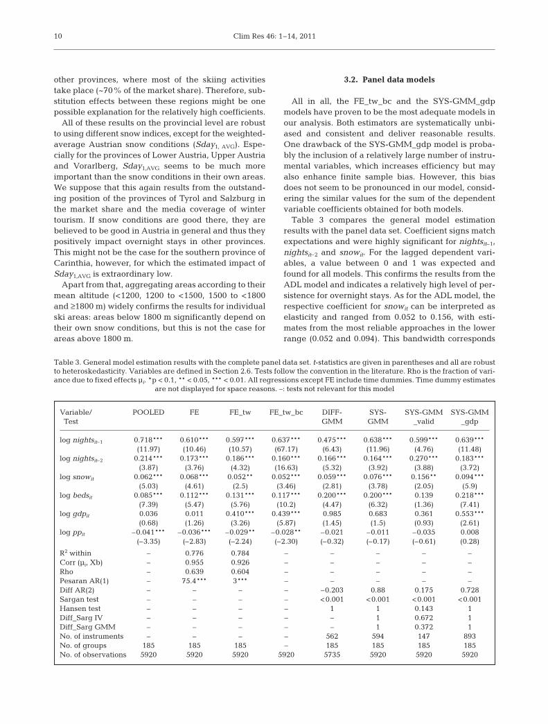
3.2. Panel data models

All in all, the FE_tw_bc and the SYS-GMM_gdpmodels have proven to be the most adequate models inour analysis. Both estimators are systematically unbi-ased and consistent and deliver reasonable results.One drawback of the SYS-GMM_gdp model is proba-bly the inclusion of a relatively large number of instru-mental variables, which increases efficiency but mayalso enhance finite sample bias. However, this biasdoes not seem to be pronounced in our model, consid-ering the similar values for the sum of the dependentvariable coefficients obtained for both models.

Table 3 compares the general model estimationresults with the panel data set. Coefficient signs matchexpectations and were highly significant for nightsit–1,nightsit–2 and snowit. For the lagged dependent vari-ables, a value between 0 and 1 was expected andfound for all models. This confirms the results from theADL model and indicates a relatively high level of per-sistence for overnight stays. As for the ADL model, therespective coefficient for snowit can be interpreted aselasticity and ranged from 0.052 to 0.156, with esti-mates from the most reliable approaches in the lowerrange (0.052 and 0.094). This bandwidth corresponds

10

Variable/ POOLED FE FE_tw FE_tw_bc DIFF- SYS- SYS-GMM SYS-GMMTest GMM GMM _valid _gdp

log nightsit–1 0.718*** 0.610*** 0.597*** 0.637*** 0.475*** 0.638*** 0.599*** 0.639***(11.97) (10.46) (10.57) (67.17) (6.43) (11.96) (4.76) (11.48)

log nightsit–2 0.214*** 0.173*** 0.186*** 0.160*** 0.166*** 0.164*** 0.270*** 0.183***(3.87) (3.76) (4.32) (16.63) (5.32) (3.92) (3.88) (3.72)

log snowit 0.062*** 0.068*** 0.052** 0.052*** 0.059*** 0.076*** 0.156** 0.094***(5.03) (4.61) (2.5) (3.46) (2.81) (3.78) (2.05) (5.9)

log bedsit 0.085*** 0.112*** 0.131*** 0.117*** 0.200*** 0.200*** 0.139 0.218***(7.39) (5.47) (5.76) (10.2) (4.47) (6.32) (1.36) (7.41)

log gdpit 0.036 0.011 0.410*** 0.439*** 0.985 0.683 0.361 0.553***(0.68) (1.26) (3.26) (5.87) (1.45) (1.5) (0.93) (2.61)

log ppit –0.041*** –0.036*** –0.029** –0.028** –0.021 –0.011 –0.035 0.008(–3.35) (–2.83) (–2.24) (–2.30) (–0.32) (–0.17) (–0.61) (0.28)

R2 within – 0.776 0.784 – – – – –Corr (μi, Xb) – 0.955 0.926 – – – – –Rho – 0.639 0.604 – – – – –Pesaran AR(1) – 75.4*** 3*** – – – – –Diff AR(2) – – – – –0.203 0.88 0.175 0.728Sargan test – – – – <0.001 <0.001 <0.001 <0.001Hansen test – – – – 1 1 0.143 1Diff_Sarg IV – – – – – 1 0.672 1Diff_Sarg GMM – – – – – 1 0.372 1No. of instruments – – – – 562 594 147 893No. of groups 185 185 185 – 185 185 185 185No. of observations 5920 5920 5920 5920 5735 5920 5920 5920

Table 3. General model estimation results with the complete panel data set. t-statistics are given in parentheses and all are robustto heteroskedasticity. Variables are defined in Section 2.6. Tests follow the convention in the literature. Rho is the fraction of vari-ance due to fixed effects μi. *p < 0.1, ** < 0.05, *** < 0.01. All regressions except FE include time dummies. Time dummy estimates

are not displayed for space reasons. –: tests not relevant for this model

Töglhofer et al.: Snow conditions and tourism demand

to a 0.6–1.9% change in overnight stays for a 1 SDchange in snow conditions.

The variable bedsit was also highly significant (ex-cept in the SYS-GMM_valid model), which leads us toreject considerations about potential multicollinearity.For the economic variables gdpit and ppit, coefficientswere less reliable and were only significant for somemodel specifications (most notably for the FE_tw andFE_tw_bc models). In particular, relative purchasingpower (ppit) did not seem to play a crucial role in ourmodel, probably owing to the similarity of price devel-opments in Germany, from where most visitors came.Another reason might also be that the CPI has beenused for constructing this variable instead of sometourism price index. Such an index would ideallyinclude regional accommodation, transport and ski liftprices, but this data cannot be obtained for the giventime period and number of observations.

For the variable gdpit, it is interesting to compare thecoefficient of adjustment and the income elasticitiesfrom these 2 models with other panel estimations oftourism demand available in the literature (Garín-Muñoz & Montero-Martín 2007). The coefficient ofadjustment describes the speed of adjustment result-

ing from changes in the exogenous variables. It can beobtained by subtracting the total of the lagged depen-dent variables from 1. Long-term coefficients are thenobtained by dividing (short-term) coefficients with thecoefficient of adjustment. Doing so, we found a rela-tively high short-term robustness with respect to exter-nal effects. The respective model adjustment coeffi-cients of 0.18 and 0.21 show that approximately 20% ofthe adjustment of tourism to changes in the variablestook place within the first 2 yr. The respective long-term income elasticities of 2.18 and 3.01 are in linewith other studies (see Garín-Muñoz & Montero-Martín 2007, Song et al. 2009) and reveal that demandin Austrian ski areas is strongly income elastic, as iscommon for luxury goods.

3.3. Analyzing the temporal evolution

Results for the separate time period panel data mod-els are listed in Table 4. While in the SYS-GMM_gdpmodel the overall trend appears ambiguous for most ofthe variables, a decline in the snowit coefficient can beobserved in the model, from 0.168 in Period 1 to 0.069

11

FE_tw_bc model SYS-GMM_gdp modelVariable/Test Period 1 Period 2 Period 3 Period 1 Period 2 Period 3

log nightsit–1 0.653*** 0.592*** 0.730*** 0.595*** 0.557*** 0.698***(24.83) (19.96) (26.73) (10.53) (5.73) (17.31)

log nightsit–2 0.084*** –0.003 –0.031 0.209** 0.152** 0.122***(3.53) (–0.15) (–1.31) (2.45) (2.21) (3.37)

log snowit 0.087* 0.058** 0.060*** 0.168*** 0.092*** 0.069***(1.9) (2.37) (3.04) (5.22) (3.36) (2.96)

log gdpit 0.875 –0.005 0.515 1.383*** 0.071 0.188(0.95) (–0.03) (0.7) (3.32) (0.29) (1.29)

log bedsit 0.100** 0.255*** 0.245*** 0.232** 0.360** 0.219***(2.24) (5.78) (7.06) (2.39) (2.1) (3.32)

log ppit –0.050*** 0.002 –0.274 –0.004 –0.049 –0.144(–2.80) (0.04) (–1.28) (–0.10) (–1.18) (–1.17)

R2 within 0.62 0.34 0.5 – – –Corr(μi, Xb) 0.95 0.96 0.94 – – –Rho 0.8 0.92 0.9 – – –Pesaran AR(1) 0.73 8.11*** 1.78* – – –Diff AR(2) – – – 0.228 0.128 0.83Sargan test – – – <0.001 <0.001 <0.001Hansen test – – – 0.093 0.987 0.993Diff_(GMM) – – – 0.899 1 1Diff_(IV) – – – 0.358 1 1No. of instruments 0 0 0 136 244 249No. of observations 1850 2035 2035 1850 2035 2035No. of groups 185 185 185 185 185 185Obs. per group 10 11 11 10 11 11

Table 4. Panel data estimation results for the separate time period models. t-statistics are given in parentheses and are all robustto heteroskedasticity. Variables are defined in Section 2.6. Tests follow the convention in the literature. Period 1: 1972/1973–1983/1984 (the lagged dependent variable makes it necessary to dispense with 2 time points). Period 2: 1984/1985–1994/1995.Period 3: 1995/1996–2005/2006. Corr(μi, Xb), R2 within, rho and AR(1) test are obtained from the FE_tw model. Rho is thefraction of variance due to fixed effects μi. *p < 0.1, **p < 0.05, ***p < 0.01. All regressions include time dummies. Time dummy

estimates are not displayed for space reasons. –: tests not relevant for this model

Clim Res 46: 1–14, 2011

in Period 3. The difference is significant at the 10%level. This decline is also confirmed by the variablecoefficient model, where snow coefficients are sub-stantially lower for the last third of the time period.However, in the FE_tw_bc model, this declining trendwas only weakly evident.

The results for the 2 extreme seasons (1989/1990 and2006/2007) also correspond with the results of thepanel data estimations and provide evidence that theimpact of snow poor winters has dramatically de-creased. Although meteorological conditions were sim-ilar in both seasons, the overall change in the growthrate of overnight stays was –8.1 percentage points in1989/1990 and only –2.7 percentage points in 2006/2007. Furthermore, the decrease was more pronouncedin lower-lying areas and no noticeable changes weredetected for higher-lying areas (above 1800 m) or non-skiing areas in either of the two seasons.

4. DISCUSSION

In this section, we discuss 3 issues related to the pre-sented results: the validity of the estimated elasticities,the decrease in the snow sensitivity and the interactionof climate with other factors.

The estimated snow elasticities of demand from timeseries regression and panel data models are wellbelow one, meaning that, in the short-term, overnightstays are inelastic with respect to snow conditions.However, this does not necessarily hold for otherdemand indicators and time horizons, or for extremeseasons. For example, elasticities would probably behigher for direct ski lift tickets sales. Furthermore, inthe long run elasticities are likely to be more pro-nounced, as tourists have time to adapt their behaviourto a long-term change in snow conditions. This meansthat, while impacts are rather limited in the short term,winner–loser patterns might well be observed in thelong term as disadvantaged areas might exit the mar-ket (Elsasser & Bürki 2002, Scott et al. 2006). Apartfrom that, demand response to snow-poor winterseasons might not be linear and elasticities might behigher for extreme seasons. The fact that the residualsin the ski area-specific ADL models are predominantlynegative for the extreme winter season of 1989/1990lends some support to this idea. However, 34 sea-sonal observations are not sufficient to check for non-linearity — a more detailed framework would be re-quired.

One key result of the present study is that snow sen-sitivity of overnight stays decreased substantially inrecent years. This decrease might be attributed tothe major increase in snowmaking and a subsequentdecline in ski area dependency on natural snow cover.

Similar results have also been indicated for the north-eastern US by Dawson et al. (2009). Their climatechange analogue analysis shows that adaptations byski businesses appear to have reduced the impacts ofwarm winters and that, for analogue years, reductionsin season length were lower than those projected insupply-side studies. Of course, other factors such asquality improvements or an increased supply of touristactivities less sensitive to weather conditions mightalso be the reason for this observed trend. At any rate,these effects need to be evaluated more closely forindividual areas, which would require additional in-formation, e.g. data on the start of snowmaking in therespective areas.

Another important question is how the snow riskestimated in the present study is related to other riskfactors for the tourism industry, such as economicconditions, terms of financing or socio-demographicchanges. Economic and meteorological risks are basi-cally uncorrelated, but they may add up at certaintimes. For example, the impacts of the world recessionand economic crisis, such as a decline in sales or atougher bank credit policy, will certainly challenge thetourism industry. This could increase the industry’sexposure to additional risk factors, other than adverseweather conditions, putting the industry also more atrisk from weather-related events.

5. CONCLUSIONS

The objective of the present study was to examinethe impacts of snow conditions on tourism demand inAustrian ski areas on a local scale in the winter seasons1973–2006. Using time series regression and paneldata models, we found a positive relationship betweenovernight stays and snow conditions for the majority ofareas, although higher-lying areas typically showed nodependency on their own snow conditions. However,for some of the higher-lying regions we found a nega-tive dependency of overnight stays on average Aus-trian snow conditions.

Altogether, dependent on the estimation technique,a 1 SD change in snow conditions leads to a 0.6–1.9%change in overnight stays in ski areas, which corre-sponds to 300 000 to 800 000 overnight stays at currentlevels and, for extreme seasons, the impacts might beabove this range. However, we suggest that, at currentlevels of adaptation, impacts should be in the lowerportion of this range, as estimates from the more re-liable approaches point in this direction and the ob-served decrease in sensitivity indicates that snow-poorwinters will have less of an impact compared with pre-vious decades.

A primary objective in climate impact research

12

Töglhofer et al.: Snow conditions and tourism demand

should be to further develop methodological tools tounderstand the impacts of climate variability on eco-nomic activities. As results from our econometric mod-elling show, one step in this direction is to applydynamic time series regression methods or panel datamethods, especially those considered to produce con-sistent and unbiased estimates. Overall, we think thatresults from these approaches are, in general, morerobust than those found in supply-side studies or stud-ies covering single years only, as they allow sensitivi-ties to be compared between different regions and, inparticular, observed over time. For the latter, our workshows that the results crucially depend on the periodunder research (presumably dependent on adaptationlevels) and should, therefore, not be used automati-cally to predict impacts for future time periods withoutfurther analysis.

In summary, our results suggest that although sea-son-to-season variability in weather has a substantialimpact on the industry, in the long term other factorsmay prevail. However, before drawing far-reachingconclusions, a range of other questions need to beaddressed and a closer look at interactions with eco-nomic processes is needed.

Take, for example, the case of snowmaking as a cli-mate adaptation strategy. Its increased utilizationreduces the exposure of ski areas towards naturalsnow conditions, but this positive effect could be offsetin the longer term by a negative impact of price elastic-ity of demand. An evaluation of this counter effectrequires better understanding of how price changesinfluence ski tourism as well as an analysis of theextent to which the costs of snowmaking investmentshave been passed directly on to consumers (or taxpay-ers, as some regions were subsidizing this kind ofinvestment) rather than being covered by revenuesfrom additional demand. Furthermore, when relativeprice changes become important factors explainingchanges within tourism, a macroeconomic frameworkis needed, e.g. computed general equilibrium model-ling. From an economic point of view, further researchshould go in this direction, particularly as recent workindicates that, although even at lower altitudes snowmaking might climatically still be possible under a 2°Cwarming scenario, its intensified application will leadto significantly higher operation costs (Steiger & Mayer2008).

In addition, any change in tourism demand mighthave broader implications for the Austrian economy.Although this was not the focus of the present study,Prettenthaler et al. (2009) examined the impacts of auniform 10% decrease in overnight stays in the winterseason and showed that the overall macroeconomiceffect in terms of GDP doubled the initial demandshock to tourism. Their results suggest that the most

important negative macroeconomic effects are not tobe borne by the tourism-intensive provinces such asTyrol and Salzburg, but by Upper and Lower Austria,with their high share in the food industry and othersectors that deliver to the tourism sector. Thus, bothlines of research, the macroeconomic approach justmentioned as well as the microeconomic approach wehave presented in this paper, point to the importanceof the regional scale in the further development of inte-grated economic assessment models of climate changeimpacts and adaptation.

Acknowledgements. Major parts of this research were gener-ously supported by the Jubiläumsfonds of the ÖNB (CentralBank of the Republic of Austria). C.T. received a researchgrant from the URBI faculty of the University of Graz. Theauthors also thank B. Bednar-Friedl, A. Gobiet, H. Gurgul, J.Köberl, R. Mestel, R. Potzmann, S. Schiman, W. Schöner, K.Steininger, M. Themessl and 3 anonymous reviewers for valu-able contributions and helpful comments on this work.

LITERATURE CITED

Abegg B, Agrawala S, Crick F, de Montfalcon A (2007) Cli-mate change impacts and adaptation in winter tourism. In:Agrawala S (ed) Climage change in the European Alps:Adapting winter tourism and natural hazards manage-ment. Organization for Economic Cooperation and Devel-opment, Paris, p 25–58

Agnew MD, Palutikof JP (2006) Impacts of short-term climatevariability in the UK on demand for domestic and interna-tional tourism. Clim Res 31:109–120

Arellano M, Bond S (1991) Some tests of specification forpanel data: Monte Carlo evidence and an application toemployment equations. Rev Econ Stud 58:277–297

Arellano M, Bover O (1995) Another look at the instrumentalvariable estimation of error-component models. J Econom68:29–51

Baltagi BH (2008) Econometric analysis of panel data, 4thedn. John Wiley, Chichester

Beck A, Hiebl J, Koch E, Potzmann R, Schöner W (2009) Insti-tutionelle und regulatorische Fragestellungen der Bereit-stellung von Wetterdaten. Economics of Weather and Cli-mate Risks Working Paper Series 10/2009, JohanneumResearch, Graz. Available at www.klimarisiko.at/node/42

bergfex (2009) Austrian ski areas. Available at www.bergfex.at/BEV (Bundesamt für Eich- und Vermessungswesen) (2009)

Austrian Map 3D Software. BEV, ViennaBigano A, Goria A, Hamilton JM, Tol RSJ (2005) The effect of

climate change and extreme weather on tourism. In:Lanza A, Markandya A, Pigliaru F (eds) The economics oftourism and sustainable development. Edward Elgar,Cheltenham

Bigano A, Hamilton JM, Tol RSJ (2006) The impact of climateon holiday destination choice. Clim Change 76:389–406

Blundell R, Bond S (1998) Initial conditions and momentrestrictions in dynamic panel data models. J Econom 87:115–143

Breiling M, Charamza P (1999) The impact of global warmingon winter tourism and skiing: a regionalised model forAustrian snow conditions. Reg Environ Change 1:4–14

Breusch TS (1978) Testing for autocorrelation in dynamic lin-ear models. Aust Econ Pap 17:334–355

13

Clim Res 46: 1–14, 2011

Breusch TS, Pagan AR (1979) Simple test for heteroscedastic-ity and random coeffcient variation. Econometrica 47:1287–1294

Bruno GSF (2005) Estimation and inference in dynamicunbalanced panel-data models with a small number ofindividuals. Stata J 5:473–500

Dawson J, Scott D, McBoyle G (2009) Climate change ana-logue analysis of ski tourism in the northeastern USA.Clim Res 39:1–9

Elsasser H, Bürki R (2002) Climate change as a threat totourism in the Alps. Clim Res 20:253–257

Fukushima T, Kureha M, Ozaki N, Fukimori Y, Harasawa H(2002) Influences of air temperature change on leisureindustries: case study on ski activities. Mitig Adapt StratGlob Change 7:173–189

Galloway RW (1988) The potential impact of climate changeson Australian ski fields. In: Pearmann GI (ed) Green-house: planning for climate change. CSIRO, Melbourne,p 428–437

Garín-Muñoz T, Montero-Martín LF (2007) Tourism in theBalearic Islands: a dynamic model for international de-mand using panel data. Tour Manag 28:1224–1235

Godfrey LG (1978) Testing against general autoregressiveand moving average error models when the regressorsinclude lagged dependent variables. Econometrica 46:1293–1302

Hamilton JM, Maddison DJ, Tol RSJ (2005) Climate changeand international tourism: a simulation study. Glob Envi-ron Change 15:253–266

Hamilton LC, Brown C, Keim BD (2007) Ski areas, weatherand climate: Time series models for New England casestudies. Int J Climatol 27:2113–2124

Harrison R, Kinnaird V, McBoyle G, Quinlan C, Wall G (1986)Recreation and climate change: a Canadian case study.Ontario Geogr 23:51–68

Hennessy KJ, Whetton PH, Walsh K, Smith IN, Bathols JM,Hutchinson M, Sharples J (2008) Climate change effectson snow conditions in mainland Australia and adaptationat ski resorts through snowmaking. Clim Res 35:255–270

Jarque CM, Bera AK (1980) Efficient tests for normality,homoscedasticity and serial independence of regressionresiduals. Econ Lett 6:255–259

Joanneum Research (2008) Austrian ski resort database.JOANNEUM Research, Institute of Technology and Re-gional Policy, Graz

König U, Abegg B (1997) Impacts of climate change on wintertourism in the Swiss Alps. J Sustain Tourism 5:46–58

Laimer P, Smeral E (2006) Ein Tourismus-Satellitenkonto fürÖsterreich: Methodik, Ergebnisse und Prognosen für dieJahre 2000 bis 2007. Statistics Austria and WIFO (AustrianInstitute for Economic Research), Vienna

Lamothe & Périard Consultants (1988) Implications of climatechange for downhill skiing in Quebec. Climate ChangeDigest 88-03. Environment Canada, Ottawa

Lipski S, McBoyle G (1991) The impact of global warming ondownhill skiing in Michigan. East Lakes Geogr 26:37–51

Lise W, Tol RSJ (2002) Impact of climate on tourist demand.Clim Change 55:429–449

Luzzi GF, Flückiger Y (2003) An econometric estimation of thedemand for tourism: the case of Switzerland. Pac Econ Rev8:289–303

Maddison D (2001) In search of warmer climates? The impactof climate change on flows of British tourists. Clim Change49:193–208

McBoyle G, Wall G (1992) Great Lakes skiing and climatechange. In: Gill A, Hartman R (ed) Mountain resort devel-opment. Simon Fraser University, Centre for Tourism Pol-icy and Research, Burnaby, p 71–81

Nickell SJ (1981) Biases in dynamic models with fixed effects.Econometrica 49:1417–1426

OECD (2008) Consumer price index and gross domesticproduct. OECD, available at http://stats.oecd.org/

Prettenthaler F, Formayer H, Aumayer Ch, Haas P and others(2009) Global Change Impact on Tourism: Der sozioöko-nomische Einfluss des Klimawandels auf den Winter- undSommertourismus in Österreich. Joanneum Research, Graz

Ramsey JB (1969) Tests for specification errors in classical lin-ear least squares regression analysis. J R Stat Soc A 31:350–371

Roodman D (2009) How to do xtabond2: an introduction to‘Difference’ and ‘System’ GMM in Stata. Stata J 9:86–136

Scott D, McBoyle G, Mills B (2003) Climate change and theskiing industry in southern Ontario (Canada): exploringthe importance of snowmaking as a technical adaptation.Clim Res 23:171–181

Scott D, McBoyle G, Minogue A, Mills B (2006) Climate changeand the sustainability of ski-based tourism in eastern NorthAmerica: a reassessment. J Sustain Tourism 14:376–398

Scott D, Dawson J, Jones B (2008) Climate change vulnerabil-ity of the US Northeast winter recreation-tourism sector.Mitig Adapt Strategies Glob Change 13:577–596

Sequeira N, Nunes P (2008) Does country risk influence inter-national tourism? A dynamic panel data analysis. EconRec 84:223–236

Shih C, Nicholls S, Holecek DF (2009) Impact of weather ondownhill ski lift ticket sales. J Travel Res 47:359–372

Song H, Witt SF, Li G (2009) The advanced econometrics oftourism demand. Routledge, New York

Statistics Austria (2008) Overnight stays in Austrian munici-palities in the winter season 1973 to 2007. Statistics Austria,Vienna

Steiger R, Mayer M (2008) Snowmaking and climate change:future options for snow production in Tyrolean ski resorts.Mt Res Dev 28:292–298

Teich M, Lardelli C, Bebi P, Gallati D and others (2007) Klima-wandel und Wintertourismus: Ökonomische und ökologi-sche Auswirkungen von technischer Beschneiung. Eidg.Forschungsanstalt für Wald, Schnee und Landschaft, Bir-mensdorf

ZAMG (Central Institute for Meteorology and Geodynamics)(2009) 1 × 1 km grid data for air temperature, precipitationand snow 1948–2006. ZAMG, Vienna

14

Editorial responsibility: Helmut Mayer,Freiburg, Germany

Submitted: April 22, 2010; Accepted: September 20, 2010Proofs received from author(s): December 24, 2010