impact of top-surface morphology on co storage capacity
TRANSCRIPT
Impact of top-surface morphology on CO2 storage
capacityI
Halvor Møll Nilsena, Anne Randi Syversveenb, Knut-Andreas Liea,d, JanTverangerc, Jan M. Nordbottend
aSINTEF ICT, PO Box 124, Blindern, N-0314 Oslo, NorwaybNorwegian Computing Center, PO Box 114, Blindern, N-0314 Oslo, Norway
cCenter for Integrated Petroleum Research, Uni Research, PO Box 7800, N-5020 Bergen,Norway
dDepartment of Mathematics, University of Bergen, PO Box 7800, N-5020 Bergen,Norway
Abstract
Long-term forecasting of the behaviour of CO2 injected in industrial quanti-ties into sub-surface reservoirs is generally performed using models includingvery limited geological detail. This practise, although dictated by restrictionswith respect to model resolution and CPU cost, partly rests on an unverifiedbut widely held assumption that geological detail will not influence simu-lation outcomes on the spatial and temporal scales relevant for geologicalsequestration. The present study aims to partly assess the validity of thisassumption by selecting a series of realistic geological features and investigatetheir impact when modelling CO2 sequestration.
Injected CO2 is primarily retained in structural and stratigraphic trapsat the top of the reservoir interval. We will therefore investigate how dif-ferent top-surface morphologies will influence the CO2 storage capacity. Tothis end, a series of different top surfaces are created by combining differentstratigraphic scenarios with different structural scenarios. The models arecreated stochastically to quantify uncertainty. Theoretical upper bounds onthe volume available for structural trapping are established by a geometricalanalysis. Estimates for actual trapping from a single point source are calcu-lated in a simplified and efficient manner by a spill-point analysis and more
IThe full data sets and additional illustrations are available from the IGEMS webpage:http://igems.nr.no/
Preprint submitted to International Journal of Greenhouse Gas Control August 26, 2012

accurately by a detailed flow simulation that assumes vertical equilibrium.Results from the two approaches are compared. For the fluid flow simulationmethod, we investigate the effect of grid resolution. The experiments showthat the morphology of the top seal is of great importance for the storagecapacity and migration patterns and that the effect of upscaling is highlystructure dependent.
Keywords: structural trapping, spill point analysis, upscaling, uncertaintyanalysis
1. Introduction
To reduce carbon emissions to the atmosphere, storing CO2 in deep sub-surface rock formations has become an important issue. Most of the technol-ogy required to inject and store CO2 in saline aquifers, unminable coal seams,or abandoned petroleum reservoirs is already available from the petroleumand mining industry. The main question is the cost and risk associated withthe storage operation. Three elements are essential to consider CO2 storagein a specific location. First, there must be sufficient pore volume to store allthe CO2. Second, there must be an intact top-seal to ensure containment,and, finally, injection should be possible within operational constraints.
A significant number of research projects involving field testing of sub-surface CO2 storage exist worldwide (see www.ieaghg.org). The main pur-pose of most of these studies is to investigate practical and technical chal-lenges related to sequestering CO2 in underground formations. None of thesepractical tests involve volumes, rates, and time scales approaching the en-visaged requirements for long-term geological storage of gigatonnes of CO2.Assessments of feasibility and safety of long-term storage of significant vol-umes of CO2 at a particular site must be based on reliable, model-based fore-casting of sub-surface behaviour of CO2. Models employed for this purposeshould ideally include all parameters likely to affect the outcome. Neverthe-less, in this context many geological parameters are overlooked, ignored orconsidered to have insignificant impact at temporal and spatial scales rele-vant to geological storage of CO2. There is an obvious need to address thehandling and implementation of geological parameters and their impact onCO2 sequestration in a methodical manner. This will in turn give constraintswith respect to which parameters should be included in large-scale, long-termsimulation of CO2 sequestration.
2

Site characterisation for sequestration purposes on an industrial scalelargely centres on establishing storage capacity, injectivity potential, CO2
interaction with the surrounding rocks and fluids, and assessing contain-ment and potentially detrimental impact on natural resources. To this end,comprehensive numerical simulation capabilities have been developed (Celiaet al., 2010; Class et al., 2009), but academic studies and community bench-marks of CO2 injection have so far largely focused on numerical and modelling-based uncertainties (Pruess et al., 2004; Class et al., 2009), employing con-ceptual or highly simplified representations of subsurface geology and givinglittle attention to uncertainties originating from formation properties. Inparticular, we are missing systematic studies that investigate and develop ageneric quantitative understanding of how formation properties and geome-tries impact large-scale CO2 sequestration. Such studies would, in turn, allowqualified simplification of models by offering an “impact-ranking” of param-eters and focus data collection for modelling purposes towards prioritisingcollection of data related to high-impact geological parameters.
Herein, we make a first step in this direction by considering a syntheticstorage scenario in which the reservoir consists of good quality sand buriedunderneath an impermeable caprock that dips slightly in one direction. Su-percritical CO2 is a buoyant fluid, and after injection, it moves upwards, untilencountering a barrier that prevents further movement. Then the fluid moveslaterally upslope along the barrier until the end of the barrier or a trap isreached, where accumulation can take place. In particular, this means thatthe morphology of the top seal will affect CO2 migration pathways, shapeand size of traps, and the seal integrity on reservoir scale. In the following,we assume that top-surface morphology is the main driver of uncertainty.Using a simple model setup with virtually uniform properties but variabletop-surface topography, we study how different reliefs in this morphologyimpact estimates of storage capacity and migration patterns. To this end,multiple geostatistical realisations of each sedimentological scenario are re-quired to quantify the relative uncertainty associated with depositional andstructural architecture and their associated petrophysical properties.
In the following, we outline the selection of the geological features chosenin our study, describe the overall design of our model set-up for studyingtheir impact on CO2 sequestration, briefly discuss generation of geostatisticalrealisations, present simulation results, and discuss the effects of upscalingto determine how much the models can upscaled without losing importantdetails
3

2. Selection of geological features
Geological storage of CO2 benefits from experiences gained and toolsdeveloped by the petroleum industry over many decades, in particular withrespect to subsurface data acquisition and handling, the use of reservoir mod-elling tools and methods for discretizing and quantifying geological featuresand properties from wells, seismic data and outcrop analogues. Fluid-flowsimulation of hydrocarbon reservoirs also routinely involves assessing the in-terplay between geology and reservoir behaviour. However, despite obvioussimilarities with respect to the common need for a comprehensive under-standing of formation properties, subsurface characterisation for large-scaleCO2 sequestration needs to consider a number of aspects normally not viewedas important in petroleum production models. The life-span of a producingpetroleum reservoir is a few decades at most, focusing modelling towardsconsidering reservoir dynamics and processes operating on a relatively shorttime scale. Regulations for CO2 sequestration, on the other hand, stipulateforecasting on a scale of thousands of years, which implies taking into accounta number of slow-acting processes such as tectonic movements, glaciations,sea level changes, and slow chemical reactions between the injected CO2,pore-fluids, and rock. A further contrast is presented by spatial scale. Mosthydrocarbon fields cover less than few tens square kilometres, whereas someplanned CO2 injection schemes envisage sequestration in formations coveringseveral thousand square kilometres. To cut CPU cost, these contrasts in tem-poral and spatial scale are often taken as an argument in favour of employingsimplified geological models when simulating long-term, large-scale CO2 in-jection. However, the underlying assumption, that geological features provenimportant in hydrocarbon production may have a negligible impact on thescales employed for CO2 sequestration, remains largely unsubstantiated asrelevant studies are lacking.
The basic concept of the present study is broadly based on the approachtaken by the SAIGUP project (Manzocchi et al., 2008), which ventured toassess the influence of geological factors on production by analysing a largesuite of synthetic models generated by combining sedimentological modelsranging from comparatively simple to highly complex with a series of struc-tural scenarios. Our original intention to re-run parts of the SAIGUP modelmatrix, replacing petroleum production with CO2 injection, had to be aban-doned as the size of the SAIGUP model template (3.0 km × 9.0 km × 80m) turned out to be too small, causing the injected CO2 to migrate out of
4
the model area within a few years of simulation time, e.g., as discussed byAshraf et al. (2010). Consequently a new model template had to be gener-ated for the purpose of this study. It covers an area of 30 by 60 km andincludes a 100 m thick reservoir unit. The overall shape is slightly convexand tilted one degree along its long-axis in order to control plume movementduring simulation. The top of the reservoir is envisaged as capped by thick,impermeable shale and thus not explicitly included in our models.
To limit the scope of the present study, we decided to focus on a setof geological features in siliciclastic rocks that straddle seismic resolution interms of scale and with a proven but as yet not systematically studied impacton CO2 sequestration. Top reservoir topography fulfils this criterion as it hasbeen observed to have a significant impact on CO2 migration on 4D seismicdata (Chadwick and Noy, 2010; Chadwick et al., 2010; Eiken et al., 2011),whereas its potential impact on sub-seismic scale has not been studied.
Geological features affecting the topography of the reservoir/seal interfaceare commonly only included in reservoir models if they have been explicitlymapped on seismic surveys. In general this implies that features with reliefamplitudes below seismic resolution (i.e., about 10–15 m) are not capturedexplicitly in reservoir models (although sub-seismic faults may occasionallybe included). Thus top reservoir topography, as seen in most reservoir mod-els, is largely defined by tectonic features such as faults exceeding 10–15 m ofdisplacement, and large-scale folding and tilting. This simplifies or overlooksthe fact that top reservoir topography at or below seismic resolution can beaffected by a number of factors such as draped or in-filled depositional orerosional relief, sub-seismic scale faults, laterally non-uniform compaction,various forms of diapirism and breccia pipes.
3. Geological features
We selected a series of depositional, erosional and tectonic features ac-cording to a set of criteria governed by our chosen horizontal model reso-lution of 100m × 100m and the overall requirement of providing “realistic”scenarios. Our choice of model resolution was influenced by the need to keepcomputational cost of the simulations within practical limits.
To match the scale and resolution of our model, we focus on geologicalfeatures with reasonably predictable properties in terms of scales, geometriesand distribution patterns and with a potential to produce recurrent and pre-dictable spatial patterns in an area of 30 km by 60 km. Although features
5
such as diapirs, sand dykes, and breccia pipes can substantially influencetop-reservoir configurations and integrity, their seismic and sub-seismic char-acteristics in terms of size, and spatial distribution on scales similar to ourmodel area is poorly constrained by empirical data sets. The resulting lack ofcontrol of realistic model input parameters poses a problem when evaluatingthe generic influence of such features on fluid simulation outcomes.
A final requirement defined by the project was the “stratigraphic real-ism” of the features to be included in the model: Stratigraphic successionsinvolving thick, impermeable shale sealing an underlying sandy reservoir unit,(forming our basic model set-up), are commonly products of substantial sea-level rise forcing a regional shift from sand to shale deposition. The chosengeological features influencing top reservoir topography should therefore bestructures known to or expected to occur at such stratigraphic positions.
The chosen sedimentological features include: 1) buried beach ridges in aflooded marginal marine setting (FMM), and 2) buried offshore sand ridges(OSS). Both fulfil the above stated criteria by being resolvable features onthe chosen modelling scale, straddling seismic resolution, having geometriesand spatial distributions constrained by empirical data, and occur or mayoccur at the interface between a sandy reservoir unit and an overlying thickimpermeable shale unit.
Buried beach ridges in a flooded marginal-marine setting (FMM). Beachridges are defined as relict, semiparallel, multiple ridges, either wave (bermridge) or wind (multiple backshore foredune) origin and usually formingstrandplains Otvos (2000). They originate in the inter- and supratidal zoneand may consist of either siliciclastic or calcareous material ranging fromfine sand to cobbles and boulders. Strandplains with systems of more or lessevenly spaced beach ridges commonly reflect forced shoreline progradation orfalling relative sea level (e.g., Curray and Moore (1964); Nielsen and Johan-nessen (2001)) and can cover extensive areas. Ridges influenced by aeolianprocesses may produce a relief of 8 m or more (Stapor et al., 1991).
Due to their low relief, beach ridges are difficult to identify in anything buthigh resolution seismic data. Seismic attribute maps from the lower BrentGroup in the North Sea (Jackson et al., 2010) revealed an extensive systemof beach ridges preserved at the boundary between the shallow marine EtiveFm. and the overlying Ness Fm. suggesting that these features may be morefrequent in the fossil record than previously envisaged. Key morphometricdimension of beach ridge systems used in our study are shown in Table 1.
6
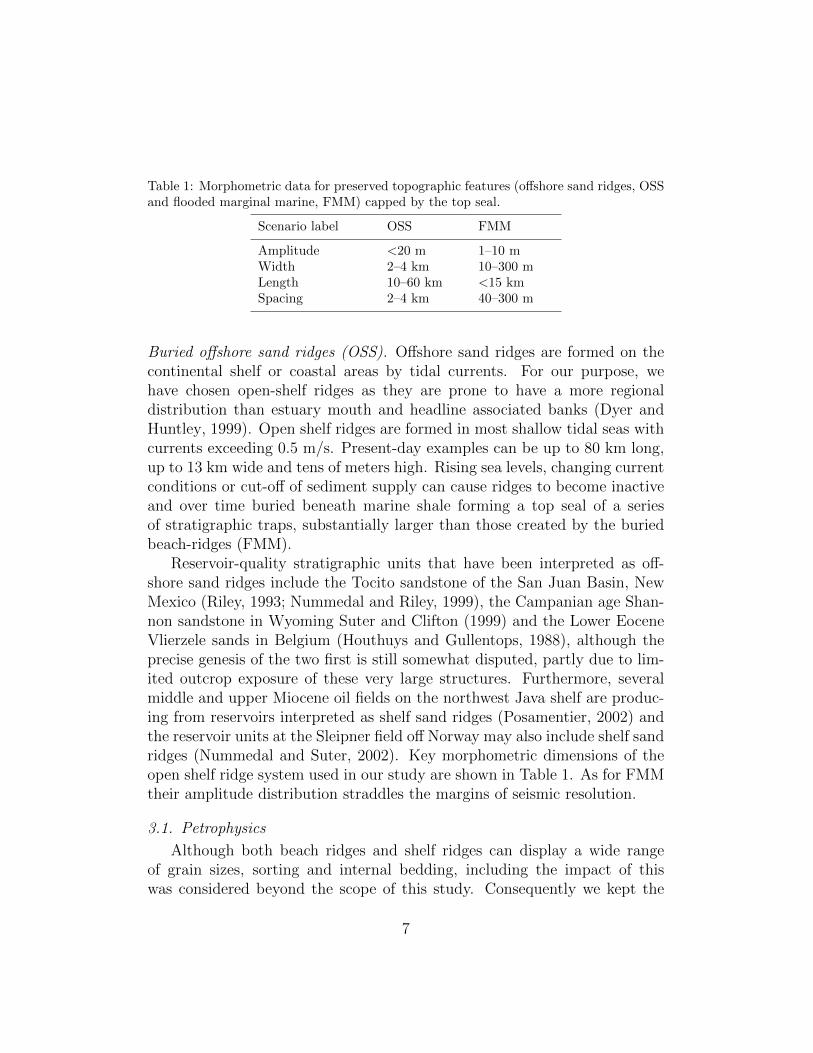
Table 1: Morphometric data for preserved topographic features (offshore sand ridges, OSSand flooded marginal marine, FMM) capped by the top seal.
Scenario label OSS FMM
Amplitude <20 m 1–10 mWidth 2–4 km 10–300 mLength 10–60 km <15 kmSpacing 2–4 km 40–300 m
Buried offshore sand ridges (OSS). Offshore sand ridges are formed on thecontinental shelf or coastal areas by tidal currents. For our purpose, wehave chosen open-shelf ridges as they are prone to have a more regionaldistribution than estuary mouth and headline associated banks (Dyer andHuntley, 1999). Open shelf ridges are formed in most shallow tidal seas withcurrents exceeding 0.5 m/s. Present-day examples can be up to 80 km long,up to 13 km wide and tens of meters high. Rising sea levels, changing currentconditions or cut-off of sediment supply can cause ridges to become inactiveand over time buried beneath marine shale forming a top seal of a seriesof stratigraphic traps, substantially larger than those created by the buriedbeach-ridges (FMM).
Reservoir-quality stratigraphic units that have been interpreted as off-shore sand ridges include the Tocito sandstone of the San Juan Basin, NewMexico (Riley, 1993; Nummedal and Riley, 1999), the Campanian age Shan-non sandstone in Wyoming Suter and Clifton (1999) and the Lower EoceneVlierzele sands in Belgium (Houthuys and Gullentops, 1988), although theprecise genesis of the two first is still somewhat disputed, partly due to lim-ited outcrop exposure of these very large structures. Furthermore, severalmiddle and upper Miocene oil fields on the northwest Java shelf are produc-ing from reservoirs interpreted as shelf sand ridges (Posamentier, 2002) andthe reservoir units at the Sleipner field off Norway may also include shelf sandridges (Nummedal and Suter, 2002). Key morphometric dimensions of theopen shelf ridge system used in our study are shown in Table 1. As for FMMtheir amplitude distribution straddles the margins of seismic resolution.
3.1. Petrophysics
Although both beach ridges and shelf ridges can display a wide rangeof grain sizes, sorting and internal bedding, including the impact of thiswas considered beyond the scope of this study. Consequently we kept the
7
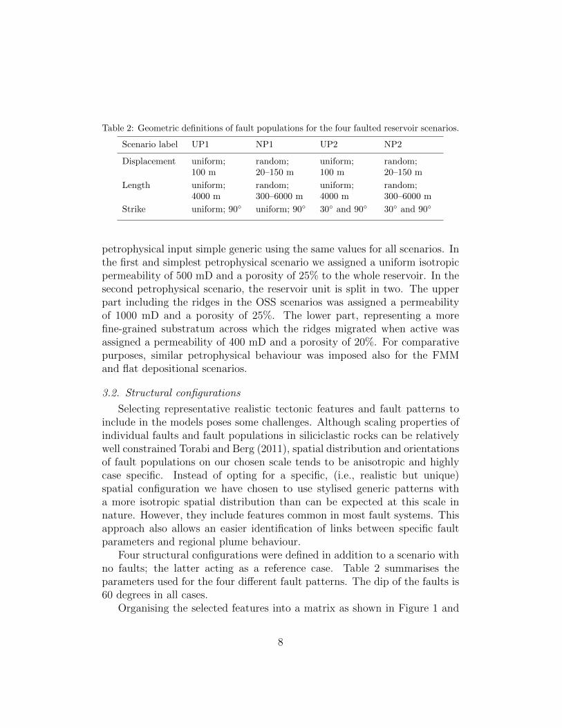
Table 2: Geometric definitions of fault populations for the four faulted reservoir scenarios.
Scenario label UP1 NP1 UP2 NP2
Displacement uniform;100 m
random;20–150 m
uniform;100 m
random;20–150 m
Length uniform;4000 m
random;300–6000 m
uniform;4000 m
random;300–6000 m
Strike uniform; 90◦ uniform; 90◦ 30◦ and 90◦ 30◦ and 90◦
petrophysical input simple generic using the same values for all scenarios. Inthe first and simplest petrophysical scenario we assigned a uniform isotropicpermeability of 500 mD and a porosity of 25% to the whole reservoir. In thesecond petrophysical scenario, the reservoir unit is split in two. The upperpart including the ridges in the OSS scenarios was assigned a permeabilityof 1000 mD and a porosity of 25%. The lower part, representing a morefine-grained substratum across which the ridges migrated when active wasassigned a permeability of 400 mD and a porosity of 20%. For comparativepurposes, similar petrophysical behaviour was imposed also for the FMMand flat depositional scenarios.
3.2. Structural configurations
Selecting representative realistic tectonic features and fault patterns toinclude in the models poses some challenges. Although scaling properties ofindividual faults and fault populations in siliciclastic rocks can be relativelywell constrained Torabi and Berg (2011), spatial distribution and orientationsof fault populations on our chosen scale tends to be anisotropic and highlycase specific. Instead of opting for a specific, (i.e., realistic but unique)spatial configuration we have chosen to use stylised generic patterns witha more isotropic spatial distribution than can be expected at this scale innature. However, they include features common in most fault systems. Thisapproach also allows an easier identification of links between specific faultparameters and regional plume behaviour.
Four structural configurations were defined in addition to a scenario withno faults; the latter acting as a reference case. Table 2 summarises theparameters used for the four different fault patterns. The dip of the faults is60 degrees in all cases.
Organising the selected features into a matrix as shown in Figure 1 and
8

←−
Increa
singco
mplexityof
sedim
entary
topography
Increasing structural complexity −→0 UP1 NP1 UP2 NP2
Flat
OSS
FMM
Figure 1: Overview in terms of a heterogeneity matrix for the selected geological features.
running the resulting combinations of structural and sedimentary featuresallows us to identify the impact of each combination by comparing it to abase case (smooth top reservoir and no faults).
3.3. Stochastic modelling
The geological base-case scenarios described above are modelled by geo-statistical methods. In this way, the uncertainty within each model can beexplored. A set of top surfaces were generated as follows. First, a base-casesurface measuring 30×60 km, with a height difference of 500 meters betweenthe two short ends was created. It has the ideal shape of an inverse half pipeparallel to the longest axis to avoid or minimise leakage over the long edges.The depth of the shallowest point is below 1000 meters to ensure that theCO2 remains a supercritical phase. The top surfaces of the OSS and FMMmodels were created by Gaussian random fields and added on top of thebase case surface. For both OSS and FMM, a sinusoidal covariance of formsin(x)/x was used. For OSS, the range along the long axis was 1000 meters,reflecting the width of the lobes, and the range along the short axis was 7000meters, reflecting the length of the lobes. The standard deviation is 13 me-ters, reflecting the height of the lobes. For the FMM case, the ranges were200 meters along the long axis and 700 meters along the short axis, and thestandard deviation was 5 meters. This gives us three different stratigraphicmodels: the base case with flat deposition, offshore sand ridges (OSS), and
9

Figure 2: Top surfaces: the left plot shows offshore sand ridges (OSS) and the right plotshows a flooded marginal marine (FMM) deposition.
flooded marginal marine (FMM). These three stratigraphic models were allcombined with the four different structural models. The structural modelswere modelled by the fault modelling tool Havana (Hollund et al., 2002),which is based on a marked point model, using the parameters given in Ta-ble 2. Altogether, two hundred faults were generated for each of the models.The combination of stratigraphic and structural models gives us in totalfifteen different models; the three stratigraphic models without faults, andeach of them combined with four different fault patterns. For each model,except for the base model without faults, 100 realisations were generated andcan be downloaded from the IGEMS website (IGEMS, 2011). Examples ofsimulated top surfaces are shown in Figure 2.
4. Estimation of storage capacity
We consider a simple scenario in which CO2 is injected from a singlewell. During injection, the main concern is the pressure build-up during theformation of the CO2 plume. The top-surface morphology is unlikely to havesignificant impact on pressure build-up during injection, and herein we willtherefore mainly focus on how the morphology affects the degree of structuraltrapping and the general long-term migration of the CO2 plume.
Full 3D simulation of several thousand years of plume migration in a30 × 60 km2 reservoir model with a lateral resolution of 100 × 100 m2 hasa prohibitive computational cost. In this section, we will therefore considertwo simplified methods for estimating storage capacity.
4.1. Structural trapping capacity
To estimate the upper theoretical capacity for structural trapping, we willuse a geometric analysis to identify the cascade of structural traps associated
10
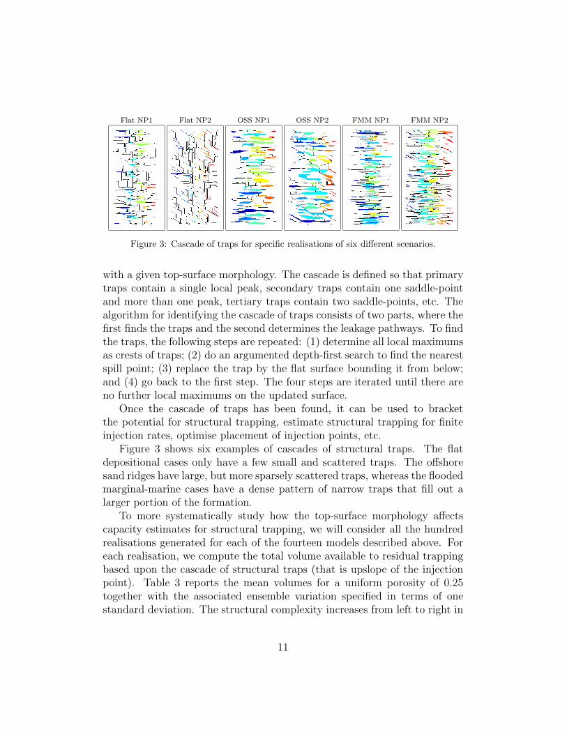
Flat NP1 Flat NP2 OSS NP1 OSS NP2 FMM NP1 FMM NP2
Figure 3: Cascade of traps for specific realisations of six different scenarios.
with a given top-surface morphology. The cascade is defined so that primarytraps contain a single local peak, secondary traps contain one saddle-pointand more than one peak, tertiary traps contain two saddle-points, etc. Thealgorithm for identifying the cascade of traps consists of two parts, where thefirst finds the traps and the second determines the leakage pathways. To findthe traps, the following steps are repeated: (1) determine all local maximumsas crests of traps; (2) do an argumented depth-first search to find the nearestspill point; (3) replace the trap by the flat surface bounding it from below;and (4) go back to the first step. The four steps are iterated until there areno further local maximums on the updated surface.
Once the cascade of traps has been found, it can be used to bracketthe potential for structural trapping, estimate structural trapping for finiteinjection rates, optimise placement of injection points, etc.
Figure 3 shows six examples of cascades of structural traps. The flatdepositional cases only have a few small and scattered traps. The offshoresand ridges have large, but more sparsely scattered traps, whereas the floodedmarginal-marine cases have a dense pattern of narrow traps that fill out alarger portion of the formation.
To more systematically study how the top-surface morphology affectscapacity estimates for structural trapping, we will consider all the hundredrealisations generated for each of the fourteen models described above. Foreach realisation, we compute the total volume available to residual trappingbased upon the cascade of structural traps (that is upslope of the injectionpoint). Table 3 reports the mean volumes for a uniform porosity of 0.25together with the associated ensemble variation specified in terms of onestandard deviation. The structural complexity increases from left to right in
11
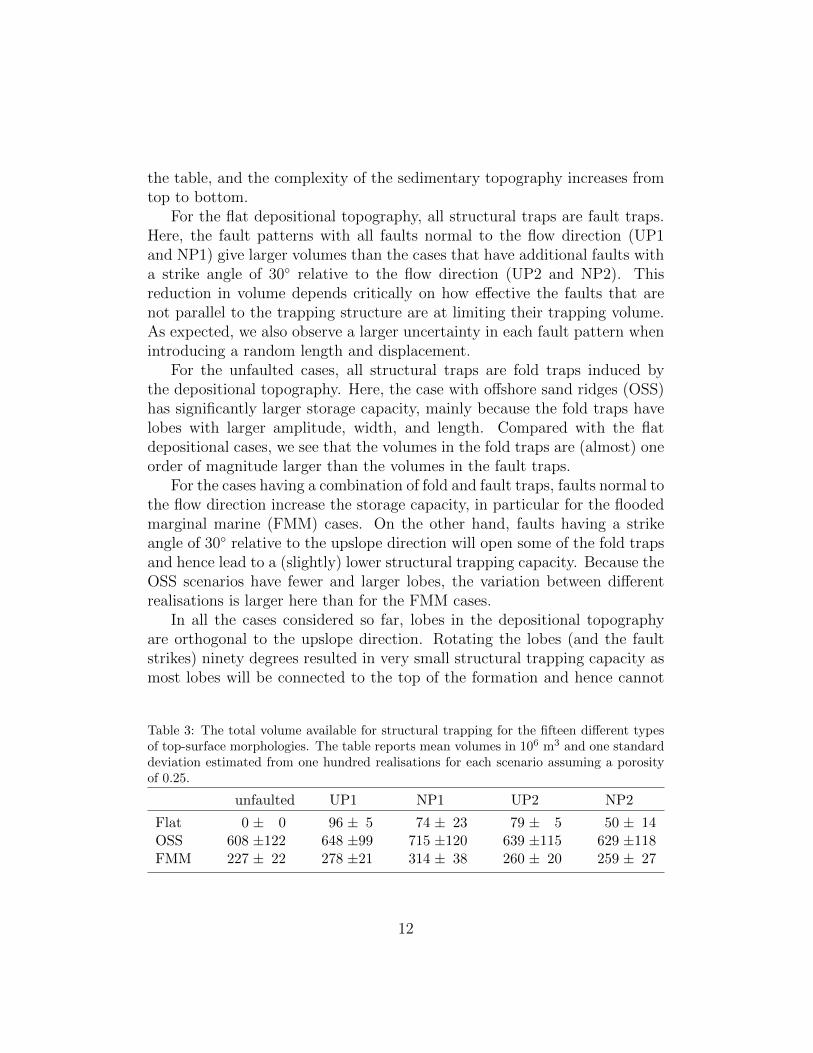
the table, and the complexity of the sedimentary topography increases fromtop to bottom.
For the flat depositional topography, all structural traps are fault traps.Here, the fault patterns with all faults normal to the flow direction (UP1and NP1) give larger volumes than the cases that have additional faults witha strike angle of 30◦ relative to the flow direction (UP2 and NP2). Thisreduction in volume depends critically on how effective the faults that arenot parallel to the trapping structure are at limiting their trapping volume.As expected, we also observe a larger uncertainty in each fault pattern whenintroducing a random length and displacement.
For the unfaulted cases, all structural traps are fold traps induced bythe depositional topography. Here, the case with offshore sand ridges (OSS)has significantly larger storage capacity, mainly because the fold traps havelobes with larger amplitude, width, and length. Compared with the flatdepositional cases, we see that the volumes in the fold traps are (almost) oneorder of magnitude larger than the volumes in the fault traps.
For the cases having a combination of fold and fault traps, faults normal tothe flow direction increase the storage capacity, in particular for the floodedmarginal marine (FMM) cases. On the other hand, faults having a strikeangle of 30◦ relative to the upslope direction will open some of the fold trapsand hence lead to a (slightly) lower structural trapping capacity. Because theOSS scenarios have fewer and larger lobes, the variation between differentrealisations is larger here than for the FMM cases.
In all the cases considered so far, lobes in the depositional topographyare orthogonal to the upslope direction. Rotating the lobes (and the faultstrikes) ninety degrees resulted in very small structural trapping capacity asmost lobes will be connected to the top of the formation and hence cannot
Table 3: The total volume available for structural trapping for the fifteen different typesof top-surface morphologies. The table reports mean volumes in 106 m3 and one standarddeviation estimated from one hundred realisations for each scenario assuming a porosityof 0.25.
unfaulted UP1 NP1 UP2 NP2
Flat 0 ± 0 96 ± 5 74 ± 23 79 ± 5 50 ± 14OSS 608 ±122 648 ±99 715 ±120 639 ±115 629 ±118FMM 227 ± 22 278 ±21 314 ± 38 260 ± 20 259 ± 27
12

trap significant volumes.
4.2. Spill-point analysis
In practise, it will be difficult to utilise all the potential storage capacityof the top surface in a reservoir. To do so, one would have to inject at severalplaces, increasing the operational cost. A more realistic scenario is to usea single injection well, which we will assume is placed (15, 15) km from thesouth-east corner of the reservoir.
As our first estimate of the potential for structural trapping from a singleinjection point, we will consider a simple migration model in which fluid isinjected at an infinitesimal rate and the buoyant forces dictate flow. In thismodel, the injected CO2 will slowly seep upward in the direction of steepestascent until it encounters the crest of a trap (local maximum point in thetop-reservoir morphology), where it will start to accumulate. Once the traphas been filled to its spill point, i.e., to the lowest point that can retain fluids,the CO2 will leak out and continue to migrate until it is trapped elsewhereor reaches the top of the formation. This type of spill-point calculation isa very fast way of estimating the height of the CO2 column that may bepresent within traps that are directly upslope of an injection point and canbe used to quickly provide rough estimates of how large part of the availablestorage volume that can be filled up by injection from a single well for thefull model suite.
Figure 4 shows spill point paths for eight different realisations for three ofour fifteen scenarios. The figure clearly shows that there are large variationswithin some of the scenarios. For the flat depositional case, the spill pathsmostly follow the ridge in the middle of the reservoir, contacting a differentnumber of traps in the different realisations. The spill paths will deviatemore from the middle ridge if we introduce random fault lengths (NP1) anda secondary fault strike (UP2 and NP2). This effect is particularly evidentfor the FMM NP2 scenario, where we observe that the spill path leavesthe reservoir before reaching the top in three of the realisations depicted.Animations showing spill paths of all hundred realisations for each of thefourteen cases can be viewed at the IGEMS website (IGEMS, 2011).
Table 4 reports spill-point estimates of the mean and standard deviationof trapped volumes for the one hundred realisations of each of our fourteenscenarios. As expected, the spill-point volumes are smaller than the totalvolumes given in Table 3. For the preserved beach ridges (FMM), the spill-point and total volumes are almost the same for the unfaulted case and the
13

Figure 4: Variations in spill-point paths for different realisations of three different scenar-ios; from top to bottom: flat UP1, OSS UP2, and FMM NP2.
Table 4: Trapped volumes in units of 106 m3 computed by a spill-point analysis with asingle source at coordinates (15, 15) km. Porosity is 0.25.
unfaulted UP1 NP1 UP2 NP2
Flat 0 ± 0 20 ± 5 30 ± 19 13 ± 3 15 ± 12OSS 419 ±123 431 ±153 441 ±180 404 ±153 379 ±141FMM 239 ± 24 268 ± 24 278 ± 94 175 ± 25 184 ± 45
14
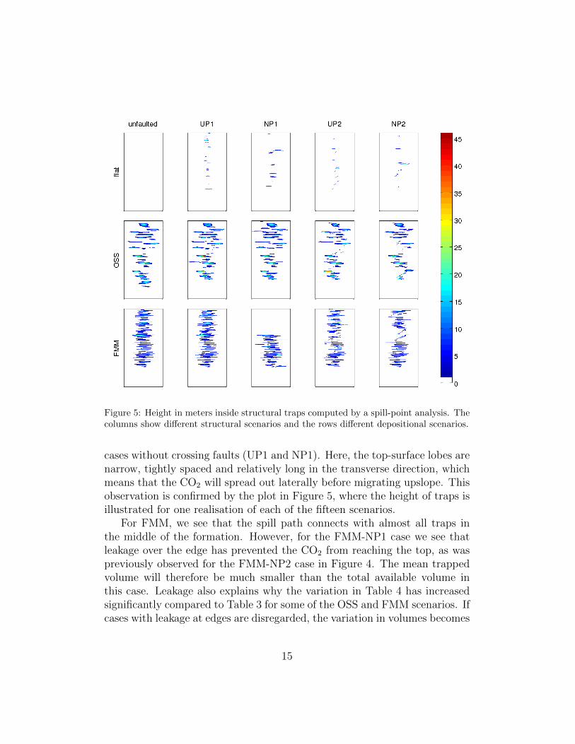
Figure 5: Height in meters inside structural traps computed by a spill-point analysis. Thecolumns show different structural scenarios and the rows different depositional scenarios.
cases without crossing faults (UP1 and NP1). Here, the top-surface lobes arenarrow, tightly spaced and relatively long in the transverse direction, whichmeans that the CO2 will spread out laterally before migrating upslope. Thisobservation is confirmed by the plot in Figure 5, where the height of traps isillustrated for one realisation of each of the fifteen scenarios.
For FMM, we see that the spill path connects with almost all traps inthe middle of the formation. However, for the FMM-NP1 case we see thatleakage over the edge has prevented the CO2 from reaching the top, as waspreviously observed for the FMM-NP2 case in Figure 4. The mean trappedvolume will therefore be much smaller than the total available volume inthis case. Leakage also explains why the variation in Table 4 has increasedsignificantly compared to Table 3 for some of the OSS and FMM scenarios. Ifcases with leakage at edges are disregarded, the variation in volumes becomes
15
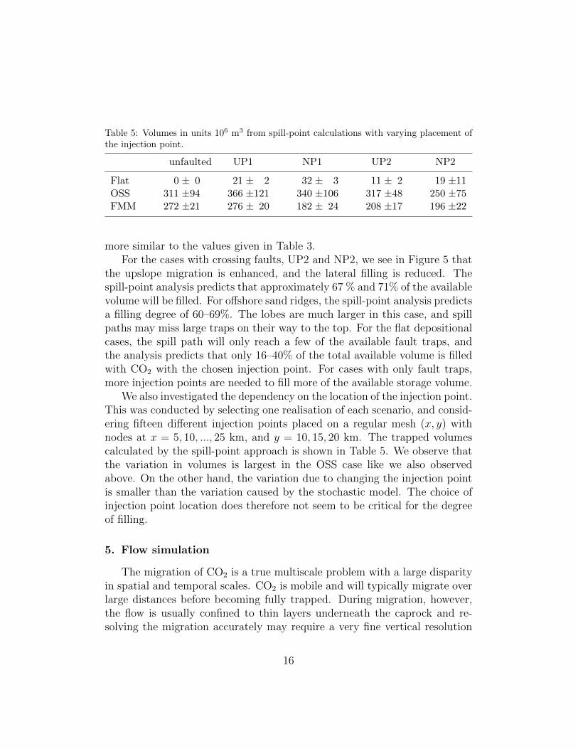
Table 5: Volumes in units 106 m3 from spill-point calculations with varying placement ofthe injection point.
unfaulted UP1 NP1 UP2 NP2
Flat 0 ± 0 21 ± 2 32 ± 3 11 ± 2 19 ±11OSS 311 ±94 366 ±121 340 ±106 317 ±48 250 ±75FMM 272 ±21 276 ± 20 182 ± 24 208 ±17 196 ±22
more similar to the values given in Table 3.For the cases with crossing faults, UP2 and NP2, we see in Figure 5 that
the upslope migration is enhanced, and the lateral filling is reduced. Thespill-point analysis predicts that approximately 67 % and 71% of the availablevolume will be filled. For offshore sand ridges, the spill-point analysis predictsa filling degree of 60–69%. The lobes are much larger in this case, and spillpaths may miss large traps on their way to the top. For the flat depositionalcases, the spill path will only reach a few of the available fault traps, andthe analysis predicts that only 16–40% of the total available volume is filledwith CO2 with the chosen injection point. For cases with only fault traps,more injection points are needed to fill more of the available storage volume.
We also investigated the dependency on the location of the injection point.This was conducted by selecting one realisation of each scenario, and consid-ering fifteen different injection points placed on a regular mesh (x, y) withnodes at x = 5, 10, ..., 25 km, and y = 10, 15, 20 km. The trapped volumescalculated by the spill-point approach is shown in Table 5. We observe thatthe variation in volumes is largest in the OSS case like we also observedabove. On the other hand, the variation due to changing the injection pointis smaller than the variation caused by the stochastic model. The choice ofinjection point location does therefore not seem to be critical for the degreeof filling.
5. Flow simulation
The migration of CO2 is a true multiscale problem with a large disparityin spatial and temporal scales. CO2 is mobile and will typically migrate overlarge distances before becoming fully trapped. During migration, however,the flow is usually confined to thin layers underneath the caprock and re-solving the migration accurately may require a very fine vertical resolution
16
in 3D simulations.Using a vertical equilibrium (VE) assumption (Nordbotten and Celia,
2012), the flow of a thin CO2 plume can be approximated in terms of itsthickness to obtain a 2D simulation model. Although this approach reducesthe dimension of the model, important information of the heterogeneities inthe underlying 3D medium is preserved. In fact, the errors resulting from theVE assumption will in many cases be significantly smaller than the errorsintroduced by the overly coarse resolution needed to make the 3D simulationmodel computationally tractable. In addition, integrating the flow equationsvertically improves the time constants of the model and typically leads to alooser dynamical coupling, e.g., between flow and transport. Vertical equi-librium simulations will therefore in many cases be an attractive method toincrease (lateral) resolution while saving computational cost, in particularfor scenarios similar to those considered herein.
As above, our injection scenario consists of a single well positioned at(15, 15) km, which will inject at a constant rate of ten million cubic me-ters per year for 50 years. In total, we will follow the formation of a CO2
plume and its subsequent upslope migration for a period of 5000 years. Fluidproperties will generally depend on pressure and thus height along the forma-tion. To simplify the flow simulations, we neglect the pressure dependenceand assume all fluids to be incompressible and be described by the followingfluid parameters: CO2 is assumed to be a supercritical fluid with viscosityof 0.057 cP, constant density of 686 kg/m3, and a quadratic relative perme-ability with residual saturation of 0.2 and endpoint scaling factor of 0.2142.For water, we assume a viscosity of 0.31 cP, density of 975 kg/m3, residualsaturation of 0.1, and endpoint scaling of 0.85. During injection we imposehydrostatic boundary conditions, whereas no-flow boundary conditions areassumed during the post-injection period.
5.1. Estimates of trapping
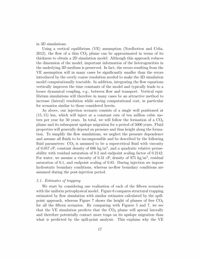
We start by considering one realisation of each of the fifteen scenarioswith the uniform petrophysical model. Figure 6 compares structural trappingestimated by flow simulation with similar estimates calculated by the spill-point approach, whereas Figure 7 shows the height of plumes of free CO2
for all the fifteen scenarios. By comparing with Figures 5 and 7, we seethat the VE simulation predicts that the CO2 plume will spread laterallyand therefore potentially contact more traps on its upslope migration thanwhat is predicted by the spill-point analysis. This explains why the VE
17

simulation predicts larger structural trapped volumes for the flat depositionalscenarios. For the OSS and FMM scenarios, the VE simulation predicts thatthe plume has not reached the top of the structure after 5000 years in mostof realisations. The spill-point calculation, on the other hand, continuesto fill traps until some CO2 reaches the top of the formation, and henceoverestimates the volumes that are structurally trapped after 5000 years.
With flow simulation, we can also find free and residually trapped vol-umes. The free volume is defined as the volume that is not residually trapped,and includes volumes confined in fold and fault traps. Figure 8 gives the freeand residually trapped volumes computed by flow simulation. We observethat the residual trapping is largest for the flat depositional cases, for whichthe plume has reached the top of the structure within 5000 years. In thiscase, there is almost no relief in the top-surface morphology that will retardthe plume migration and hence the plume will sweep a large volume withinthe migration period. For the OSS and FMM scenarios, the plume is retardedby the lobes in the top surface, and residual trapping is reduced comparedwith the surface without reliefs. Eventually, however, the residual trappingwill increase also for these scenarios.
The most striking observation that can be made from Figures 6 to 8is that structure has a limited influence on the free and residual volumescompared with the sedimentary scenarios OSS and FMM. In practise, thismeans that top-surface morphology caused by faulting has less effect thanthe morphology caused by sedimentary architectures. This is an interestingobservation given that modellers tend to put a lot of effort into describingfaults and ignore sedimentary effects on the top-surface morphology. (Onthe other hand, our observation may be biased by the fact that we have usedsimple fault model in which all faults are assumed to be sealing.)
5.2. Effect of high-permeable top
Both beach rides and shelf ridges will often have a higher grain size to-wards the top, which is reflected in a simple way by our second petrophysicalmodel that has a high-permeable top layer.
Figures 9 and 10 report differences in movable and structurally trappedCO2 volumes, respectively, predicted by the two models. A high-permeabletop leads to increased structural trapping in all cases except for OSS-NP2,but has different effects on the movable volume for the three sedimentaryscenarios. Figures 11 and 12 show that for the FMM and the flat deposi-tional scenarios, the plume will move faster to the top, thereby increasing the
18
Unfaulted UP1 NP1 UP2 NP2Flat 0 22 31 11 16OSS 324 370 352 315 250FMM 276 289 183 209 205
0
50
100
150
200
250
300
350
400
Million m3
Spill point
Unfaulted UP1 NP1 UP2 NP2Flat 0 34 20 24 27OSS 150 164 150 158 141FMM 111 101 115 93 95
0
50
100
150
200
250
300
350
400
Million m3
Vertical equilibrium
Figure 6: Comparison of structurally trapped volumes in units of million cubic meterscomputed by spill-point analysis and VE simulation.
19

Figure 7: Height in meters for the plumes of free CO2 after 5000 years. The columns showdifferent structural scenarios and the rows different depositional scenarios.
20

Unfaulted UP1 NP1 UP2 NP2Flat 214 248 248 238 263OSS 355 365 357 357 360FMM 300 304 315 305 305
0
50
100
150
200
250
300
350
400
Million m3
Free volumes
Unfaulted UP1 NP1 UP2 NP2Flat 297 263 263 273 248OSS 156 146 153 154 151FMM 211 207 196 206 206
0
50
100
150
200
250
300
350
400
Million m3
Residually trapped
Figure 8: Free and residually trapped volumes in units of million cubic meters computedby a VE simulation.
21
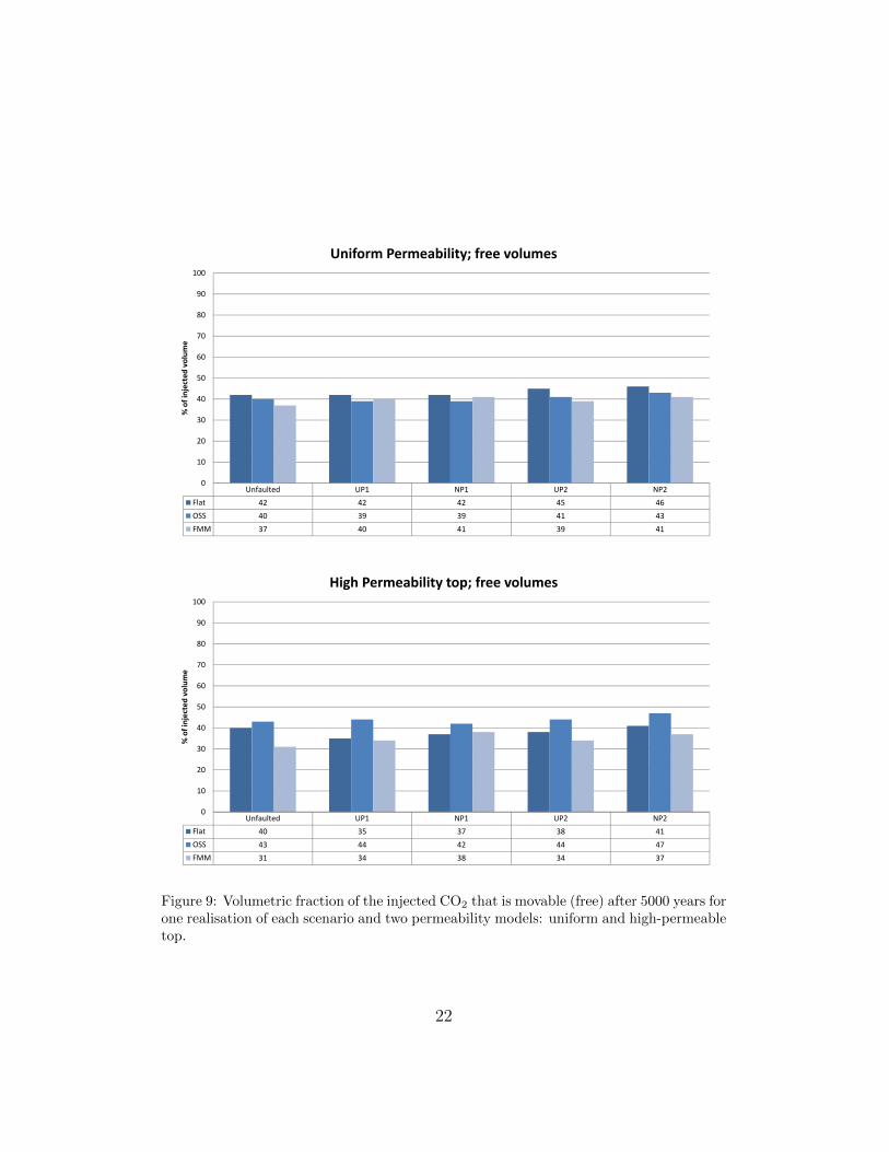
Unfaulted UP1 NP1 UP2 NP2Flat 42 42 42 45 46OSS 40 39 39 41 43FMM 37 40 41 39 41
0
10
20
30
40
50
60
70
80
90
100
% of injected volume
Uniform Permeability; free volumes
Unfaulted UP1 NP1 UP2 NP2Flat 40 35 37 38 41OSS 43 44 42 44 47FMM 31 34 38 34 37
0
10
20
30
40
50
60
70
80
90
100
% of injected volume
High Permeability top; free volumes
Figure 9: Volumetric fraction of the injected CO2 that is movable (free) after 5000 years forone realisation of each scenario and two permeability models: uniform and high-permeabletop.
22

Unfaulted UP1 NP1 UP2 NP2Flat 0 7 5 4 5OSS 29 32 31 29 28FMM 22 20 18 23 19
0
10
20
30
40
50
60
70
80
90
100
% of injected volume
Uniform Permeability; residually trapped volumes
Unfaulted UP1 NP1 UP2 NP2Flat 0 7 5 5 7OSS 30 31 32 29 27FMM 27 25 22 28 23
0
10
20
30
40
50
60
70
80
90
100
% of injected volume
High Permeability top; residually trapped
Figure 10: Volumetric fraction of the injected CO2 that is residually trapped after 5000years for one realisation of each scenario and two permeability models: uniform and high-permeable top.
23

Flat UP2 OSS UP2 FMM UP2
uniform high-perm uniform high-perm uniform high-perm
Figure 11: Height of the CO2 plume after 1425 years (top) and 4525 years (bottom) forstructural model UP2, the three different sedimentary scenarios, and the two petrophysicalmodels.
Figure 12: Maximum upslope position (in kilometres) of the CO2 plume as a functionof time (in years) for the three sedimentary scenarios: flat (solid line), OSS (dotted),and FMM (dash-dot). Blue colour denotes uniform permeability and red denotes high-permeable top layer.
24

residual trapping and decreasing the movable volume. For the OSS scenarios,on the other hand, a high-permeable top will retard he plume migration andthus increase the volume fraction that is movable after 5000 years. Here, theheight of the lobes in the top surface is so large that many spill points willbe located within the low-permeable part of the reservoir.
6. Coarsening the top surface
In the simulations described above, we have used a relatively simple flowmodel that only accounts for incompressible two-phase effects. For such asimple flow model, there are several methods available that enable forwardsimulations to be conducted with high efficiency. Herein, we used verticalintegration of the flow equations that reduced the computational cost of theflow simulation and enabled us to run a single forward simulation at the fullmodel resolution within hours on a powerful workstation. However, even witha sixteen-core shared-memory computer at our disposal, we still found thatrunning fully resolved flow simulations for the whole ensemble of 2×14×100model realisations was computationally intractable within a few days. Onemay, of course, argue that the problem would be computationally tractable ifwe had chosen a more powerful computer or extended our time frame. On theother hand, the computational cost associated with each forward simulationwill increase dramatically once one starts to add more physical effects intothe flow model. In our opinion, some degree of upscaling of our geologicalrepresentation is therefore inevitable to allow us to conduct a full Monte Carlotype uncertainty analysis. To this end, we will consider a simple upscalingin which the grid is coarsened a factor two or a factor four in each lateraldirection so that the new top surface can be obtained by a straightforwardresampling (interpolation).
In the remains of this section, we will investigate to what extent thegrid models can be coarsened without loosing relevant detail. First of all,coarsening the grid may potentially change the top surface and thereby thevolumes available for structural trapping. Figure 13 shows how this will affectour estimates for the volume available to structural trapping. The effect ismost pronounced for the FMM cases, which have the most detailed geometryin the form of small and densely populated lobes that are flattened whenresampled on a coarser grid. Hence, the fine-scale details are not conservedduring coarsening and structurally trapped volumes become too small. TheOSS sedimentary cases, on the other hand, have significantly larger lobes and
25

0 500 1000 1500 2000 2500 3000 3500 40000
500
1000
1500
2000
2500
3000
3500
4000
original
2x2
co
ars
en
ed
flatUP1
flatUP2
flatNP1
flatNP2
OSS
OSSUP1
OSSUP2
OSSNP1
OSSNP2
FMM
FMMUP1
FMMUP2
FMMNP1
FMMNP2
0 500 1000 1500 2000 2500 3000 3500 40000
500
1000
1500
2000
2500
3000
3500
4000
original
4x4
co
ars
en
ed
flatUP1
flatUP2
flatNP1
flatNP2
OSS
OSSUP1
OSSUP2
OSSNP1
OSSNP2
FMM
FMMUP1
FMMUP2
FMMNP1
FMMNP2
Figure 13: Scatter plot of total volume available in structural traps for coarsened surfacesversus the same volume from the original grid for fifteen realisations of each of the fourteenscenarios. To the left, a factor two is used in the coarsening, to the right the coarseningfactor is four.
26
OSS UP2 FMM UP2
original 4× 4 upscaled original 4× 4
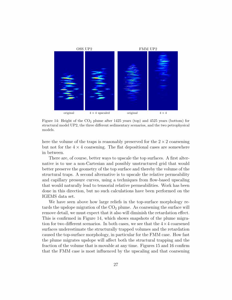
Figure 14: Height of the CO2 plume after 1425 years (top) and 4525 years (bottom) forstructural model UP2, the three different sedimentary scenarios, and the two petrophysicalmodels.
here the volume of the traps is reasonably preserved for the 2× 2 coarseningbut not for the 4 × 4 coarsening. The flat depositional cases are somewherein between.
There are, of course, better ways to upscale the top surfaces. A first alter-native is to use a non-Cartesian and possibly unstructured grid that wouldbetter preserve the geometry of the top surface and thereby the volume of thestructural traps. A second alternative is to upscale the relative permeabilityand capillary pressure curves, using a techniques from flow-based upscalingthat would naturally lead to tensorial relative permeabilities. Work has beendone in this direction, but no such calculations have been performed on theIGEMS data set.
We have seen above how large reliefs in the top-surface morphology re-tards the upslope migration of the CO2 plume. As coarsening the surface willremove detail, we must expect that it also will diminish the retardation effect.This is confirmed in Figure 14, which shows snapshots of the plume migra-tion for two different scenarios. In both cases, we see that the 4×4 coarsenedsurfaces underestimate the structurally trapped volumes and the retardationcaused the top-surface morphology, in particular for the FMM case. How fastthe plume migrates upslope will affect both the structural trapping and thefraction of the volume that is movable at any time. Figures 15 and 16 confirmthat the FMM case is most influenced by the upscaling and that coarsening
27
the surface here will produce a significant, and possibly unacceptable, biasin the estimates. For the OSS and flat depositional scenarios, more reliableestimates can be obtained also from the upscaled models.
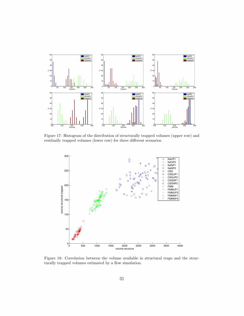
For completeness, we also show how coarsening the top surface affects thedistribution functions that can be derived from the one hundred realisations.Figure 17 shows histograms for structural scenario NP2 with different upscal-ing factors for all three sedimentary scenarios. Here, we clearly observe thatwhereas the distribution functions for the OSS and flat depositional scenariosare only slightly perturbed, the FMM distribution shifts significantly alongthe axis with increasing degree of coarsening.
7. Discussion
In the previous sections we have shown both simplified geometrical anal-ysis of structural trapping (spill point and cascades of traps) as well as es-timates based upon more comprehensive flow simulations. Fast estimationof fluid responses is essential to use a Monte Carlo type approach to studythe influence of geological uncertainty on plume migration and fluid trap-ping. Hence, a key question is: how reliable estimates can we get from thesimplified models?
Figure 18 shows the correlation between the theoretical capacity for struc-tural trapping estimated from the cascade of traps and the structurallytrapped volumes estimated by fluid simulation. For the FMM and flat de-positional scenarios, which both have small-scale reliefs in their morphology,the two estimates correlate well. The OSS scenarios, on the other hand, showmuch larger variation because of the larger lobes and although a geometricalanalysis may give indicative numbers of actual trapping, this type of estimatewill generally be less reliable.
Figure 19 shows a similar correlation plot for residual trapping versusvolumes available. The figure indicates a negative correlation between thetwo, which is somewhat misleading. Instead, the figure shows the correlationbetween structural volume and how much the plume migration is retarded;see the discussion above. After 5000 years, the plume has reached the topand all possible residual trapping has taken place for the flat depositionalscenarios. For the OSS and FMM scenarios, the plume has not yet reachedthe top and further residual trapping is likely to take place at a later time.
28

0 50 100 150 200 250 3000
50
100
150
200
250
300
original
2x2
co
ars
en
ed
flatUP1
flatUP2
flatNP1
flatNP2
OSS
OSSUP1
OSSUP2
OSSNP1
OSSNP2
FMM
FMMUP1
FMMUP2
FMMNP1
FMMNP2
0 50 100 150 200 250 3000
50
100
150
200
250
300
original
4x4
co
ars
en
ed
flatUP1
flatUP2
flatNP1
flatNP2
OSS
OSSUP1
OSSUP2
OSSNP1
OSSNP2
FMM
FMMUP1
FMMUP2
FMMNP1
FMMNP2
Figure 15: Scatter plot of structurally trapped volumes estimated from coarsened surfacesversus the same volumes estimated from the original surface.
29

0 50 100 150 200 250 3000
50
100
150
200
250
300
original
2x2
co
ars
en
ed
flatUP1
flatUP2
flatNP1
flatNP2
OSS
OSSUP1
OSSUP2
OSSNP1
OSSNP2
FMM
FMMUP1
FMMUP2
FMMNP1
FMMNP2
0 50 100 150 200 250 3000
50
100
150
200
250
300
original
4x4
co
ars
en
ed
flatUP1
flatUP2
flatNP1
flatNP2
OSS
OSSUP1
OSSUP2
OSSNP1
OSSNP2
FMM
FMMUP1
FMMUP2
FMMNP1
FMMNP2
Figure 16: Scatter plot of movable volume estimated from coarsened surfaces versus thesame volumes estimated from the original surface.
30
50 100 150 200 250 3000
10
20
30
40
50
60
Volume
%
flatNP2
OSSNP2
FMMNP2
50 100 150 200 250 3000
10
20
30
40
50
60
Volume
%
flatNP2
OSSNP2
FMMNP2
50 100 150 200 250 3000
10
20
30
40
50
60
Volume
%
flatNP2
OSSNP2
FMMNP2
100 150 200 250 3000
10
20
30
40
50
60
Volume
%
flatNP2
OSSNP2
FMMNP2
100 150 200 250 3000
10
20
30
40
50
60
Volume
%
flatNP2
OSSNP2
FMMNP2
100 150 200 250 3000
10
20
30
40
50
60
Volume
%
flatNP2
OSSNP2
FMMNP2
Figure 17: Histogram of the distribution of structurally trapped volumes (upper row) andresidually trapped volumes (lower row) for three different scenarios.
0 500 1000 1500 2000 2500 3000 3500 40000
50
100
150
200
250
300
volume structure
volu
me s
tructu
ral tr
apped
flatUP1
flatUP2
flatNP1
flatNP2
OSS
OSSUP1
OSSUP2
OSSNP1
OSSNP2
FMM
FMMUP1
FMMUP2
FMMNP1
FMMNP2
Figure 18: Correlation between the volume available in structural traps and the struc-turally trapped volumes estimated by a flow simulation.
31

0 500 1000 1500 2000 2500 3000 3500 4000100
120
140
160
180
200
220
240
260
280
300
volume structure
resid
ual tr
apped
flatUP1
flatUP2
flatNP1
flatNP2
OSS
OSSUP1
OSSUP2
OSSNP1
OSSNP2
FMM
FMMUP1
FMMUP2
FMMNP1
FMMNP2
Figure 19: Correlation between the volume available in structural traps and the residuallytrapped volumes estimated by a flow simulation.
32

8. Conclusion
Trapping of CO2 is significantly affected by top-surface morphology, whichcontributes both to structural trapping and retardation of the plume migra-tion. As a result, the statistics of the top-surface morphology has a stronginfluence on the statistics of the trapped fluid. However, the spread of theplume is only inhibited if the height of the plume is of the same scale as theamplitude of the relief. A modest relief may therefore retard the migrationfor low injection rates, but have negligible effect for high injection rates thatcreate a thick plume.
For the specific parameters considered herein, structural and residualtrapping are equally important. More surprising, we observe that fault-ing has less influence on the free and residual volumes than the top-surfacemorphology induced by sedimentary architecture, which is often neglectedin geological modelling. Our observation may be an effect of overly simpli-fied model choices, but should nevertheless be more thoroughly investigatedbecause of its potential implications of how large-scale aquifers should bemodelled.
The interplay between structural and residual trapping is generally non-trivial. Still, our analysis shows that the potential for structural trapping canbe efficiently estimated for large model ensembles using simplified modelling:Cascades of structural traps are effectively identified by a simple geomet-rical analysis and can be used to bound the structural trapping capacity.Likewise, rough estimates for actual trapping from specific injection pointscan be efficiently calculated using a spill-point analysis. Residual trapping,on the other hand, appears to be less correlated with simple volume esti-mates and must generally be resolved by detailed flow simulations. To thisend, models based upon vertical integration have proved very useful becauseof significantly reduced computational cost and improved vertical resolutioncompared with traditional 3D modelling.
The need for further upscaling, and the effect that such an upscaling hason flow predictions, will depend highly on the sedimentary and structuralscenarios. Our scenarios with buried offshore sand ridges (OSS) have largelobes and are not strongly affected by (modest) coarsening of the top surface.The flooded marginal-marine (FMM) scenarios, on the other hand, consistof dense patterns of small-scale structures that are quite sensitive to gridresolution and cannot be coarsened geometrically in a straightforward waywithout loosing essential detail. One alternative is to use a more elaborate
33

flow-based upscaling, but this may lead to complicated models with tensorialrelative permeabilities.
Altogether, our analysis demonstrates that uncertainty in morphologyeffects at a small scale may have a significant impact on estimates of struc-tural and residual trapping. A future research direction would therefore beto develop a more truly multiscale framework that can properly account forsmall-scale effect when simulating large-scale CO2 plume migration.
9. Acknowledgements
This work was supported by the Norwegian Research Council throughgrant no. 200026 from the CLIMIT programme.
References
Ashraf, M., Lie, K.-A., Nilsen, H. M., Skorstad, A., 2010. Impact of geologicalheterogeneity on early-stage CO2 plume migration: sensitivity study. In:Proceedings of the 12th European Conference on the Mathematics of OilRecovery (ECMOR XII), Oxford, UK, 6–9 September 2010. EAGE.
Celia, M. A., Nordbotten, J. M., Bachu, S., Kavetski, D., Gasda, S.,2010. Summary of princeton workshop on geological storage of CO2.Princeton-bergen series on carbon storage, Princeton University, uri:http://arks.princeton.edu/ark:/88435/dsp01jw827b657.
Chadwick, A., Williams, G., Delepine, N., Clochard, V., Labat, K., Sturton,S., Buddensiek, M., Dillen, M., Nickel, M., Lima, A., Arts, R., Neele,F., Rossi, G., 2010. Quantitative analysis of time-lapse seismic monitoringdata at the Sleipner CO2 storage operation. The Leading Edge, 170–177.
Chadwick, R. A., Noy, D. J., 2010. History-matching flow simulations andtime-lapse seismic data from the Sleipner CO2 plume. In: PetroleumGeology: From Mature Basins to New Frontiers Proceedings of the 7thPetroleum Geology Conference. Vol. 7 of Petroleum Geology Conferenceseries. Geological Society, London, pp. 1171–1182.
Class, H., Ebigbo, A., Helmig, R., Dahle, H. K., Nordbotten, J. M., Celia,M. A., Audigane, P., Darcis, M., Ennis-King, J., Fan, Y., Flemisch, B.,Gasda, S. E., Jin, M., Krug, S., Labregere, D., Beni, A. N., Pawar, R. J.,
34
Sbai, A., Thomas, S. G., Trenty, L., Wei, L., 2009. A benchmark study onproblems related to CO2 storage in geologic formations. Comput. Geosci.13 (4), 409–434.
Curray, J. R., Moore, D. G., 1964. Holocene regressive littoral sand, Costa deNayarit, Mexico. In: Van Straaten, L. M. J. U. (Ed.), Deltaic and ShallowMarine Deposits. Elsevier, pp. 76–82.
Dyer, K. R., Huntley, D. A., 1999. The origin, classification and modellingof sand banks and ridges. Continental Shelf Research 19, 1285–1330.
Eiken, O., Ringrose, P., Hermanrud, C., Nazarian, B., Torp, T., Hier, L.,2011. Lessons learned from 14 years of ccs operations: Sleipner, In Salahand Snøhvit. Energy Procedia 4, 5541–5548.
Hollund, K., Mostad, P., Nielsen, B. F., Holden, L., Gjerde, J., Contursi,M. G., McCann, A. J., Townsend, C., Sverdrup, E., 2002. Havana — a faultmodeling tool. In: Koestler, A. G., Hunsdale, R. (Eds.), Hydrocarbon SealQuantification. Norwegian Petroleum Society Conference, 16–18 October2002, Stavanger, Norway. Vol. 11 of NPF Special Publication. Elsevier.
Houthuys, R., Gullentops, F., 1988. The Vlierzele Sands (Eocene, Belgium):a tidal ridge system. In: Tide-influenced sedimentary environments andfacies. D. Reidel Publishing Co., Dordrecht, pp. 139–152.
IGEMS, 2011. Impact of realistic geologic models on simulation of co2 storage(igems). http://igems.nr.no.
Jackson, C. A.-L., Grunhagen, H., Howell, J. A., Larsen, A. L., Andersson,A., Boen, F., Groth, A., 2010. 3D seismic imaging of lower delta-plainbeach ridges: lower Brent Group, northern North Sea. Journal of the Ge-ological Society of London 167, 1225–1236.
Manzocchi, T., et al., 2008. Sensitivity of the impact of geological uncertaintyon production from faulted and unfaulted shallow-marine oil reservoirs:objectives and methods. Petrol. Geosci. 14 (1), 3–15.
Nielsen, L. H., Johannessen, P. N., 2001. Accretionary, forced regressiveshoreface sands of the Holocene-recent Skagen Odde spit complex, Den-mark – a possible outcrop analogue to fault-attached shoreface sandstone
35

reservoirs. In: Martinsen, O. J., Dreyer, T. (Eds.), Sedimentary Envi-ronments Offshore NorwayPalaeozoic to Recent. Vol. 10 of NPF specialpublication. Norsk petroleumsforening, Elsevier, pp. 457–472.
Nordbotten, J. M., Celia, M. A., 2012. Geological Storage of CO2: ModelingApproaches for Large-Scale Simulation. John Wiley & Sons.
Nummedal, D., Riley, G. W., 1999. The origin of the Tocito Sandstone and itssequence stratigraphic lessons. In: Isolated Shallow Marine Sand Bodies:Sequence Stratigraphic Analysis and Sedimentologic Interpretation. Vol. 64of SEPM Special Publication. Bergman, K. M. and Snedden, J. W., pp.227–254.
Nummedal, D., Suter, J., 2002. Continental shelf sand ridges; genesis, stratig-raphy and petroleum significance. In: 22nd Annual Gulf Coast SectionSEPM Foundation Bob F. Perkins Research Conference Proceedings. pp.503–518.
Otvos, E. G., 2000. Beach ridges definition and significance. Geomorphology32, 83–108.
Posamentier, H. W., 2002. Ancient shelf ridges-a potentially significant com-ponent of the transgressive systems tract: case study from offshore north-west java. AAPG Bullentine 86, 75–106.
Pruess, K., Garca, J., Kovscek, T., Oldenburg, C., Rutqvist, J., Steefel,C., Xu, T., 2004. Code intercomparison builds confidence in numericalsimulation models for geologic disposal of CO2. Energy 29 (9–10), 1431–1444.
Riley, G. W., 1993. Origin of a coarse-grained shallow marine sandstone com-plex: the Coniacian Tocito Sandstone, northwestern New Mexico. Ph.D.thesis, Louisiana State University.
Stapor, F. W. J., Matthews, T. D., Lindfors-Kearns, F. E., 1991. Barrier-island progradation and Holocene sea-level history in southwest Florida.Journal of Costal Research 7, 815–838.
Suter, J. R., Clifton, H. E., 1999. The Shannon Sandstone and isolated lin-ear sand bodies: interpretations and realizations. In: Isolated ShallowMarine Sand Bodies: Sequence Stratigraphic Analysis and Sedimentologic
36

Interpretation. Vol. 64 of SEPM Special Publication. Bergman, K. M. andSnedden, J. W., pp. 321–356.
Torabi, A., Berg, S. S., 2011. Scaling of fault attributes: A review. Marineand Petroleum Geology 28, 1440–1460.
37