Journal of Business Studies Quarterly

December 2016, Volume 8, Number 2 ISSN 2152-1034

Impact of Remittances and FDI on Economic Growth: A Panel Data

Analysis

Dr. Jannatul Ferdaous Assistant Professor

Department of Finance and Banking, Faculty of Business Studies,

Bangladesh University of Professionals, Mirpur Cantonment,

Dhaka, Bangladesh.Email:jannat.du@hotmail.com

Abstract:

International capital flows have generally been considered crucial for economic growth. This

study makes an empirical contribution to explore the impact of Remittances and FDI on the

economic growth of selected developing countries. A panel dataset of 33 developing countries

observed from 2003 to 2014 are examined to explore the impact of both Remittances and FDI on

economic growth. The study apply both static and dynamic panel data approach. In both dynamic

and static framework, the study has found a positive and statistically significant impact of FDI on

the economic growth for the developing countries in sample. The result suggests that FDI has the

potential of improving economic growth for the developing countries in sample. After controlling

for potential endogeneity bias the study reveals that remittance has significant negative impact on

the economic growth across the developing countries in sample over the study period. The result

indicates that most remittance receipts are not channeled to productive uses and the motive of

remitting to the home country economies is mostly altruistic rather than profit driven. The full

benefit of Remittances can be gained by formulation of policy measures to channel Remittances

into some economically productive uses.

Key Words: Economic Growth, Remittances, FDI, Panel Data, Generalized Method of Moments

(GMM).

1.0 Introduction

In the past twenty five years a significant restructuring of international capital flows is observed

to many developing countries, especially through the stimulation of foreign direct investment

(FDI) and the increasing importance of remittances. Simultaneously, other components of

international capital flow; such as international aid, portfolio equity investment, and portfolio debt

investment have decreased and become less influential. These capital flows from rich to poor

countries are very motivating because they can finance investment and consumption, helping

improve the standard of living, stimulating economic growth, and potentially increasing welfare

59

in the developing world. In addition, as a key aspect in economic growth depends in the possession

of physical and financial assets to incorporate advance technologies and create wealth, the

dependence of foreign capital helps fill the gap between savings and investment in capital- scarce

economies. These international capital inflows are also believed to encourage technological

upgrade and financial transformation, and contribute to the growth and productivity of countries

with enough human capital and infrastructure. They are mainly important for the developing

economies for their technological lag and low levels of domestic savings, which has encouraged

local governments to engage in bold policies to make up for their lack of capital.

1.1 Rationale of the Study

Existing empirical literatures in the association between international capital flows and economic

growth is deficient and inconclusive in fundamental ways. Most of the empirical studies are mainly

focused on the contribution of FDI on economic growth .The studies that aim to explore the

contribution of FDI on economic growth have inconclusive results. On the other hand, the

literatures on the Remittances and growth connection are relatively few and the impact of

Remittances on economic growth is still a matter of debate. So, the main contribution of this thesis

is to analyze the effects of both Remittances and FDI on economic growth of selected developing

countries.

1.2 Objective of the Study

There is a vast number of studies about the determinants of FDI and Remittances, however, there

is still a research gap dealing with the impact of Remittances and FDI on economic growth in

developing countries. It is very important to investigate the impact of Remittances and FDI on

economic growth due to their divergent behavior. This study is an endeavor to contribute to the

debate of mixed impact of FDI and Remittances on economic growth. The main objective of this

study is -

To assess whether both Remittances and FDI can significantly promote the economic

growth in developing countries.

In order to achieve the main objective, the specific objectives are-

• To analyze the effect of Remittances on the economic growth of the developing countries.

• To analyze the effect of foreign direct investment (FDI) on the economic growth of the

developing countries.

• To empirically examine the effect of both Remittances and FDI on the economic growth

of the developing countries.

2.0 Review of the Literature

The impact of Remittances on economic growth is still a matter of debate. Remittances are used

for consumption or for investment, sometimes for both. According to some literatures using

Remittances for consumption does not make any good contribution to economic growth. Another

strand of literature argues that Remittances can affect growth by easing liquidity constraints

Remittances can contribute to investment in human and physical capital.

60

Again, there are some studies those find significant negative impacts of Remittances on economic

growth (Chami, Fullenkamp and Jahjah, 2003), or a negative but insignificant impact

(International Monetary Fund [IMF], 2005). On the other hand, remittance can finance education

and health (human capital development) and/or productive investments which bring positive

impact on economic growth. Some of the empirical studies that find Remittances positive effect

on growth are Acosta, Calderón, Fajnzylber and Lopez (2007); Catrinescu, Leon-Ledesma, Piracha

and Quillin (2009); and Guiliano and Ruiz-Arranz (2009).

Researchers who claim that Remittances do not have positive macroeconomic effects have some

major reasons. Firstly, it is believed that Remittances may cause a situation similar to the “Dutch

disease.Secondly, Chami, Fullenkamp and Jahjahha (2005) opine that the Remittances would

create a moral hazard, and lessen the incentive to work. Consequently the productivity of the

country would be reduced, giving negative effect in developing growth. Bettini and Zazzaro (2008)

considers that partial reason why Remittances have not inspired economic growth is that they are

generally not aimed to serve as investments but rather as social insurance to help family members

finance the purchase of life’s necessities. As mentioned earlier most of the Remittances are not

used for investment. Researchers think about a possibility that if the Remittances be used only for

consumption rather than investment, growth would not be gained. Contrary to the conclusion of

Chami, Fullenkamp and Jahjahha(2005), Mansoor and Quillin (2006) have stated that the

Remittances seem to have a positive and statistically significant impact on growth. In their paper,

they addressed the model developed by Chami, Fullenkamp and Jahjahha (2005) was faulty. Based

on their model, some improvements were made like adding institutional variables which were

considered important. These modifications have led to a conclusion with completely opposite

result. Besides, it has emphasized that Remittances would bring positive impact on economic

growth whether through increased consumption, savings, or investment.

Theoretically numerous studies are there which observe the impact of foreign direct investment on

economic growth of the host country. Particularly for developing countries FDI is an important

vehicle for transferring technology, knowledge, forming domestic capital, and opening to global

market. While there are many intuitive reasons to believe FDI’s positive economic growth impact

on the host countries, especially in developing countries where FDI is an engine of growth, the

empirical evidence is mixed. Some studies find negligible effects of FDI on growth ((Akinlo,

2004) ,(Aynwale, 2007) and (Hermes and Lensink ,2003)). Hermes and Lensink (2003) concluded

that FDI applies high negative effect on the host country. According to their studies FDI may cause

crowding out effect on domestic investment, destructive competition of foreign affiliates with

domestic firms, external vulnerability and dependence and “market-stealing effect” as a result of

poor absorptive capacity. Mottaleb (2007) studied the determinants of FDI and its impact on

economic growth in developing countries. He found that FDI has an important effect on economic

growth of third world countries by linking up domestic savings and investment and familiarizing

the latest technology and management skill from developed countries. Lee, Baimukhamedova and

Akhmetova (2009) have found a minimum significant impact of FDI on GDP growth of

Kazakhstan. They analyzed the correlation between FDI inflows, exchange rate, and economic

growth of Kazakhstan by a multivariate regression model with weighted least squares estimates.

Piotr Misztal (2010) researched the influence of FDI on the economic growth in the Romania

during the past decade 2000-2009 using the Vector Autoregression Model (VAR) and found that

the relationship between FDI and economic growth is linear. The literature on FDI and growth

include findings about the effects on growth of interactions of human capital and FDI which are

61

interesting. In this strand of literature, human capital affects the absorptive capacity of the economy

and conditions the positive effects of FDI on economic growth (Borensztein et al., 1998).

Borensztein et al. (1998) highlight the introduction of more advanced technologies through FDI

and examine the effect of the interaction between human capital and FDI on growth. They indentify

that there is a strong complementary effect between human capital and FDI on growth. It is also

revealed that to exert a positive effect of FDI on growth a minimum threshold of human capital is

needed. Thomas, et al. (2008) has argued that investment of Multinational Enterprises (MNE) in

the host country imposes the pressure on the local firms to develop new technologies and innovate.

This also explains the possible reason the developing countries are interested in taking measures

that attract foreign direct investment.

3.0 Empirical Analysis

The aim of this research is to empirically analyze how Remittances and FDI affect economic

growth of developing countries. Most of the studies that have been undertaken before have had

problems with estimations techniques. Easterly, Levine, and Roodman (2004) point out that there

tends to be traps of choosing variables that lack theoretical backing, consequently, researchers

wrongly specify models and get misleading results. Given these reservation, choosing a set of

uncontroversial to estimate the growth effects of FDI and remittances is difficult task. Therefore,

I choose a set of control variables that has been widely used and acknowledged in the empirical

growth literatures and suggested by the standard neoclassical growth model. According to Temple

(1999), the problem that is frequently faced in cross-county growth study is the endogeneity

between growth and the sources of growth; in this case the international private capital flows into

a country. So, I go further to use Generalized Method of Moments (GMM) to deal with the

endogeniety problem.

3.1 Data Description and Data Source

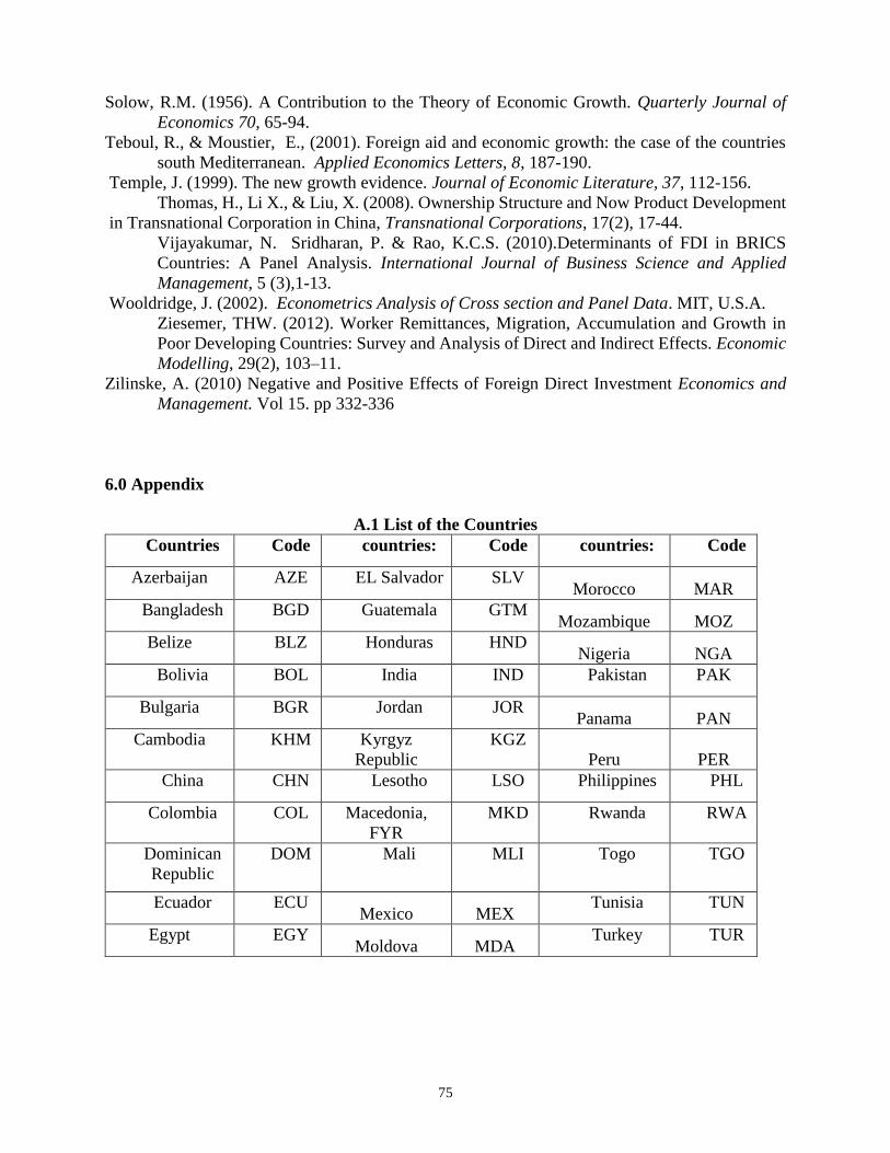
This research is based on the 33 developing countries over the period 2003 to 2014. List of the

countries in the sample is mentioned in the Appendix- A.1. Since I want to look at the effect of

Remittances and FDI on economic growth of developing countries, the countries which have

availability of Remittances and FDI data are sampled. The data which lacks other variables were

excluded. At the end, the data which cannot be logarithmically transformed are eliminated. Among

all developing countries, I used only 33 of them to conduct the econometric analysis. For most

countries the World Bank database included data for the period up to 2014 at the time when I

accessed it. But for a few countries data for some years was missing. In order to fill these gaps, I

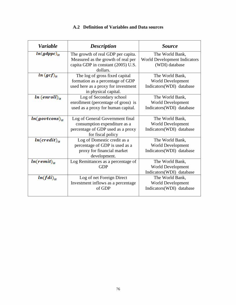
used some other data sources. List of the variables in this study and their data sources is mentioned

in the Appendix- A.2.

3.2 Econometric Model Specification

To determine the responsiveness of Remittances and foreign direct investment (FDI) with the other

traditional the sources of economic growth, I first specify a simple double log-linear Cobb-

Douglass production function as:

62

---------------- (1)

Where, Subscripts i denotes developing countries in sample and subscript t denotes times. The

dependent variable represents the growth of real GDP per capita of country i in year

t. [ ] represents the natural logarithm of Gross fixed capital formation as a share of GDP

which is used as a proxy for physical capital investment. Human capital is represented by

). Secondary school enrollment ratio is used as a proxy for human capital. Based

on the standard growth literatures, other control variables included in this study are-

is Government final consumption expenditure as a percentage of GDP used as

a proxy for fiscal policy. represents financial sector development. Domestic credit

to private sector as a percentage of GDP is used as a proxy for financial market development. The

core variables of interest in this study are which represents Remittances as a

percentage of GDP and is net Foreign Direct Investment (FDI) inflows as a percentage

of GDP. is the disturbance term.

Initially, it is important to mention that macro-econometric modeling is an endeavor to explain the

empirical behavior of an actual economic system. The study used a panel data analysis .There are

several advantages of using panel data sets in econometric research unlike the other data sets. By

using panel data sets, one can easily control for individual unobserved heterogeneity, obtain more

accurate results because it provides more observations and information to work with, it allows

following up individual dynamics and therefore before and after effects can easily be estimated

like in this study ( Temple (2010), Woodridge (2009) and Hsiao (2003)). The above model can be

simplified as follows –

3.2.1 Static Model

The specification of growth equation is based on the static framework of economic growth

model .The general form of the regression equation is given below-

------------------------------- (2)

= Natural logarithm of Real GDP per capita

=Country specific, time invariant effect

=Time specific, country invariant effect

=The vector of the explanatory variables (Gross fixed capital formation as a share of GDP,

School enrollment ratio, Government final consumption expenditure as share of GDP, Domestic

credit to private sector as a share of GDP, Remittance as share of GDP and FDI as a share of GDP)

Subscript (i) = countries (i=1, 2, ….N)

(t) =time (t=1, 2, …T)

= Scalar vector of coefficients of , …

=Error term with E ( ) = 0 and var ( ) = .

)

63

Assumptions for Static Model:

Generally, we can estimate an equation in three different methods, such as- Pooled Ordinary Least

Square (OLS), Fixed Effects (FE) Model and Random Effects (RE) model.

Pooled Ordinary Least Square (OLS):

If country specific effects are constant over time and there is no time specific effect then

we can apply Pooled Ordinary least squares (OLS) method. There may be omitted variable bias

when working with Pooled Ordinary least squares (OLS) estimators. Omitted variables may be

due to data limitation or ignorance. In a panel data model, the omitted variable bias resulting from

the unobserved variable in the error term that is possibly correlated with one or more of the

explanatory variables is also referred to as “unobserved heterogeneity”. This unobserved

heterogeneity can be handled with three possible ways, Such as - One way is to disregard the

problem and get biased and inconsistent estimators. The second approach is to try to find a proxy

variable for the unobserved variable but they are likely to be measured with errors. Alternatively,

we could assume that the omitted variable is constant over time and use certain statistical methods

to control for the unobserved heterogeneity.

Fixed Effects Model:

The unobserved heterogeneity of the developing countries may lead to country-specific

unobserved characteristics be correlated with the explanatory variables in the model. One of the

possible options for handling the unobserved heterogeneity is to use Fixed Effects (FE) to control

for the unobserved effects. So, the second method of the regression equation assumes constant but

not homogenous country specific effects, which leads to Fixed Effects (FE) model. “Fixed Effects

(FE) model is the best fit if we assume that the unobserved heterogeneity among the countries only

results in parametric shifts of the regression function and that it is correlated with one or more of

the explanatory variables (Wooldridge, 2002)”.

Random Effects (RE) Model:

Random Effects (RE) model is the third method of the regression analysis. In case of Random

Effect model we assume non-constant country specific effects and the time effects are absent. In

case of Random Effects model we can control for the unobservable heterogeneity through a general

least-square estimation (GLS) process if it is assumed that the error terms of each individual

countries are randomly distributed across countries and hence the unobserved effects is

uncorrelated with any explanatory variables .

Fixed Effects (FE) is generally regarded as a better tool to control for the unobserved heterogeneity

for estimation since it allows correlation between the unobserved effects and the explanatory

variables. In this research, I have particularly; found it very difficult to collect data for the measures

of some political and institutional variables for the developing countries. It is reasonable to believe

that those political and institutional variables are correlated with some of the explanatory variables.

Therefore, it is not easy to theoretically justify the assumption of the Random Effects (RE) model

that the unobserved effects of the individual developing country are uncorrelated with one or more

of the explanatory variables.

64

In this study, I have used data from 33 developing countries over a twelve-year period. Such

aggregate geographical units cannot be treated as a random sample from a large population. Fixed

Effects (FE) model seems always a more reliable choice than Random Effects model to control for

the unobserved heterogeneity when aggregate data is used.

A formal statistical test can guide the choice between Fixed Effects (FE) model and Random

Effects (RE) model. Hausman (1978) proposed a specification test; “Under the null hypothesis of

no misspecification, there exists a consistent, asymptotically normal and asymptotically efficient

estimator. Under the alternative hypothesis of misspecification, however, this estimator will be

biased and inconsistent.” In other words, if there is no misspecification that means if the individual

effects are uncorrelated with one or more of the explanatory variables, both Fixed Effects (FE) and

Random Effects (RE) estimators are consistent and it does not matter which one is used, or the

sampling variation in the Fixed Effects (FE) is too large to conclude whether the difference is

statistically significant. Hence the likelihood of making a mistake is minimized by using Random

Effects (RE) estimator. However, if the individual effects are correlated with one or more of the

explanatory variables (misspecification), the assumption of the Random Effects (RE) estimators is

false and Fixed Effects (FE) estimators should be used. Therefore, a rejection of the null hypothesis

of Hausman (1978) specification test implies that the individual effects are correlated with the

explanatory variables and Fixed Effects (FE) estimates should be used.

3.2.2 Dynamic Model

In this study, one of the potential problems concerned with estimation of the impact of Remittances

and FDI on economic growth is endogeneity. It is common in the economic growth regression that

some of the explanatory variables are endogenous. Endogeneity may bias estimates of how the

independent variables in equation affect the dependent variable in model. There are two major

sources of endogeneity such as- ‘Unobservable heterogeneity’ and ‘Simultaneity’. To eliminate

the unobservable heterogeneity, conventionally Fixed Effects estimations are used. However, this

estimation is consistent only when we assume that country characteristics or structures are strictly

exogenous. That is, they are purely random observations through time and are unrelated to the

country’s history. But this assumption is unlikely to be valid in reality. So, while OLS estimation

may be biased due to the fact that it ignores unobservable heterogeneity, fixed-effects estimation

may be biased since it neglects endogeneity.

The problem of endogeneity can be resolved by choosing GMM estimator to estimate the impacts

of FDI and remittance on economic growth in dynamic panel data model framework. The

advantage of this methodology is that it eliminates any bias that may arise from ignoring

endogeneity along with providing theoretically based and powerful instruments that accounts for

simultaneity while eliminating any unobservable heterogeneity. It is best to use dynamic panel

estimation in situations when there are some unobservable factors that affect both the dependent

variable and the explanatory variables, and some explanatory variables are strongly related to past

values of the dependent variable. This is likely to be the case in regressions of impact Remittances

and FDI flows on economic growth. These identified complications are addressed by using the

Arellano and Bond (1991) generalized method of moments (GMM) estimator. Arellano and Bond

(1991) GMM estimator is usually called standard first-differenced GMM estimator. Also, the

augmented version of GMM is proposed by Arellano and Bover (1995) and Blundell and Bond

(1998), which is known as system GMM estimator.

65

To specify the dynamic GMM model, equation (1) can be written as follows-

------------ (3)

where,

= Log of real GDP per capita

= Log of GDP per capita lagged one year

= Set of explanatory variables

= Unobserved country-specific effects

, = Coefficients of parameters to be estimated

= The time-varying error term

Subscript (i) = countries (i=1, 2, ….N)

(t) =time (t=1, 2, …T)

To eliminate unobserved heterogeneity ( Arellano and Bond (1991) suggest first-differencing

Equation (3). By first differencing equation (3) can be written as -

------------------ (4)

The equation can be rewritten as following-

------------------------------- (5)

The equation (5) is known as difference GMM. By differencing the equation, difference GMM

eliminates the unobserved country-specific effect since the disturbance does not vary with time

. Thus eliminating omitted variable bias. Moreover, difference GMM helps

overcome endogeneity by using lagged-values of the explanatory variables as instruments.

However, first-differencing generates a new statistical issue that the constructed differenced error

term ( ) is now correlated with the differenced lagged variable. As a solution, Arellano and

Bover (1995) and Blundell and Bond (1998) propose system GMM. The Arellano-Bover (1995)

and Blundell-Bond (1998) estimator augments Arellano-Bond (1991). It builds a system of two

equations: one is the original equation in levels and the other is the transformed one in differences.

This is known as system GMM. This allows the introduction of more instruments and can improve

efficiency. Instruments for the differenced equation are obtained from the lagged levels of the

explanatory variables, while instruments for the level equation are the lagged differences of

explanatory variables.The consistency of the GMM estimator depends on the validity of the

moment conditions, which can be tested using two specifications tests.

The first test is the Arellano-Bond test for autocorrelation which tests if there is no second

order correlation in disturbances.

The second test, namely the Hansen (1982) J-test of over-identifying restrictions, tests the

validity of the instruments. The ‘joint null hypothesis’ of the Hansen test is that the

instruments are exogenous, i.e. they are not correlated with the error term, and the excluded

instruments are correctly excluded from the estimated equation.(Roodman, 2009).

66

4.0 Empirical Results and Findings

4.1 Results of Static Model

The static model (equation 2) is tested by numerous panel data estimations in order to achieve a

model which yields robust results and best fit data. The panel data regression is run for Pooled

ordinary least square (OLS), Random Effects (RE) and Fixed Effects (FE) models.

In the first instance, I estimated the parameters of equation (2) by the Pooled ordinary least square

(OLS) assuming that country specific effects are constant across countries and there is no time

specific effect. As a second step in the static model, I obtained the parameter estimates of equation

(2) using the Random Effects (RE) with the assumption that the country specific effects are

uncorrelated with the regressors in equation (2). Evidently, it is not settled that the covariates are

uncorrelated with . Therefore, I also ran the Fixed Effects (FE) model which allows for such

correlations. As a common test in panel data estimation, I used the Breuch-Pagan LM test and the

Hausman (1978) specification tests to discriminate among these three estimators. Breuch-Pagan

LM test helps to compare Random Effects (RE) with Pooled ordinary least square (OLS). The null

hypothesis of Breuch-Pagan LM test is that there is no significant difference across countries. In

this study, the null hypothesis is rejected at P < .05 and concludes that there is panel effect and

move to Random Effects (RE) is appropriate. The calculated value of Breuch-Pagan LM test is

presented in Appendix-B: 1. At the third step, I obtained the parameter estimates of equation (2)

using the Fixed Effects (FE) model.

Using Hausman (1978) specification test, I checked the suitability of using a Random Effects (RE)

model over a Fixed Effects (FE) model. The hypothesis for Hausman specification test is –

Hausman(1978) Specification test rejects the null that both Random Effects (RE) and Fixed

Effects (FE) are consistent at p value < 0.05. The result of the Hausman test confirms that the

Fixed Effects (FE) model is superior to Random Effects (RE) model for this study.The following

Table 4.1 reports the estimation results for Pooled OLS estimation, Fixed Effects (FE) model and

Random Effects (RE) model. The column (1) represents the Pooled OLS estimation, column (2)

represents Fixed Effects estimation and column (3) represents Random Effects estimation results.

The discussions of the results are based on the findings of Fixed Effects model which is reported

in column (2) of table 4.3. The results disclose the expected relationship between the economic

growth (Real GDP Per Capita Growth) and the sources of growth (explanatory variables). The

coefficients of the variables represent elasticities because the dependent variable and independent

variables are taken in logs. The shows that the Fixed Effects (FE) model explains 79.6 percent

of the variation in the dependent variable (Real GDP per capita growth). The following table

summarizes the results.

67

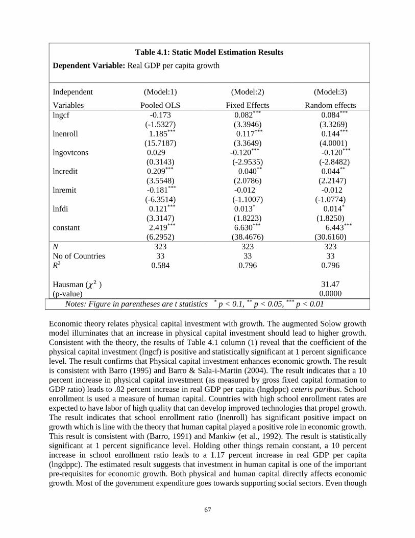
Table 4.1: Static Model Estimation Results

Dependent Variable: Real GDP per capita growth

Independent (Model:1) (Model:2) (Model:3)

Variables Pooled OLS Fixed Effects Random effects

lngcf -0.173 0.082*** 0.084***

(-1.5327) (3.3946) (3.3269)

lnenroll 1.185*** 0.117*** 0.144***

(15.7187) (3.3649) (4.0001)

lngovtcons 0.029 -0.120*** -0.120***

(0.3143) (-2.9535) (-2.8482)

lncredit 0.209*** 0.040** 0.044**

(3.5548) (2.0786) (2.2147)

lnremit -0.181*** -0.012 -0.012

(-6.3514) (-1.1007) (-1.0774)

lnfdi 0.121*** 0.013* 0.014*

(3.3147) (1.8223) (1.8250)

constant 2.419*** 6.630*** 6.443***

(6.2952) (38.4676) (30.6160)

N 323 323 323

No of Countries

R2

33

0.584

33

0.796

33

0.796

Hausman (𝜒2 )

(p-value)

31.47

0.0000

Notes: Figure in parentheses are t statistics * p < 0.1, ** p < 0.05, *** p < 0.01

Economic theory relates physical capital investment with growth. The augmented Solow growth

model illuminates that an increase in physical capital investment should lead to higher growth.

Consistent with the theory, the results of Table 4.1 column (1) reveal that the coefficient of the

physical capital investment (lngcf) is positive and statistically significant at 1 percent significance

level. The result confirms that Physical capital investment enhances economic growth. The result

is consistent with Barro (1995) and Barro & Sala-i-Martin (2004). The result indicates that a 10

percent increase in physical capital investment (as measured by gross fixed capital formation to

GDP ratio) leads to .82 percent increase in real GDP per capita (lngdppc) ceteris paribus. School

enrollment is used a measure of human capital. Countries with high school enrollment rates are

expected to have labor of high quality that can develop improved technologies that propel growth.

The result indicates that school enrollment ratio (lnenroll) has significant positive impact on

growth which is line with the theory that human capital played a positive role in economic growth.

This result is consistent with (Barro, 1991) and Mankiw (et al., 1992). The result is statistically

significant at 1 percent significance level. Holding other things remain constant, a 10 percent

increase in school enrollment ratio leads to a 1.17 percent increase in real GDP per capita

(lngdppc). The estimated result suggests that investment in human capital is one of the important

pre-requisites for economic growth. Both physical and human capital directly affects economic

growth. Most of the government expenditure goes towards supporting social sectors. Even though

68

these expenditures support people’s well-being, the impact on growth is not usually direct and

obvious. Government final consumption expenditure is usually used as a measure of fiscal policy

(lngovtcons). The result shows that it has the expected negative sign in this study. An increase in

government consumption expenditure tends to generate negative impacts on economic growth as

expected that the government consumption usually used to measure the government spending in

the non-productive sectors. The result indicates statistically significant impact of government

consumption for the developing countries in sample over the study period. The result is consistent

with Jongwanich (2007). A 10 percent increase in government consumption leads to a 1.20 percent

decrease of real GDP per capita (lngdppc) for the developing countries in sample over the period

of study, ceteris paribus. Economic theory suggests that domestic credit has a positive relationship

with growth. The availability of domestic credit stimulates investment in productive sectors of the

economy. In this study, domestic credit to private sector as a percentage of GDP is used as a

measure of financial market development (lncredit). The study establishes that domestic credit has

the expected positive sign. This result is consistent with the empirical literatures mentioning that

domestic financial market development consider as a potentially important factor in driving

international finance (King and Levine ,1993). The result indicates statistically significant impact

of financial market development for the developing countries in sample over the study period.

Assuming other things remain constant, a 10 percent increase in domestic credit to GDP ratio

(lncredit) leads to a .40 percent increase of real GDP per capita (lngdppc).

One of the objectives of this study was to assess the effect of remittances on economic growth.

The study has found negative impact of Remittances on economic growth across the developing

countries in sample over the study period. The coefficient of the Remittances (lnremit) is negative

but not statistically significant in static model. The result is consistent with the study of IMF

(2005).The result suggests that significant portions of Remittances may be directed to non-

economically productive uses and there is no direct impact of Remittances on economic growth.

However, due to the potential problem of endogeneity among Remittances FDI and economic

growth; the dynamic GMM model will also be estimated to explore the impact of Remittances and

FDI on economic growth. Estimating the effect of FDI on economic growth is other main objective

of this study. Theoretically, FDI should have a close link with economic growth. The study has

found a positive and statistically significant relationship between FDI (lnfdi) and economic

growth. The result suggests that FDI can boost up economic growth for the developing countries

in sample. Other thing being equal, a 10 percent increase of FDI (FDI to GDP ratio) will lead to

about 0.13 percent increase in the real GDP per capita (lngdppc).The result is consistent with the

theory that Foreign Direct Investment (FDI) is one of the important sources of external finance for

most of the capital scare developing countries ((Borensztein et al., 1998) and (Li and Lu , 2005)).

4.2 Result of Dynamic Model

My next consideration relates to an estimation strategy that is capable of sorting out the problem

of endogeneity and autocorrelation due to the presence of lagged dependent variable in the

explanatory variable. According to economic theory, FDI and Remittance are endogenous to

economic growth. The problem with endogeneity is that it can cause serious bias when estimating

how the independent variables in equation affect the dependent variable in model. Thus my

preferred specification is the dynamic panel approach. Different specification test has been

conducted in order to achieve model which yields robust result and best fit data. Table 4.4

represents the dynamic panel models estimation results.

69

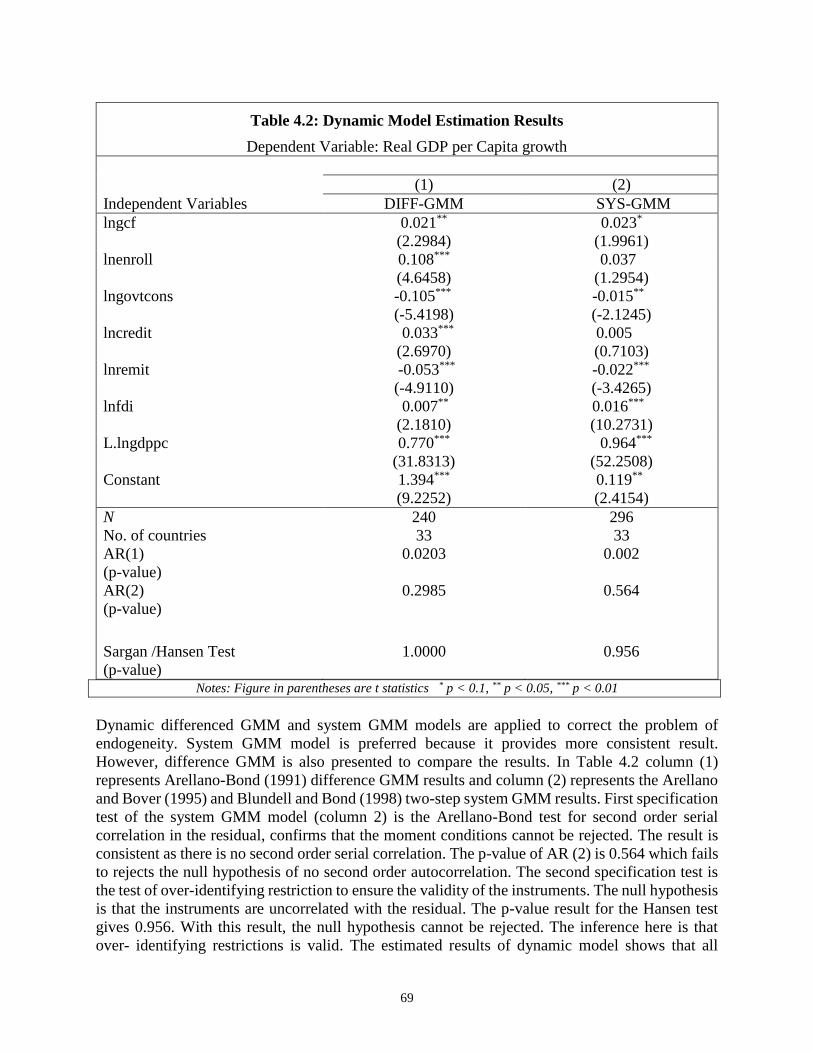
Table 4.2: Dynamic Model Estimation Results

Dependent Variable: Real GDP per Capita growth

(1) (2)

Independent Variables DIFF-GMM SYS-GMM

lngcf 0.021** 0.023*

(2.2984) (1.9961)

lnenroll 0.108*** 0.037

(4.6458) (1.2954)

lngovtcons -0.105*** -0.015**

(-5.4198) (-2.1245)

lncredit 0.033*** 0.005

(2.6970) (0.7103)

lnremit -0.053*** -0.022***

(-4.9110) (-3.4265)

lnfdi 0.007** 0.016***

(2.1810) (10.2731)

L.lngdppc 0.770*** 0.964***

(31.8313) (52.2508)

Constant 1.394*** 0.119**

(9.2252) (2.4154)

N 240 296

No. of countries 33 33

AR(1)

(p-value)

0.0203 0.002

AR(2)

(p-value)

0.2985 0.564

Sargan /Hansen Test

(p-value)

1.0000 0.956

Notes: Figure in parentheses are t statistics * p < 0.1, ** p < 0.05, *** p < 0.01

Dynamic differenced GMM and system GMM models are applied to correct the problem of

endogeneity. System GMM model is preferred because it provides more consistent result.

However, difference GMM is also presented to compare the results. In Table 4.2 column (1)

represents Arellano-Bond (1991) difference GMM results and column (2) represents the Arellano

and Bover (1995) and Blundell and Bond (1998) two-step system GMM results. First specification

test of the system GMM model (column 2) is the Arellano-Bond test for second order serial

correlation in the residual, confirms that the moment conditions cannot be rejected. The result is

consistent as there is no second order serial correlation. The p-value of AR (2) is 0.564 which fails

to rejects the null hypothesis of no second order autocorrelation. The second specification test is

the test of over-identifying restriction to ensure the validity of the instruments. The null hypothesis

is that the instruments are uncorrelated with the residual. The p-value result for the Hansen test

gives 0.956. With this result, the null hypothesis cannot be rejected. The inference here is that

over- identifying restrictions is valid. The estimated results of dynamic model shows that all

70

control variables; i.e. gross capital formation as a share of GDP, secondary school enrollment ratio,

government consumption and domestic credit as a share of GDP carry the expected sign which

are consistent with the theory. The positive coefficient associated with lagged dependent variable

does not support the conditional convergence hypothesis for the developing countries in sample.

The result indicates a case of non-convergence that means country with higher level of per capita

income will grow faster than the countries with low level of per capita income (Fayissa and Nsiah,

2008).

The physical capital investment measured by gross capital formation as a share of GDP is

statistically significant in dynamic model. Ceteris paribus, an increase in physical capital of about

10 percent would result in a 0.23 percent increase in economic growth. The coefficient magnitude

is modest in dynamic model, compared to the finding in static model, which reported a 0.82 percent

increase in economic growth following a 10% rise in physical capital. The school enrollment ratio

(lnenroll) has the expected positive sign but not statistically significant in dynamic specification

system GMM of the growth model. In the static model, school enrollment was also positively

related to economic growth and the coefficient was highly significant at 1% significant level. The

result on government consumption expenditure is consistent with the theory and static model. The

coefficient is statistically significant and has a negative sign, suggesting a negative relationship

between government consumption and economic growth. Ceteris paribus, a 10 percent increase in

government consumption expenditure is associated with a 0.15 percent decrease in economic

growth. Financial market development was measured by domestic credit. The dynamic model

establishes a positive relationship with economic growth. The static model also found a positive

relationship. However, it is not statistically significant in the dynamic model, but was statistically

significant in the static model.

The finding on remittances addresses one of the key questions in this study. The analysis

establishes that the coefficient for remittance is statistically significant and also that it has a

negative relationship with economic growth. In static model, we also got a similar result. This

result suggests that the direct impact of remittance on economic growth appears to be negative

across the developing countries in sample over the study period. The dynamic model shows that

a 10 percent increase in remittances (remittance to GDP ratio) leads to a 0.22 percent decrease in

economic growth. In the static model, the coefficient for remittances was statistically insignificant

under both fixed effect and random effect. However, the model was not corrected for endogeniety.

In the dynamic model, the endogeniety problem was corrected by using GMM and it became

significant.

The result on remittances is consistent with Chami et al.(2005) and Bettini and Zazzaro (2008).

Bettini and Zazzaro (2008) explained that the partial reason why Remittances have not inspired

economic growth is that they are generally not aimed to serve as investments but rather as social

insurance to help family members finance the purchase of life’s necessities. According to Chami

et al.(2005), remittance would create moral hazard and lessen the incentive to work. Ascosta and

lartey (2009) found that an increase in remittance may hinder growth by reducing labor supply and

increasing consumption demand biased towards non-tradable. There would be an increase in

import of goods which may eventually cause “Dutch disease”.

The negative result on remittance suggests that Remittances should not be considered as a key

instrument of economic growth. If most of the Remittances are consumed rather than invested then

71

direct impact of Remittances on growth would not be gained. Though Remittances alleviate

poverty with additional income for consumption and investment; it could harm a country by

exchange rate appreciation and inflation. Other possible reasons of negative impact of Remittances

are labor force shrink and increase in reservation wage. However there are some indirect effects

of Remittances which are not usually captured by remittance related studies. Identifying the proper

channels through which Remittances can influence economic growth would help developing

countries to find effective use of Remittances.

The other main research question in this study was to examine the impact of FDI on economic

growth. In order to test sensitivity of the results different specification of both static models and

dynamic models are applied. The results from the dynamic model show that FDI has a positive

and statistically significant association with economic growth. The result indicates that a 10

percent increase in FDI (FDI to GDP ratio) leads to a 0.16 percent increase in economic growth

across the developing countries in sample. The static model also showed a positive relationship

between FDI and economic growth. The only difference is on the magnitude of the coefficient. A

10 percent increase in FDI was associated with a 0.13percent rise in economic growth. There are

a couple of channels through which FDI may impact growth. FDI develops new foreign technology

or import new intermediary goods in the production function. This accelerates economic growth

by fueling capital accumulation in capital scarce developing countries. FDI accelerates economic

growth by contributing to the accumulation of human capital. It does so by training laborers or

absorbing technology and new management techniques.

5.0 Conclusion

Researchers differ widely about the contribution of international capital flows on economic

growth. Other researchers argue that international capital flows impact on economic growth

positively, while others doubt the effect of international capital flows on economic growth.

Remittances and FDI are among the key international capital flows to developing countries. This

study has cast light on this debate by investigating the impact of Remittances and FDI on economic

growth of selected developing countries. I found that the coefficient for remittance is statistically

significant and there is a negative relationship between remittance and real GDP per capita across

the developing countries in sample over the study period. It was further established that a 10

percent increase in remittances (remittance to GDP ratio) decreases real GDP per capita by 0.22

percent for the developing countries in sample over the study period. The result suggests a

conclusion that a significant proportion of Remittances are channeled to the non-productive uses

and the motive of remitting to the home country economies is mostly altruistic rather than profit

driven. Several empirical studies also have found negative impact of Remittances on growth

(Chami et al., 2005). The insignificant magnitude of Remittances in the static model for the

developing countries in sample indicates that remittance is used to meet household non-productive

consumption demands of home economies which do not directly contribute to the economic

growth. Thus only remittance flow is not important for a country but at the same time ensuring

proper utilization and where and how it is spent is equally important. The productive use of

remittance flows demands active role of government and policy makers to ensure that this financial

flow is directed towards productive sectors. On the other hand, the empirical result on FDI shows

some evidence that FDI is positively associated with economic growth across the developing

countries in sample over the study period. A 10 percent increase in FDI (FDI to GDP ratio) increase

real GDP per capita by 0.16 percent. On FDI, it can be concluded that FDI contributes to the

72

advancement of developing countries. However, this potential positive effect of FDI on economic

growth depends on both country-specific characteristics and gaining a certain threshold level of

development by the recipient economy to give it enough absorptive capacity to benefit from the

FDI.At the end, increase of Remittances and FDI in quantity can enhances economic growth only

under some conditions. Such as- better human resources, export-oriented strategy, diversified

economic and export structure and stable macroeconomic environment. Based on the level of

economic development each country should focus on their economic growth by taking steps to

improve the level of human capital, macroeconomic stability and reducing corruption and then

encourage FDI.

Limitations and Suggestions for Future Research

This study extends the existing literatures on impact of Remittances and FDI on economic growth

of developing countries. This study is conducted on cross- country analysis due to limitations of

data availability. Cross-country studies are only the means of testing the validity of generalization.

Country specific study is needed to design country specific policies. Future study will focus on the

regional and country specific analysis of Remittances and FDI.

5.0 References

Abdih, Y., Chami, R., Dagher, J. & Montiel, P. (2012). Remittances and institutions: Are

Remittances a Curse? World Development, 40(4), 657–666.

Acosta, P., Fajnzylber,P. & Lopez, J.H. (2007). The impact of Remittances on Poverty and Human

Capital: Evidence from Latin American Household Surveys. In: Özden Ç and Schiff M, eds.

International Migration, Economic Development and Policy. World Bank and Palgrave

Macmillan: 59–98. Washington (DC) and London.

Acosta, P., Lartey, E. & Mandelmans, F. (2009). Remittances and the Dutch Disease. Working

Paper 2007-8, Federal Reserve Bank of Atlanta.

Akinolo. (2004). Foreign Direct Investment and Growth in Nigeria: An Empirical Investigation.

Journal of Policy Modelling, 26627-639.

Adolfo B., Chami R., Fullenkamp C., Gapen M., & Peter M. (2009). Do Workers’ Remittances

Promote Economic Growth? IMF Working Paper No. WP/09/153.

Agosin, M. & Mayer, R. (2000). Foreign Direct Investment: Does It Crowd in Domestic

Investment? United Nations Conference on Trade and Development Geneva, Switzerland,

Working Paper, 146.

Agosin, M., & Machado, A. (2006). Openness and the international allocation of foreign direct

investment. Economic and Sector Studies Series, RE2-06-004. Washington, D.C.: Inter-

American Development Bank.

Ayanwale, A.B. (2007). FDI and Economic Growth: Evidence from Nigeria, Nairobi, African

Economic Research Consortium Paper, 165.

Arellano, M., & Bond, S. (1991) .Some tests of specification for panel data: Monte Carlo Evidence

and an application to employment equations. The review of economic studies, 58(2), 277-

297.

Azam, M. & Khan, A. (2011). Workers’ Remittances and Economic Growth: Evidence from

Azerbaijan and Armenia. Global Journal of Human Social Science, 11(7).

73

Bettin,G., & Zazzaro,A. (2008). Remittances and Financial Development: Substitutes or

Complements in Economic Growth? Working Paper 28, Money and Finance Research

Group.

Barajas, A., Chami, R., Fullenkamp, C., Gapen, M., & Montiel, P. (2009). Do workers’

Remittances promote economic growth? Working Paper (153), IMF.

Barro, R., & Sala-i-Martin, X. (2004). Economic Growth. 2nd ed. Cambridge, MA, U.S.A: MIT

Press.

Borensztein, E., De Gregorio, J., & Lee, J.W., (1998). How Does Foreign Direct Investments

Affect Economic Growth?Journal of International Economics, Vol. 45.

Buch, C. M., & Kuckulenz, A. (2004). Worker Remittances and Capital Flows to Developing

Countries. Centre for European Economic Research, Discussion Paper ,No. 04-31.

Catrinescu, N., Leon-Ledesma, M., Piracha, M., & Quillin, B. (2009). Remittances, Institutions,

and Economic Growth. World Development. 37(1), 81–92.

Chami,R., Fullenkamp, C., & Jahjah, S. (2005).Are Immigrant Remittances Flows a Source of

Capital Development? IMF Staff Papers, 52(1), IMF.

Chami R. et al. (2008). Macroeconomic Consequences of Remittances. International Monetary

Fund. Washington (DC).

Das, A. & Chowdhury, M. (2011).Remittances and GDP Dynamics in 11 Developing Countries:

Evidence from Panel Cointegration and PMG Techniques. Romanian Economic Journal,

14, 3-24.

De Mello, L.R. (1997). Foreign Direct Investment in Developing Countries and Growth: A

Selective Survey. The Journal of Development Studies, 34, 1-34.

Driffield , N. & Jones C. (2013). Impact of FDI, ODA and Migrant Remittances on Economic

Growth in Developing Countries: A Systems Approach. European Journal of Development

Research, 25(2) 173–196.

Fayissa, B. & Nsiah, C. (2010). Can Remittances Spur Economic Growth and Development?

Evidence from Latin American Countries (LACs). Middle Tennessee State

University,Working Paper Series, March 2010.

Gapen, M. T., Barajas, A., Chami, R., Montiel, P., & Fullenkamp, C. (2009). Do workers'

remittances promote economic growth?. International Monetary Fund.

Glytsos, N. P. (2005). The contribution of Remittances to growth, A Dynamic Approach and

Empirical Analysis. Journal of Economic Studies, 32(6), 468-496.

Giuliano,P., & Ruiz-Arranz M. (2009). Remittances, Financial Development, and Growth. Journal

of Development Economics. 90(1), 144–152.

Greene, William H.(2003).Econometric Analysis(5th ed.).Upper Saddle River, N.J.: Prentice Hall.

Gupta, S., Catherine P., & Smita W. (2007). Impact of Remittances on Poverty and Financial

Development in Sub-Saharan Africa. IMF Working Paper.

Gracia–Fuentes, Pablo A. (2009). Remittances, Foreign Direct Investment and Economic Growth

in Latin America and the Caribbean. In Louisiana State University and Agricultural and

Mechanical College.

Hermes, N., & Lensink, R. (2003). Foreign Direct Investment, Financial Development and

Economic Growth. The Journal of Development Studies, 40, 142-163.

Jongwanich, J. (2007). Workers’ Remittances, Economic Growth and Poverty in Developing Asia

and the Pacific Countries. UNESCAP, Working Papers, WP/07/01.

Kim, N. (2007). The impact of Remittances on labor supply: The case of Jamaica. Policy Research

Working Paper Series, 4120. World Bank. Washington (DC).

74

Li, X., & Liu, X. (2005). Foreign Direct Investment and Economic Growth: An Increasing

Endogenous Relationship. World Development, 33(3), 393-407.

Lee, J. W., Baimukhamedova G. S., & Akhmetova S. (2009). The Effects of Foreign Direct

Investment on Economic Growth of A Developing Country: From Kazakhstan. Allied

Academies International Conference. Academy for Economics and Economic Education,

12(2), 22-27.

Mansoor, A. and Quillin, B. (2006).Migration and Remittances: Eastern Europe and the Former

Soviet Union, World Bank.

Mencinger, J. (2003). Does Foreign Direct Investment Always Enhance Economic Growth?

Kyklos, 56(4), 491-509.

Mo, P. H. (2001). Corruption and economic growth. Journal of Comparative Economics, 29(1),

66-79.

Mottaleb, K.A. (2007). Determinants of Foreign Direct Investment and Its Impact on Economic

Growth in Developing Countries,MPRA Paper 9457, University Library of Munich.

Misztal, P. (2010). Foreign Direct Investments, As a Factor for Economic Growth in Romania.

Journal of Advanced Studies in Finance,1(1),72-82.

Mundell, R. (1957). International Trade and Factor Mobility. American Economic Review, 47,

321-335.

Nair-Reichert, U. & Weinhold, D. (2001). Causality Tests for Cross-Country Panels: A New Look

at FDI and Economic Growth in Developing Countries. Oxford Bulletin of Economics and

Statistics, 63, 153-171.

Ratha, D. (2003).Workers’ Remittances: An Important and Stable Source of External

Development Finance. Global Development Finance 2003, World Bank.

Ratha, D. & Mohapatra, S. (2007).Increasing the Macroeconomic Impact of Remittances on

Development. Development Prospects Group 2007, World Bank.

Ratha,D, Mohapatra, S. & Silwal, A. (2009). Migration and Remittance Trends 2009: A better-t

han-expected outcome so far, but significant risks ahead. The Migration and Development

Brief 11, World Bank.

Ratha, D., Mohapatra, S., & Silwal, A. (2010a). Outlook for Remittance Flows 2010-11:

Remittance flows to developing countries remained resilient in 2009, expected to recover

during 2010-11. Migration and Development Brief 12, World Bank.

Ratha, D., Mohapatra, S., & Silwal, A. (2010b). Outlook for Remittance Flows 2011-12: Recovery

after the crisis, but risks lie ahead. Migration and Development Brief 13, World Bank.

Ratha, D. (2013). The impact of Remittances on economic growth and poverty reduction.

Washington, DC: Migration Policy Institute.

Roodman, D. (2009). How to do xtabond2: An Introduction to Difference and System GMM in

Stata. The STATA Journal, 9(1), 86-136.

Romer, D. (2006). Advanced macroeconomics. 3rd ed. New York: McGraw-Hill/Irwin.

Romer, P. (1990). Endogenous Technological Change. The Journal of Political Economy.

98(5), S71‐S102.

Sarkar, P. (2007). Does Foreign Direct Investment Promote Growth? Panel Data and Time Series

Evidence from Less Developed Countries, 1970-2002. Munich Personal RePEc.

Archive.W/ P No. 5176.

Siddique, A., Selvanathan, E. A. & Selvanathan, S. (2010). Remittances and Economic Growth:

Empirical Evidence from Bangladesh, India and Sri Lanka. University of Western Australia

Discussion Paper 10.27

75

Solow, R.M. (1956). A Contribution to the Theory of Economic Growth. Quarterly Journal of

Economics 70, 65-94.

Teboul, R., & Moustier, E., (2001). Foreign aid and economic growth: the case of the countries

south Mediterranean. Applied Economics Letters, 8, 187-190.

Temple, J. (1999). The new growth evidence. Journal of Economic Literature, 37, 112-156.

Thomas, H., Li X., & Liu, X. (2008). Ownership Structure and Now Product Development

in Transnational Corporation in China, Transnational Corporations, 17(2), 17-44.

Vijayakumar, N. Sridharan, P. & Rao, K.C.S. (2010).Determinants of FDI in BRICS

Countries: A Panel Analysis. International Journal of Business Science and Applied

Management, 5 (3),1-13.

Wooldridge, J. (2002). Econometrics Analysis of Cross section and Panel Data. MIT, U.S.A.

Ziesemer, THW. (2012). Worker Remittances, Migration, Accumulation and Growth in

Poor Developing Countries: Survey and Analysis of Direct and Indirect Effects. Economic

Modelling, 29(2), 103–11.

Zilinske, A. (2010) Negative and Positive Effects of Foreign Direct Investment Economics and

Management. Vol 15. pp 332-336

6.0 Appendix

A.1 List of the Countries

Countries Code countries: Code countries: Code

Azerbaijan AZE EL Salvador SLV Morocco MAR

Bangladesh BGD Guatemala GTM Mozambique MOZ

Belize BLZ Honduras HND Nigeria NGA

Bolivia BOL India IND Pakistan PAK

Bulgaria BGR Jordan JOR Panama PAN

Cambodia KHM Kyrgyz

Republic

KGZ

Peru PER

China CHN Lesotho LSO Philippines PHL

Colombia COL Macedonia,

FYR

MKD Rwanda RWA

Dominican

Republic

DOM Mali MLI Togo TGO

Ecuador ECU Mexico MEX

Tunisia TUN

Egypt EGY Moldova MDA

Turkey TUR

76

A.2 Definition of Variables and Data sources

Variable Description Source

The growth of real GDP per capita.

Measured as the growth of real per

capita GDP in constant (2005) U.S.

dollars.

The World Bank,

World Development Indicators

(WDI) database

The log of gross fixed capital

formation as a percentage of GDP

used here as a proxy for investment

in physical capital.

The World Bank,

World Development

Indicators(WDI) database

Log of Secondary school

enrollment (percentage of gross) is

used as a proxy for human capital.

The World Bank,

World Development

Indicators(WDI) database

Log of General Government final

consumption expenditure as a

percentage of GDP used as a proxy

for fiscal policy

The World Bank,

World Development

Indicators(WDI) database

Log of Domestic credit as a

percentage of GDP is used as a

proxy for financial market

development.

The World Bank,

World Development

Indicators(WDI) database

Log Remittances as a percentage of

GDP

The World Bank,

World Development

Indicators(WDI) database

Log of net Foreign Direct

Investment inflows as a percentage

of GDP

The World Bank,

World Development

Indicators(WDI) database

77

A.3 Summary Statistics

Variables Obs.(N) Mean Std. Dev Min Max

lngdppc 396 7.283688 .9166048 5.350497 9.028377

lngcf 396 3.066477 .3354499 1.698733 5.028666

lnenroll 339 4.059324 .5118799 1.80029 4.600397

lngovtcons 395 2.516074 .403231 1.241377 3.676331

lncredit 386 3.363053 .6848216 1.342607 4.866944

lnremit 394 1.432882 1.171204 -1.996465 4.127016

lnfdi 390 1.084779 .9910634 -2.20706 3.809987

A.4 Correlation Matrix

lngdppc

ln g

cf

lnen

roll

lngovtc

ons

lncr

edit

lnre

mit

lnfd

i

lngdppc 1

lngcf 0.1510* 1

lnenroll 0.7004* 0.2169* 1

lngovtcons 0.2046* 0.3068* 0.2839* 1

lncredit 0.4456* 0.3322* 0.4177* 0.1937* 1

lnremit -0.1280* 0.0328 0.1153* 0.2286* -0.0317 1

lnfdi 0.2120* 0.2518* 0.2372* 0.2576* 0.1160* 0.1323* 1

*Significance at 5% level