impact of cross-border transport infrastructure on trade ... · impact of cross-border transport...

- 1 -

ADB Institute Discussion Paper No. 48

Impact of Cross-border Transport Infrastructure on Trade and Investment in the GMS

Manabu Fujimura and Christopher Edmonds

March 2006

The authors are Professor of Economics at Aoyama Gakuin University, and Fellow, Research Program at the East-West Center (and Affiliate Graduate Faculty of the Economics Department at University of Hawaii- Manoa), respectively. The views expressed in this paper are the views of the authors and do not necessarily reflect the view or policies of the Asian Development Bank Institute nor the Asian Development Bank. Names of countries or economies mentioned are chosen by the author/s, in the exercise of his/her/their academic freedom, and the Institute is in no way responsible for such usage.

- 2 -

Introduction This paper investigates the impact of cross-border transport infrastructure on the economies of the Greater Mekong Subregion (GMS).1 Cross-border and domestic transport infrastructure together can reduce trade costs and lead directly to increased trade and investment. Reduced trade costs can also indirectly induce increased foreign direct investment (FDI) mainly through intra-firm vertical integration across borders that exploits the comparative advantages of each location, and in turn, such increases in FDI can further increase regional trade, adding to the direct effect of trade expansion. This defines a virtuous triangle of mutually reinforcing effects between cross-border infrastructure development, trade, and investment, the final effects of which are higher economic growth and—if necessary institutions and policies are in place to ensure the poor take part in this growth—poverty reduction. Increased trade and growth also expand the fiscal resources available to governments thereby enabling consideration of new policy options (e.g. investments in education, health, or social protection systems). The intricate impacts of cross-border transport infrastructure investments and associated institutional efforts for trade facilitation cannot be adequately captured by traditional techniques of project accounting, which focus on first-order outcomes directly linked to infrastructure development. In addition, analysis of the international political economy and the distribution of benefits and costs associated with cross-border transport infrastructure projects across the two or more countries raise complexities not typically encountered in single-country projects, and making such projects prone to actual and perceived inequities between the parties. Inequalities in the incidence of benefits and costs across parties, in turn, call for transparent compensation schemes among the participating members or some self-enforcing mechanisms and third-party coordination in order for projects that cross national boundaries to be accepted by the countries involved. Attempts to devise such mechanisms must however be preceded by a clear understanding of the relationship between infrastructure development, trade, and FDI. This paper seeks to contribute to the understanding of the economic impacts of cross-border infrastructure projects by investigating and quantifying trade creation and investment facilitation effects of cross-border infrastructure in the GMS. The motivation and more detailed background of this research are discussed in Fujimura (2004). Literature review Three strands of literature contribute to the current research. First, the literature pertaining to the “new” economic geography that has flourished since 1990s makes increasingly clear the importance of geography in explaining patterns of trade and economic development. For example, access to sea and distance to major markets have been shown to have a strong impact on shipping costs, which in turn, strongly influence the success developing countries achieve in global markets for manufactured 1 Members of GMS are Cambodia, Lao PDR, Myanmar, Thailand, Viet Nam and two southern provinces of the People’s Republic of China: Yunnan and Guanxi. Guanxi Province joined the GMS in 2005. Due to scarcity of detailed data documented (e.g., in Guanxi Statistical Yearbooks), particularly on transport infrastructure, empirical analyses in this research had to exclude data specific to Guanxi Province.

- 3 -

exports and ultimately in their achievements in terms of economic growth (e.g. Limao and Venables, 2001). Countries suffering multiple geographical handicaps such as landlocked status, an absence of navigable rivers and lakes, or tropical or desert ecology, tend to be among the poorest in the world. Though these correlations are commonsensical, economic geographers have contributed quantitative results by combining new tools in Geographical Information Systems (GIS) with empirical economic modeling (e.g. Radelet and Sachs, 1998, and Redding and Venables, 2004). These papers have documented a strong negative empirical relationship between transport costs and economic growth controlling for the other variables that would be expected to influence growth. In the context of GMS, the relative poverty of Lao PDR has long been understood as at least a partial result of the country’s landlocked status. Empirical evidence in this literature suggests there is much potential for cross-border road infrastructure and associated institutional arrangements to benefit economies that are not endowed with geographic characteristics favorable to economic development. Second, the “new” trade literature that incorporates the presence of imperfect competition in standard trade theory derives many policy implications for prompting trade and growth that are not predicted in the standard neoclassical trade models (i.e. Hecksher-Ohlin-Samuelson type models). For example, Markusen and Venables (2000) find that the presence of transaction/trade costs and increasing returns to scale in production may create incentives for production agglomeration in particular markets. On the other hand, papers in this literature have also found that multinational firms can gain from intra-firm trade by integrating production processes located in different countries with varied comparative advantage, which reduces the tendencies towards production agglomeration. If the advantages of production integration across different countries outweigh those from agglomeration, then following this reasoning, reductions in transport costs would make FDI complementary to trade.

Third, the longstanding but recently revived empirical literature examining the relationship between the level of trade, trade openness, and broader economic growth suggest a positive effect of increased trade and openness on economic growth.2 These studies often share an understanding that one of the common threads in the economic successes of the “East Asian Miracle” has been the trade openness of these economies, and a virtuous cycle of increased trade, economic growth, and FDI in export-oriented manufacturing industries based on comparative advantage. This literature suggests the possibility of a trade-FDI nexus in GMS that can be induced by investments in cross-border transport infrastructure.3 GMS economies have the potential to benefit significantly from regional economic integration in the areas of trade and investment though the development of improved cross-border infrastructure. Easier trade and financial transactions can enable these economies to better exploit their comparative advantages, to gain from increased specialization and scale economies in production, and more generally to enhance their complementary economic relationships. For example, Thailand currently provides a significant share of the manufactured goods demanded by Lao consumers while it purchases a significant share of Lao PDR’s resource-based exports (e.g. hydroelectric power and timber).

2 See, for example, Edwards (1993), Harrison (1996), Frankel and Romer (1999), and Dollar and Kraay (2004). 3 Trade-FDI nexus in line with the argument here has been well researched in the context of East Asia’s economic integration: e.g., Fukao, Ishido and Ito (2003) and Urata (2001).

- 4 -

Issue of benefit-cost incidence Notwithstanding the aggregate benefits expected from the development of cross-border infrastructure, the benefits and costs of such investments are unlikely to accrue equitably across involved countries. This is particularly likely in instances like the GMS where the countries involved are disparate in economic size and in their level of economic development. Problems in the incidence of benefits and costs of trade liberalization and trade integration across large and small economies are well discussed in the trade literature.4 This literature also highlights the prominence of asymmetries in bargaining power and inequities in distribution of trade benefits when trade integration is pursued between large and small economies.

The greater complexity of cross-border infrastructure projects that require coordination between multiple bureaucracies, compensation/cost-sharing between affected countries, and synchronizing project work across different countries and contractors can make them riskier than projects based in a single country. Participating countries face different political and economic circumstances and cycles, and often have starkly contrasting abilities to negotiate and implement projects (Ferroni, 2002). The task of correctly accounting for the economic and financial benefits and costs of cross-border infrastructure projects is also made correspondingly more difficult by these project characteristics.5 Asymmetries in the benefit-cost incidence across countries must be delineated and addressed in the design and implementation of investments in cross-border transport infrastructure, such as those currently underway in the GMS. For example, in the case of the North-South Economic Corridor linking Kunming (Yunnan Province of the People’s Republic of China) to Chiang Rai (Thailand), much of the road runs through northern Lao PDR. However, the road is expected to bring greater economic benefits to Thailand and Yunnan Province through enhanced trade between these two large economies with their large industrial and agricultural sectors, and is expected to have relatively little effect on Laotian trade. However, many of the environmental and social externalities associated with the road’s construction and operation (e.g., greater difficulty of travel while the road is under construction, encroachment on fragile forests and indigenous communities, risks of vehicle collisions to people and animals living along the road, and increased transmission of disease associated with anticipated increase in transit visitors), will likely be borne by stakeholders in Lao PDR. Accordingly, it is not surprising that the Chinese and Thai governments have joined ADB in financing the Lao portion of the North-South Economic Corridor’s road upgrading at concessional terms to the Lao government and the project proposal includes components to provide technical assistance to mitigate the effects of anticipated adverse environmental and social impacts of the road. Research questions With the above as background, this paper attempts to investigate the relationship between cross-border infrastructure, trade, and FDI flows between countries in the GMS. Our interest extends to a number of empirical questions considered to be of importance 4 See, for example, McLaren (1996) and Lee et al. (2004).5 A methodological framework for economic analysis of sub-regional projects such as Adhikari and Weiss (1999) has been available, but operational practice has been limited to date due to data constraints.

- 5 -

in the context of ongoing road infrastructure development in the GMS.

• What are the empirical relationships between measures of cross-border road infrastructure, trade, and FDI between GMS countries historically (since the mid-1980s)?

• Can additional reductions in trade costs and increases in trade flows associated

with investments in cross-border road infrastructure be found, and (if found) what is the magnitude of these associated trade creation effects?

• Do reductions in trade costs lead to increased foreign direct investment (FDI)

and to what extent can trade creation be attributed to increased FDI flows? In attempting to answer these questions, we hope to gain insight into the value of regional economic benefits associated with the increased regional trade and the distribution of such benefits among the GMS members. Research findings regarding these questions would hold promise in terms of fostering the design of cross-border infrastructure in the future, and in developing coordination and compensation arrangements among the involved economies. Analytical approach and estimation models Our analytical approach is adapted from that applied in Limao and Venables (2001) and applies a gravity model to predict bilateral trade and FDI flows by each pair of GMS members.6 Estimation parameters of particular interest are the responses of trade and FDI to various transport cost factors including cross-border road infrastructure, and the determinants of investments in cross-border transport infrastructure. Accordingly, the empirical analysis centers around three functional relationships: a trade equation, an FDI equation, and a cross-border road infrastructure equation. 1. Trade equation: Xij =X(Yi,Yj ,Ri,Rj,Fij ,ωij)

- Xij : exports of country i to country j via land - Yi , Yj : vector of fixed or predetermined characteristics of country i (j) related to

trade such as distance, economic size (GDP), population, land area, domestic road infrastructure, and similar variables routinely used in gravity model estimates.

- Fij : country i’s foreign direct investment from country j. - Ri , Rj : vector of variables measuring border area and general domestic road

infrastructure of country i (j ). - ωij : other factors not accounted for (model error). The trade equation incorporates standard variables used in gravity models plus variables of particular interest in this research (i.e., measures of cross border and domestic road infrastructure, and FDI from the trading partners). Other factors seen as important in driving levels of bilateral trade, which are elements in vectors Yi and Yj) are

6 Departing from Limao and Venables (ibid.), we omit estimation of a transport cost equation which could not be estimated for the case of overland transport of goods within the GMS due to data limitations. See the Appendix for details.

- 6 -

tariff rates, inflation rates, and a broad characterization of the export/import environment in the countries. A principal aim in the analysis is to quantify the “incremental effect” of cross-border road infrastructure on trade relative to the effect of domestic road infrastructure. Trade is envisioned to be a function of both the quality of road infrastructure generally in each country and of road infrastructure in border areas in particular. Both road indicators are seen as being relevant to determining the flows of goods and raw materials between the countries since they form part of the transport network used to connect markets. In the next subsection of the paper we discuss our expectations regarding the signs of estimation coefficients, while further details concerning the definition, measurement, and sources of data used are left to the notes to Table 1 and the Appendix. The value of exports between pairs of GMS countries is of interest both because of our interest in exploring the empirical relationship between cross-border infrastructure and trade, and because trade levels are broadly indicative of transportation costs. While reliable information on overland transport costs is generally unavailable for GMS countries, examination of overland trade flows can provide some insight into changing overland transport costs in the GMS. 2. FDI equation: Fij = F(Yi, Yj, zi ,Ri,Rj,Xij,εij)

- Fij : country i's foreign direct investment inflow from country j - Yi , Yj : vector of characteristics of country i and j (same as in trade equation) - zi : vector of characteristics related to country i’s investment climate - Ri , Rj : vector of variables measuring border area and general domestic road

infrastructure of country i (j). - Xij : exports of country i to country j via land - εij : other factors not accounted for (model error). The FDI equation specifies capital flows as being determined by several factors that also appear in the trade equation (e.g. economy size and resources, inflation rate, tariff rates). Of particular interest is the relative contribution of general road infrastructure and road infrastructure in the border area. In addition, FDI is viewed as being influenced by the volume of trade and the FDI and trade environment in the FDI-recipient country. 3. Cross border infrastructure equation: Roadij = R(Yi , Yj , zi , Ri , Rj , Xij , υij ) - Roadij : measure of the stock and quality of country i’s road infrastructure in the border

area with country j. - Yi , Yj : characteristics of country i and j (same as in transport cost equation). - zi : vector of characteristics related to country i’s trade and investment climate - Ri ,Rj : vectors of variables measuring general domestic road infrastructure of

country i/j. - Xij : exports of country i to country j via land - υij : other factors not accounted for (model error). Lastly, we define the cross-border infrastructure equation wherein structural characteristics of the country, the investment climate, the level of trade and FDI flows, and the quality of roads in the country in general are related to cross-border road infrastructure. The main reason for including this equation in our analysis is to examine

- 7 -

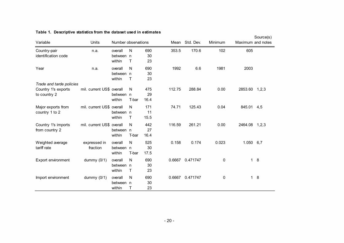
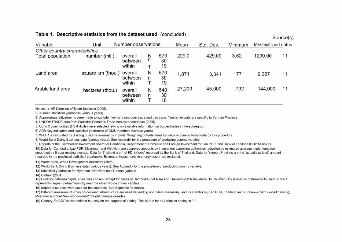
the possibility of reverse causality in the construction of cross-border infrastructure, i.e., this equation allows for the possibility that the construction of roads in border areas is a response to—rather than a cause of—trade and FDI flows. Dataset, estimation model, and estimation procedures Our dataset is formed from a cross-sectional time series of data available for GMS member economies for the period of 1981-2003. Observations in the dataset are defined at the country-pair level over time. In all, 30 country pairs can be formed across the 6 GMS member countries (i.e., Cambodia-Lao PDR, Cambodia-Myanmar,…, Yunnan (PRC)-Thailand, Yunnan (PRC)-Viet Nam). Descriptive statistics from the dataset along with details on the data sources and definitions of variables are summarized in Table 1. Because the resulting dataset captures the value of variables for the country-pair over time, Table 1 presents the number of observations of each variable and country-pair over time (years). Nonetheless, due to the small number of GMS countries and relatively short time period for which most data are available for some GMS countries, our analysis faced challenges in model estimation. For example, data at the start of our panel is available for only a few GMS countries because some of the poorer GMS countries suffered major military conflicts in the 1970s and were only establishing or recovering their national statistical capacity in the early 1980’s. The Appendix provides detailed explanations of key variables and of the sources of data. Two key concepts are cross border infrastructure and domestic road infrastructure. For the former we use as a proxy the road density in the provinces that share a border with a GMS neighbor. Where there is more than one such provinces we take an average. For the latter we use the average road density of all provinces in a country that do not share a border with a GMS neighbor. Limitations in available data representing transport costs in the GMS made us forgo the estimation of the determinants of transport costs (as in Limao and Venables, op. cit.), so instead we estimate the trade and FDI equations with road infrastructure being one of the explanatory variables. Also, quantification of indirect economic impacts that come through trade and FDI is judged premature and is deferred until a more rigorous structure of the trade-FDI nexus can be modeled and supported by improved data.7

Following the general functional relationships defined above, our estimation models define total exports, FDI, and investments in cross-border infrastructure (Xij) from country i to country j in time t as:

)( ijijtijjtitjijtitijt uDNNHHYAYX MEMEME += εφγγββαα

where: Yit, Yjt are the gross domestic products of countries i and j in year t; Hi, Hj are the geographic sizes of countries i and j; Nit, Njt are the populations of countries i and j in year t; Dij is the distance between (the capitals of) countries i and j; εijt is the regular error term; uij is an error component specific to country-pair ij ; A is a constant;

7 Econometric estimation of a simultaneous system of equations (trade, FDI, cross-border infrastructure) is not feasible, mainly due to the limited sample size available.

- 8 -

and the following signs are hypothesized for the estimation parameters: αE,αM >0; and βE, βM, γE, γM, φ < 0.

In logarithmic form, we have:

ln Xijt=ln A+αE ln Yit+αM ln Yjt+βE ln Hi+βM ln Hj+γE lnNit,+γM Njt+φln Dij+ln εijt+ln uij,

Country GDP is considered a key variable in the base gravity model, and larger economies are expected to engage in greater trade. Trade is viewed as being positively affected by the economic mass of the trading partners and negatively affected by the distance between them. Other factors also act against the ‘gravity like’ forces of economy size. Geographic area and population size are factors expected to reduce trade orientation by increasing the size of the domestic market and making economic activity more inwardly oriented. Additional variables, such as indicators of cultural affinity and sharing contiguous borders are usually added to empirical gravity models. Using this as base model, we can add variables for cross-border road infrastructure and FDI to consider the effect of these two variables on trade flows—controlling for the standard variables treated in the gravity model—and providing our basis for estimating the trade equation outlined above.

Models are estimated using the Generalized Least Squares (GLS) Random Effects estimator for cross sectional time series data. We forego detailed discussion of technical details pertaining to the estimation procedure except to note that estimation coefficients reflect a weighted average of the cross-sectional and time-series association between the dependent and independent variables included, and the weighting is defined by the estimation parameter theta—which is reported for our panel estimates.8

The overall statistical significance of the estimation models is tested using a Wald Chi-square test, while the need for the random effects estimator as opposed to treating the cross-sectional time-series data simply as a cross-section and applying regular GLS is tested through a Breusch and Pagan Langranian Multiplier test (technical details are also in Green, 2003). The Wald Chi-square test indicates the probability of a false rejection of the null hypotheses that the model has no explanatory power over the dependent variable. The statistical significance of estimation parameters is tested using a test that is functionally equivalent to a standard t-test applied in Ordinary Least Squares (OLS) and GLS regressions. Estimation coefficients can be interpreted as elasticities following the standard treatment of log-linear regressions. We also estimate our models for single years of data using standard GLS estimation. However, cross-sectional estimates using single years of our data offer a clearly inferior estimation approach as they do not take advantage of the panel data's capacity to trace the impact of changes in cross-border road infrastructure over time. In addition, cross-sectional estimates face severe sample size constraints. Nonetheless, they can provide insight into the evolution of the relationship between our dependent and explanatory variables over time.

8 See Greene (2003: 293-301) for a technical treatment of the Random Effects estimator.

- 9 -

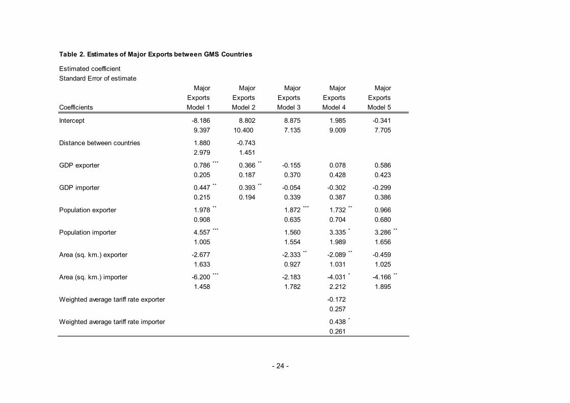
Estimation results For this paper we estimate three basic models: a trade equation (results summarized in Tables 2 and 3), a FDI equation (results summarized in the first two columns of Table 4), and a cross-border road infrastructure equation (results summarized in the last four columns of Table 4). The trade equation was estimated using two alternative definitions of trade: one based on major exports transported via land or river, and the other based on total bilateral trade as reported in the IMF Direction of Trade Statistics database. Our preferred estimation procedure is the random effects estimator for panel data. However, we also estimate trade and FDI equations using single years of data on country pairs to gain additional insight as to how the cross-sectional variation in our estimation models evolved over time. Table 2 presents results of estimates of the value of major exports between GMS countries. Up to 5 commodities (defined at the 4 digit level in the UN Harmonized System of Product Categories) per country pair were selected and summed to generate this measure of trade. The selection of products relied on available (admittedly sketchy) information from customs data for these countries that details or suggests the commodities and goods that are most likely to be transported by road and ferry—where bridges are not available across rivers. Use of disaggregate commodity-specific trade data is preferred to aggregate trade because a larger variety of factors besides cross-border road infrastructure are expected to influence aggregate trade. However, the downside of using the ‘major exports’ is data scarcity and unavoidable subjectivity in the selection of major commodities due to unreliability of customs data at overland points of entry. Table 2 reports results of five estimation models using the major exports variable. The overall goodness of fit of the models is good, with estimated R2 measures ranging between 35.6 percent (Model 1) and 76.2 percent (Model 5). All five models are highly statistically significant, as indicated by the results of the Wald Chi-square test—which reject the null hypothesis that there is no systematic statistical relationship between the models and major exports at a 99 percent confidence level. However, limits on the estimations that use the major exports variables were rather severe due to the relatively small sample size available across GMS countries. These limits made it difficult for panel data models to be estimated and prevented estimation of models that include some variables of interest, so instead, we reverted to a simpler regular Ordinary Least Squares (OLS) regression in Models 3, 4, and 5 reported in Table 2. However, use of the OLS estimator is not supported by our results from the Breusch-Pagan Lagrange Multiplier test. In addition to this specification test, the general sensitivity of these models’ coefficient estimates to changes in the number of right hand side variables that are included suggests that the results of models 3 through 5 are non-robust. Along with the results of the Breusch and Pagan test, this further suggests caution is warranted in interpreting the results of Models 3 to 5. Models 1 and 2 are estimated as random effects panel regressions, and yield coefficient estimates for the basic variables of the gravity model (i.e. GDP, population, and area) that accord with our expectations and with the results generally obtained in gravity model estimates.9 A notable exception to the consistency of our results with previous 9 For example, our estimation results are generally comparable to those reported in Frankel and Romer (1999), Soloaga and Winters (2001), Clarete et al. (2003), Rose (2004), and Yamarik and Ghosh (2005).

- 10 -

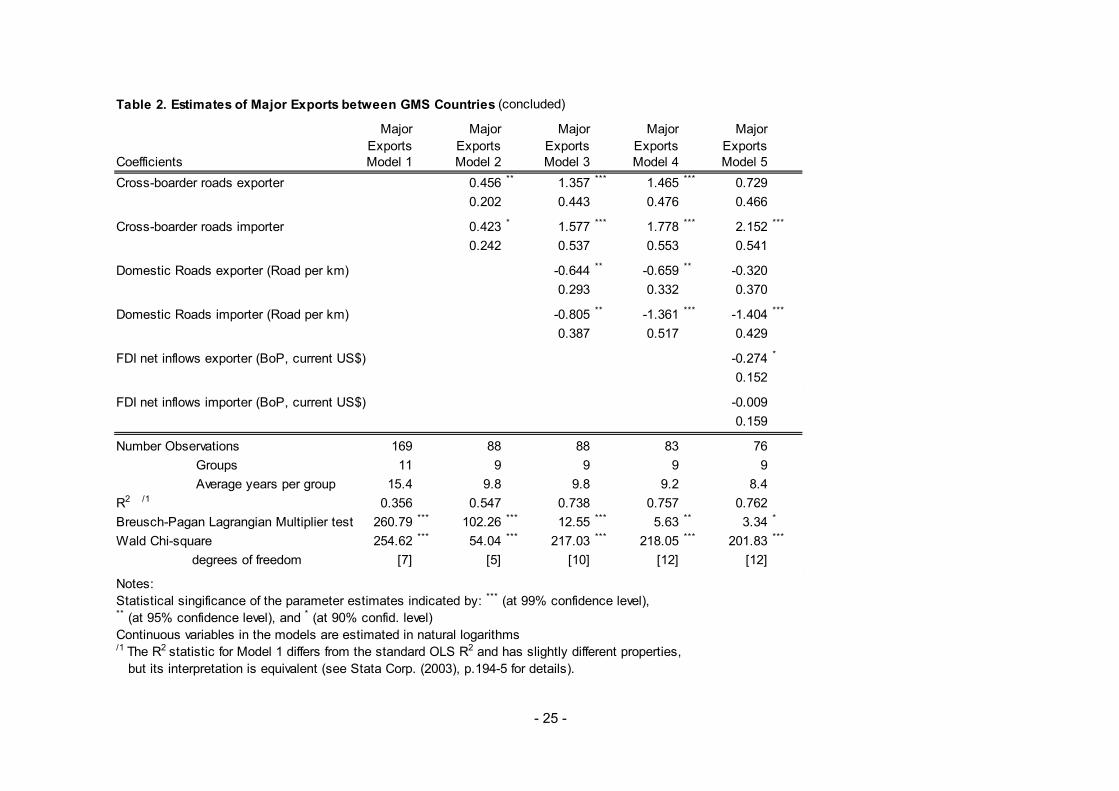
estimates is the non-significant effect that distance is estimated to have on major export flows. This suggests that the distance between capitals may be a poor indicator of the relevant distance in determining overland trade flows between GMS countries, which is understandable since overland trade tends to focus on markets besides the capital city (e.g., regional markets closer to border areas). Unfortunately, limitations of the sample size available prevented estimation of Model 1 in panel form when key variables of interest in addition to the base variables of the gravity equation are added (i.e. the cross-border road measure, an indicator of domestic road infrastructure, and the FDI and tariff measures). Model 2 includes the cross-border infrastructure variables but only the GDP variable from the base variables of the gravity model. Although not detailed in the table, the variation in trade levels observed for pairs of GMS countries was explained largely by changes in the level of trade between countries over time (as opposed to cross-sectional variation across country-pairs).10 A key finding from our estimation Model 2 is that intra-GMS trade via land in major commodities has an elasticity of between 0.42 and 0.46 with respect to cross-border road infrastructure on both sides of the border; which implies that a doubling of the density of roads in border provinces or regions would be expected to induce an average increase in trade in major exports of over 40 percent across the GMS countries. However, when we add a variable measuring domestic road infrastructure to our random effects panel estimates, the statistical significance of cross-border road infrastructure no longer holds, although both variables maintain their positive coefficients. The overall conclusion we reach from the two panel estimates reported in Table 2 (Models 1 and 2) is that trade in major commodities within the GMS is positively influenced by the level of cross-border infrastructure, and that such trade flows are largely driven by economic size of the countries involved and to a lesser but still significant extent by cross-border road infrastructure. To explore the marginal impact of cross-border road infrastructure in addition to the effect of domestic road infrastructure on major exports, we also estimated Models 3 through 5 (also summarized in Table 2). In these models we find that cross-border road infrastructure has an even larger positive and statistically significant association with trade in major exports than that found in our panel estimate (Model 2). Domestic road infrastructure is found to have a negative and statistically significant effect on trade in major exports. One interpretation of this result is that domestic road infrastructure—when separated from roads in frontier areas—mainly promotes the integration of domestic markets within GMS countries and diverts economic activities away from trade in major commodities across GMS countries. Another interpretation is that domestic road infrastructure in GMS complements other infrastructure necessary for ocean-bound trade but not land-bound trade. However, additional information and study is required to assess the validity of this interpretation with confidence. Another coefficient estimate worth noting is the positive and statistically significant effect that importer tariff rates are found to have on major exports, which runs counter to expectations. Table 3 presents estimation results on total exports between GMS countries. Because of the greater number of observations of total exports (rather than major exports via land), we are able to estimate all these models using the preferred random effects panel 10 The time-series component of the estimate is assigned an 83.4 to 88.5 percent weight in the final results reported.

- 11 -

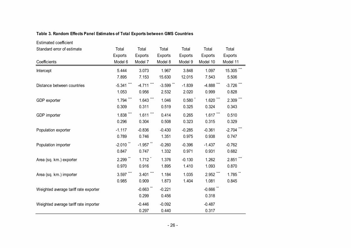
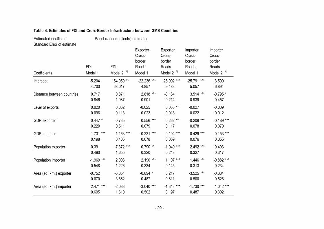
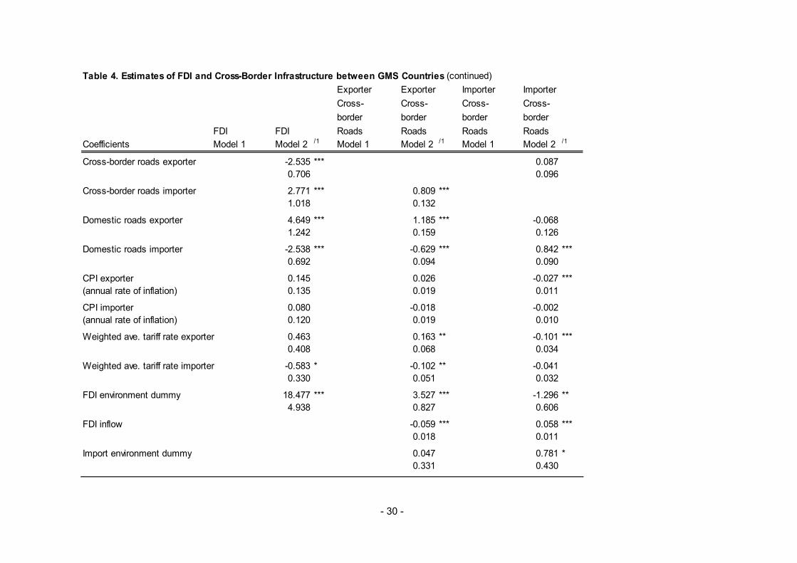
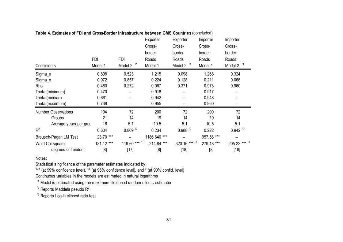
estimator. Use of this estimator is supported by the highly statistically significant results of the Wald Chi-square tests and the results of the Breusch-Pagan Lagrangean Multiplier tests. The models explain between 42.3 and 57.4 percent of the observed variation in aggregate exports between GMS countries. The six variants reported in Table 3 have results that are largely consistent with our expectations and published gravity model results (e.g., negative association between distance and export levels, and the positive association between trading partners’ economic and geographic sizes and their levels of trade). As in earlier studies, the association between trading partner population and total exports is generally negative, although in the majority of cases the association is not statistically significant. The sound performance of Model 6, which includes only the base variables of our gravity model and, the consistency of base variable coefficient estimates across the 6 models reported in Table 3 suggests that the basic gravity model provides a strong base upon which the effect of other variables of interest for trade levels can be usefully judged. Of our particular interest in Table 3 are the estimated coefficients for cross-border and domestic roads, indicators of trade policy and trade environment, and FDI inflows. Models 8 and 9 include an indicator of the trading partners’ cross-border road infrastructure. Such roads have a positive but not statistically significant effect on total trade in Model 8, and have a positive and statistically significant effect on exporter’s total trade in Model 9—which also includes a measure of domestic road infrastructure that also has a positive and statistically significant association with total exports of the exporting economy. This provides limited evidence that cross-border roads favorably influence total exports, although the relationship is clearly weaker than was the case for selected major exports via land. Model 9 also indicates that cross-border and domestic road infrastructure play a complementary role to each other with respect to enhancing aggregate exports among GMS countries, which is contrary to the result we reported in Table 2 in terms of selected major exports via land. Models 7 and 10 in Table 3 show that the average tariff rate has a negative association with total exports, although the association is statistically significant only for the exporting country (while one would typically expect the importing economy’s tariffs to have a greater effect on bilateral trade). This result may be obtained either because tariff barriers are the lesser obstacles to trade than quantitative restrictions and other non-tariff barriers, or because the weighted average tariff rates automatically include all kinds of exemptions as well as “missed” collections by customs authorities, and therefore, understate official tariff rates. In Model 10, our export and import environment dummy variables had signs contrary to our expectations, but neither were statistically significant. This could be because these variables are represented by the extent of administrative time taken by exporters and importers and may have left out other important informal barriers to trade. FDI inflows has no statistically significant association with trade flows, indicating FDI flows may be independent of aggregate trade flows. Lastly, relative real prices across the trading economies—measured by the ratio of the purchasing power parity conversion factor and the official exchange rate—has strong effects on trade with the expected signs. The first two columns of Table 4 present estimation results for FDI inflows. Most of the coefficients show expected signs with statistical significance: e.g., positive association with economic size of the receiving (importer) country; negative association with population size of the exporter country (the larger the economy, the less impetus to invest abroad); and positive association with FDI environment. Both models are

- 12 -

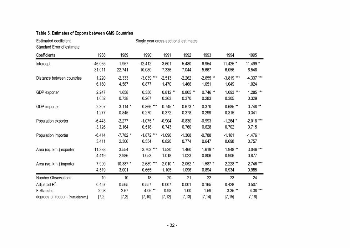
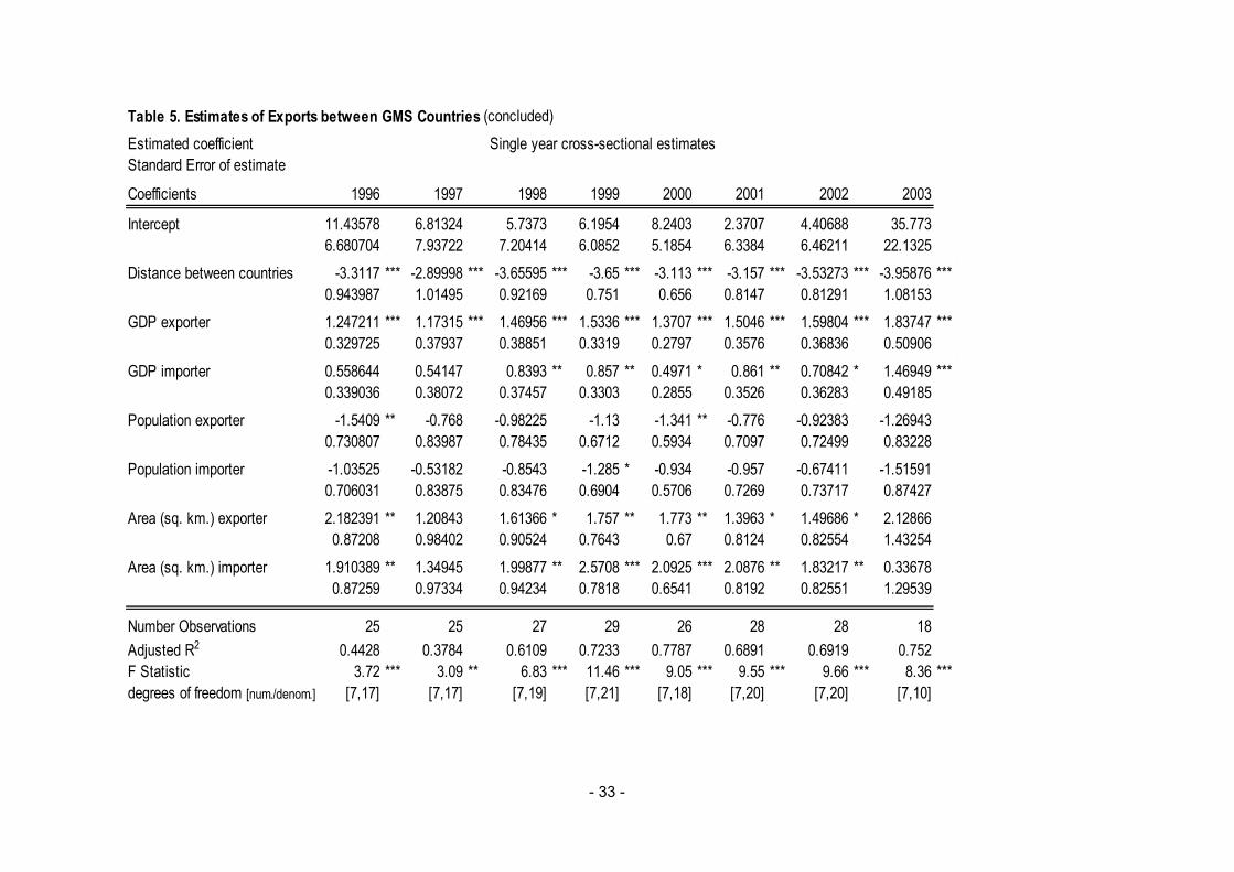
statistically significant overall and explained 60 and 81 percent of the variation in FDI, respectively. The finding that the larger the GDP (and land area) of FDI importer, the higher the level of FDI likely reflects a PRC effect. In model 2, FDI is associated positively with the cross-border infrastructure of the receiving (importer) country but negatively with that of the sending (exporter) country. This may suggest that countries develop cross-border infrastructure in order to entice FDI or that such infrastructure is developed as a condition of FDI. FDI flows are positively and significantly associated with the domestic road infrastructure of the sending country but negatively with that of the receiving country, which is consistent with expectations that capital tends to flow from richer to poorer countries within the GMS and that richer countries tend to have more developed road infrastructures. The last four columns in Table 4 present estimation results on cross-border road infrastructure. By these, we intended to test whether the development of road infrastructure is itself an outcome of the level of trade, FDI and the other standard variables included in a gravity model. Cross-border road infrastructure appears influenced positively by the country’s economic size, both on exporter’s and importer’s sides, presumably due to greater fiscal capacity of larger economies in investing in roads. Similarly cross-border road infrastructure is largely influenced positively by population size. On the other hand, it is largely influenced negatively by the land area, presumably due to the greater difficulty of spreading road network in geographically larger areas. Combined with our results in Table 2, economic and population sizes seem to be the dominant drivers of both trade levels and investment levels in road infrastructure, while cross-border road infrastructure has some identifiable influence on trade levels. It is not clear whether and in which directions the cross-border road infrastructure is associated with FDI inflows. Table 5 summarizes estimation results on total exports in individual years. Our main motive was to investigate stability and trend over time of the relationship between trade level and standard explanatory variables in a gravity model. The associations with distance (negative), economic size (positive), and land area (positive) are fairly stable and consistent with expectations. However, the association with population size is unstable over time, which has been found in previous gravity model studies and in this instance may particularly reflect the massive changes in the People’s Republic of China’s economic relationship with the other GMS countries over time. Table 6 summarizes estimation results on FDI inflows in individual years. One interesting result in the table is the positive and fairly stable association between distance between trading partners and FDI flows. This may suggest that greater distance spurs businesses to move closer to the markets assuming that home-market-oriented FDI is dominant between GMS members – contrary to the production-integration-oriented FDIs that are increasing among the firms in advanced economies. This interpretation is consistent with FDI’s positive and stable association with economic size of the receiving (importer) economy. Conclusions In this paper, we investigated the economic impact of cross-border road infrastructure on trade and FDI flows in the GMS. The theoretical underpinnings of the research drew from recent research in the new economic geography and new trade literatures, while the paper’s estimation approach builds on a basic gravity model framework (following

- 13 -

Limao and Venables, op. cit.). The paper examined three empirical relationships in the context of GMS economies during the past two decades: 1) the association between cross-border infrastructure development and trade between GMS countries, 2) the relationship between cross-border infrastructure development and FDI, and 3) the association between FDI and trade in goods. In addition, the paper measured the marginal effect of cross-border infrastructure on trade and FDI in addition to the general effect of domestic road infrastructure. The study used detailed data on trade flows across GMS countries and measures of road infrastructure and trade policy indicators that were collected for the study (discussed in the Appendix). Nonetheless, sample size constraints associated both with the relatively small number of countries in the GMS and with missing data problems in several GMS countries, represented serious challenges in carrying out econometric estimates for the research. Some particularly notable findings regarding the economic effects of cross-border road infrastructure and other variables we investigate include: (i) The average elasticity of trade in major exports likely to be transported by road

between GMS economies to developments in cross-border road infrastructure is estimated to be over 0.4. This positive effect of cross-border infrastructure on trade in major goods is identified for infrastructure development on both the exporter and importer sides of the borders.

(ii) Cross-border infrastructure is found to have an even larger positive effect on

‘major exports’ when a general measure of domestic road infrastructure is included in the model. In this instance, however, the effect of domestic road infrastructure on trade between GMS countries is actually negative. It is only in the trade equation represented by aggregate trade that a net positive effect of both cross-border and domestic road infrastructure is found.

(iii) Formal trade barriers represented by weighted average tariff rates and trade

environments do not appear to influence trade flows significantly. This may suggest a relatively greater impact of unmeasured non-tariff barriers or that the weighted average tariff rates derived understate official or actual tariff rates.

(iv) Economic and population sizes seem to be the dominant drivers of both trade

and investment in road infrastructure, while cross-border road infrastructure has some identifiable influence on trade levels. Results are inconclusive regarding the significance and direction of cross-border road infrastructure’s effect on FDI inflows.

(v) We find a positive association between FDI inflows and imports (not reported),

suggesting that FDI flows induce further exports from FDI-sending to FDI-receiving economies. This result is consistent with greater flows of raw materials and intermediate inputs needed to run foreign invested operation, anecdotally supported as one outcome of FDI, but may also reflect a loosening of budgets constraints in the face of increased FDI inflows that enable greater imports.

From this study, we conclude that available data suggests the development of cross-border infrastructure in the GMS has played an important role in fostering increased trade within the GMS economies. In addition, empirical findings suggest that

- 14 -

such investments have an effect on trade that is distinct from the effect of domestic road infrastructure in general, and that without investments in cross-border infrastructure domestic road infrastructure could actually lead to reduced intra-GMS trade. This is understandable if one considers the role of domestic roads in linking domestic markets to major seaports, which in turn, connect regional economies to the global economy due to the relatively lower cost of ocean freight. In this light, cross-border road infrastructure becomes an important part of a broader effort to encourage regional integration to benefit GMS member economies that are relatively less endowed with natural seaports. The modeling framework and empirical estimates presented in this paper provide a useful beginning in efforts to estimate some of the key empirical relationships between road infrastructure development, trade, and FDI in the context of the economies of the GMS. Despite difficulties related to the relatively small sample size presented by the GMS economies, the econometric analysis was able to delineate several relationships of interest. But without significant enhancements to the analytical dataset, we must express some skepticism regarding the promise of additional econometric research that makes use of the gravity model approach for the group of countries. Accordingly, extensions of this research could focus principally on considering applied simulation models to generate quantitative estimates of the aggregate economic impact of increases in trade attributable to cross-border road infrastructure development. One relatively simple extension that could help illustrate the implications of the paper’s findings would be to take estimation parameters as given and forecast aggregate trade and GDP effects of future infrastructure investment. However, a more nuanced—and useful—simulation model would require better understanding of the various causal channels through which increased trade translates into economic benefits (i.e. including direct trade-related service outputs and other economic activities indirectly induced through forward and backward linkages). While multi-sector general equilibrium models would be theoretically superior in pursuing estimation of these impacts by country, a useful initial step might be to begin with fixed-coefficient application for estimating these impacts, using input-output tables and social accounting matrices (SAM). The analysis would begin with countries where these existing analytical tools are available, such as Thailand and Viet Nam. Also, some case-specific estimation for benefit-cost incidence can be attempted on, for example, North-South Economic Corridor that involves Thailand, Lao PDR and the People’s Republic of China.11 Analysis of the social and environmental effects of the cross-border road infrastructure is clearly crucial as well. Integrating findings by many researchers regarding social and environmental effects, which have tended to be mainly qualitative, and the findings of econometric analysis of infrastructure development and trade and FDI linkages represents a particularly daunting but important extension of this research.

11 An unpublished report by the authors based on field research carried out along the North-South Economic Corridor in August-September of 2005 includes a discussion of possible distribution analysis of the impact of cross-border road infrastructure that is based on standard methodology for project economic analysis. This discussion notes a number of shortcomings in the standard methodology in terms of its capacity to capture relevant project externalities—including those associated with cross-border infrastructure.

- 15 -

References

Adhikari, R. and J. Weiss. 1999. “Economic Analysis of Subregional Projects”. EDRC Methodology Series No.1. Asian Development Bank. March 1999. Manila.

Clarete, R., C. Edmonds, and J.S. Wallack. 2003. “Asian regionalism and its effects on trade in the 1980s and 1990s” Journal of Asian Economics 14: 91-131.

Dollar, D., and A. Kraay. 2004. “Trade, Growth, and Poverty.” The Economic Journal 114(493): 22-49.

Edwards, S. 1993 “Openness, Trade Liberalization, and Growth in Developing Countries.” Journal of Economic Literature 31(3): 1358-93.

Ferroni, M. 2002. “Regional Public Goods in Official Development Assistance”, in M. Ferroni and A. Mody, eds. International Public Goods: Incentives, Measurement, and Financing. Dordecht, NL: Kluwer Academic Publishers.

Frankel, J., and D. Romer. 1999. “Does Trade Cause Growth?” American Economic Review 89(3): 379-399.

Fujimura, M. 2004. “Cross-Border Transport Infrastructure, Regional Integration and Development” ADBI Discussion Paper No.16.

Fukao, K., H. Ishido and K. Ito. 2003. “Vertical Intra-industry Trade and Foreign Direct Investment in East Asia” Journal of the Japanese and International Economies 17(4): 468-506.

Green, W. 2003. Econometric Analysis (Fifth Edition), New Jersey: Prentice Hall Publishers.

Harrison, A. 1996. “Openness and Growth: A Time-Series, Cross-Country Analysis for Developing Countries.” Journal of Development Economics 48(2):419-47.

Lee, H., D. Roland-Holst, and D. van der Mensbrugghe. 2004. “China's Emergence in East Asia under Alternative Trading Arrangements.” Journal of Asian Economics 15(4): 697-712.

Limao, N., and A.J. Venables. 2001. “Infrastructure, Geographical Disadvantage, Transport Costs and Trade.” World Bank Economic Review 15: 451-479.

Markusen, J.R. and A.J. Venables. 2000. “The Theory of Endowment, Intra-Industry and Multi-National Trade.” Journal of International Economics 52: 209-234.

McLaren, J. 1996. “Size, Sunk Costs, and Judge Bowker’s Objection to Free Trade.” American Economic Review 87(3): 400-420.

Oldfield, D.D. 2004. “Border Trade Facilitation and Logistics Development in the GMS: Component I – Review of Logistics Development in GMS”, Asia Policy Research Co. Ltd., a report submitted to United Nations Economic and Social Committee for Asia-Pacific (UNESCAP).

- 16 -

Radelet, S. and J. Sachs, 1998. “Shipping Costs, Manufactured Exports, and Economic Growth”, paper presented at American Economic Association meeting, Harvard University.

Redding, S. and A.J. Venables. 2004. “Economic Geography and International Inequality” Journal of International Economics 62: 53-82.

Rose, A.K. 2004. “Do We Really Know That The WTO Increases Trade?” American Economic Review, 94: 98-114.

Soloaga, I., and A. Winters, 2001. “Regionalism in the Nineties: What Effect on Trade?” North American Journal of Economics and Finance 12:1-29.

Stata Corp. (2003) Stata Cross-Sectional Time-Series Reference Manual (Release 8), College Station, Texas: Stata Press.

Urata, S. 2001. “Emergence of an FDI-Trade Nexus and Economic Growth in East Asia” in J. Stiglitz and S. Yusuf (eds.), Rethinking the East Asian Miracle (Washington DC: World Bank and Oxford University Press).

World Bank. Doing Business database. Available on-line at: Hhttp://www.doingbusiness.org/.H

Yamarik, S. and S. Ghosh. 2005. “A Sensitivity Analysis of The Gravity Model”. The International Trade Journal 19: 83-126.

- 17 -

Appendix: Notes on Data for Key Variables

(1) Road infrastructure Availability, level of details, and types of data on road infrastructure vary among GMS members, necessitating some procedure of making the data consistent and comparable across the GMS members. Therefore, our quantitative analysis used road density for GMS members where road inventory data are available and density of freight carriage for those where road inventory data are not available but administrative data on freights are available. For Cambodia, there are no geographically disaggregated data on road inventory. 1995 data provided by the Committee for Development of Cambodia (CDC) was the only disaggregated data by province made available to the authors. This information was extrapolated by the available aggregate road length figures for the subsequent years in calculating road density by province. For Lao PDR, data on road inventory and density by province were provided directly by the Department of Roads, Ministry of Communication, Transport, Post and Construction, upon the request of the authors. For Thailand, road inventory data from Department of Highways, Ministry of Transport are disaggregated only by the route of national highways which run through multiple provinces. These data are adjusted by the estimated provincial shares based on the GIS-based “Road Inventory of ASEAN Highways” developed by UNESCAP in calculating road density by province. For Myanmar and Viet Nam, there exist no official data on road length. Instead, various administrative data included in the transport section of the statistical yearbooks were combined to calculate the density of freight carriage by state/province. For Yunnan Province, road density by region was calculated from the road inventory data available in the transport section of the provincial statistical yearbooks. Distinction between cross-border and domestic road infrastructure was made for each pair of GMS members based on the location of international crossing points as presented in Table A1. For example, Cambodia’s cross-border and domestic road infrastructure with respect to Lao PDR is represented by road density of Stung Treng Province and that of all the other provinces (which do not share border with the other GMS members), respectively. Likewise, Lao PDR’s cross-border and domestic road infrastructure with respect to Cambodia is represented by road density in Champassack Province and all the other provinces (which do not share a border with the other GMS members), respectively. Where there is more than one province with shared borders with a neighbor country, the corresponding cross-border road infrastructure is represented by the average of the road density in such provinces. Likewise, domestic road infrastructure is represented by the average of the road density in the remaining provinces. “Local border points” as opposed to “international cross-border points”, as often referred to by public institutions in GMS, are the borders where only the residents in immediately neighboring provinces/states can cross borders and trade freely. While some of these borders might carry noticeable but unrecorded trade volumes, their traffic would mainly be limited to those immediate neighboring provinces/states and therefore, of limited economic impact on the subregion as a whole. Because the focus of this paper is on the impact of road infrastructure on the entire GMS economies, it makes sense to focus on the international crossing points and leave out local border points. This treatment also seems to be a convenient way of making quantitative analysis consistent between the road infrastructure data and the officially recorded trade data that are the only available data in any reasonable time series.

- 18 -

Table A1: International crossing points in GMS used in distinction between

cross-border and domestic road infrastructure GMS member A GMS member B

Borders between A/B

Name of border city/town

Name of border province/state

Name of border city/town

Name of border province/state

Cambodia/Lao PDR Trapeangkreal Stung Treng Province Khinak Champassack Province

Cambodia/Thailand Poipet Bantreay Meanchey Province Arayaprathet Sa Kaeo Province Cham Yeam Koh Kong Province Hat Lek Trat Province

Cambodia/Viet Nam Bavet Xvay Rieng Province Moc bai Tay Ninh Province

Lao PDR/Thailand Huoayxay Bokeo Province Chiang Khong Chiang Rai Province Thanaleng Vientiane Municipality Nong Khai Nong Khai Province Thakhek Khammouan Province Nakhon Phanom Nakohn Panom Province Savannakhet Savannakhet Province Mukdahan Mukdahan Province

Lao PDR/Viet Nam Nam Phao Borikhamxay Province Cau Treo Ha Tinh Province Densavanh Savannakhet Province Lao Bao Quang Tri Province

Lao PDR/Yunnan Boten Luangnamtha Province Mengla Xishuanbanna Region Myanmar/Thailand Myawadi Kayin State Mae Sot Tak Province

Tachilek Shan State Mae Sai Chiang Rai Province Myanmar/Yunnan Mongla Shan State Daluo Xishuanbanna Region

Muse Shan State Ruili Baoshan Region Viet Nam/Yunnan Lao Cai Lao Cai Province Hekou Wenshan Region

(Source) UNESCAP Asian Highway Database 2004; regional maps and atlas (2) Distance Data on distance between each pair of GMS members were taken from Oldfield (2004) as summarized in Table A2.

Table A2: Distance between major markets in GMS Distance between Major markets involved km Cambodia - Lao PDR Phnom Penh - Vientiane 753 Cambodia - Myanmar Phonm Penh - Yangon 1101 Cambodia - Thailand Phnom Penh - Bangkok 530 Cambodia - Viet Nam Phnom Penh - Ho Chi Minh City 217 Cambodia - Yunnan Phnom Penh - Kunming 1519 Lao PDR - Myanmar Vientiane - Yangon 695 Lao PDR - Thailand Vientiane - Bangkok 521 Lao PDR - Viet Nam Vientiane - Hanoi 482 Lao PDR - Yunnan Vientiane - Kunming 789 Myanmar - Thailand Yangon - Bangkok 575 Myanmar - Viet Nam Yangon - Hanoi 1123 Myanmar - Yunnan Yangon - Kunming 1142 Thailand - Viet Nam Bangkok - Ho Chi Minh City 754 Thailand - Yunnan Bangkok - Kunming 1280 Viet Nam - Yunnan Hanoi - Kunming 555

- 19 -

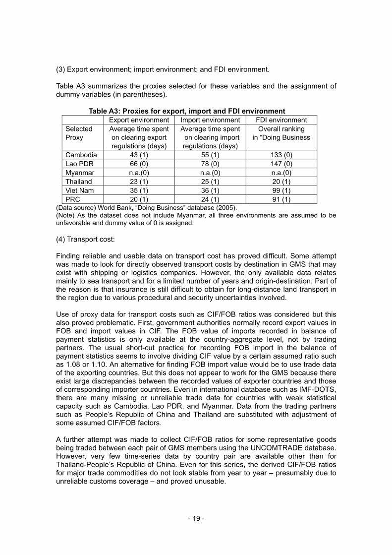
(3) Export environment; import environment; and FDI environment. Table A3 summarizes the proxies selected for these variables and the assignment of dummy variables (in parentheses). Table A3: Proxies for export, import and FDI environment

Export environment Import environment FDI environment Selected Proxy

Average time spent on clearing export regulations (days)

Average time spent on clearing import regulations (days)

Overall ranking in “Doing Business

Cambodia 43 (1) 55 (1) 133 (0) Lao PDR 66 (0) 78 (0) 147 (0) Myanmar n.a.(0) n.a.(0) n.a.(0) Thailand 23 (1) 25 (1) 20 (1) Viet Nam 35 (1) 36 (1) 99 (1) PRC 20 (1) 24 (1) 91 (1)

(Data source) World Bank, “Doing Business” database (2005). (Note) As the dataset does not include Myanmar, all three environments are assumed to be unfavorable and dummy value of 0 is assigned. (4) Transport cost: Finding reliable and usable data on transport cost has proved difficult. Some attempt was made to look for directly observed transport costs by destination in GMS that may exist with shipping or logistics companies. However, the only available data relates mainly to sea transport and for a limited number of years and origin-destination. Part of the reason is that insurance is still difficult to obtain for long-distance land transport in the region due to various procedural and security uncertainties involved. Use of proxy data for transport costs such as CIF/FOB ratios was considered but this also proved problematic. First, government authorities normally record export values in FOB and import values in CIF. The FOB value of imports recorded in balance of payment statistics is only available at the country-aggregate level, not by trading partners. The usual short-cut practice for recording FOB import in the balance of payment statistics seems to involve dividing CIF value by a certain assumed ratio such as 1.08 or 1.10. An alternative for finding FOB import value would be to use trade data of the exporting countries. But this does not appear to work for the GMS because there exist large discrepancies between the recorded values of exporter countries and those of corresponding importer countries. Even in international database such as IMF-DOTS, there are many missing or unreliable trade data for countries with weak statistical capacity such as Cambodia, Lao PDR, and Myanmar. Data from the trading partners such as People’s Republic of China and Thailand are substituted with adjustment of some assumed CIF/FOB factors. A further attempt was made to collect CIF/FOB ratios for some representative goods being traded between each pair of GMS members using the UNCOMTRADE database. However, very few time-series data by country pair are available other than for Thailand-People’s Republic of China. Even for this series, the derived CIF/FOB ratios for major trade commodities do not look stable from year to year – presumably due to unreliable customs coverage – and proved unusable.

- 20 -

Table 1. Descriptive statistics from the dataset used in estimates

Variable Units Mean Std. Dev. Minimum MaximumSource(s) and notes

Country-pair n.a. overall N 690 353.5 170.6 102 605identification code between n 30

within T 23

Year n.a. overall N 690 1992 6.6 1981 2003between n 30within T 23

Trade and tarde policiesCountry 1's exports mil. current US$ overall N 475 112.75 288.84 0.00 2853.60 1,2,3to country 2 between n 29

within T-bar 16.4

Major exports from mil. current US$ overall N 171 74.71 125.43 0.04 845.01 4,5country 1 to 2 between n 11

within T 15.5

Country 1's imports mil. current US$ overall N 442 116.59 261.21 0.00 2464.08 1,2,3from country 2 between n 27

within T-bar 16.4

Weighted average expressed in overall N 525 0.158 0.174 0.023 1.050 6,7tariff rate fraction between n 30

within T-bar 17.5

Export environment dummy (0/1) overall N 690 0.6667 0.471747 0 1 8between n 30within T 23

Import environment dummy (0/1) overall N 690 0.6667 0.471747 0 1 8between n 30within T 23

Number observations

- 21 -

Table 1. Descriptive statistics from the dataset used in estimates (continued)


FDI and FDI policiesCountry 1's FDI inflow mil. current US$ overall N 231 7.0569 13.677 -9.020 97.390 9,10from country 2 between n 21

within T-bar 11

Outward FDI mil. current US$ overall N 375 6,550 13,300 0 47,200 11between n 30within T-bar 12.5

Net FDI inflow mil current US$ overall N 570 4,830 12,100 -1.6 53,500 11between n 30within T 19

FDI environment dummy (0/1) overall N 690 0.5000 0.500 0 1 12between n 30within T 23

Gross FDI as % of GDP % overall N 370 3.415 2.398 0.000 9.713 11between n 25within T-bar 14.8

Distance and roadsDistance between kilometer overall N 690 802.4 344.4 217.0 1519.0 13,14,15country 1 and 2 between n 30

within T 23

Country 1's road km/km2 or overall N 223 0.114 0.123 0.002 0.567 16,17infrastructure in ton-km/km2 between n 19regions bordering within T-bar 11.7country 2

Country 1's road km/km2 or overall N 370 0.813 1.247 0.007 4.047 16,17infrastructure in ton-km/km2 between n 30interior regions within T-bar 12.3

Number observations

- 22 -

Table 1. Descriptive statistics from the dataset used in estimates (continued)


Paved roads % of total overall N 230 34.596 33.300 7.500 98.500 11between n 25within T 9.2

Road network total km overall N 300 334,152 550293 12323 1765222 11between n 30within T 10

Country economic characteristicsGDP bil. current US$ overall N 570 26.05 42.11 0.60 181.50 6,18

between n 30within T-bar 19

GDP deflator % overall N 510 26.55 66.71 -4.04 411.04 11between n 30within T-bar 17

Current exchange rate LCU per US$ overall N 540 2505.39 4346.14 2.94 15509.58 11annual average between n 30

within T-bar 18

Consumer price index % overall N 435 13.735 19.765 -1.710 128.419 11between n 30within T-bar 14.5

Total debt service mil. current US$ overall N 570 4,120 7,450 0 37,100 11between n 30within T 19

PPP conversion factor ratio to overall N 415 0.273 0.117 0.099 0.795 11official exch. between n 25exch. rate within T-bar 16.6

Real interest rate % overall N 440 2.641 11.589 -41.715 20.328 11between n 30within T-bar 14.7

Number observations

- 23 -

Table 1. Descriptive statistics from the dataset used (concluded)

Variable Unit Mean Std. Dev. Minimum Maximum Source(s) and notes

Other country characteristics Total population number (mil.) overall N 570 229.0 429.00 3.62 1290.00 11 between 30

within T 19Land area s quare km (thou.) overall N 570 1,871 3,341 177 9,327 11

between n 30within T 19

Arable land area h ectares (thou.) overall N 540 27,200 45,000 792 144,000 11between n 30within T 18

Notes: 1) IMF Direction of Trade Statistics (2005).

12) World Bank Doing Business data (various years). See Appendix for the procedure of producing dummy variable.13) Statistical yearbooks for Myanmar, Viet Nam and Yunnan (various

)

7) WATR is calculated by dividing customs revenue by imports. Weighting of trade items by value is done automatically by this procedure.8) World Bank Doing Business data (various years). See Appendix for the procedure of producing dummy variable.9) Reports of the: Cambodian Investment Board for Cambodia, Department of Domestic and Foreign Investment for Lao PDR, and Bank of Thailand (BOP basis) for Th il d10) Data for Cambodia, Lao PDR, Myanmar, and Viet Nam are approved amounts by investment approving authorities, adjusted by estimated average implementation

i dsmoothed by 5-year moving average. Data for Thailand are “net FDI inflows” recorded by the Bank of Thailand. Data for Yunnan Province are the “actually utilized” amountrecorded in the provincial statistical yearbooks. Estimated investments in energy sector are excluded.

4) UNCOMTRADE data from Statistics Canada's Trade Analayzer database (2005).5) Up to 5 commodities (HS 4 digits) were selected relying on available information on border trades in the subregion.

14) Oldfield (2004).15) Distance between capital cities was chosen, except for cases of Cambodia-Viet Nam and Thailand-Viet Nam where Ho Chi Minh City is used in preference to Hanoi since itrepresents largest Vietnamese city near the other two countries' capitals.16) Separate sources were used for the countries. See Appendix for details.17) Different measures of cross border road infrastructure are used depending upon data availability: and for Cambodia, Lao PDR, Thailand and Yunnan--km/km2 (road density); fMyanmer and Viet Nam--ton-km/km2 (freight carriage density).18) Country 2's GDP is also defined but only for the purpose of pairing. This is true for all variables ending in "1".

2) Yunnan statistical yearbooks (various years).3) Approximate adjustments were made to exclude river- and sea-born trade and gas trade. Yunnan exports are specific to Yunnan Province.

6) ADB Key Indicators and statistical yearbooks of GMS members (various years).

11) World Bank, World Development Indicators (2005).

Number observations

n

- 24 -

Table 2. Estimates of Major Exports between GMS Countries

Estimated coefficientStandard Error of estimate

Major Major Major Major MajorExports Exports Exports Exports Exports

Coefficients Model 1 Model 2 Model 3 Model 4 Model 5

Intercept -8.186 8.802 8.875 1.985 -0.3419.397 10.400 7.135 9.009 7.705

Distance between countries 1.880 -0.7432.979 1.451

GDP exporter 0.786 *** 0.366 ** -0.155 0.078 0.5860.205 0.187 0.370 0.428 0.423

GDP importer 0.447 ** 0.393 ** -0.054 -0.302 -0.2990.215 0.194 0.339 0.387 0.386

Population exporter 1.978 ** 1.872 *** 1.732 ** 0.9660.908 0.635 0.704 0.680

Population importer 4.557 *** 1.560 3.335 * 3.286 **

1.005 1.554 1.989 1.656

Area (sq. km.) exporter -2.677 -2.333 ** -2.089 ** -0.4591.633 0.927 1.031 1.025

Area (sq. km.) importer -6.200 *** -2.183 -4.031 * -4.166 **

1.458 1.782 2.212 1.895

Weighted average tariff rate exporter -0.1720.257

Weighted average tariff rate importer 0.438 *

0.261

- 25 -

Table 2. Estimates of Major Exports between GMS Countries (concluded)

Major Major Major Major MajorExports Exports Exports Exports Exports

Coefficients Model 1 Model 2 Model 3 Model 4 Model 5Cross-boarder roads exporter 0.456 ** 1.357 *** 1.465 *** 0.729

0.202 0.443 0.476 0.466

Cross-boarder roads importer 0.423 * 1.577 *** 1.778 *** 2.152 ***

0.242 0.537 0.553 0.541

Domestic Roads exporter (Road per km) -0.644 ** -0.659 ** -0.3200.293 0.332 0.370

Domestic Roads importer (Road per km) -0.805 ** -1.361 *** -1.404 ***

0.387 0.517 0.429

FDI net inflows exporter (BoP, current US$) -0.274 *

0.152

FDI net inflows importer (BoP, current US$) -0.0090.159

Number Observations 169 88 88 83 76 Groups 11 9 9 9 9 Average years per group 15.4 9.8 9.8 9.2 8.4R2 /1 0.356 0.547 0.738 0.757 0.762Breusch-Pagan Lagrangian Multiplier test 260.79 *** 102.26 *** 12.55 *** 5.63 ** 3.34 *

Wald Chi-square 254.62 *** 54.04 *** 217.03 *** 218.05 *** 201.83 ***

degrees of freedom [7] [5] [10] [12] [12]

Notes:Statistical singificance of the parameter estimates indicated by: *** (at 99% confidence level), ** (at 95% confidence level), and * (at 90% confid. level)Continuous variables in the models are estimated in natural logarithms/1 The R2 statistic for Model 1 differs from the standard OLS R2 and has slightly different properties, but its interpretation is equivalent (see Stata Corp. (2003), p.194-5 for details).

- 26 -

Table 3. Random Effects Panel Estimates of Total Exports between GMS Countries

Estimated coefficientStandard error of estimate Total Total Total Total Total Total

Exports Exports Exports Exports Exports ExportsCoefficients Model 6 Model 7 Model 8 Model 9 Model 10 Model 11

Intercept 5.444 3.073 1.967 3.848 1.097 15.305 ***

7.895 7.153 15.630 12.015 7.543 5.506

Distance between countries -5.341 *** -4.711 *** -3.599 ** -1.839 -4.888 *** -3.726 ***

1.053 0.956 2.532 2.020 0.999 0.828

GDP exporter 1.794 *** 1.643 *** 1.046 0.580 * 1.620 *** 2.309 ***

0.309 0.311 0.519 0.325 0.324 0.343

GDP importer 1.838 *** 1.611 *** 0.414 0.265 1.617 *** 0.5100.296 0.304 0.508 0.323 0.315 0.329

Population exporter -1.117 -0.836 -0.430 -0.285 -0.361 -2.704 ***

0.789 0.746 1.351 0.975 0.938 0.747

Population importer -2.010 ** -1.957 ** -0.260 -0.396 -1.437 -0.7620.847 0.747 1.332 0.971 0.931 0.682

Area (sq. km.) exporter 2.299 ** 1.712 * 1.376 -0.130 1.262 2.851 ***

0.970 0.916 1.895 1.410 1.093 0.870

Area (sq. km.) importer 3.597 *** 3.401 *** 1.184 1.035 2.952 *** 1.785 **

0.985 0.909 1.873 1.404 1.081 0.845

Weighted average tariff rate exporter -0.663 ** -0.221 -0.666 **

0.299 0.456 0.318

Weighted average tariff rate importer -0.446 -0.092 -0.4870.297 0.440 0.317

- 27 -

Table 3. Random Effects Panel Estimates of Total Exports between GMS Countries (continued)Estimated coefficientStandard error of estimate Total Total Total Total Total Total


Cross-boarder roads exporter 0.065 0.474 *

0.472 0.287

Cross-boarder roads importer 0.452 -0.0500.456 0.285

Domestic Roads exporter (Road per km) 0.759 ***

0.296

Domestic Roads importer (Road per km) 0.2300.317

Export environment dummy (EXPe1_d1) -1.1551.363

Import environment dummy (EXPe2_d1) -1.3011.339

FDI net inflows exporter (BoP, current US$) 0.1860.174

FDI net inflows importer (BoP, current US$) 0.0410.163

- 28 -

Table 3. Random Effects Panel Estimates of Total Exports between GMS Countries (concluded)Estimated coefficientStandard error of estimate Total Total Total Total Total Total


PPP exporter -2.430 ***

0.754

PPP importer 2.354 ***

0.677

Sigma_u 2.990 1.826 2.275 1.850 1.907 1.243Sigma_e 2.489 2.525 1.782 0.603 2.525 1.390Rho 0.416 0.343 0.620 0.904 0.363 0.444Theta (minimum) 0.564 0.376 0.669 0.690 0.393 0.512Theta (median) 0.698 0.629 0.747 0.856 0.643 0.681Theta (maximum) 0.738 0.690 0.770 0.878 0.702 0.745

Number Observations 392 326 156 89 326 227 Groups 29 29 18 18 29 20 Average years per group 13.5 11.2 8.7 4.9 11.2 11.4R2 0.491 0.480 0.474 0.423 0.493 0.574Breusch-Pagan Lagrangian Multiplier test 77.62 *** 45.95 *** 41.16 *** 35.27 *** 43.87 *** 32.28 ***

Wald Chi-square 147.67 *** 153.17 *** 25.46 *** 33.35 *** 151.17 *** 140.44 ***

degrees of freedom [7] [9] [11] [11] [11] [11]

Notes:Statistical singificance of the parameter estimates indicated by: *** (at 99% confidence level),** (at 95% confidence level), and * (at 90% confid. level)Continuous variables in the models are estimated in natural logarithms/1 The R2 statistic for Model 1 differs from the standard OLS R2 and has slightly different properties, but its interpretation is equivalent (see Stata Corp. (2003), p.194-5 for details).

- 29 -

Table 4. Estimates of FDI and Cross-Border Infrastructure between GMS Countries

Estimated coefficient Panel (random effects) estimates Standard Error of estimate

Exporter Exporter Importer ImporterCross- Cross- Cross- Cross-border border border border

FDI FDI Roads Roads Roads RoadsCoefficients Model 1 Model 2 /1 Model 1 Model 2 /1 Model 1 Model 2 /1

Intercept -5.204 154.059 ** -22.236 *** 28.992 *** -25.791 *** 3.5994.700 63.017 4.857 9.483 5.057 6.894

Distance between countries 0.717 0.871 2.818 *** -0.184 3.514 *** -0.795 *0.846 1.087 0.901 0.214 0.939 0.457

Level of exports 0.020 0.062 -0.025 0.038 ** -0.027 -0.0090.096 0.118 0.023 0.018 0.022 0.012

GDP exporter 0.447 * 0.735 0.556 *** 0.262 ** -0.209 *** -0.189 ***0.229 0.511 0.079 0.117 0.078 0.070

GDP importer 1.731 *** 1.163 *** -0.221 *** -0.194 *** 0.429 *** 0.153 ***0.198 0.405 0.078 0.059 0.076 0.055

Population exporter 0.391 -7.372 *** 0.790 ** -1.949 *** 2.492 *** 0.4030.490 1.655 0.320 0.243 0.327 0.317

Population importer -1.969 *** 2.003 2.190 *** 1.107 *** 1.446 *** -0.882 ***0.548 1.226 0.334 0.145 0.313 0.234

Area (sq. km.) exporter -0.752 -3.851 -0.894 * 0.217 -3.525 *** -0.3340.670 3.852 0.487 0.611 0.500 0.526

Area (sq. km.) importer 2.471 *** -2.088 -3.040 *** -1.343 *** -1.730 *** 1.042 ***0.695 1.610 0.502 0.197 0.487 0.302

- 30 -

Table 4. Estimates of FDI and Cross-Border Infrastructure between GMS Countries (continued)Exporter Exporter Importer ImporterCross- Cross- Cross- Cross-border border border border


Cross-border roads exporter -2.535 *** 0.0870.706 0.096

Cross-border roads importer 2.771 *** 0.809 ***1.018 0.132

Domestic roads exporter 4.649 *** 1.185 *** -0.0681.242 0.159 0.126

Domestic roads importer -2.538 *** -0.629 *** 0.842 ***0.692 0.094 0.090

CPI exporter 0.145 0.026 -0.027 ***(annual rate of inflation) 0.135 0.019 0.011

CPI importer 0.080 -0.018 -0.002(annual rate of inflation) 0.120 0.019 0.010

Weighted ave. tariff rate exporter 0.463 0.163 ** -0.101 ***0.408 0.068 0.034

Weighted ave. tariff rate importer -0.583 * -0.102 ** -0.0410.330 0.051 0.032

FDI environment dummy 18.477 *** 3.527 *** -1.296 **4.938 0.827 0.606

FDI inflow -0.059 *** 0.058 ***0.018 0.011

Import environment dummy 0.047 0.781 *0.331 0.430

- 31 -

Table 4. Estimates of FDI and Cross-Border Infrastructure between GMS Countries (concluded)Exporter Exporter Importer ImporterCross- Cross- Cross- Cross-border border border border


Sigma_u 0.898 0.523 1.215 0.098 1.268 0.324Sigma_e 0.972 0.857 0.224 0.128 0.211 0.066Rho 0.460 0.272 0.967 0.371 0.973 0.960Theta (minimum) 0.470 -- 0.918 -- 0.917 -- Theta (median) 0.661 -- 0.942 -- 0.948 -- Theta (maximum) 0.739 -- 0.955 -- 0.960 --

Number Observations 194 72 200 72 200 72 Groups 21 14 19 14 19 14 Average years per grou 16 5.1 10.5 5.1 10.5 5.1R2 0.604 0.809 /2 0.234 0.988 /2 0.222 0.942 /2

Breusch-Pagan LM Test 23.70 *** -- 1186.640 *** -- 957.56 *** -- Wald Chi-square 131.12 *** 119.60 *** /3 214.84 *** 320.16 *** /3 279.18 *** 205.22 *** /3

degrees of freedom [8] [17] [8] [18] [8] [18]

Notes:Statistical singificance of the parameter estimates indicated by: *** (at 99% confidence level), ** (at 95% confidence level), and * (at 90% confid. level)Continuous variables in the models are estimated in natural logarithms /1 Model is estimated using the maximum likelihood random effects estimator /2 Reports Maddela pseudo R2

/3 Reports Log-likelihood ratio test

- 32 -

Table 5. Estimates of Exports between GMS CountriesEstimated coefficient Single year cross-sectional estimatesStandard Error of estimate

Coefficients 1988 1989 1990 1991 1992 1993 1994 1995

Intercept -46.065 -1.957 -12.412 3.601 5.480 6.954 11.425 * 11.499 *31.011 22.741 10.080 7.336 7.044 5.667 6.056 6.548

Distance between countries 1.220 -2.333 -3.039 *** -2.513 -2.262 -2.655 ** -3.819 *** -4.337 ***6.160 4.587 0.877 1.470 1.466 1.051 1.049 1.024

GDP exporter 2.247 1.658 0.356 0.812 ** 0.805 ** 0.746 ** 1.093 *** 1.285 ***1.052 0.738 0.267 0.363 0.370 0.283 0.305 0.329

GDP importer 2.307 3.114 * 0.866 *** 0.745 * 0.673 * 0.370 0.685 ** 0.748 **1.277 0.845 0.270 0.372 0.378 0.299 0.315 0.341

Population exporter -6.443 -2.277 -1.075 * -0.904 -0.830 -0.993 -1.264 * -2.018 ***3.126 2.164 0.518 0.743 0.760 0.628 0.702 0.715

Population importer -6.414 -7.782 * -1.872 *** -1.096 -1.308 -0.788 -1.161 -1.476 *3.411 2.306 0.554 0.820 0.774 0.647 0.698 0.757

Area (sq. km.) exporter 11.338 3.554 3.703 *** 1.520 1.460 1.619 * 1.948 ** 3.046 ***4.419 2.986 1.053 1.018 1.023 0.806 0.906 0.877

Area (sq. km.) importer 7.990 10.387 * 2.689 *** 2.010 * 2.052 * 1.587 * 2.228 ** 2.746 ***4.519 3.001 0.665 1.105 1.096 0.894 0.934 0.985

Number Observations 10 10 18 20 21 22 23 24Adjusted R2 0.457 0.565 0.557 -0.007 -0.001 0.165 0.428 0.507F Statistic 2.08 2.67 4.06 ** 0.98 1.00 1.59 3.35 ** 4.38 ***degrees of freedom [num./denom.] [7,2] [7,2] [7,10] [7,12] [7,13] [7,14] [7,15] [7,16]

- 33 -

Table 5. Estimates of Exports between GMS Countries (concluded)

Estimated coefficient Single year cross-sectional estimatesStandard Error of estimate

Coefficients 1996 1997 1998 1999 2000 2001 2002 2003

Intercept 11.43578 6.81324 5.7373 6.1954 8.2403 2.3707 4.40688 35.7736.680704 7.93722 7.20414 6.0852 5.1854 6.3384 6.46211 22.1325

Distance between countries -3.3117 *** -2.89998 *** -3.65595 *** -3.65 *** -3.113 *** -3.157 *** -3.53273 *** -3.95876 ***0.943987 1.01495 0.92169 0.751 0.656 0.8147 0.81291 1.08153

GDP exporter 1.247211 *** 1.17315 *** 1.46956 *** 1.5336 *** 1.3707 *** 1.5046 *** 1.59804 *** 1.83747 ***0.329725 0.37937 0.38851 0.3319 0.2797 0.3576 0.36836 0.50906

GDP importer 0.558644 0.54147 0.8393 ** 0.857 ** 0.4971 * 0.861 ** 0.70842 * 1.46949 ***0.339036 0.38072 0.37457 0.3303 0.2855 0.3526 0.36283 0.49185

Population exporter -1.5409 ** -0.768 -0.98225 -1.13 -1.341 ** -0.776 -0.92383 -1.269430.730807 0.83987 0.78435 0.6712 0.5934 0.7097 0.72499 0.83228

Population importer -1.03525 -0.53182 -0.8543 -1.285 * -0.934 -0.957 -0.67411 -1.515910.706031 0.83875 0.83476 0.6904 0.5706 0.7269 0.73717 0.87427

Area (sq. km.) exporter 2.182391 ** 1.20843 1.61366 * 1.757 ** 1.773 ** 1.3963 * 1.49686 * 2.128660.87208 0.98402 0.90524 0.7643 0.67 0.8124 0.82554 1.43254

Area (sq. km.) importer 1.910389 ** 1.34945 1.99877 ** 2.5708 *** 2.0925 *** 2.0876 ** 1.83217 ** 0.336780.87259 0.97334 0.94234 0.7818 0.6541 0.8192 0.82551 1.29539

Number Observations 25 25 27 29 26 28 28 18Adjusted R2 0.4428 0.3784 0.6109 0.7233 0.7787 0.6891 0.6919 0.752F Statistic 3.72 *** 3.09 ** 6.83 *** 11.46 *** 9.05 *** 9.55 *** 9.66 *** 8.36 ***degrees of freedom [num./denom.] [7,17] [7,17] [7,19] [7,21] [7,18] [7,20] [7,20] [7,10]

- 34 -

Table 6. Estimates of FDI between GMS Countries


Coefficients 1994 1995 1996 1997 1998 1999 2000 2001 2002 2003

Intercept -11.615 -5.357 -11.521 -12.942 0.042 -9.840 -2.236 -11.138 -9.684 -71.9220.893 13.721 9.740 11.572 4.722 6.341 4.563 7.374 5.924 62.713

Distance between countries -3.713 ** -0.266 1.249 2.017 1.831 * 2.964 ** 2.372 ** 3.444 ** 2.070 * 8.3260.893 1.424 0.871 1.105 0.915 1.129 0.916 1.377 1.040 5.637

Export -1.062 *** -0.304 -0.167 -0.150 0.380 ** 0.825 *** 0.469 0.770 *** 0.683 ** 1.5430.181 0.381 0.204 0.223 0.144 0.217 0.282 0.230 0.233 0.888

GDP exporter 0.932 ** 0.260 0.321 0.083 0.020 -0.948 * -0.307 -1.545 ** -0.663 -3.6020.217 0.471 0.317 0.412 0.292 0.456 0.358 0.557 0.403 2.548

GDP importer 1.114 *** 1.586 ** 1.353 *** 1.665 *** 1.788 *** 0.993 ** 1.335 *** 0.569 0.562 * -1.2710.140 0.376 0.240 0.375 0.249 0.345 0.262 0.412 0.262 1.824

Population exporter -1.125 ** -0.458 -0.229 0.491 0.425 1.099 0.147 1.397 0.163 4.0950.271 0.709 0.462 0.688 0.545 0.712 0.525 0.908 0.609 3.400

Population importer -0.945 * -2.889 ** -2.437 *** -2.402 ** -2.712 *** -0.676 -2.082 *** 0.139 0.448 2.8700.366 0.922 0.614 0.709 0.586 0.802 0.580 0.963 0.768 2.208

Area (sq. km.) exporter 3.812 *** 1.007 0.815 -0.463 -1.128 -1.867 * -0.739 -2.233 * -0.592 -4.7590.610 1.473 0.876 1.039 0.686 0.901 0.699 1.188 0.814 4.217

Area (sq. km.) importer 1.678 ** 3.713 ** 2.794 ** 2.737 ** 2.851 *** 0.356 2.039 ** -0.696 -0.627 -2.4320.452 1.275 0.814 0.951 0.728 1.044 0.788 1.200 0.887 2.398

Number Observations 12 14 14 14 20 20 19 19 18 12Adjusted R2 0.895 0.599 0.814 0.761 0.855 0.751 0.782 0.661 0.709 0.337F Statistic 12.77 ** 3.42 * 8.13 ** 6.17 ** 15.01 *** 8.16 *** 9.06 *** 5.38 *** 6.18 *** 1.7degrees of freedom [num./denom.] [8,3] [8,5] [8,5] [8,5] [8,11] [8,11] [8,10] [8,10] [8,9] [8,3]

- 35 -

Table 6. Estimates of FDI between GMS Countries (concluded)


Coefficients 1996 1997 1998 1999 2003

Intercept -55.280 24.610 *** 26.995 14.786 -210.46926.579 4.293 16.488 23.227 79.648

Distance between countries 1.248 1.874 *** 0.676 4.052 13.0890.752 0.202 1.495 1.798 4.512

Export -0.033 0.001 0.280 0.849 * 2.4690.184 0.043 0.179 0.304 0.736

GDP exporter -0.731 0.665 *** 1.195 -1.068 -6.1230.626 0.092 0.903 1.161 2.383

GDP importer 2.594 * 1.640 *** 2.174 * 1.272 -4.6650.933 0.067 0.728 0.979 1.939

Population exporter -0.730 1.291 ** 1.202 1.059 5.8280.532 0.274 1.247 0.948 2.511

Population importer 0.792 -4.225 *** -3.362 * -1.080 4.8712.292 0.227 1.067 0.988 1.760

Area (sq. km.) exporter 2.898 -3.482 ** -3.029 -2.267 -5.0461.620 0.699 2.618 1.425 3.445

Area (sq. km.) importer -1.138 4.246 *** 2.424 -1.108 2.7862.793 0.237 2.357 1.120 2.870

CPI exporter (annual rate of inflation) -3.834 1.387 *** 1.852 -0.179 -1.0092.344 0.265 1.723 0.463 0.987

CPI importer (annual rate of inflation) 13.379 -2.193 *** -0.405 -0.208 -2.6559.612 0.207 1.534 0.430 1.154

Number Observations 14 14 13 14 12Adjusted R2 0.870 0.992 0.947 0.880 0.687F Statistic 9.7 ** 170.92 *** 22.55 ** 10.53 ** 3.41degrees of freedom [num./denom.] [10,3] [10,3] [10,2] [10,3] [10,1]

impact of cross-border transport infrastructure on trade ... · impact of cross-border transport...

Documents