impact of cpo on indonesia’s gdp 2000-2018 1 ......impact of cpo on indonesia’s gdp 2000-2018 1...

IMPACT OF CPO ON INDONESIA’S GDP 2000-2018 1

Research Paper

Impact of Crude Palm Oil prices on Indonesia's GDP during 2000-2018

Yudha Perdana (51-178212)

Graduate School of Public Policy

IMPACT OF CPO ON INDONESIA’S GDP 2

Abstract

Palm oil has been acknowledged as one of the main agriculture commodities for Indonesia

export. Currently, Indonesia is the largest palm oil producer and exporter country (BPS, 2018).

This research tries to analyze whether the fluctuation in the international palm oil prices have

significant influence on the Indonesia GDP. After describing the role of palm oil to Indonesia GDP

from 2000 to 2018, the effect relationship will be conducted through regression and vector

autoregressive (VAR). From 2000 to 2017, total area for palm oil plantation in Indonesia has grown

triple and CPO export has increased triple, in average is 9% to total goods export. The average

ratio between CPO export to ratio is 1.03 means most of the production is for export, and 41.44%

of that CPO consists of CPO purely. There is positive and high correlation between GDP and CPO

export value. By bivariate regression between de-trended GDP and international palm oil price,

change in price by USD1, the GDP will increase by IDR12 billion, and when it increases by 1%,

the GDP will also increase by IDR8.2 trillion, vice versa when it declines. Finally, through VAR,

causality relationship between palm oil price to GDP is found, and change in price by 1% will

change GDP by less than 0.1% in the next first quarter.

Keywords: international palm oil price, GDP


Table of Contents

Literature Review …………………………………………………………………………6

Descriptive Analysis on Current Development of Palm Oil Industry in Indonesia

Economy ………………………………………………………………………………….7

Interaction between International Palm Oil Price and Indonesia GDP ………………….15

Conclusion and Recommendation ………………………………………………………29

References ……………………………………………………………………………….31

Additional Tables ………………………………………………………………………..32


Impact of Crude Palm Oil prices on Indonesia's GDP during 2000-2018

Over the past years, palm oil has been acknowledged as one of the main agriculture

commodities for Indonesia export. The palm oil is produced from the fruits of the palm oil tree

(Elaesis guineensis Jacq.). Initially, commercial palm oil estates were located only in Sumatra

Island, and nowadays, they can be found on other islands. This sector was getting more interest

after the Asian Financial Crisis in 1997. During that period, many palm oil farmers got windfall

profits because the exchange rate depreciated. Their contribution to the economy GDP is in the

agricultural sector. Indonesian Central Statistics Agency (BPS), in measuring the GDP based on

production, classified the methodology into nine sectors, like mining and quarrying; agriculture

(including livestock), forestry, and fishery; manufacturing industries, and construction. Agriculture

still has important role in Indonesia economy, and palm oil is the top contributor. Currently,

Indonesia is the world’s largest palm oil producer and exporter country (BPS, 2018). One of the

positive aspects of this sector, according to the IMF in its Article IV Consultation on Indonesia in

2017, is that the decrease in current account deficit from 1.8% to 1.5% of GDP from 2016 to 2017

is contributed by the increase in export volumes, mainly coal and palm oil (IMF, 2018).

Palm oil sector indeed has contributed positively to the economy, and it has become one of

the favorite discussions whether its role is dominant or not. In 1990, the total area utilized for palm

oil plantation was 1.1 million hectare and the area nearly double in 2000 by 1.9 million hectare

and increased sharply in 2017 by 12.3 million hectare. The attractiveness of palm oil plantation

has encouraged many households and firms to view this sector as investment, for example in 2017,

45% of the total area for the plantation was owned by small holders (by Ministry of Agriculture

regulation in 2020, maximum for each household is 4 hectare), and 49% of the total area was

owned by private enterprises. It is difficult to mention whether Indonesia’s economy dependency


to palm oil has increased, but the development of palm oil has grown. In 2018, Indonesia GDP

nominal value was higher than in 2017, but the GDP growth rate was below the target (assumption

agreed by the Government and the Parliament when formulating the budget for 2018).

International commodity prices, especially palm oil was mainly suspected as the challenge why

the economy could not perform well to achieve the target. Furthermore, most of the palm oil

production is used for export needs, for example in 2017 was 70%. The palm oil price fluctuation

in international market may give some effect to export side.

This research tries to analyze whether the fluctuations in the palm oil price internationally

have significant influence on the Indonesia GDP. This paper will describe the role of the current

research in other researches related to the palm oil price effect in the Indonesia economy, the

historical data explanation regarding the palm oil sector and Indonesia growth, and some

inferential analysis. The reason why this paper only mentions about CPO rather than palm oil in

total because most the product is in CPO, which in 2017 was 83%, and the portion of CPO export

value to Indonesia total export in 2017 was 10%. The export volume is increasing from year to

year. Meanwhile, palm oil kernel export is relatively more stable from year to year. The method

used for this research is mostly quantitative approach. The data collected is from secondary

resource domestically from Indonesia and abroad. The time frame of the analysis is from 2000 to

2018. Those years are selected because it is the recovery period after Asian Financial Crisis, also

the role of palm oil estates became widely recognized in Indonesia. This paper can hopefully give

some insights for many stakeholders in palm oil sector about the recent relationship between

international palm oil price and Indonesia economy.


Literature Review

Top influence of oil price on the economy is still the main references for the effect of

commodities prices on economy. For example, in the United States, by using vector autoregressive

(VAR), the oil price increases amplify the oil price shock transmission for the lag period two years

(Kilian and Vigfusson, 2016). In that research, oil price shocks can explain that 3% of real GDP

reduced cumulatively in the late 1970s and early 1980s, and the number increases become 5%

when financial crisis took place. For the world economic growth, the effect of oil price is different

between importer and exporter countries, where the correlation between oil price and economic

growth is negatively correlated for importer countries, and it is positively correlated for the

exporter ones (Ghalayini, 2011). Other finding in that research is there is Granger causality in the

interaction between oil price changes and economic growth for the G7 countries.

From analysis of English-language research on the influence of the palm oil price on

domestic economy reveals that the number of researches is not many, and most existing English-

based researches are conducted by Malaysian people. Nevertheless, majority of the economic

researches are focused on the issue to increase export volume. This same perspective to increase

palm oil export also happens for researches conducted by Indonesian people. For example, the

paper published by Amzul, 2011. By his analysis, based on input-output and social accounting

matrix (flow of palm oil transactions into production factors and some institutions to capture its

relationship among sectors to the economy), the palm oil sector contributes less than the animal

and vegetable oil processing sector in output and value added, but in terms of employment, palm

oil sector has more contribution (Amzul, 2011). The contribution described from the palm oil

sector to the economy is based on accounting perspective rather than the econometrics. That

research also oriented to increase export competitiveness, by also explaining the position of the


product in three countries: People’s Republic of China, India, and the Netherlands. Currently, the

largest importer of Indonesia palm oil is India, followed by the Netherlands.

Lastly, most researches about the effect of palm oil price on Indonesia GDP found are

available in Indonesian language. The researches vary from regional level to national, and either

in agricultural or economics. One of the recent related research to this paper mentions that the

change of crude palm oil (CPO) price in international market will have effect to Indonesia palm

oil commodity export, and to the GDP for 15 months, will increase inflation for one year, increase

the money supply for 6 six months, and will negatively impact the real exchange rate for ten

months from 2001 to 2013 (Azwar, 2015). However, the research does not address some

endogeneity which may take place among the variables, especially palm oil production and price.

From all those perspectives, this research aims to fill the existing gap and enrich the academic

references in English about the influence of palm oil price on the economy of Indonesia.

Descriptive Analysis on Current Development of Palm Oil Industry in Indonesia Economy

The total area for palm oil plantation in Indonesia has grown triple from 2000 to 2017. The

plantations owned by the State-Owned Enterprise—which will be called government estate,

private enterprise, and smallholders. The area owned by government estate is relatively stable, and

it shows some declining area from 2015. The land acquired by private and smallholders increase

every year. Since 1989, private plantations have owned more land than the government estate for

palm oil plantation. The smallholders’ plantations have become the second largest land owner for

palm oil estates since 1992. From the land-acquisition or ownership perspective, the government

role in palm oil plantation is low.


Figure 1. The area development of palm oil plantation from 2000 to 2018. Source:

Indonesia Statistics Office data.

Furthermore, the share of government role for land cultivation in palm oil plantation has

become lower from 2000 to 2017, by 15% to 6%. Smallholders’ plantation shows increasing

growth seems larger than private sector, although they have not yet exceeded its share. In the

previous figure, the line slope of the smallholders one is larger than the slope of the private one

from 2000 to 2017. When the palm oil price, especially the international one decline, it may affect

mostly to the private plantation firms’ managerial decision making and smallholders’ household

consumption, rather than to the government estate.

Figure 2. The share of area cultivated for palm oil plantation from 2000 to 2017. Source:


0

2 million

4 million

6 million

Area

(in he

ctare)

2000 2002 2004 2006 2008 2010 2012 2014 2016 2018Year

Government Estates Land Private Estates LandSmallholders Land

0%

20%

40%

60%

80%

100%

2000 2001 2002 2003 2004 2005 2006 2007 2008 2009 2010 2011 2012 2013 2014 2015 2016 2017

Government Estates Land Private Estates Land Smallholders Land


When the land becomes increase, the total productions should increase, which is shown in

the below figure for the three land-ownership categories. Nevertheless, the ratio between the

production and land to display its productivity may be different for each category of estate-

ownership. Private and smallholders’ plantation shows positive trend of productivity, and the

private one has larger ratio than the smallholders. Government estates shows volatile trend,

positive in some periods and sometimes the ratio declines, for example, because the production

dropped since 2015, it has declining pattern in 2016. It shows recovery signal after land area

reduction in the following years.

Figure 3. Palm oil production and ratio of production to land area from 2000 to 2017.

Source: Indonesia Statistics Office data.

The product from palm oil, generally can be classified as CPO and palm oil kernel. CPO

is derived from the flesh of palm oil fruit, and mostly traded in liquid form as oil. Palm oil kernel

is the nucleus of the palm oil. The oil from the kernel is extracted from the seed. Another main

difference is that palm oil kernel is more commonly used in non-edible industry. Most of the

1

1.5

2

2.5

3

3.5

Ratio

(ton

/hecta

re)

0

5 million

10 million

15 million

20 million

Prod

uctio

n (in

ton)

2000 2002 2004 2006 2008 2010 2012 2014 2016 2018

Government Estates Production Private Estates ProductionSmallholders Production Government Estate ProductivityPrivate Estate Productivity Smallholders Productivity


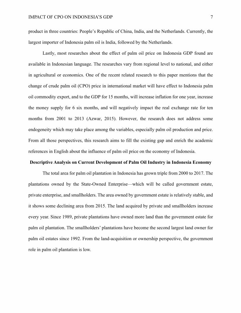
production output is used for export purpose. CPO dominates the palm oil industry products by

more than 80% from 2000 to 2017.

Figure 4. Composition of palm oil production from 2000 to 2017. Source: Indonesia

Statistics Office data.

CPO export volume shows increasing trend over year, and Palm oil kernel one is relatively

stable. For the year data ratio of export to production, it shows decreasing trend for both products.

The CPO export to production ratio in some periods is more than one which indicates the

interpretation that in those years, export tonnages were larger than the production volumes. Some

explanations for the miss-match are by doing import, or the CPO volume has become larger due

to some chemical addition process in some CPO derivative products. Despite the increase of

production volume, the increase of domestic demand may be one of the reasons in the declining

trend.

Figure 5. Palm oil product export volume and its ratio to production from 2000 to 2017.

Source: Indonesia Statistics Office data.

0%20%40%60%80%

100%

2000 2001 2002 2003 2004 2005 2006 2007 2008 2009 2010 2011 2012 2013 2014 2015 2016 2017

CPO Production Palm Oil Kernel Production

.6

.8

1

1.2

1.4

Ratio

5 million

10 million

15 million

20 million

25 million

30 million

Volum

e (ton

)

2000 2002 2004 2006 2008 2010 2012 2014 2016 2018

CPO Export Volume CPO Export to Production Ratio

.2

.3

.4

.5

.6

Ratio

500000

1 million

1.5 million

2 million

Vol

ume (

ton)

2000 2002 2004 2006 2008 2010 2012 2014 2016 2018

Palm Oil Kernel Volume Palm Oil Kernel Export to Production Ratio


CPO is the main export commodities in Indonesia. Other commodities after CPO are coal,

and oil. The proportion of CPO to total export has exceeded 10% since 2007, and the peak was in

2012 at 13.06%. The contribution average from 2000 to 2017 is 9%. Currently, Indonesia is the

largest producer and exporter country. Other major commodity, like coal, was the prime

commodities from 2009 until 2013, and Indonesia was proud as the second largest exporter country

(after Australia). Recently the fall of the coal commodity may still give bad impact on the economy.

Figure 6. The contribution of CPO export value to total export. Source: Indonesia

Statistics Office data, some is retrieved from Bank Indonesia website.

Indonesia economy shows the increasing trend of GDP in constant price (year 2000) from

2000 to 2018. For the GDP, the value has increased become more than double from 2000 to 2018.

Nevertheless, the annual growth rate of the GDP from its previous period varies from year to year,

as shown in the figure below. The growth rate is always positive, but it may be higher from the

previous period, or lower from the previous one. The positive growth rate implicates that GDP

value always increases for each period, but the amount increased may vary depending on the

growth rate itself. For the case in 2018, the fluctuation in the growth rate is suspected from the

fluctuation in the international price of palm oil, especially for quarterly GDP growth rate. Based

on that information, this paper will try to capture some interaction between the international palm

oil price and Indonesia GDP from 2000 to 2018.

0.002.004.006.008.00

10.0012.0014.00

2000

2001

2002

2003

2004

2005

2006

2007

2008

2009

2010

2011

2012

2013

2014

2015

2016

2017


Figure 7. Indonesia GDP and annual GDP growth from 2000 to 2018. Source: FED St.

Louis website.

After knowing the GDP—especially in the constant price—always increases over years,

the next necessary step is to conduct contribution/proportional analysis of palm oil sector,

especially CPO. Palm oil contributes to the GDP (the next data used is current price perspective)

from export side (based on expenditure approach), and from the plantation crops subsector (based

on production sector). One of the other reasons using current price data is because the price effect

has not yet omitted in the observed variables, like CPO export value. In 2018, the Government

targeted in the budget assumption that the economy (GDP) would grow at 5.4% year on year from

2017, but the realization was only 5.17%. In the quarterly period, the slow GDP growth in Q1 at

5.06% (below the expected 5.1%) was contributed by many factors, and one of them was the

decline in the CPO price.

The GDP classification by BPS as previously mentioned for agriculture, forestry, and

fishery sector can be further classified into agriculture, livestock, hunting, and agricultural

services; forestry and logging; and fishery. The plantation is positioned under the agriculture,

3

4

5

6

7

Annu

al GD

P grow

th rat

e in p

ercen

t

1000

1500

2000

2500

3000

GDP 2

000 i

n tril

lion I

ndon

esian

rupia

h

2000 2002 2004 2006 2008 2010 2012 2014 2016 2018

GDP GDP Growth rate


livestock, hunting, and agricultural services. The nominal value of the contribution can be seen in

the following graph.

Figure 8. The contribution of export and plantation sector in GDP (current price). Source:

Indonesia Statistics Office data, retrieved from Bank Indonesia website.

Nominally, the plantation sector and export relatively stable, which in the proportion

perspective, their contribution become smaller. For example, export to the GDP on average is

24.77% with the maximum point of 37% in 2000. From this perspective, the contribution palm oil

over the years should be illustrated in the proportion, as in the following graph. Also, the figure

includes new variables, which is CPO export value proportion.

Figure 9. The ratio proportion of plantation sector, export, and CPO export to GDP over

years. Source: Indonesia Statistics Office data, some are retrieved from Bank Indonesia website.

0

5 million

10 million

15 million

2000 2002 2004 2006 2008 2010 2012 2014 2016 2018

GDP in current price Plantation contribution value to GDPExport value

0%

10%

20%

30%

40%

2000 2002 2004 2006 2008 2010 2012 2014 2016 2018

Ratio of export to GDP Plantation proportion to GDPCPO export to GDP ratio


Although the trend shows that CPO export ratio is around 1 to 2% to GDP as the whole,

The highest proportion shown during the observation period is in 2011 (3.14%) and the lowest one

is in 2001 (0.89%), with the average of 2.12%. One of the interesting findings about the graph

about is the ratio of CPO export value to GDP exceed the trend of plantation sector contribution

to GDP from 2004 to 2014. The CPO export value in 2008, 2011, and 2012 exceeded the plantation

sector contribution. During that period, most of the CPO produced is mostly traded as export

commodities. The trend has reversed since 2014, probably it is because domestic demand for

industry supply-chain material increases. Also, in 2014, the Government once imposed export

levies USD50 for each ton volume to the CPO export. On average, the percentage of plantation

sector contribution to GDP is higher than the CPO export, and the value is 2.39%.

From the correlation test perspective, GDP in current price, export, and all the observed

variables during the period 2000 to 2018 are positively correlated. The coefficients for each two

variables tested can be found in the table below.

Table 1.

Coefficient of correlation of Indonesia GDP in current price, export value, plantation sector

contribution, and CPO export value during 2000 to 2018

No. Correlation Coefficient 1. GDP-export value 0.9602 2. GDP-plantation sector 0.9500 3. GDP-CPO export value 0.9021 4. Plantation sector-CPO export value 0.7232

Note: Source: FED St. Louis website, and Indonesia Statistics Office data, some are

retrieved from Bank Indonesia website

From the descriptive analysis perspective, the contribution of CPO export in Indonesia

economy, specifically GDP seems small, only 1-2% of the GDP, and it has positive coefficient of

correlation with the GDP.


Interaction between International Palm Oil Price and Indonesia GDP

This is the start of inferencing analysis part. The first step is conducting bivariate simple

regression by only using two variables. This regression aims at studying the relationship of

variables, in terms of how the dependent variable with changes in the independent variable. This

research only emphasizes on the impact (inferential purpose) rather than the other use of regression

for prediction. The assumption in this analysis is that the relationship between the two variables

are in the linear function. The common equation for this analysis is:

𝑦" = 𝛽% + 𝛽'𝑥" + 𝜀"

In that equation, 𝑦" is the dependent variable, and 𝑥" is the independent one. While, 𝛽%and

𝛽' are the parameter of the regression and 𝜀" is the random error term. The data used for this

regression part will be monthly data.

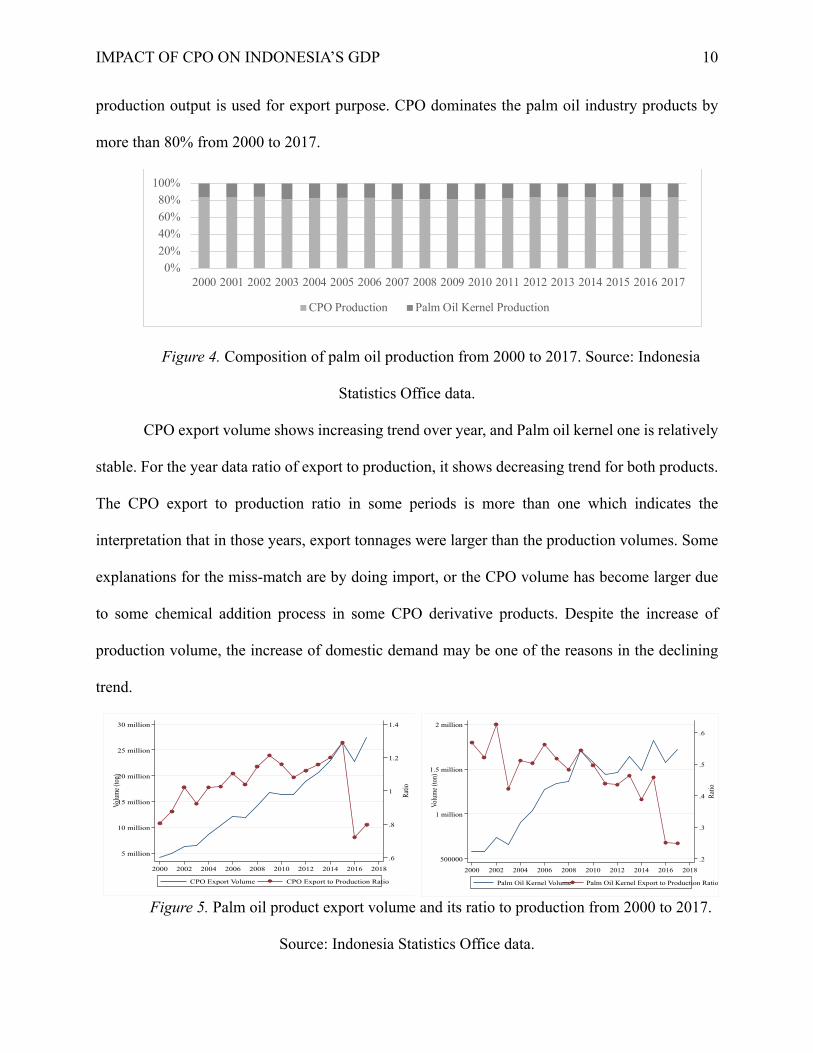
Figure 10. Composition of Indonesia CPO Export from 2000 to 2017. Source: Indonesia

Statistics Office data.

In international trade, Indonesia CPO is classified into two commodities based on the

Harmonized Standard (HS) System, which are CPO (HS 151110000) and Other CPO (HS

151119000). In the previous years, the portion of CPO (HS 151110000) commodity in the CPO

export was nearly 50% of the trade volume. Recently, the proportion has declined, but the average

is still high by 41.44% from 2000 to 2017. In my opinion, the CPO (HS 151110000) commodity

0%20%40%60%80%

100%

2000 2001 2002 2003 2004 2005 2006 2007 2008 2009 2010 2011 2012 2013 2014 2015 2016 2017

CPO Export Other CPO Export


can represent the CPO. For the regression analysis ahead, all CPO export data which will be used

is the HS 151110000 only. One of the considerations is because they have different HS, tariff rates

may be charged differently, and this research want to ignore the tariff which may influence export.

Here is the result of bivariate regression relationship between some palm oil and CPO data

variables that will be used further. The international price (of palm oil) defined in this research is

the data from Malaysia Palm Oil Futures (first contract forward) which is retrieved from the IMF

database. The variables of change of the previous variables are obtained by applying natural

logarithm function to the existing original data, which is commonly called as level data.

Table 2

Palm oil data bivariate regression result properties

No. Dependent variable

Independent variable

Regression Coefficient

Robust standard error

Probability not to reject null hypothesis

Goodness of fit

1. Export volume

Production -.0091041 .0408899 0.824 0.0003

2. Change in export volume

Change in production

.0897955 .1356018 0.509 0.0030

3. Export volume

International price

227.9559 98.98409 0.023 0.0379

4. Change in international price

Change in export volume

.2342176 .1279929 0.07 0.0266

Note: Source: Indonesia Statistics Office data and the IMF database.

Change in USD1 in the international palm oil price will increase the export volume become

228 ton, and the 1% change of the export volume will have impact on 0.23% change of the

international price. However, there is one uncommon finding in this bivariate regression, the

relationship between CPO export volume and palm oil total production is negative, and not

statistically significant, in both ways. In this paper, the level of confidence used is 95% to declare


whether it is statistically significant or not. Ideally, export should be some proportion of the

production volume, but this is not proven by the regression properties. The relationship of CPO

export volume and international price of palm oil is statistically significant, but in both ways,

which means some endogeneity issue may happen.

Further analysis is necessary if the price of palm oil is affected by the supply of Indonesian

palm oil. The relationship between the international price of palm oil and production volume will

be checked using temperature as the instrumental variable. Temperature is chosen rather than other

weather indicator like rainfall intensity, because nationally the average temperature in Indonesia

is same. The rainfall condition varies among regions and islands in Indonesia, the national average

may not reflect the regional one where there are many palm oil plantations. The temperature data

is retrieved from the World Bank database. The instrumental variable purposes to isolate part of

production supply that does not influence the international price of palm oil. The equation for this

analysis is:

𝑦" = 𝛽% + 𝛽'𝑥" + 𝜀"

𝑥" = 𝜋% + 𝜋'𝑍" + 𝜈"

The test will assume that from the supply side, the supply of palm oil (production volume) in

Indonesia as the largest producer and exporter country whether has effect or not to the price.

Dependent variable is international price of palm oil. At the same time, the production of palm oil

is influenced by the temperature. For the instrumental variable to be considered as valid, it is

supposed to fulfill the conditions that the instrument is relevant which is given when the correlation

between instrumental variable and independent variable is not zero (𝐶𝑜𝑟𝑟(𝑍"𝑋") ≠ 0), then the

instrument exogeneity condition when the correlation between instrumental variable and the model

error term should be zero (𝐶𝑜𝑟𝑟(𝑍"𝜀") = 0.


Table 3

Instrumental variable (temperature) regression result properties at the regression of

international price of palm oil on palm oil production

No. Indicator/Test Variable: Level data Variable: change (logarithm) data

Bivariate Multivariate Bivariate Multivariate 1. Durbin (score) 5.6404 .000714 4.50357 .180661 2. Probability not to reject null

hypothesis of Durbin endogeneity test

0.0176 0.9787 0.0338 0.6708

3. Wu-Hausman test 5.75826 .000693 4.55668 .175427 4. Probability not to reject null

hypothesis of Wu-Hausman endogeneity test

0.0178 0.9790 0.0347 0.6760

5. First stage F-test 27.1863 27.7897 25.0464 27.9101 6. Probability not to reject null

hypothesis of weakness of instrumental variable

0.000 0.000 0.000 0.000

Note: Source: reproduced from Indonesia Statistics Office data and the IMF database.

From the properties above, the use of temperature as instrumental variable is strong, either

when the variable is at level, or at logarithm. It means that either temperature is statistically

significant influencing the palm oil production, or the change in the temperature is statistically

significant to influence the change of palm oil production. The condition of instrument relevant

condition is fulfilled for both situations. However, the indicator of Wu-Hausman and Durbin show

that endogeneity issue still remains, which means that instrument exogeneity condition cannot be

fulfilled. Both the level and logarithm (change) variables regressions have the same situation.

Based on the result, the presence of endogeneity is still bias. The instrumental variable, either

temperature may have some correlation with the model error term, or the change of temperature

may have some correlation with its model error term. Further interpretation is that the temperature

and its change may have some relationship with other factors other than the palm oil production

and the change of palm oil production, that contribute to the international price of palm oil and the


change of international price. The model only satisfies the relevant condition. In order to conduct

appropriate analysis about the influence of international palm oil price on Indonesia GDP, the test

that can deal with some endogeneity issues should be chosen.

As additional analysis shown above, other perspective is replicating the model by using

additional independent variables (it becomes multivariate regression) to solve the endogeneity,

without making problem in the relevancy condition. For example, if adding the international price

of soybean, the result of the model test will be as in the above table. Soybean is used because it is

the second largest used vegetable oils after the palm oil. The two goods can be assumed as

substitution goods which react to the price change. Also, multicollinearity issue from adding

additional variable (through regressing it with the error term of the bivariate or by conducting

correlation test) does not take place. Nevertheless, the result is not same for the logarithm

regression analysis. By adding another independent variable which the change of international

soybean price into the analysis, the bias result of endogeneity still occurs. The endogeneity issue

cannot be resolved by the simply adding independent variables.

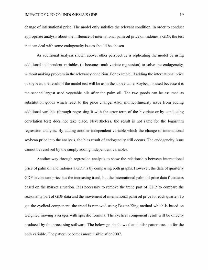
Another way through regression analysis to show the relationship between international

price of palm oil and Indonesia GDP is by comparing both graphs. However, the data of quarterly

GDP in constant price has the increasing trend, but the international palm oil price data fluctuates

based on the market situation. It is necessary to remove the trend part of GDP, to compare the

seasonality part of GDP data and the movement of international palm oil price for each quarter. To

get the cyclical component, the trend is removed using Baxter-King method which is based on

weighted moving averages with specific formula. The cyclical component result will be directly

produced by the processing software. The below graph shows that similar pattern occurs for the

both variable. The pattern becomes more visible after 2007.


Figure 11. Comparison of the pattern of palm oil price movement and GDP before at

level and logarithm data (above) and after (below) removing the trend component. Source: FED

St. Louis website and the IMF database.

By using bivariate regression where GDP cyclical component as the dependent variable,

the influence of price and the change of price are statistically significant on GDP, as shown in the

following table. Nevertheless, the influence of price and the change of price are not statistically

significant on the change in GDP cyclical component. If the international palm oil price change

USD1, the GDP will change by the local currency Indonesia rupiah IDR12 billion, and when the

price changes, increase by 1%, the GDP will also increase by IDR8.2 trillion. The parameters are

200

400

600

800

1000

1200

Inte

rnat

iona

l pal

m o

il pr

ice

(in

USD

)

1000

1500

2000

2500

3000G

DP

cont

ant p

rice

yea

r 20

00 (

in tr

illio

n In

done

sian

rup

iah)

2000q1 2005q1 2010q1 2015q1 2020q1

GDP International price

5

5.5

6

6.5

7

Loga

rithm

of i

nter

natio

nal p

alm

oil

pric

e

34.5

35

35.5

Loga

rithm

of G

DP

2000q1 2005q1 2010q1 2015q1 2020q1

Change of GDP Change of international palm oil price

200

400

600

800

1000

1200

Palm

oil p

rice (

in US

D)

0

-20

-15

-10

-5

5

GDP2

000 c

yclic

al co

mpon

ent f

rom bk

filte

r (in

Indon

esian

Rup

iah tr

illion

)

2000q1 2005q1 2010q1 2015q1 2020q1qdate

GDP2000 cyclical component Palm oil price


in the positive value, means the change will be in the same direction: if the price declines, it will

make the GDP decrease, from the period of 2000 to 2017.

Table 4

Bivariate regression combination of cyclical component of GDP on international palm oil price

No. Indicator/Test GDP on Price

Change of GDP on Price

GDP on Change of Price

Elasticity

1. Regression Coefficient 1.27e+10 -.002531 8.20e+12 -2.340616 2. Robust standard error 2.52e+09 .0037552 1.60e+12 3.338931 3. Probability not to reject

null hypothesis 0.000 0.516 0.000 0.499

4. Goodness of fit 0.2609 0.0643 0.2507 0.0673 Note: Source: FED St. Louis website and the IMF database.

Because endogeneity can make bias in the regression analysis, it will be better to choose

analysis which it will not become issue, like VAR. By this test, the nature of variable which

previously are dependent and independent changes become all endogenous. In the VAR method,

the general equation will be as follows:

𝑦6 = 𝑏% + 𝐵'𝑦69' + 𝐵:𝑦69' + ⋯+ 𝐵<𝑦<9' + 𝜀6

All the variables are in the form of 𝑛 × 1 vector, 𝑦6 = (𝑦'6, 𝑦:6, … , 𝑦B6)′. Which in the form of

matrix, the equation will be (for n variable and t time) as follow.

𝑏% = D𝛽'%𝛽:%⋮

𝛽B%F , 𝐵' = D

𝛽''(')𝛽':

(') ⋯ 𝛽'B(')

⋮ ⋱ ⋮𝛽B'(')𝛽B'

(') ⋯ 𝛽BB(')F , … , 𝐵< = D

𝛽''(<)𝛽':

(<) ⋯ 𝛽'B(<)

⋮ ⋱ ⋮𝛽B'(<)𝛽B'

(<) ⋯ 𝛽BB(<)F , 𝜀% = D

𝜀'6𝜀:6⋮

𝜀B6F

In this part, it will be compared the result by using the bivariate VAR and multivariate one

by adding palm oil export volume and palm oil production. Those two variables are considered

having the endogeneity issues that has occurred in the previous tests, also export is part of GDP

from the expenditure approach. The export data which will be used is the volume, because if using

the value, some adjustment for inflation (either price level or exchange rate) is necessary to be

conducted. The endogenous variable in the left-hand side is GDP, and endogenous variable in the


right-hand side is international price of palm oil, production, and export. The analysis will be

conducted either for the variable in the level data and for the both changes (logarithm) data for the

change of GDP and change of international palm oil price.

Before conducting the VAR test, it is to check the stationarity condition of all the observed

variables. VAR result may be bias when one of the variables has unit roots. If the variables are not

stationer at the level data (original), they must be differenced to make it become stationer. One of

the popular methods to test stationarity is using Dickey-Fuller. The software result of this test for

the observed variables, and the first differencing level is shown in the below table. At level data,

either for level data or for logarithm data, the only stationer variable is palm oil export, which

means it does not need further differencing process.

Table 5

Result of stationarity test of the variables

No. Variable Level data Logarithm data Test-statistics Z(t)

MacKinnon approximate p-value for Z(t)

Test-statistics Z(t)

MacKinnon approximate p-value for Z(t)

1. GDP 8.857 1.0000 0.662 0.9890 2. First difference in GDP -5.629 0.0000 -10.825 0.0000 3. Palm oil price -1.794 0.3836 -1.736 0.4128 4. First difference in palm oil price -5.901 0.0000 -6.279 0.0000 5. Palm oil production -2.061 0.2604 -2.381 -2.381 6. First difference in palm oil

production -8.375 0.0000 -8.243 0.0000

7. Palm oil export -4.840 0.0000 -4.787 0.0001 Note: Source: FED St. Louis website, the IMF database, and Indonesia Statistics Office data.

When all the variables satisfy the stationer condition, the second step in VAR is choosing

the lag. Common methods which are suggested, especially by software, are likelihood ratio, final

prediction error (FPE), Akaike’s information criterion (AIC), Schwarz’s Bayesian information

criterion (SBIC), and the Hannan and Quinn information criterion (HQIC). The result of the tests,


for both bivariate and multivariate one, is shown in the table below. From the recommendation for

the level data (GDP, international palm oil price, palm oil production, and export volume), the lag

for bivariate is 2 and for multivariate is 4. For the multivariate, the lag is selected based on

comparing the result of all tests, and most tests advise 4. Meanwhile, for the logarithm data (change

of GDP, change of international price of palm oil, change of palm oil production, and change of

palm oil export), the lag recommendation is 4, and it is same with the lag recommendation result

at the level data. The analysis of data in this part is conducted from quarterly data, for example, if

the lag recommendation is 4, it can be interpreted as 4 quarters or 1 year in the future.

Table 6

Result of lag recommendation

No. Test Level data Logarithm data Bivariate Multivariate Bivariate Multivariate 1. Likelihood ratio 2 4 3 4 2. FPE suggestion 2 4 3 4 3. AIC suggestion 2 4 3 4 4. SBIC suggestion 2 1 2 0 5. HQIC suggestion 2 2 0 0

Note: Source: FED St. Louis website, the IMF database, and Indonesia Statistics Office data.

The third step is by conducting the VAR test itself. All endogenous variables are tested

based on their recommended lag, 2 for bivariate at level data 3 for bivariate at logarithm data, and

4 for multivariate. The result from bivariate VAR at level data declares that effect difference in

GDP is statistically significant for itself. The result for bivariate VAR at logarithm data displays

that the effect is not statistically significant neither for change of GDP on the change of GDP 3

quarters ahead, nor the change of price on the change of GDP. Meanwhile, for the multivariate

VAR, the result of difference in GDP and difference in palm oil price are statistically significant

on the difference in GDP in the 4 quarters in the future for the level data, but not for the logarithm

data.


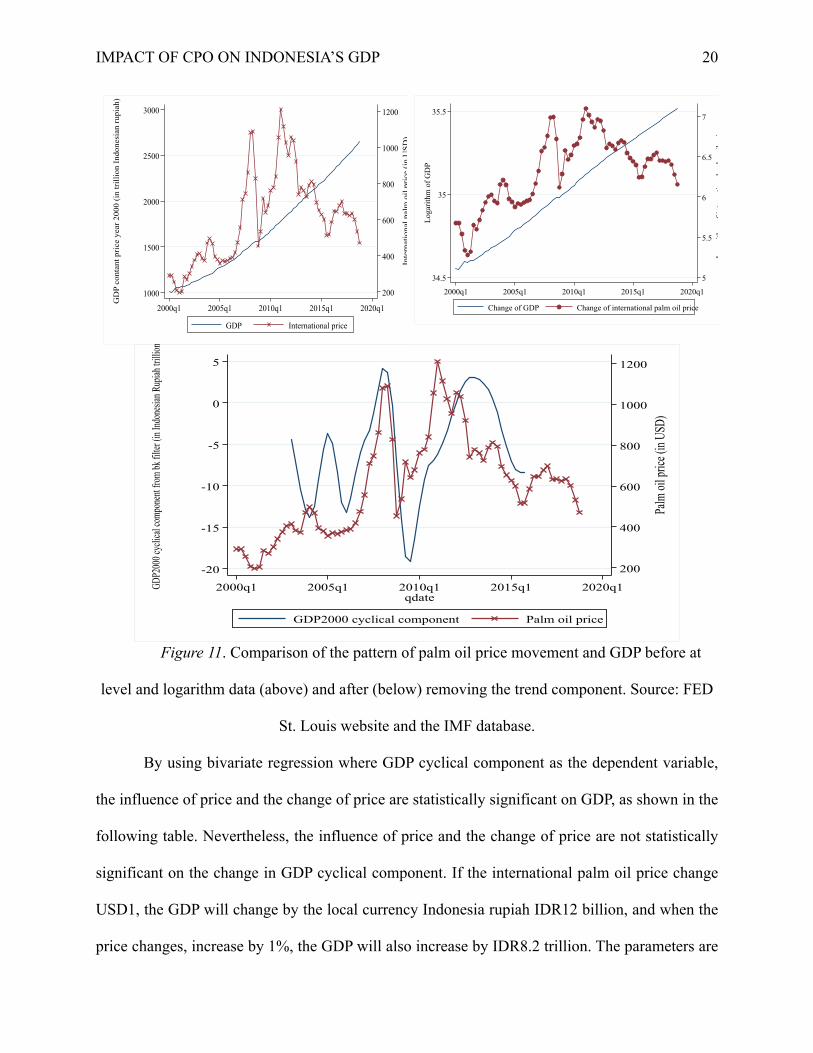
Table 7

Probability result that endogenous variables influence other variables

No. Variable Level data Logarithm data Bivariate Multivariate Bivariate Multivariate

1. GDP on GDP 0.000* 0.000* 0.716 0.012* 2. GDP on palm oil price 0.555 0.017* 0.411 0.181 3. GDP on palm oil production - 0.422 - 0.623 4. GDP on palm oil export - 0.958 - 0.718 5. Palm oil price on GDP 0.150 0.731 0.206 0.046* 6. Palm oil price on palm oil price 0.035* 0.739 0.358 0.424 7. Palm oil price on production - 0.283 - 0.191 8. Palm oil price on export - 0.755 - 0.678 9. Production on GDP - 0.225 - 0.154 10. Production on palm oil price - 0.717 - 0.570 11. Production on production - 0.008* - 0.011* 12. Production of export - 0.325 - 0.676 13. Export on GDP - 0.018* - 0.503 14. Export on palm oil price - 0.658 - 0.697 15. Export on production - 0.835 - 0.782 16. Export on export - 0.028* - 0.099

Note: *statistically significant result. Source: FED St. Louis website, the IMF database, and


The interpretation of the statistically significant result of the VAR analysis above is that for

the bivariate VAR for level data, the GDP of the current period will influence the GDP in the 2

quarters in the future, and the palm oil price in current period will influence itself in the 2 quarters

in the future. For the multivariate VAR in the level data, the GDP and palm oil price in the current

period will influence the GDP in the 4 quarters (1 year) in the future, also the palm oil production

in the current period will influence the production in the next 4 quarters, the GDP and palm oil

export in the current period will influence the palm oil export in the next 4 quarters. There is not

any significant result for bivariate VAR for the logarithm level data. For the multivariate VAR of

the logarithm data, the change in the GDP in the current period will influence the change of GDP

and the change of palm oil international price in the 4 quarters in the future, also the change of


production in the current period will influence the change of production in the 4 quarters in the

future.

Further posttest is necessary to assess the recommendation from VAR result, and one of

those is through Granger causality. For the bivariate model, Granger casualty result is not

statistically significant in both level and logarithm variables. The statically significant result for

the multivariate model occurs for both level and logarithm variables. For the level one, Granger

causality relationships are statistically significant between the difference in international palm oil

price and difference in GDP, also between CPO export volume and difference in GDP. In the

logarithm one, it is statistically significant that between the change in the GDP and the change of

international palm oil price. Granger casualty implies the two-way interaction between the

variables which influence each other, for the certain lag observed. The probability result from the

VAR table and Granger causality table for the statistically significant result are same. The result in

the Granger causality eliminates the causality which occurs through one variable the unilaterally

among different period.

Table 8

Probability result of Granger causality that implies statistically significant result

No. Variable Multivariate VAR Level Logarithm

1. GDP on palm oil price 0.017 - 2. Export volume on GDP 0.018 - 3. Palm oil price on GDP - 0.046

Note: Source: FED St. Louis website, the IMF database, and Indonesia Statistics Office.

The final step in VAR analysis to understand the impact is by conducting the impulse

response function. The table result of IRF analysis displays the same probability result as in the

VAR table previously. This result, graph, will illustrate the effect on certain variable when shock

(respective variable change) is given. Below is the result for the bivariate models.


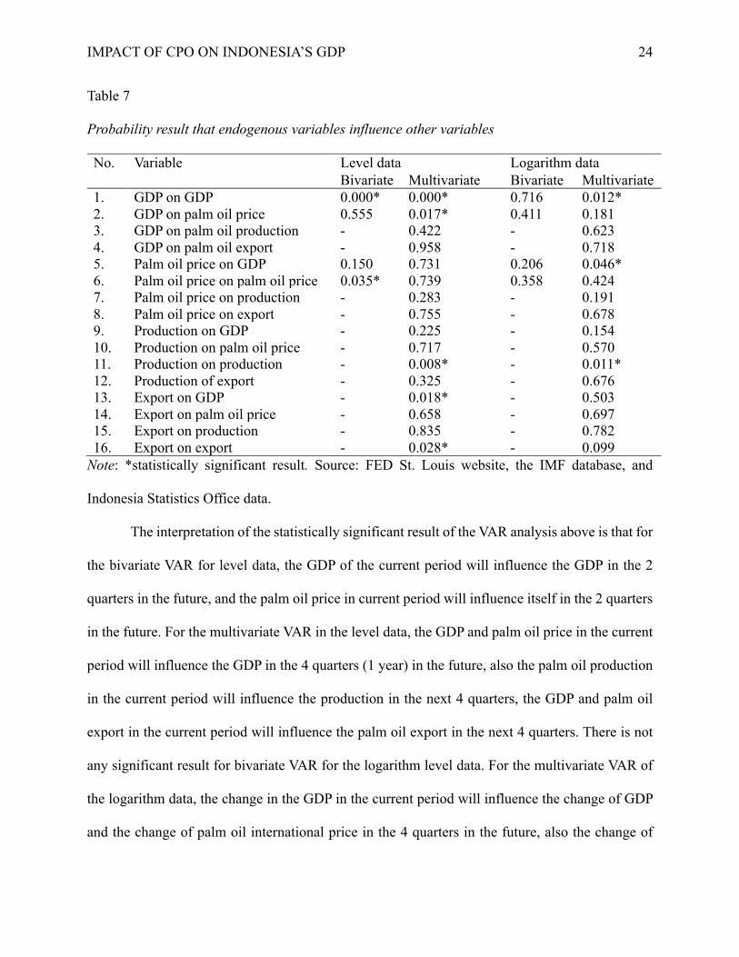
Figure 12. IRF graph from bivariate VAR at level data (left) and logarithm (right).

Source: reproduced from FED St. Louis website, the IMF database, and Indonesia Statistics

Office.

For the bivariate VAR, in the level data, the IRF result of palm oil price effect to GDP is

not available, but here is the interpretation of all shown graph. When the GDP changes, it will

affect itself continuously, and the value is always greater than 0. The effect will die out at period

7, or the seventh quarter. The GDP change effect stabilizes every 2 quarters, and it is statistically

significant. Also, at the level data, when the GDP declines in the first period, it will give effect to

the palm oil price, but it may be increase in price or decrease in price, then it becomes zero in the

third period. The effect occurs each two quarters, it will die out in the seventh quarter, but it is not

statistically significant. At the logarithm data, the percent change of palm oil price to the percent

change GDP will decline in the first period, increase again in the third period, and becomes zero

in the fifth quarter. The effect repeatedly occurs each two quarters and will die out in the seventh

quarter. Also, the percent change of palm oil price will affect itself, and the effect will die out after

the seventh quarter. Both effects in the logarithm data are not statistically significant, which by the

figure, the effect may be positive or negative (1% change of the palm oil price may make GDP

change from -0.01% to 0.05% in the first quarter, 0 in second quarter).

-5.000e+12

0

5.000e+12

1.000e+13

-5.000e+12

0

5.000e+12

1.000e+13

0 2 4 6 8 0 2 4 6 8

varbasic, d1gdp, d1gdp varbasic, d1gdp, d1palmoilprice

varbasic, d1palmoilprice, d1gdp varbasic, d1palmoilprice, d1palmoilprice

95% CI orthogonalized irf

step

Graphs by irfname, impulse variable, and response variable

-.05

0

.05

.1

.15

-.05

0

.05

.1

.15

0 2 4 6 8 0 2 4 6 8

varbasic, d1lgdp, d1lgdp varbasic, d1lgdp, d1lprice

varbasic, d1lprice, d1lgdp varbasic, d1lprice, d1lprice


step



Considering that the IRF graph result which is statistically significant is only one, the effect

of GDP to itself, it may not answer the question from this research. However, the IRF graph result

from the effect percent change of palm oil price to percent change of GDP may relate to the

research question, but it is difficult to exactly conclude whether the its increase will increase or

decrease the percent change of GDP, vice versa.

Figure 13. IRF graph from multivariate VAR at level data. Source: FED St. Louis

website, the IMF database, and Indonesia Statistics Office data.

-2.000e+12

0

2.000e+12

4.000e+12

6.000e+12

-2.000e+12

0

2.000e+12

4.000e+12

6.000e+12

-2.000e+12

0

2.000e+12

4.000e+12

6.000e+12

-2.000e+12

0

2.000e+12

4.000e+12

6.000e+12

0 2 4 6 8 0 2 4 6 8 0 2 4 6 8 0 2 4 6 8

varbasic, CPOExportVolume, CPOExportVolume varbasic, CPOExportVolume, d1gdp varbasic, CPOExportVolume, d1palmoilprice varbasic, CPOExportVolume, d1prod

varbasic, d1gdp, CPOExportVolume varbasic, d1gdp, d1gdp varbasic, d1gdp, d1palmoilprice varbasic, d1gdp, d1prod

varbasic, d1palmoilprice, CPOExportVolume varbasic, d1palmoilprice, d1gdp varbasic, d1palmoilprice, d1palmoilprice varbasic, d1palmoilprice, d1prod

varbasic, d1prod, CPOExportVolume varbasic, d1prod, d1gdp varbasic, d1prod, d1palmoilprice varbasic, d1prod, d1prod


step


-.2

0

.2

.4

-.2

0

.2

.4

-.2

0

.2

.4

-.2

0

.2

.4

0 2 4 6 8 0 2 4 6 8 0 2 4 6 8 0 2 4 6 8

varbasic, d1lgdp, d1lgdp varbasic, d1lgdp, d1lprice varbasic, d1lgdp, d1lprod varbasic, d1lgdp, lexport

varbasic, d1lprice, d1lgdp varbasic, d1lprice, d1lprice varbasic, d1lprice, d1lprod varbasic, d1lprice, lexport

varbasic, d1lprod, d1lgdp varbasic, d1lprod, d1lprice varbasic, d1lprod, d1lprod varbasic, d1lprod, lexport

varbasic, lexport, d1lgdp varbasic, lexport, d1lprice varbasic, lexport, d1lprod varbasic, lexport, lexport


step



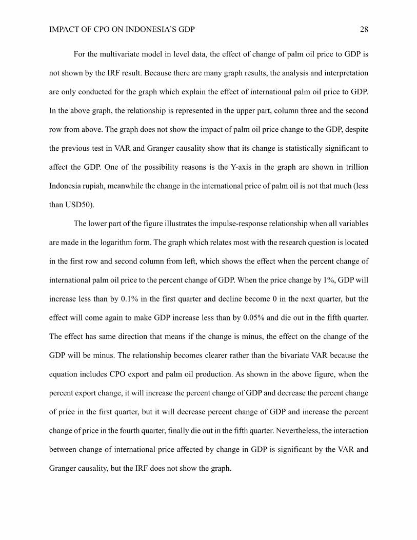
For the multivariate model in level data, the effect of change of palm oil price to GDP is

not shown by the IRF result. Because there are many graph results, the analysis and interpretation

are only conducted for the graph which explain the effect of international palm oil price to GDP.

In the above graph, the relationship is represented in the upper part, column three and the second

row from above. The graph does not show the impact of palm oil price change to the GDP, despite

the previous test in VAR and Granger causality show that its change is statistically significant to

affect the GDP. One of the possibility reasons is the Y-axis in the graph are shown in trillion

Indonesia rupiah, meanwhile the change in the international price of palm oil is not that much (less

than USD50).

The lower part of the figure illustrates the impulse-response relationship when all variables

are made in the logarithm form. The graph which relates most with the research question is located

in the first row and second column from left, which shows the effect when the percent change of

international palm oil price to the percent change of GDP. When the price change by 1%, GDP will

increase less than by 0.1% in the first quarter and decline become 0 in the next quarter, but the

effect will come again to make GDP increase less than by 0.05% and die out in the fifth quarter.

The effect has same direction that means if the change is minus, the effect on the change of the

GDP will be minus. The relationship becomes clearer rather than the bivariate VAR because the

equation includes CPO export and palm oil production. As shown in the above figure, when the

percent export change, it will increase the percent change of GDP and decrease the percent change

of price in the first quarter, but it will decrease percent change of GDP and increase the percent

change of price in the fourth quarter, finally die out in the fifth quarter. Nevertheless, the interaction

between change of international price affected by change in GDP is significant by the VAR and

Granger causality, but the IRF does not show the graph.


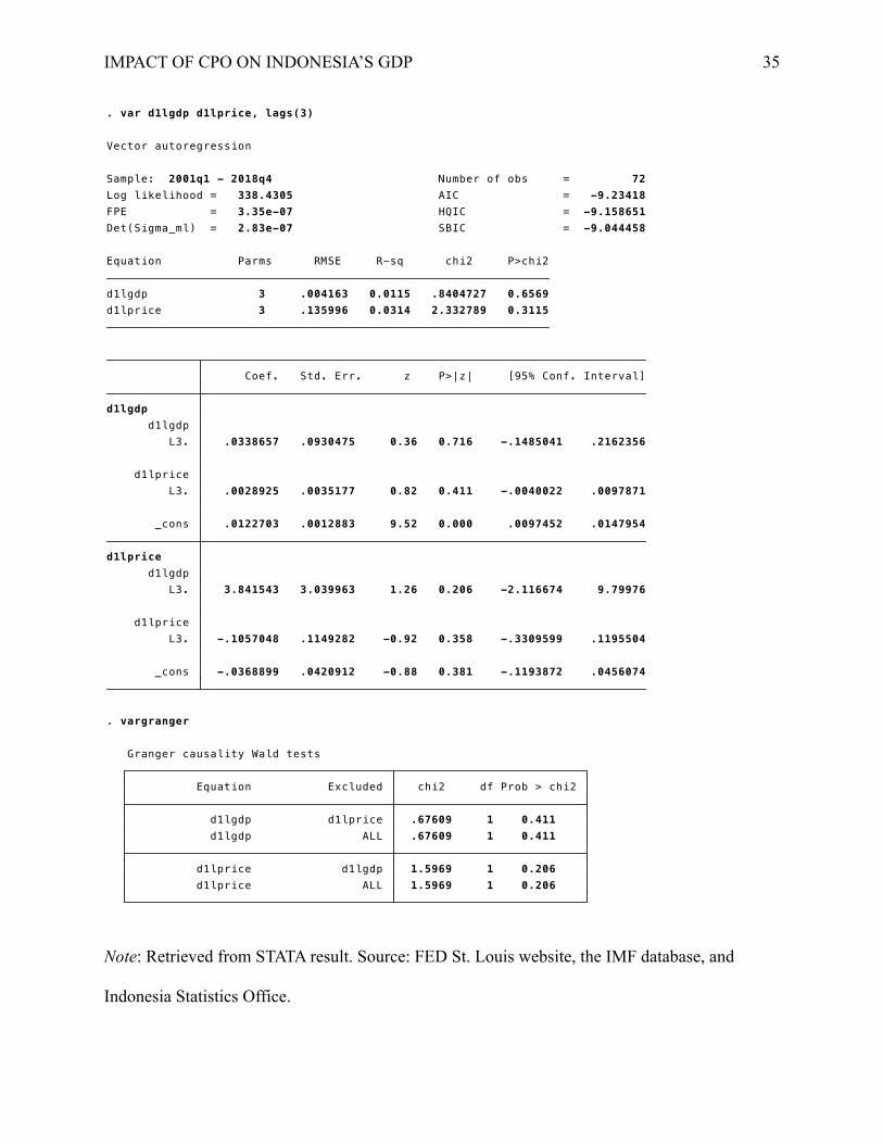
The consistent results among VAR test, Granger causality, IRF for two different variables

are only between international palm oil price with GDP and change of GDP with change of

international palm oil price. Nevertheless, the effect is not fully for 4 lags consecutively as

recommended by VAR test, but in the first quarter and from the third to the fifth one. Through IRF,

the effect will die out in the second quarter after 5 quarters.

Conclusion and Recommendation

Palm oil sector in Indonesia has grown positively from 2000 to 2017 which was shown by

many increasing indicators like total area for palm oil plantation in Indonesia has grown triple,

production has increased more than six times, and CPO export has increased triple, in average is

9% to total goods export. From the graph of land used for palm oil plantation if the growth is

constant, there will some tendency that in the future the smallholders’ total area for may exceed

the private plantation. The major product from palm oil is CPO by more than 80% and mainly

produced as export commodity, the average ratio between CPO export to ratio is 1.03 means most

of the production is for export, and 41.44% of that CPO consists of CPO purely. The correlation

between GDP and CPO export value is positive and displays high coefficient number (0.9).

From the regression analysis, endogeneity issues arise from the relationship of international

palm oil price with palm oil production in Indonesia. Export volume is also influenced significantly

by the international palm oil price, but not by the national production. There is an interesting

finding on the relationship between CPO export volume and palm oil production, that it is not

statistically significant. After goods and services being produced, some part of them supposed to

be traded to the rest of the world as export, but that case is not found within this research using

bivariate regression. After removing the trend, the regression analysis of GDP cyclical component


on international palm oil price shows significant result, which means that the price influences the

GDP. If price change positively by USD1, the GDP will increase by IDR12 billion, and when it

increases by 1%, the GDP will also increase by IDR8.2 trillion, vice versa when it declines.

By further analysis using VAR method, the effect of international palm oil price fluctuation

to Indonesia GDP is statistically significant while using the multivariate VAR. There is causality

relationship between palm oil price to GDP if the price change by 1%, GDP will increase by less

than 0.1% in the first quarter and decline become 0 in the second quarter, but the effect will come

again to make GDP increase less than by 0.05% and die out in the fifth quarter. From VAR and

Granger causality result, the change of international palm oil price is affected by the change in

Indonesia GDP, but the IRF does not provide the graph. Either bivariate or multivariate VAR

suggests that the change in the GDP will affect the GDP itself.

For stakeholders in the palm oil sector, they should aware about the effect which cause by

that commodity price fluctuation. For private sector, usually they are more flexible to mitigate the

risk by some hedging mechanism, like having future contracts. For government, it is better to

consider the timing whether the to include international price of palm oil (like other commodities

like oil) as surveillance indicator. Also, some data shows that the ratio of production to total area

(tonnage/hectare) for government estate is the most fluctuated one. It is important to make the ratio

become more stable, proportional between the production to total area, or the government may

further reduce its share and leave this sector to the private sector. From academic perspective,

further research and better modelling in CPO should be explored for the exact impact in the future.

Another aspect for research improvement is by the perspective of regionalism for some largest

provinces which CPO is their main commodity, probably their regional GDP will be affected more

than the Indonesian national GDP by the price change.


References

Amzul, Rifin. (2011). The Role of Palm Oil Industry in Indonesian Economy and Its Export

Competitiveness. Retrieved from: https://repository.dl.itc.u-

tokyo.ac.jp/?action=repository_action_common_download&item_id=4186&item_no=1&

attribute_id=14&file_no=1

Azwar. (2015). Dampak Perubahan Harga Crude Palm Oil (CPO) Dunia terhadap Value Ekspor

Komoditas Kelapa Sawit dan Perekonomian Indonesia (Pendekatan Vector

Autoregression Analysis). Jurnal Info Artha Sekolah Tinggi Akuntansi Negara (STAN)

Vol.I/XIII/2015. Retrieved from

https://www.academia.edu/27053014/DAMPAK_PERUBAHAN_HARGA_CRUDE_PA

LM_OIL_CPO_DUNIA_TERHADAP_VALUE_EKSPOR_KOMODITAS_KELAPA_S

AWIT_DAN_PEREKONOMIAN_INDONESIA_PENDEKATAN_VECTOR_AUTORE

GRESSION_ANALYSIS_?auto=download

Ghalayini, Latife. (2011). The Interaction between Oil Price and Economic Growth. Middle

Eastern Finance and Economics, SSN: 1450-2889 Issue 13 (2011), Pages From 127 To

141.

International Monetary Fund. (2017). Indonesia 2017 Article IV Consultation.

Kilian, Lutz, and Vigfusson, Robert J. (2016). The Role of Oil Price Shocks in Causing US

Recession. CESIFO Working Paper No. 5743 Category 10: Energy and Climate

Economics.


Additional Tables

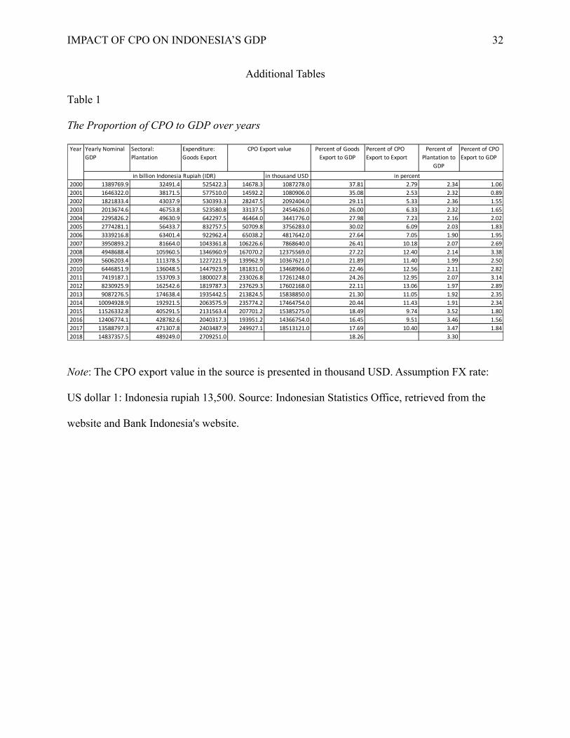
Table 1

The Proportion of CPO to GDP over years

Note: The CPO export value in the source is presented in thousand USD. Assumption FX rate:

US dollar 1: Indonesia rupiah 13,500. Source: Indonesian Statistics Office, retrieved from the

website and Bank Indonesia's website.

Yearly Nominal GDP

Sectoral: Plantation

Expenditure: Goods Export

Percent of Goods Export to GDP

Percent of CPO Export to Export

Percent of Plantation to

GDP

Percent of CPO Export to GDP

in thousand USD2000 1389769.9 32491.4 525422.3 14678.3 1087278.0 37.81 2.79 2.34 1.062001 1646322.0 38171.5 577510.0 14592.2 1080906.0 35.08 2.53 2.32 0.892002 1821833.4 43037.9 530393.3 28247.5 2092404.0 29.11 5.33 2.36 1.552003 2013674.6 46753.8 523580.8 33137.5 2454626.0 26.00 6.33 2.32 1.652004 2295826.2 49630.9 642297.5 46464.0 3441776.0 27.98 7.23 2.16 2.022005 2774281.1 56433.7 832757.5 50709.8 3756283.0 30.02 6.09 2.03 1.832006 3339216.8 63401.4 922962.4 65038.2 4817642.0 27.64 7.05 1.90 1.952007 3950893.2 81664.0 1043361.8 106226.6 7868640.0 26.41 10.18 2.07 2.692008 4948688.4 105960.5 1346960.9 167070.2 12375569.0 27.22 12.40 2.14 3.382009 5606203.4 111378.5 1227221.9 139962.9 10367621.0 21.89 11.40 1.99 2.502010 6446851.9 136048.5 1447923.9 181831.0 13468966.0 22.46 12.56 2.11 2.822011 7419187.1 153709.3 1800027.8 233026.8 17261248.0 24.26 12.95 2.07 3.142012 8230925.9 162542.6 1819787.3 237629.3 17602168.0 22.11 13.06 1.97 2.892013 9087276.5 174638.4 1935442.5 213824.5 15838850.0 21.30 11.05 1.92 2.352014 10094928.9 192921.5 2063575.9 235774.2 17464754.0 20.44 11.43 1.91 2.342015 11526332.8 405291.5 2131563.4 207701.2 15385275.0 18.49 9.74 3.52 1.802016 12406774.1 428782.6 2040317.3 193951.2 14366754.0 16.45 9.51 3.46 1.562017 13588797.3 471307.8 2403487.9 249927.1 18513121.0 17.69 10.40 3.47 1.842018 14837357.5 489249.0 2709251.0 18.26 3.30

in billion Indonesia Rupiah (IDR)

CPO Export valueYear

in percent


Table 2

Lag selection for VAR analysis

Note: Retrieved from STATA result. Source: FED St. Louis website, the IMF database, and

Indonesia Statistics Office.

Exogenous: _cons Endogenous: d1gdp d1palmoilprice d1prod CPOExportVolume 4 -2767.34 53.56* 16 0.000 2.6e+52* 131.876* 132.903 134.661 3 -2794.12 27.699 16 0.034 3.9e+52 132.378 133.163 134.508 2 -2807.97 58.339 16 0.000 3.4e+52 132.278 132.821* 133.752 1 -2837.14 40.096 16 0.001 6.1e+52 132.89 133.192 133.709 0 -2857.19 7.3e+52 133.078 133.139 133.242* lag LL LR df p FPE AIC HQIC SBIC Sample: 2007q2 - 2017q4 Number of obs = 43 Selection-order criteria

. varsoc d1gdp d1palmoilprice d1prod CPOExportVolume

Exogenous: _cons Endogenous: d1gdp d1palmoilprice 4 -2573.59 4.9865 4 0.289 1.7e+29 73.0026 73.2308 73.5763 3 -2576.09 3.4788 4 0.481 1.7e+29 72.9602 73.1376 73.4064 2 -2577.83 43.999* 4 0.000 1.6e+29* 72.8965* 73.0233* 73.2152* 1 -2599.83 53.867 4 0.000 2.6e+29 73.4035 73.4796 73.5948 0 -2626.76 4.9e+29 74.0496 74.0749 74.1133 lag LL LR df p FPE AIC HQIC SBIC Sample: 2001q2 - 2018q4 Number of obs = 71 Selection-order criteria

. varsoc d1gdp d1palmoilprice

Exogenous: _cons Endogenous: d1lgdp d1lprice d1lprod lexport 4 309.126 43.909* 16 0.000 1.9e-10* -11.2152* -10.1881 -8.43 3 287.171 33.76 16 0.006 2.3e-10 -10.9382 -10.1528 -8.80838 2 270.291 37.643 16 0.002 2.2e-10 -10.8973 -10.3535 -9.42278 1 251.47 40.862 16 0.001 2.5e-10 -10.766 -10.464 -9.94688 0 231.039 3.0e-10 -10.56 -10.4995* -10.3961* lag LL LR df p FPE AIC HQIC SBIC Sample: 2007q2 - 2017q4 Number of obs = 43 Selection-order criteria

. varsoc d1lgdp d1lprice d1lprod lexport

Exogenous: _cons Endogenous: d1lgdp d1lprice 4 364.51 1.8262 4 0.768 2.0e-07 -9.76086 -9.53274 -9.18722 3 363.597 11.077* 4 0.026 1.8e-07* -9.84781* -9.67039 -9.40165 2 358.059 17.667 4 0.001 1.9e-07 -9.80447 -9.67774* -9.48579 1 349.225 7.4372 4 0.115 2.2e-07 -9.66832 -9.59228 -9.47711 0 345.507 2.2e-07 -9.67625 -9.6509 -9.61251* lag LL LR df p FPE AIC HQIC SBIC Sample: 2001q2 - 2018q4 Number of obs = 71 Selection-order criteria

. varsoc d1lgdp d1lprice


Table 3

VAR and Granger result for bivariate analysis

d1palmoilprice ALL . 0 . d1palmoilprice d1gdp . 0 . d1gdp ALL .34895 1 0.555 d1gdp d1palmoilprice .34895 1 0.555 Equation Excluded chi2 df Prob > chi2 Granger causality Wald tests

. vargranger

_cons 40.319 27.15063 1.49 0.138 -12.89526 93.53325 L2. -.2379498 .1129566 -2.11 0.035 -.4593407 -.0165589d1palmoilprice L2. -1.68e-12 1.17e-12 -1.44 0.150 -3.97e-12 6.08e-13 d1gdp d1palmoilprice

_cons 1.16e+13 2.22e+12 5.24 0.000 7.29e+12 1.60e+13 L2. -5.46e+09 9.24e+09 -0.59 0.555 -2.36e+10 1.26e+10d1palmoilprice L2. .4918176 .0955467 5.15 0.000 .3045494 .6790857 d1gdp d1gdp

Coef. Std. Err. z P>|z| [95% Conf. Interval]

d1palmoilprice 3 88.0673 0.0891 4.437593 0.1087d1gdp 3 7.2e+12 0.2664 26.50782 0.0000

Equation Parms RMSE R-sq chi2 P>chi2

Det(Sigma_ml) = 3.57e+29 SBIC = 74.0765FPE = 4.21e+29 HQIC = 73.96327Log likelihood = -2690.921 AIC = 73.88825Sample: 2000q4 - 2018q4 Number of obs = 73

Vector autoregression

. var d1gdp d1palmoilprice, lags(2)




.

d1lprice ALL 1.5969 1 0.206 d1lprice d1lgdp 1.5969 1 0.206 d1lgdp ALL .67609 1 0.411 d1lgdp d1lprice .67609 1 0.411 Equation Excluded chi2 df Prob > chi2 Granger causality Wald tests

. vargranger

_cons -.0368899 .0420912 -0.88 0.381 -.1193872 .0456074 L3. -.1057048 .1149282 -0.92 0.358 -.3309599 .1195504 d1lprice L3. 3.841543 3.039963 1.26 0.206 -2.116674 9.79976 d1lgdp d1lprice

_cons .0122703 .0012883 9.52 0.000 .0097452 .0147954 L3. .0028925 .0035177 0.82 0.411 -.0040022 .0097871 d1lprice L3. .0338657 .0930475 0.36 0.716 -.1485041 .2162356 d1lgdp d1lgdp


d1lprice 3 .135996 0.0314 2.332789 0.3115d1lgdp 3 .004163 0.0115 .8404727 0.6569


Det(Sigma_ml) = 2.83e-07 SBIC = -9.044458FPE = 3.35e-07 HQIC = -9.158651Log likelihood = 338.4305 AIC = -9.23418Sample: 2001q1 - 2018q4 Number of obs = 72


. var d1lgdp d1lprice, lags(3)


Table 4

VAR and Granger result for multivariate analysis

_cons 2309109 493351.4 4.68 0.000 1342158 3276060 L4. .2827281 .1284865 2.20 0.028 .0308991 .534557CPOExportVolume L4. .0177913 .0855564 0.21 0.835 -.1498962 .1854789 d1prod L4. 314.5831 709.6736 0.44 0.658 -1076.352 1705.518 d1palmoilprice L4. -3.92e-08 1.65e-08 -2.37 0.018 -7.16e-08 -6.73e-09 d1gdp CPOExportVolume

_cons 1272531 814797.7 1.56 0.118 -324442.9 2869505 L4. -.2088845 .2122028 -0.98 0.325 -.6247943 .2070253CPOExportVolume L4. .3723397 .1413013 2.64 0.008 .0953943 .6492852 d1prod L4. 424.8039 1172.066 0.36 0.717 -1872.403 2722.011 d1palmoilprice L4. -3.32e-08 2.73e-08 -1.21 0.225 -8.68e-08 2.04e-08 d1gdp d1prod

_cons -49.55435 112.0077 -0.44 0.658 -269.0854 169.9767 L4. 9.12e-06 .0000292 0.31 0.755 -.0000481 .0000663CPOExportVolume L4. .0000208 .0000194 1.07 0.283 -.0000172 .0000589 d1prod L4. .0535914 .1611202 0.33 0.739 -.2621985 .3693813 d1palmoilprice L4. 1.29e-12 3.76e-12 0.34 0.731 -6.07e-12 8.65e-12 d1gdp d1palmoilprice

_cons 1.12e+13 4.22e+12 2.65 0.008 2.91e+12 1.95e+13 L4. -57550.7 1100013 -0.05 0.958 -2213537 2098436CPOExportVolume L4. 587915.2 732475.2 0.80 0.422 -847710 2023540 d1prod L4. -1.45e+10 6.08e+09 -2.39 0.017 -2.64e+10 -2.60e+09 d1palmoilprice L4. .5911261 .1416766 4.17 0.000 .3134451 .868807 d1gdp d1gdp


CPOExportVolume 5 517205 0.2229 12.33445 0.0150d1prod 5 854194 0.1948 10.40484 0.0341d1palmoilprice 5 117.423 0.0361 1.512762 0.8244d1gdp 5 4.4e+12 0.2997 18.40419 0.0010




. var d1gdp d1palmoilprice d1prod CPOExportVolume, lags(4)

_cons 11.27598 2.005053 5.62 0.000 7.346147 15.20581 L4. .2296142 .139094 1.65 0.099 -.0430051 .5022335 lexport L4. .0818565 .296241 0.28 0.782 -.4987652 .6624781 d1lprod L4. .1454677 .3735727 0.39 0.697 -.5867214 .8776568 d1lprice L4. -13.85493 20.68828 -0.67 0.503 -54.40321 26.69336 d1lgdp lexport

_cons .5870696 .9314072 0.63 0.528 -1.238455 2.412594 L4. -.0270418 .0646133 -0.42 0.676 -.1536816 .0995981 lexport L4. .3488808 .1376128 2.54 0.011 .0791647 .618597 d1lprod L4. .098548 .1735357 0.57 0.570 -.2415757 .4386718 d1lprice L4. -13.6847 9.610326 -1.42 0.154 -32.52059 5.151196 d1lgdp d1lprod

_cons -.6624898 .9567114 -0.69 0.489 -2.53761 1.21263 L4. .0275497 .0663687 0.42 0.678 -.1025307 .15763 lexport L4. .1848411 .1413514 1.31 0.191 -.0922026 .4618848 d1lprod L4. -.142369 .1782503 -0.80 0.424 -.4917331 .2069952 d1lprice L4. 19.68092 9.871417 1.99 0.046 .3332952 39.02854 d1lgdp d1lprice

_cons .013486 .0171112 0.79 0.431 -.0200514 .0470233 L4. -.0004286 .001187 -0.36 0.718 -.0027551 .0018979 lexport L4. .0012413 .0025281 0.49 0.623 -.0037138 .0061963 d1lprod L4. -.0042634 .0031881 -1.34 0.181 -.0105119 .0019851 d1lprice L4. .4458871 .1765545 2.53 0.012 .0998466 .7919276 d1lgdp d1lgdp


lexport 5 .318026 0.0745 3.460609 0.4839d1lprod 5 .147732 0.2029 10.94805 0.0272d1lprice 5 .151746 0.1081 5.21158 0.2663d1lgdp 5 .002714 0.1317 6.522046 0.1634




. var d1lgdp d1lprice d1lprod lexport, lags (4)




.

CPOExportVolume ALL 6.1573 3 0.104 CPOExportVolume d1prod .04324 1 0.835 CPOExportVolume d1palmoilprice .1965 1 0.658 CPOExportVolume d1gdp 5.6023 1 0.018 d1prod ALL 2.2556 3 0.521 d1prod CPOExportVolume .96897 1 0.325 d1prod d1palmoilprice .13136 1 0.717 d1prod d1gdp 1.4745 1 0.225 d1palmoilprice ALL 1.2789 2 0.528 d1palmoilprice CPOExportVolume .09766 1 0.755 d1palmoilprice d1prod 1.1506 1 0.283 d1palmoilprice d1gdp . 0 . d1gdp ALL 5.9187 3 0.116 d1gdp CPOExportVolume .00274 1 0.958 d1gdp d1prod .64423 1 0.422 d1gdp d1palmoilprice 5.7048 1 0.017 Equation Excluded chi2 df Prob > chi2 Granger causality Wald tests

. vargranger

lexport ALL .64958 3 0.885 lexport d1lprod .07635 1 0.782 lexport d1lprice .15163 1 0.697 lexport d1lgdp .4485 1 0.503 d1lprod ALL 2.3447 3 0.504 d1lprod lexport .17516 1 0.676 d1lprod d1lprice .32249 1 0.570 d1lprod d1lgdp 2.0277 1 0.154 d1lprice ALL 5.0314 3 0.170 d1lprice lexport .17231 1 0.678 d1lprice d1lprod 1.71 1 0.191 d1lprice d1lgdp 3.9749 1 0.046 d1lgdp ALL 1.9139 3 0.590 d1lgdp lexport .13037 1 0.718 d1lgdp d1lprod .24107 1 0.623 d1lgdp d1lprice 1.7883 1 0.181 Equation Excluded chi2 df Prob > chi2 Granger causality Wald tests

. vargranger


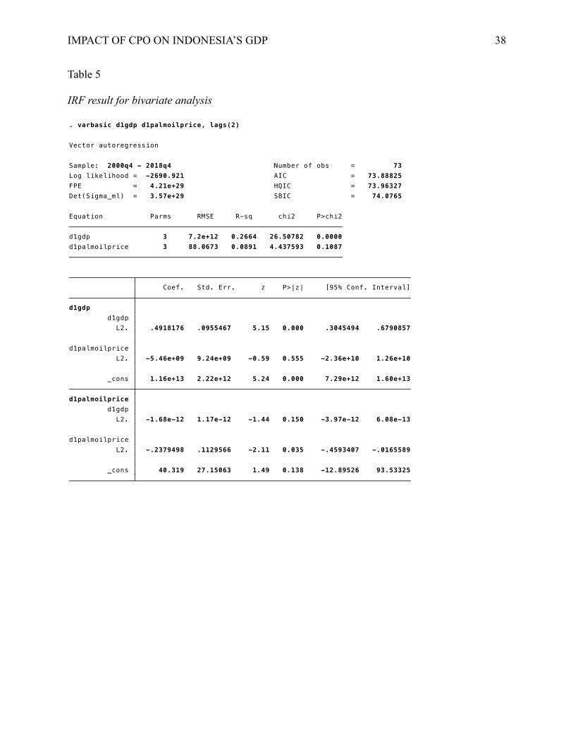
Table 5

IRF result for bivariate analysis

.

_cons 40.319 27.15063 1.49 0.138 -12.89526 93.53325 L2. -.2379498 .1129566 -2.11 0.035 -.4593407 -.0165589d1palmoilprice L2. -1.68e-12 1.17e-12 -1.44 0.150 -3.97e-12 6.08e-13 d1gdp d1palmoilprice

_cons 1.16e+13 2.22e+12 5.24 0.000 7.29e+12 1.60e+13 L2. -5.46e+09 9.24e+09 -0.59 0.555 -2.36e+10 1.26e+10d1palmoilprice L2. .4918176 .0955467 5.15 0.000 .3045494 .6790857 d1gdp d1gdp


d1palmoilprice 3 88.0673 0.0891 4.437593 0.1087d1gdp 3 7.2e+12 0.2664 26.50782 0.0000




. varbasic d1gdp d1palmoilprice, lags(2)




. varbasic d1lgdp d1lprice d1lprod lexport, lags (4)

_cons -.0368899 .0420912 -0.88 0.381 -.1193872 .0456074 L3. -.1057048 .1149282 -0.92 0.358 -.3309599 .1195504 d1lprice L3. 3.841543 3.039963 1.26 0.206 -2.116674 9.79976 d1lgdp d1lprice

_cons .0122703 .0012883 9.52 0.000 .0097452 .0147954 L3. .0028925 .0035177 0.82 0.411 -.0040022 .0097871 d1lprice L3. .0338657 .0930475 0.36 0.716 -.1485041 .2162356 d1lgdp d1lgdp


d1lprice 3 .135996 0.0314 2.332789 0.3115d1lgdp 3 .004163 0.0115 .8404727 0.6569




. varbasic d1lgdp d1lprice, lags(3)


Table 6

IRF result for multivariate analysis



_cons 2309109 493351.4 4.68 0.000 1342158 3276060 L4. .2827281 .1284865 2.20 0.028 .0308991 .534557CPOExportVolume L4. .0177913 .0855564 0.21 0.835 -.1498962 .1854789 d1prod L4. 314.5831 709.6736 0.44 0.658 -1076.352 1705.518 d1palmoilprice L4. -3.92e-08 1.65e-08 -2.37 0.018 -7.16e-08 -6.73e-09 d1gdp CPOExportVolume

_cons 1272531 814797.7 1.56 0.118 -324442.9 2869505 L4. -.2088845 .2122028 -0.98 0.325 -.6247943 .2070253CPOExportVolume L4. .3723397 .1413013 2.64 0.008 .0953943 .6492852 d1prod L4. 424.8039 1172.066 0.36 0.717 -1872.403 2722.011 d1palmoilprice L4. -3.32e-08 2.73e-08 -1.21 0.225 -8.68e-08 2.04e-08 d1gdp d1prod

_cons -49.55435 112.0077 -0.44 0.658 -269.0854 169.9767 L4. 9.12e-06 .0000292 0.31 0.755 -.0000481 .0000663CPOExportVolume L4. .0000208 .0000194 1.07 0.283 -.0000172 .0000589 d1prod L4. .0535914 .1611202 0.33 0.739 -.2621985 .3693813 d1palmoilprice L4. 1.29e-12 3.76e-12 0.34 0.731 -6.07e-12 8.65e-12 d1gdp d1palmoilprice

_cons 1.12e+13 4.22e+12 2.65 0.008 2.91e+12 1.95e+13 L4. -57550.7 1100013 -0.05 0.958 -2213537 2098436CPOExportVolume L4. 587915.2 732475.2 0.80 0.422 -847710 2023540 d1prod L4. -1.45e+10 6.08e+09 -2.39 0.017 -2.64e+10 -2.60e+09 d1palmoilprice L4. .5911261 .1416766 4.17 0.000 .3134451 .868807 d1gdp d1gdp


CPOExportVolume 5 517205 0.2229 12.33445 0.0150d1prod 5 854194 0.1948 10.40484 0.0341d1palmoilprice 5 117.423 0.0361 1.512762 0.8244d1gdp 5 4.4e+12 0.2997 18.40419 0.0010




. varbasic d1gdp d1palmoilprice d1prod CPOExportVolume, lags(4)

.

_cons 11.27598 2.005053 5.62 0.000 7.346147 15.20581 L4. .2296142 .139094 1.65 0.099 -.0430051 .5022335 lexport L4. .0818565 .296241 0.28 0.782 -.4987652 .6624781 d1lprod L4. .1454677 .3735727 0.39 0.697 -.5867214 .8776568 d1lprice L4. -13.85493 20.68828 -0.67 0.503 -54.40321 26.69336 d1lgdp lexport

_cons .5870696 .9314072 0.63 0.528 -1.238455 2.412594 L4. -.0270418 .0646133 -0.42 0.676 -.1536816 .0995981 lexport L4. .3488808 .1376128 2.54 0.011 .0791647 .618597 d1lprod L4. .098548 .1735357 0.57 0.570 -.2415757 .4386718 d1lprice L4. -13.6847 9.610326 -1.42 0.154 -32.52059 5.151196 d1lgdp d1lprod

_cons -.6624898 .9567114 -0.69 0.489 -2.53761 1.21263 L4. .0275497 .0663687 0.42 0.678 -.1025307 .15763 lexport L4. .1848411 .1413514 1.31 0.191 -.0922026 .4618848 d1lprod L4. -.142369 .1782503 -0.80 0.424 -.4917331 .2069952 d1lprice L4. 19.68092 9.871417 1.99 0.046 .3332952 39.02854 d1lgdp d1lprice

_cons .013486 .0171112 0.79 0.431 -.0200514 .0470233 L4. -.0004286 .001187 -0.36 0.718 -.0027551 .0018979 lexport L4. .0012413 .0025281 0.49 0.623 -.0037138 .0061963 d1lprod L4. -.0042634 .0031881 -1.34 0.181 -.0105119 .0019851 d1lprice L4. .4458871 .1765545 2.53 0.012 .0998466 .7919276 d1lgdp d1lgdp


lexport 5 .318026 0.0745 3.460609 0.4839d1lprod 5 .147732 0.2029 10.94805 0.0272d1lprice 5 .151746 0.1081 5.21158 0.2663d1lgdp 5 .002714 0.1317 6.522046 0.1634




. varbasic d1lgdp d1lprice d1lprod lexport, lags (4)

impact of cpo on indonesia’s gdp 2000-2018 1 ......impact of cpo on indonesia’s gdp 2000-2018 1...

Documents