impact of climate change mitigation on ocean acidi cation ... · pdf file14.1 introduction ......

OUP CORRECTED PROOF – FINAL, 08/11/2011, SPi

272

CHAPTER 14

Impact of climate change mitigation on ocean acidi! cation projections F ortunat J oos, T homas L . F rölicher, M arco S teinacher, and G ian- K asper P lattner

14.1 Introduction

Ocean acidi! cation caused by the uptake of carbon dioxide (CO 2 ) by the ocean is an important global change problem ( Kleypas et al. 1999 ; Caldeira and Wickett 2003 ; Doney et al. 2009). Ongoing ocean acidi-! cation is closely linked to global warming, as acidi! -cation and warming are primarily caused by continued anthropogenic emissions of CO 2 from fossil fuel burn-ing ( Marland et al. 2008 ), land use, and land-use change (Strassmann et al. 2007). Future ocean acidi! -cation will be determined by past and future emis-sions of CO 2 and their redistribution within the earth system and the ocean. Calculation of the potential range of ocean acidi! cation requires consideration of both a plausible range of emissions scenarios and uncertainties in earth system responses, preferably by using results from multiple scenarios and models.

The goal of this chapter is to map out the spatio-temporal evolution of ocean acidi! cation for differ-ent metrics and for a wide range of multigas climate change emissions scenarios from the integrated assessment models ( Nakic"enovic" 2000 ; Van Vuuren et al. 2008b ). By including emissions reduction sce-narios that are among the most stringent in the cur-rent literature, this chapter explores the potential bene! ts of climate mitigation actions in terms of how much ocean acidi! cation can be avoided and how much is likely to remain as a result of inertia within the energy and climate systems. The long-term impacts of carbon emissions are addressed using so-called zero-emissions commitment scenar-ios and pathways leading to stabilization of atmos-pheric CO 2 . Discussion will primarily rely on results from the cost-ef! cient Bern2.5CC model (Plattner

et al. 2008) and the comprehensive carbon cycle–climate model of the National Centre for Atmospheric Research (NCAR), CSM1.4-carbon ( Steinacher et al. 2009 ; Frölicher and Joos 2010 ).

The magnitude of the human perturbation of the climate system is well documented by observations ( Solomon et al. 2007 ). Carbon emissions from human activities force the atmospheric composition, cli-mate, and the geochemical state of the ocean towards conditions that are unique for at least the last million years (see Chapter 2 ). The current atmospheric CO 2 concentration of 390 ppmv is well above the natural range of 172 to 300 ppmv of the past 800 000 years ( Lüthi et al. 2008 ). The rate of increase in CO 2 and in the radiative forcing from the combination of the well-mixed greenhouse gases CO 2 , methane (CH 4 ), and nitrous oxide (N 2 O) is larger during the Industrial Era than during any comparable period of at least the past 16 000 years ( Joos and Spahni 2008 ). Ocean measurements over recent decades show that the increase in surface-ocean CO 2 is being paralleled by a decrease in pH (Doney et al. 2009). Ongoing global warming is unequivocal ( Solomon et al. 2007 ): observational data show that global-mean sea level is rising, ocean heat content increas-ing, Arctic sea ice retreating, atmospheric water vapour content increasing, and precipitation pat-terns changing. The last decade (2000 to 2009) was, on a global average, the warmest in the instrumental record (http://data.giss.nasa.gov/gistemp/). Proxy reconstructions suggest that recent anthropogenic in# uences have widened the last-millennium multi-decadal temperature range by 75% and that late 20th century warmth exceeded peak temperatures over the past millennium by 0.3°C ( Frank et al. 2010 ).


CLIMATE CHANGE MIT IGATION AND OCEAN ACIDIF ICATION PROJECTIONS 273

The range of plausible 21st century emissions pathways leads to further global warming and ocean acidi! cation ( Van Vuuren et al. 2008b ; Strassmann et al. 2009 ). Projections based on the sce-narios of the Special Report on Emissions Scenarios (SRES) of the Intergovernmental Panel on Climate Change (IPCC) give reductions in average global surface pH of between 0.14 and 0.35 units over the 21st century, adding to the present decrease of 0.1 units since pre-industrial time (Orr et al. 2005; see also Chapters 1 and 3). Comprehensive earth sys-tem model simulations show that continued carbon emissions over the 21st century will cause irrevers-ible climate change on centennial to millennial timescales in most regions, and impacts related to ocean acidi! cation and sea level rise will continue to aggravate for centuries even if emissions are stopped by the year 2100 (Frölicher and Joos 2010 ). In contrast, in the absence of future anthropogenic emissions of CO 2 and other radiative agents, forced changes in surface temperature and precipitation will become smaller in the next centuries than inter-nal variability for most land and ocean grid cells and ocean acidi! cation will remain limited. This demonstrates that effective measures to reduce anthropogenic emissions can make a difference. However, continued carbon emissions will affect climate and the ocean over the next millennium and beyond (Archer et al. 1999; Plattner et al. 2008) and related climate and biogeochemical impacts pose a substantial threat to human society.

Thirty years ago, with their box-diffusion carbon cycle model, Siegenthaler and Oeschger (1978) dem-onstrated the long lifetime of an atmospheric CO 2 perturbation and pointed out that carbon emissions must be reduced ‘if the atmospheric radiation bal-ance is not to be disturbed in a dangerous way’. The United Nations Framework Convention on Climate Change (UNFCCC) that came into force in 1994 has the ultimate objective (article 2) ‘to achieve . . . stabi-lization of greenhouse gas concentrations in the atmosphere at a level that would prevent dangerous anthropogenic interference with the climate system. Such a level should be achieved within a time frame suf! cient to allow ecosystems to adapt naturally to climate change . . .’ ( UN 1992 ). Scenarios provide a useful framework for establishing policy-relevant information related to the UNFCCC. Here, the link

between atmospheric CO 2 level and ocean acidi! ca-tion, and the timescales of change, are addressed.

The outline of this chapter is as follows. In the next section, we will discuss different classes of sce-narios, their underlying assumptions, and how these scenarios are used. Metrics for assessing ocean acidi! cation are also introduced. In Section 14.3, the evolution over this century of atmospheric CO 2 , global-mean surface air temperature, and global-mean surface ocean acidi! cation for the recent range of baseline and mitigation scenarios from integrated assessment models is presented. In Section 14.4, the minimum commitment, as a result of past and 21st century emissions, to long-term cli-mate change and ocean acidi! cation arising from inertia in the earth system alone is addressed. In Section 14.5, regional changes in surface ocean chemistry are discussed. In Section 14.6, delayed responses, irreversibility, and changes in the deep ocean are addressed using results from the compre-hensive NCAR CSM1.4-carbon model. Finally, in Section 14.7, idealized pro! les leading to CO 2 stabi-lization are discussed to further highlight the link between greenhouse gas stabilization, climate change, and ocean acidi! cation. The overarching logic is to use the cost-ef! cient Bern2.5CC model to explore the scenario space and uncertainties for global-mean values and the NCAR CSM1.4-carbon model to investigate regional details for a limited set of scenarios. The set of baseline and emissions scenarios and associated changes in CO 2 and glo-bal-mean surface temperature have been previously discussed ( Van Vuuren et al. 2008b ; Strassmann et al. 2009 ). We also refer to the literature for a more detailed discussion of the NCAR CSM1.4-carbon ocean acidi! cation results ( Steinacher et al. 2009 ; Frölicher and Joos 2010 ).

14.2 Scenarios and metrics

Scenario-based projections are a scienti! c tool kit for investigating alternative evolutions of anthro-pogenic emissions and their in# uence on climate, the earth system, and the socio-economic system. Scenario-based projections are not to be misunder-stood as predictions of the future, and as the time horizon increases the basis for the underlying assumptions becomes increasingly uncertain.


274 OCEAN ACIDIF ICATION

One class of scenarios includes idealized emis-sions or concentration pathways to investigate processes, feedbacks, timescales, and inertia in the climate system. These scenarios are usually devel-oped from a natural science perspective and used for their illustrative power. Examples are a com-plete instantaneous reduction of emissions at a given year or idealized pathways leading to stabili-zation of greenhouse gas concentrations ( Schimel et al. 1997 ). Another class of emissions scenarios has been developed using integrated assessment frame-works and integrated assessment models (IAMs) by considering plausible future demographic, social, economic, technological, and environmental devel-opments. Examples include the scenarios of the IPCC SRES ( Nakic"enovic" et al. 2000 ) and the more recently developed representative concentration pathways (RCPs; Moss et al. 2008 , 2010 ; Van Vuuren et al. 2008a ).

The SRES emissions scenarios do not include explicit climate change mitigation actions. Such sce-narios are usually called baseline or reference sce-narios. In this chapter, results based on the two illustrative SRES scenarios B1 and A2, a low- and a high-emissions baseline scenario, are discussed ( Fig. 14.1 ). The SRES scenarios have been widely

used in the literature and in the IPCC Fourth Assessment Report. They are internally consistent scenarios in the sense that each is based on a ‘narra-tive storyline’ that describes the relationships between the forces driving emissions. The 21st cen-tury emissions of the major anthropogenic green-house gases [CO 2 , CH 4 , N 2 O, halocarbons, and sulphur hexa# uoride (SF 6 )], aerosols and tropo-spheric ozone precursors [sulphur dioxide (SO 2 ), carbon monoxide (CO), NO x , and volatile organic compounds (VOCs)] are quanti! ed with IAMs. The extent of the technological improvements contained in the SRES scenarios is not always appreciated. The SRES scenarios include already large and important improvements in energy intensity (energy used per unit of gross domestic product) and the deployment of non-carbon-emitting energy supply technologies compared with the present (Edmonds et al. 2004). By the year 2100, the primary energy demand in the SRES scenarios ranges from 55% to more than 90% lower than had no improvement in energy intensity occurred. In addition, in many of the SRES scenarios the deploy-ment of non-carbon-emitting energy supply sys-tems (solar, wind, nuclear, and biomass) exceeds the size of the global energy system in 1990.

Figure 14.1 Cumulative CO 2 emissions in gigatonnes of carbon (Gt C) over the 21st century for a range of baseline (B; red), climate mitigation (blue), and the SRES A2 and B1 (black) scenarios. The numbers related to the mitigation scenarios indicate the radiative forcing targets in W m –2 imposed in the IAMs. The labels below the columns refer to the IAMs used to quantify the scenarios (Weyant et al. 2006) and to the SRES scenarios ( Nakicenovic 2000 ), respectively.

Cum

ulat

ive

carb

on e

mis

sion

s [G

t C]

2100

1800

1500

1200

900

0AIM IPAC IMAGE MiniCam EPPA MESSAGE SRES

600

300

B

B

BB

B

B(a)

4.54.5

4.54.5

4.54.5

4.5

5.3

3.7

2.9

4.0

3.2

B(b)

2.6

3.5

A2

B1

4.5



However, by design they do not include explicit policies to mitigate greenhouse gas emissions, which would lower the extent of climate change experienced over the 21st century.

Progress in developing multigas mitigation sce-narios after the SRES report now allows for a com-parison between consequences for the earth system of climate mitigation versus baseline scenarios. Figure 14.1 illustrates the relationship between sce-narios and individual IAMs and how individual mitigation scenarios are linked to a speci! c baseline scenario for the post-SRES set of scenarios. Many mitigation scenarios were generated with several IAMs as part of the Energy Modeling Forum Project 21 (EMF-21; Weyant et al. 2006). The IAMs feature representations of the energy system and other parts of the economy, such as trade and agriculture, with varying levels of spatial and process detail. They also include formulations to translate emis-sions into concentrations and the associated radia-tive forcing (RF). The latter is a metric for the perturbation of the radiative balance of the lower atmosphere–surface system. Scenarios are gener-ated by minimizing the total costs under the con-straints set by societal drivers (e.g. population, welfare, and technological innovation) and most are related to SRES ‘storylines’. Adding a constraint on RF in a baseline scenario leads to a scenario with policies speci! cally aimed at mitigation. The miti-gation scenarios analysed here are constrained by stabilization of total RF in the period 2100 to 2150 with RF targets ranging from 2.6 to 5.3 W m –2 . From the wider set of baseline and mitigation scenarios described in the literature, four have been speci! -cally selected and termed representative concentra-tion pathways (RCPs). These include two mitigation scenarios with a RF target of 2.6 and 4.5 W m –2 and two baseline scenarios with a RF of around 6 and 8.5 W m –2 by the end of this century.

Two metrics appear particularly well suited for characterizing the outcome of a scenario in terms of ocean acidi! cation. These are changes in pH and changes in the saturation state of water with respect to aragonite, a mineral form of calcium carbonate (CaCO 3 ) secreted by marine organisms. Ocean uptake of the weak acid CO 2 from the atmosphere causes a reduction in pH and in turn alters the CaCO 3 precipitation equilibrium (see Chapter 1 ).

Recent studies indicate that ocean acidi! cation due to the uptake of CO 2 has adverse consequences for many marine organisms as a result of decreased CaCO 3 saturation, affecting calci! cation rates, and via disturbance to acid–base physiology (see Chapters 6–8). Vulnerable organisms that build shells and other structures of CaCO 3 in the rela-tively soluble form of aragonite or high-magnesian calcite, but also organisms that form CaCO 3 in the more stable form of calcite may be affected. Undersaturation as projected for the high-latitude ocean (Orr et al. 2005; Steinacher et al. 2009 ) has been found to affect pteropods for example, an abundant group of species forming aragonite shells (Orr et al. 2005; Comeau et al. 2009). Changes in CaCO 3 satura-tion are also thought to affect coral reefs ( Kleypas et al. 1999 ; Langdon and Atkinson 2005 ; Hoegh-Guldberg et al. 2007; Cohen and Holcomb 2009 ). The impacts are probably not restricted to ecosys-tems at the ocean surface, but potentially also affect life in the deep ocean such as the extended deep-water coral systems and ecosystems at the ocean # oor. The degree of sensitivity varies among species ( Langer et al. 2006 ; Müller et al. 2010 ) and there is a debate about whether some taxa may show enhanced calci! cation at the levels of CO 2 projected to occur over the 21st century (Iglesias-Rodriguez et al. 2008). This wide range of different responses is expected to affect competition among species, eco-system structure, and overall community produc-tion of organic material and CaCO 3 . On the other hand, the impact of plausible changes in CaCO 3 production and export (Gangstø et al. 2008) on atmospheric CO 2 is estimated to be small ( Heinze 2004 ; Gehlen et al. 2007). Other impacts of ocean acidi! cation with potential in# uences on marine ecosystems include alteration in the speciation of trace metals as well as an increase in the transpar-ency of the ocean to sound (Hester et al. 2008). The changes in the chemical composition of seawater such as higher concentrations of dissolved CO 2 are also likely to affect the coupled carbon and nitrogen cycle and the food web in profound ways (Hutchins et al. 2009), and the volume of water with a ratio of oxygen to CO 2 below the threshold for aerobic life is likely to expand (Brewer and Peltzer 2009 ).

The saturation state with respect to aragonite, $ a , is de! ned by:



2 23

asp

[Ca ][CO ]*

+ -

W =K

where brackets denote concentrations in seawater, here for calcium ions and carbonate ions, and K * sp is the apparent solubility product de! ned by the equi-librium relationship for the dissolution reaction of aragonite. Similarly, saturation can be de! ned with respect to calcite which is less soluble than arago-nite. Uptake of CO 2 causes an increase in total dis-solved inorganic carbon ( C T ) and a decrease in the carbonate ion concentration and in saturation (see Chapter 1 ). Shells or other structures start to dis-solve in the absence of protective mechanisms when saturation falls below 1 for the appropriate mineral phase. A value of $ greater than 1 corresponds to supersaturation. Supersaturated conditions are pos-sible, as the activation energy for forming aragonite or calcite is high.

The pH describes the concentration or, more pre-cisely, the activity of the hydrogen ion in water, a H , by a logarithmic function:

T 10 HpH log .+= - a

The activity of hydrogen ion is important for all acid–base reactions. In this chapter, the total pH scale is used as indicated by the subscript T.

14.3 Baseline and mitigation emissions scenarios for the 21st century: how much acidi! cation can be avoided?

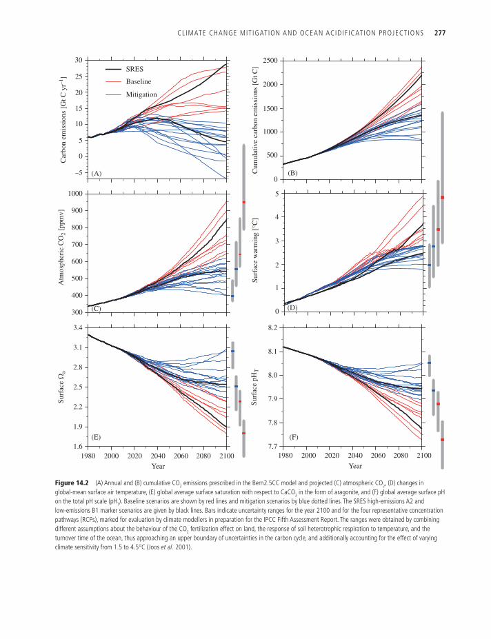
Figure 14.1 shows the cumulative carbon emissions over this century for the recent set of baseline and mitigation scenarios ( Van Vuuren et al. 2008b ) and Fig. 14.2 their temporal evolution. Cumulative CO 2 emissions are in the range of 1170 to 1930 Gt C for the seven baseline scenarios and between 370 and 1140 Gt C for the mitigation scenarios, with the highest emissions associated with a high forcing and a weak mitigation target. In the baseline (no cli-mate policy) scenarios, the range of increase in greenhouse gas emissions by 2100 is from 70 to almost 250% compared with the year 2000 (here, emissions are measured in CO 2 -equivalent—CO 2 -equivalent emissions of a forcing agent denote the

amount of CO 2 emissions that would cause the same radiative forcing over a time period of 100 years; IPCC 2007 ). Emissions growth slows down in the second half of the century in all baseline scenar-ios, because of a combination of stabilizing global population levels and continued technological change. The mitigation scenarios necessarily follow a different path, with a peak in global emissions between 2020 and 2040 at a maximum value of 50% above current emissions.

The projected CO 2 concentrations for the baseline cases calculated with the Bern2.5CC model (Plattner et al. 2008) range from 650 to 960 ppmv in 2100 using best-estimate model parameters ( Fig. 14.2C ). The CO 2 concentrations in the mitigation scenarios range from 400 to 620 ppmv in 2100. Uncertainties in the carbon cycle and climate sensitivity increase the overall range to 370 to 1310 ppmv (bars in Fig. 14.2C ; Plattner et al. 2008). Uncertainties are particu-larly large for the high end. The two scenario sets, baseline and mitigation, are also distinct with respect to their trends. All baseline scenarios show an increasing trend in atmospheric CO 2 , implying rising concentrations beyond 2100. In contrast, the mitigation scenarios show little growth or even a declining trend in CO 2 by 2100.

Projected global-mean surface air temperature changes by the year 2100 (relative to 2000) are 2.4 to 4.2°C ( Fig. 14.2D ) for the baseline scenarios and best-estimate Bern2.5CC model parameters. Uncertainties in the carbon cycle and climate sensi-tivity more than double the ranges associated with emissions. For the mitigation scenarios, the pro-jected temperature changes by 2100 are 1.1 to 2.1°C using central model parameters. The mitigation sce-narios bring down the overall range of CO 2 and temperature change substantially relative to the baseline range. As for CO 2 , the greatest difference compared with the baseline is seen during the sec-ond part of the century, when the rate of tempera-ture change slows considerably in all mitigation scenarios in contrast to the baseline scenarios. In several mitigation scenarios, surface air tempera-ture has more or less stabilized by year 2100 ( Van Vuuren et al. 2008b ; Strassmann et al. 2009 ).

The evolution of the global-mean saturation state of aragonite ( Fig. 14.2E ) and pH T ( Fig. 14.2F ) in the surface ocean mirrors the evolution of atmospheric



Figure 14.2 (A) Annual and (B) cumulative CO 2 emissions prescribed in the Bern2.5CC model and projected (C) atmospheric CO 2 , (D) changes in global-mean surface air temperature, (E) global average surface saturation with respect to CaCO 3 in the form of aragonite, and (F) global average surface pH on the total pH scale (pH T ). Baseline scenarios are shown by red lines and mitigation scenarios by blue dotted lines. The SRES high-emissions A2 and low-emissions B1 marker scenarios are given by black lines. Bars indicate uncertainty ranges for the year 2100 and for the four representative concentration pathways (RCPs), marked for evaluation by climate modellers in preparation for the IPCC Fifth Assessment Report. The ranges were obtained by combining different assumptions about the behaviour of the CO 2 fertilization effect on land, the response of soil heterotrophic respiration to temperature, and the turnover time of the ocean, thus approaching an upper boundary of uncertainties in the carbon cycle, and additionally accounting for the effect of varying climate sensitivity from 1.5 to 4.5°C ( Joos et al. 2001 ).

1980 2000 2020 2040 2060 2080 2100Year

Cum

ulat

ive

carb

on e

mis

sion

s [G

t C]

2500

2000

1500

1000

500

0(B)

Atm

osph

eric

CO

2 [p

pmv]

1000

900

800

700

600

500

400

300 (C)

Surf

ace

war

min

g [°

C]

(D)

3

2

0

4

5

1

Surf

ace W

a

3.4

3.1

2.8

2.5

2.2

1.9

1.6(E)

1980 2000 2020 2040 2060 2080 2100Year

SRES

Baseline

Mitigation

(A)

Car

bon

emis

sion

s [G

t C y

r–1]

30

25

20

15

10

0

–5

5

Surf

ace

pHT

8.2

8.1

8.0

7.9

7.8

7.7(F)



CO 2 . $ a decreases from a pre-industrial value of 3.7 to between 2.3 and 1.8 for the baseline scenarios and to between 3.1 and 2.4 for the mitigation scenarios using the standard model parameters. Again, uncer-tainties in the projections associated with the car-bon cycle and climate sensitivity are largest for the high-emissions scenarios and lower-bound pro-jected $ a becomes as low as a global average of 1.4 for the reference scenario with the highest emis-sions. Global average surface pH T decreases from a pre-industrial value of 8.18 to 7.88–7.73 for the base-line scenarios and to 8.05–7.90 for the mitigation scenarios, with a lower bound value for the most extreme scenario of 7.6. The uncertainty ranges for $ a and pH T stem almost entirely from uncertainties in the projection of atmospheric CO 2 as carbonate chemistry parameters are well de! ned and surface-water CO 2 follows the atmospheric rise relatively closely. Trends in surface saturation and pH T are strongly declining in 2100 for the baseline scenarios, whereas the mitigation scenarios show small or even increasing trends.

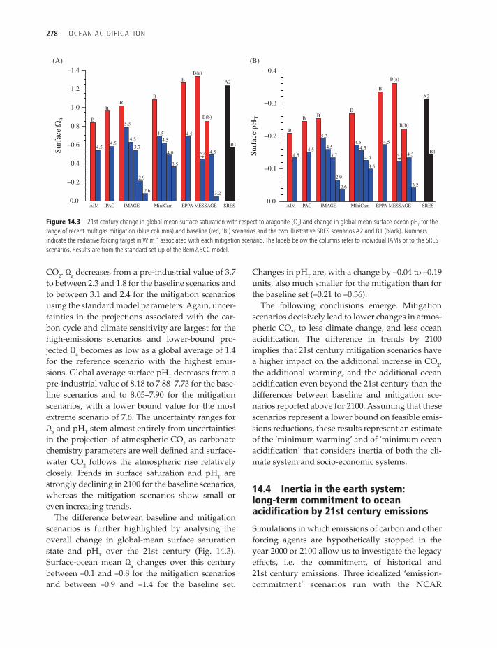
The difference between baseline and mitigation scenarios is further highlighted by analysing the overall change in global-mean surface saturation state and pH T over the 21st century ( Fig. 14.3 ). Surface-ocean mean $ a changes over this century between –0.1 and –0.8 for the mitigation scenarios and between –0.9 and –1.4 for the baseline set.

Changes in pH T are, with a change by –0.04 to –0.19 units, also much smaller for the mitigation than for the baseline set (–0.21 to –0.36).

The following conclusions emerge. Mitigation scenarios decisively lead to lower changes in atmos-pheric CO 2 , to less climate change, and less ocean acidi! cation. The difference in trends by 2100 implies that 21st century mitigation scenarios have a higher impact on the additional increase in CO 2 , the additional warming, and the additional ocean acidi! cation even beyond the 21st century than the differences between baseline and mitigation sce-narios reported above for 2100. Assuming that these scenarios represent a lower bound on feasible emis-sions reductions, these results represent an estimate of the ‘minimum warming’ and of ‘minimum ocean acidi! cation’ that considers inertia of both the cli-mate system and socio-economic systems.

14.4 Inertia in the earth system: long-term commitment to ocean acidi! cation by 21st century emissions

Simulations in which emissions of carbon and other forcing agents are hypothetically stopped in the year 2000 or 2100 allow us to investigate the legacy effects, i.e. the commitment, of historical and 21st century emissions. Three idealized ‘emission- commitment’ scenarios run with the NCAR

Figure 14.3 21st century change in global-mean surface saturation with respect to aragonite (! a ) and change in global-mean surface-ocean pH T for the range of recent multigas mitigation (blue columns) and baseline (red, ‘B’) scenarios and the two illustrative SRES scenarios A2 and B1 (black). Numbers indicate the radiative forcing target in W m –2 associated with each mitigation scenario. The labels below the columns refer to individual IAMs or to the SRES scenarios. Results are from the standard set-up of the Bern2.5CC model.

Surf

ace W

a

–1.4

–1.2

–1.0

–0.8

–0.6

0.0

–0.4

–0.2

AIM IPAC IMAGE MiniCam EPPA MESSAGE SRES

B

B

BB

BB(a)

4.54.5

4.54.5 4.5

4.5

4.5

4.5

5.3

3.7

2.9

2.6

4.0

3.5

3.2

B(b)

A2

B1

(A)

Surf

ace

pHT

–0.4

–0.3

–0.2

–0.1

0.0AIM IPAC IMAGE MIniCam EPPA MESSAGE SRES

B

B

BB

B

B(a)

4.54.5 4.5

4.5 4.5

4.5

4.54.5

5.3

3.7

2.9

2.6

4.0

3.5

3.2

B(b)

A2

B1

(B)



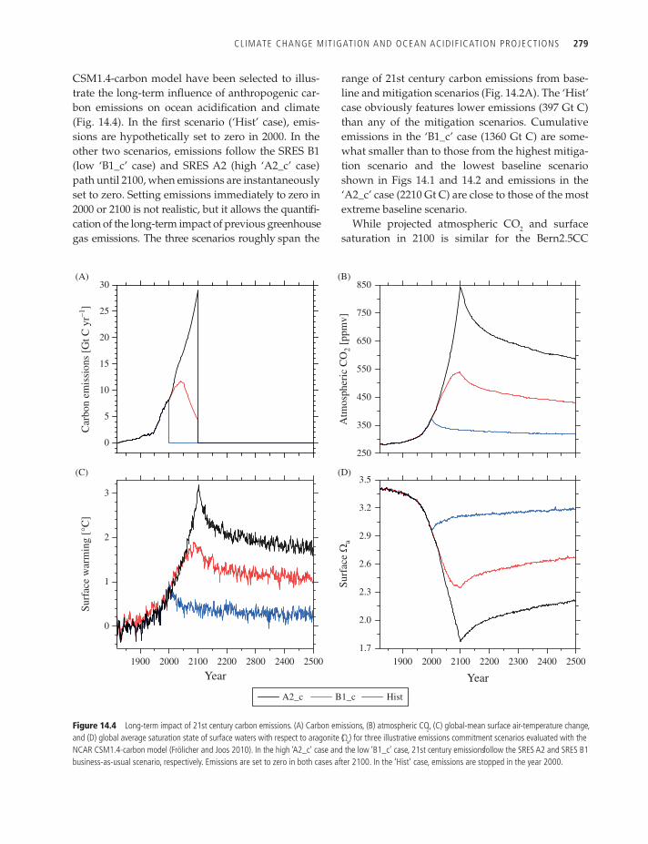
CSM1.4-carbon model have been selected to illus-trate the long-term in# uence of anthropogenic car-bon emissions on ocean acidi! cation and climate ( Fig. 14.4 ). In the ! rst scenario (‘Hist’ case), emis-sions are hypothetically set to zero in 2000. In the other two scenarios, emissions follow the SRES B1 (low ‘B1_c’ case) and SRES A2 (high ‘A2_c’ case) path until 2100, when emissions are instantaneously set to zero. Setting emissions immediately to zero in 2000 or 2100 is not realistic, but it allows the quanti! -cation of the long-term impact of previous greenhouse gas emissions. The three scenarios roughly span the

range of 21st century carbon emissions from base-line and mitigation scenarios ( Fig. 14.2A ). The ‘Hist’ case obviously features lower emissions (397 Gt C) than any of the mitigation scenarios. Cumulative emissions in the ‘B1_c’ case (1360 Gt C) are some-what smaller than to those from the highest mitiga-tion scenario and the lowest baseline scenario shown in Figs 14.1 and 14.2 and emissions in the ‘A2_c’ case (2210 Gt C) are close to those of the most extreme baseline scenario.

While projected atmospheric CO 2 and surface saturation in 2100 is similar for the Bern2.5CC

Figure 14.4 Long-term impact of 21st century carbon emissions. (A) Carbon emissions, (B) atmospheric CO 2 , (C) global-mean surface air-temperature change, and (D) global average saturation state of surface waters with respect to aragonite (! a ) for three illustrative emissions commitment scenarios evaluated with the NCAR CSM1.4-carbon model (Frölicher and Joos 2010 ). In the high ‘A2_c’ case and the low ‘B1_c’ case, 21st century emissions follow the SRES A2 and SRES B1 business-as-usual scenario, respectively. Emissions are set to zero in both cases after 2100. In the ‘Hist’ case, emissions are stopped in the year 2000.

850

750

650

550

450

350

250

Surf

ace

war

min

g [°

C]

3

2

1

0

Surf

ace W

aA

tmos

pher

ic C

O2

[ppm

v]

1900 2000 2100 2200 2800 2400 2500

Year

3.5

3.2

2.9

2.6

2.3

2.0

1.71900 2000 2100 2200 2300 2400 2500

Year

Car

bon

emis

sion

s [G

t C y

r–1]

30

25

20

15

10

0

5

(A) (B)

(C) (D)

A2_c B1_c Hist



model ( Fig. 14.2C ) and the CSM1.4-carbon ( Fig. 14.4B ), projected 21st century warming is lower in CSM1.4-carbon than in the Bern2.5CC model. This difference is primarily related to the difference in climate sensitivity; 2°C for a nominal doubling of CO 2 in the CSM1.4 versus 3.2°C for the Bern2.5CC best estimate.

Atmospheric CO 2 concentration increases by 300% and by 190% over this century in the high ‘A2_c’ and low ‘B1_c’ case, respectively ( Fig. 14.4B ). Thereafter, atmospheric CO 2 decreases only very slowly, although carbon emissions are (unrealisti-cally) reduced to zero in 2100. Atmospheric CO 2 concentration is still twice as high by 2500 than in pre-industrial times in the ‘A2_c’ case. On the other hand, CO 2 falls below 350 ppmv within a few dec-ades in the ‘Hist’ case. The global-mean surface temperature anomaly peaks at 3°C in the ‘A2_c’ case and at 1.7°C in the ‘B1_c’ case and remains elevated for centuries ( Fig. 14.4C ). In the ‘Hist’ case, global-mean surface temperature remains only slightly perturbed (0.2°C warming) by 2500. The global average saturation state of aragonite in the surface ocean closely follows the evolution of atmospheric CO 2 . Mean surface $ a is reduced by about half in 2100 for the ‘A2_c’ case and remains reduced over the next centuries.

The long perturbation lifetime of CO 2 is a conse-quence of the centennial to millennial timescales of overturning of various carbon reservoirs. Most of the excess carbon is taken up by the ocean and slowly (on a multicentury to millennial timescale) mixed down to the abyss. Ultimately, interaction with ocean sediments and the weathering cycle will remove the anthropogenic carbon perturba-tion from the atmosphere on timescales of millen-nia to hundreds of millennia (Archer et al. 1999; see Chapter 2 ).

In conclusion, the results from the commitment scenarios show that the magnitude of 21st century CO 2 emissions pre-determines the range of atmos-pheric CO 2 concentrations, temperature, and ocean acidi! cation for the coming centuries, at least in the absence of the large-scale deployment of a technology to remove excess CO 2 from the atmosphere. In other words, the CO 2 emitted in the next decades will per-turb the physical climate system, biogeochemical cycle, and ecosystems for centuries.

14.5 Regional changes in surface ocean acidi! cation: undersaturation in the Arctic is imminent

The impacts of climate change and ocean acidi! ca-tion on natural and socio-economic systems depend on local and regional changes in climate and acidi! -cation rather than on global average metrics. It is important to recognize that the global-mean metrics discussed in the previous sections lead to different changes regionally ( Fig. 14.5 ). Fortunately, the spa-tial patterns of change in pH T and surface $ a scale closely with atmospheric CO 2 ( Figs 14.6 and 14.7 ). This eases the discussion of local changes for the scenario range and enables us to make inferences for local and regional changes from projected atmos-pheric CO 2 . This section presents regional changes in the saturation state of aragonite, $ a , and pH T for the three commitment scenarios introduced in the previous section and as evaluated in the NCAR CSM1.4-carbon model.

There are large regional differences in the surface saturation state for pre-industrial conditions and in its change over time ( Figs 14.5 and 14.6 ). The sur-face ocean was saturated with respect to aragonite in all regions under pre-industrial conditions ( Kleypas et al. 1999 ; Key et al. 2004 ; Steinacher et al. 2009 ); the lowest saturation levels are simulated in the Arctic and in the Southern Ocean, whereas sur-face water with saturation values above 4 can be found in the tropics.

Surface-water saturation is projected to decrease rapidly in all regions until 2100 and remains reduced for centuries for all three zero-emission commitment scenarios ( Fig. 14.6 ). The largest ocean-surface changes are found in the tropics and subtropics for $ a . In the high ‘A2_c’ case, $ a in the tropics and subtropics decreases from a satu-ration state of more than 4 in pre-industrial times to saturation below 2.5 at the end of the 21st cen-tury. The saturation of tropical and subtropical surface waters remains below 3 until 2500. Although experimental evidence remains scarce, these projected low saturation states in combina-tion with other stress factors such as increased tem-perature pose the risk of the irreversible destruction of warm-water coral reefs ( Kleypas et al. 1999 ; Hoegh-Guldberg et al. 2007).



Undersaturation in the Arctic is imminent ( Fig. 14.6C ). By the time atmospheric CO 2 exceeds 490 ppmv (in 2040 in the ‘A2_c’ case), more than half of the Arctic Ocean will be undersaturated (annual mean; Steinacher et al . 2009 ). Undersaturation with respect to aragonite remains widespread in the Arctic Ocean for centuries even after cutting emis-sions in 2100 for both the ‘A2_c’ and the ‘B1_c’ cases (Frölicher and Joos 2010 ). The Southern Ocean

becomes undersaturated on average when atmos-pheric CO 2 exceeds 580 ppmv (Orr et al. 2005) and remains undersaturated for centuries for the ‘A2_c’ commitment case. Large-scale undersaturation in the Southern Ocean is avoided in the ‘B1_c’ and ‘Hist’ cases.

The main reason for the vulnerability of the Arctic Ocean is its naturally low saturation state. In addi-tion, climate change ampli! es ocean acidi! cation in

Figure 14.5 Regional distribution of the annual-mean saturation state with respect to aragonite (! a ) in the surface ocean for (A) pre-industrial conditions (here 1820), (B) by the year 2000, (C, D) by the end of the century, and (E, F) by 2500. The NCAR CSM1.4-carbon model was forced with reconstructed CO 2 emissions up to 2000. Emissions were set to zero after 2100 in the high ‘A2_c’ case (C, E) and after 2000 in the ‘Hist’ case (D, F). Blue colours indicate undersaturation and green to red colours supersaturation.

80˚N

(A) (B)

(D)(C)

(F)(E)

40˚N

0˚

40˚S

80˚N

40˚N

0˚

40˚S

80˚N

Year 2500 (A2_c) Year 2500 (Hist)

Year 2100 (A2_c) Year 2100 (Hist)

Year 1820 Year 2000

40˚N

0˚

40˚S

50˚E 150˚E 110˚W 10˚W 50˚E 150˚E 110˚W 10˚W0

1

2

3

4

5

0

1

2

3

4

5

0

2

3

4

5Wa

1



Figure 14.6 Projected evolution of CaCO 3 saturation states (left) and total pH (right) in the surface of the tropical ocean (30°N–30°S), Southern Ocean (60°S–90°S), and Arctic Ocean (65°N–90°N, except the Labrador and Greenland–Iceland–Norwegian seas) and for emissions commitment scenarios with no (‘Hist’ case, blue line, blue shading), low (‘B1_c’ case, red line, red shading) and high (‘A2_c’ case, black line, grey shading) emissions in the 21st century. Saturation with respect to aragonite, ! a, , is indicated on the left y -axis and with respect to calcite, ! c , on the right y -axis. Shown are modelled annual means as well as the combined spatial and interannual variability of annual-mean values within each region (shading, ±1 SD). Observation-based estimates are shown by squares for the Southern Ocean and the tropics (GLODAP and World Ocean Atlas 2001, annual mean) and for summer conditions in the Arctic Ocean (CARINA database) with bars indicating the spatial variability. Model results are from the NCAR CSM1.4-carbon model. The level of ! = 1 separating supersaturated and undersaturated conditions for aragonite and calcite is shown by dashed, horizontal lines.

5

4

3

2

Wa

Wa

Wa

Wc

Wc

Wc

pHT

pHT

pHT

1

0

5

4

3

2

1

0

5

4

3

2

1

0

1800 1900 2000

Aragonite saturationCalcite saturation

2100 2200 2300 2400 2500 1800 1900 2000 2100 2200 2300 2400 2500

1800 1900 2000 2100 2200 2300 2400 2500 1800 1900 2000 2100 2200 2300 2400 2500

1800 1900 2000 2100 2200Year Year

2300 2400 25000

1

2

3

4

5

6

7

0

1

2

3

4

5

6

7

0

1

2

3

4

5

6

7Tropical Ocean (A) Tropical Ocean (D)

Southern Ocean (B) Southern Ocean (E)

Arctic Ocean (C) Arctic Ocean (F)8.3

8.2

8.1

8.0

7.9

7.8

7.7

7.6

8.3

8.2

8.1

8.0

7.9

7.8

7.7

7.6

8.3

8.2

8.1

8.0

7.9

7.8

7.7

7.6

1800 1900 2000 2100 2200 2300 2400 2500



the Arctic, in contrast to other regions such as the Southern Ocean and the low-latitude oceans, where climate change has almost no effect on the satura-tion state in our simulations. Climate change ampli-! es the projected decrease in annual-mean $ a in the Arctic Ocean by 22% mainly due to surface freshen-ing in response to the retreat of sea ice, causing local alkalinity to decrease and the uptake of anthropo-genic carbon to increase (see also Chapter 3 ).

In summary, regional changes in the saturation state and pH T of surface waters are distinct. The largest decrease in pH T is simulated in the Arctic Ocean, where the lowest saturation is also found. Undersaturation is imminent in Arctic surface water ( Figs 14.6 and 14.7 ) and remains widespread over centuries for 21st century carbon emissions of the order of 1000 Gt C or more.

14.6 Delayed responses in the deep ocean

Ocean acidi! cation also affects the ocean interior as anthropogenic carbon continues to invade the ocean. Figure 14.8 displays how the saturation state and pH T changes along the transect from Antarctica, through the Atlantic Ocean to the North Pole for the ‘A2_c’ commitment scenario. The saturation

horizon separating supersaturated from undersat-urated water rises from a depth between ~2000 and 3000 m all the way up to the surface at high lati-tudes. The volume of water that is supersaturated with respect to aragonite strongly decreases with time. In parallel, the volume of water with low pH T expands.

A general decrease in CaCO 3 saturation corre-sponds to a loss of volume providing habitat for many species that produce CaCO 3 structures. Following Steinacher et al. ( 2009 ), ! ve classes of aragonite saturation levels are de! ned: (1) $ a above 4, considered optimal for the growth of warm-water corals, (2) $ a of 3 to 4, considered as adequate for coral growth, (3) $ a of 2 to 3, (4) $ a of 1 to 2, considered marginal to inadequate for coral growth, though experimental evidence is scarce, and ! nally (5) undersaturated water considered to be unsuitable for aragonite producers. Figure 14.9 shows the evolution of the ocean volume occupied by these ! ve classes for the three com-mitment simulations. In the ‘A2_c’ case, water masses with saturation above 3 vanish by 2070 (CO 2 ~ 630 ppmv). Overall, the volume occupied by supersaturated water decreases from 40% in pre-industrial times to 25% in 2100 and 10% in 2300, and the volume of undersaturated water

Figure 14.7 Saturation state (! a ) and total pH (pH T ) in surface water of three regions as a function of atmospheric CO 2 . Results are from the low ‘B1_c’ (dashed) and high ‘A2_c’ (solid) commitment scenarios. The relation between atmospheric CO 2 and saturation state and pH T shows almost no path dependency in the tropical ocean and Southern Ocean. Some path dependency is found in the Arctic Ocean, with lower values in surface saturation and pH T for a given CO 2 concentration simulated after the peak in atmospheric CO 2 . Note that the pH T –CO 2 curves are shifted by +0.1 pH units for the tropical region and by –0.1 pH units for the Arctic region for clarity.

5

4

3

Wa

pHT

2

1

0300 400 500

Arctic Ocean

Aragonite saturation

Southern Ocean

Tropical oceanTropical ocean

(shifted by +0.1)

Atmospheric pCO2 (ppm) Atmospheric pCO2 (ppm)600 700 800 300

7.5

7.6

7.7

7.8

7.9

8.0

8.1

8.2

8.3

(A) (B)

400 500 600 700

SouthernOceanArctic Ocean

(shifted by –0.1)

800



Figure 14.8 Saturation state with respect to aragonite (! a , left) and total pH (pH T , right) in the Atlantic and Arctic Oceans (zonal mean) for the high ‘A2_c’ commitment scenario by the year 1820 (A, E), 2100 (B, F), 2300 (C, G), and 2500 (D, H). Blue colours in the left panels indicate undersaturation. Note the different depth scales for the upper and the deep ocean, separated by the white horizontal line.

0 5Wa pHT

8.3

8.0

7.7

7.4

7.1

8.3

8.0

7.7

7.4

7.1

8.3

8.0

7.7

7.4

7.1

7.1

8.3

8.0

7.7

7.4

4

3

2

1

0

5

4

3

2

1

0

5

4

3

2

1

0

5

4

3

2

1

0

200

400

600

800

1000

2000

3000

4000

5000

040˚S 40˚N 80˚N

1820 (A) 1820 (E)

2100 (B) 2100 (F)

2300 (C) 2300 (G)

2500 (D) 2500 (H)

0˚ 40˚S 40˚N 80˚N0˚

40˚S 40˚N 80˚N0˚ 40˚S 40˚N 80˚N0˚

40˚S 40˚N 80˚N0˚ 40˚S 40˚N 80˚N0˚

40˚S 40˚N 80˚N0˚ 40˚S 40˚N 80˚N0˚

200

400

600

800

1000

2000

3000

4000

5000

200

400

600

800

1000

2000

3000

4000

5000

200

400

600

800

1000

2000Dep

th (m

)D

epth

(m)

Dep

th (m

)D

epth

(m)

3000

4000

5000

Latitude Latitude

0

0



increases accordingly. The low ‘B1_c’ case also exhibits a large expansion of undersaturated water from 59 to 83% of ocean volume. In the ‘Hist’ case, the perturbations in volume fractions are much more modest and trends are largely reversed in the well-saturated upper ocean over the next few centuries.

The response of the saturation state is delayed in the ocean interior. This delay re# ects the cen-tennial timescales of the surface-to-deep transport of the anthropogenic carbon perturbation ( Fig. 14.8 ). In the ‘A2_c’ case, the volume of undersatu-rated water reaches its maximum around 2300, 200 years after emissions have been stopped ( Fig. 14.9 ). Even in the ‘Hist’ case, the volume fraction of supersaturated water continues to decrease. The fact that the volume fraction continues to change signi! cantly after 2100 in the ‘A2_c’ and ‘B1_c’ cases demonstrates that some impacts of 21st century fossil fuel carbon emissions are strongly delayed and cause problems for centu-ries even for the extreme case of an immediate stop to emissions, i.e. the long-term commitment is substantial.

14.7 Pathways leading to stabilization of atmospheric CO 2

In this section, illustrative pathways leading to sta-bilization in atmospheric CO 2 are discussed in terms of their implications for projected ocean acidi! ca-tion and carbon emissions from the Bern2.5CC model ( Fig. 14.10 ). The idea behind prescribing the CO 2 pathway is to illustrate how anthropogenic emissions have to develop if atmospheric CO 2 is to be stabilized as called for by the UNFCCC ( UN 1992 ) and to illustrate the link between changes to the earth system and CO 2 stabilization levels.

Atmospheric CO 2 is prescribed to stabilize at lev-els ranging from 350 to 1000 ppmv. This causes surface-ocean saturation, $ a , to stabilize between 3.3 and 1.7 compared to a pre-industrial mean of 3.7. Surface-ocean pH T stabilizes at 8.1 to 7.7 (pre-industrial 8.2). This corresponds to an increase in the hydrogen ion concentration of 20 to 300% rela-tive to pre-industrial times. Global-mean change of temperature of the surface ocean is between 1°C for the 350 ppmv stabilization level and 5°C for the 1000 ppmv stabilization level when the climate

Figure 14.9 Evolution of the volume of water occupied by " ve classes of saturation with respect to aragonite (! a ) for the three illustrative emissions commitment scenarios. In the high ‘A2_c’ case and the low ‘B1_c’ case, 21st century emissions follow the SRES A2 and SRES B1 business-as-usual scenario, respectively. Emissions are set to zero in both cases after 2100. In the ‘Hist’ case, emissions are stopped in the year 2000. Note that the y -axis is stretched above 90%.

100

98

96

94

92

90

60

40

20

0

Oce

an v

olum

e [%

]

1900 2000 2100 2200 2300 2400 2500

Year

1900 2000 2100 2200 2300 2400 2500

Year

1900 2000 2100 2200 2300 2400 2500

Year

A2_c(A) (B) (C)B1_c Hist

1 < Wa < 2

2 < Wa < 3

3 < Wa < 4

Wa < 1

1 < Wa < 2

2 < Wa < 3

3 < Wa < 4

Wa < 1

1 < Wa < 2

2 < Wa < 3

3 < Wa < 4

Wa < 1



Figure 14.10 (A) Prescribed atmospheric CO 2 for pathways leading to stabilization and Bern2.5CC model projected (B) global-mean surface air temperature change, (C) annual and (D) cumulative carbon emissions, (E) global-mean surface saturation with respect to aragonite (! a ), and (F) global-mean surface total pH (pH T ). Pathways where atmospheric CO 2 overshoots the stabilization concentration are shown as blue lines and pathways with a delayed approach to stabilization as red lines; the different pathways to the same stabilization target illustrate how results depend on the speci" cs of the stabilization pathway. The label SP refers to stabilization pro" le, DSP to delayed stabilization pro" le, and OSP to overshoot stabilization pro" le.

3.8

3.5

3.2

2.9

2.6

2.3

2.0

(E)

1.7

1050

950

850

750

650

550

450

(A)

350

250

Surf

ace

war

min

g [°

C]

Atm

osph

eric

CO

2 [p

pmv]

Car

bon

emis

sion

s [G

t C y

r–1]

Surf

ace W

a

Cum

ulat

ive

carb

on e

mis

sion

s [G

t C]

Surf

ace

pHT

3

2

1

0

(B)

4

5

1900 2000 2100 2200 2300 2400 2500Year

1900 2000 2100 2200 2300 2400 2500Year

7.9

7.8

7.7

8.1

8.2

8.0

(F)

SP

DSP

OSP

4000

3500

3000

2500

2000

1500

(D)

1000

500

0

9

6

3

0

12

15

–3

(C)



sensitivity in the Bern2.5CC model is set to 3.2°C for a nominal doubling of CO 2 .

Carbon emissions must drop if CO 2 is to be stabi-lized. Carbon emissions are allowed to increase for a few years to a few decades, depending on the pathway, but then have to drop in all cases and eventually become as low as the long-term geologi-cal carbon sink of a few tenths of a Gt C only. This is a consequence of the long lifetime of the anthropo-genic perturbation. Atmospheric CO 2 thus re# ects the sum of past emissions rather than current emis-sions. Cumulative emissions by 2500 for the Bern2.5CC model are in the range of 750 to 4000 Gt C for a stabilization between 350 and 1000 ppmv. Conventional fossil resources, mainly in the form of coal, are estimated to be about 5000 Gt C.

If emission reductions are delayed (DSP and OSP pathways in Fig. 14.10 ), more stringent reductions have to be implemented later in order to meet a cer-tain stabilization target. This is illustrated by the two overshoot scenarios in which atmospheric CO 2 is prescribed to increase above the ! nal stabilization levels and by the delayed scenarios where CO 2 is allowed to further increase initially.

The higher the emissions the larger the fraction of CO 2 emissions that stays airborne on timescales up to a few thousand years. This fraction is 20% for the 350 ppmv target and 40% for the 1000 ppmv target by the year 2500. The higher airborne fraction for high relative to low stabilization levels is primarily a consequence of the non-linearity of the seawater carbonate chemistry. The higher the partial pressure of CO 2 , the smaller is the relative change in dis-solved inorganic carbon for a given change in p CO 2 . Thus, the partitioning of carbon between the atmos-phere and the ocean shifts towards a higher fraction remaining airborne the greater the amount of car-bon added to the ocean–atmosphere system.

14.8 Conclusions

We have examined a large set of projections for 21st century emissions for CO 2 and for a suite of non-CO 2 greenhouse and other air pollutant gases from the recent scenario literature ( Van Vuuren et al. 2008b ). Emissions scenarios provide an indication of the potential effects of mitigation policies. Most of the IAMs used to generate the set of baseline and

mitigation scenarios are idealized in many ways. New technologies and policies are assumed to be globally applicable and are often introduced over relatively short periods of time. Especially in the lowest mitigation scenarios, it is assumed that glo-bal climate policies can be implemented in the next few years to allow emissions to peak by 2020. These scenarios do not deal with the question of political feasibility and assume mitigation policies are imple-mented globally.

Physical impacts in terms of ocean acidi! cation and climate change are lower in mitigation than baseline scenarios. Global average surface satura-tion with respect to aragonite is reduced to 3.1–2.4 by year 2100 in the mitigation compared to 2.3–1.8 in the baseline scenarios. The lowest scenarios result in a decrease in saturation state of 0.6 by 2100 com-pared with pre-industrial values and show only a small difference of 0.1 between current and end of century saturation conditions. These scenarios pro-vide a guide to the range of global-mean surface acidi! cation that may occur, assuming an ambitious climate policy. These low scenarios with forcing tar-gets below 3 W m –2 depart from the corresponding no-climate policy baseline by 2015–2020 and incor-porate the widespread development and deploy-ment of existing carbon-neutral technologies. They require socio-political and technical conditions very different from those now existing.

Global emissions in the scenarios with a 4.5 W m –2 forcing target begin to diverge from baseline values by about 2020 to 2030, with emissions drop-ping to approximately present levels by 2100. CO 2 , temperature, and ocean acidi! cation start to diverge from the baseline projections later than emissions. This emphasizes the importance of early decisions to meet speci! c climate change mitigation targets.

Trends can be persistent and impacts of carbon emissions may continue for decades and centuries, long after carbon emissions have been reduced, due to the inertia in the climate–carbon system. This is exempli! ed by emissions commitment scenarios where carbon and other emissions are hypotheti-cally set to zero and subsequent changes can be investigated. The projected global changes will affect different regions differently depending on their vulnerability to these changes. Widespread year-round undersaturation of surface waters in the



Arctic Ocean with respect to aragonite is likely to become reality in only a few years ( Steinacher et al. 2009 ) and ocean acidi! cation and Arctic undersatu-ration from baseline 21st century carbon emissions is irreversible on human timescales (Frölicher and Joos 2010 ). Globally, the volume of supersaturated water decreases for another two centuries after car-bon emissions stop; the fraction of the ocean vol-ume occupied by supersaturated water is as low as 8% in 2300 with the ‘A2_c’ case compared with 42% for pre-industrial conditions.

The focus of the analysis above is mainly on the magnitude of change. However, it should be stressed that rates of change are important. The rates of change of climate and ocean acidi! cation co-determine the impacts on natural and socio-eco-nomic systems and their capabilities to adapt. Earlier analyses of the ice core and atmospheric records show that the 20th-century increase in CO 2 and its radiative forcing occurred more than an order of magnitude faster than any sustained change during at least the past 22 000 years ( Joos and Spahni 2008 ). This implies that global climate change and ocean acidi! cation, which are anthro-pogenic in origin, are progressing at high speed. It is evident from Fig. 14.2 that rates of change in sur-face-ocean pH T and in $ a are much lower for the range of mitigation scenarios than for the range of baseline emissions scenarios.

A range of geoengineering options have been dis-cussed to limit potential impacts of anthropogenic carbon emissions and climate change. Here, we summarize a few conclusions from a recent report ( The Royal Society 2009 ). CO 2 removal techniques address the root cause of climate change by remov-ing CO 2 from the atmosphere. Solar radiation man-agement techniques attempt to offset the effects of increased greenhouse gas concentrations by causing the earth to absorb less solar radiation. Obviously, solar radiation management techniques do not con-tribute in a relevant way to mitigation of ocean acid-i! cation. Of the CO 2 removal methods assessed, none has yet been demonstrated to be effective at an affordable cost and with acceptable side-effects ( The Royal Society 2009 ). If safe and low-cost methods can be deployed at an appropriate scale they could make an important contribution to reducing CO 2 concentrations and could provide a useful comple-

ment to conventional emissions reductions. Methods that remove CO 2 from the atmosphere without per-turbing natural systems, and without requirements for large-scale land-use changes, such as CO 2 cap-ture from air ( IPCC 2005 ) and possibly also enhanced weathering, are likely to have fewer side-effects. Geoengineering techniques are currently not ready for application, in contrast to low-carbon technologies.

Experimental evidence has emerged in the past years that ocean acidi! cation has negative impacts on many organisms and may severely affect cold- and warm-water corals or high-latitude species such as aragonite-producing pteropods. Considering the precautionary principle mentioned in the UNFCCC, our results may imply that atmospheric CO 2 should be stabilized somewhere around 450 ppmv or below in order to avoid the risk of large-scale disruptions in marine ecosystems. A stabiliza-tion of atmospheric CO 2 at or below 450 ppmv requires a stringent reduction in carbon emissions over the coming decades. The results from the IAMs suggest that such a low stabilization target is eco-nomically feasible.

14.9 Acknowledgements

This chapter is a contribution to the European Project on Ocean Acidi! cation, EPOCA (FP7/2007–2013; no. 211384). We acknowledge support by the Swiss National Science Foundation and by the EU pro -jects CARBOOCEAN (511176) and EUR-OCEANS (511106–2). Simulations with the NCAR CSM1.4-carbon model were carried out at the Swiss National Com-puting Center in Manno, Switzerland. We thank S. C. Doney, I. Fung, K. Lindsay, J. John, and colleagues for providing the CSM1.4-carbon code and J.-P. Gattuso, L. Hansson, and A. Oschlies for helpful comments.

References

Archer, D., Kheshgi, H., and Maier-Reimer, E. (1999). Dynamics of fossil fuel CO 2 neutralization by marine CaCO 3 . Global Biogeochemical Cycles , 12 , 259–76.

Brewer, P.G. and Peltzer, E.T. (2009). Limits to marine life. Science , 324 , 347–8.

Caldeira, K. and Wickett, M.E. (2003). Anthropogenic car-bon and ocean pH. Nature , 425 , 365.



Cohen, A.L. and Holcomb, M. (2009). Why corals care about ocean acidi! cation: uncovering the mechanism. Oceanography , 2009 , 118–27.

Comeau, S., Gorsky, G., Jeffree, R., Teyssié, J.-L., and Gattuso, J.-P. (2009). Impact of ocean acidi! cation on a key Arctic pelagic mollusc ( Limacina helicina ). Biogeosciences , 6 , 1877–82.

Doney, S.C., Fabry, V.J., Feely, R.A., and Kleypas, J.A. (2009). Ocean acidi! cation: the other CO 2 problem. Annual Review of Marine Science , 1 , 169–92.

Edmonds, J., Joos, F., Nakic"enovic", N., Richels, R.G., and Sarmiento, J.L. (2004). Scenarios, targets, gaps and costs. In: C.B. Field and M.R. Raupach (eds), The global carbon cycle: integrating humans, climate and the natural world , pp. 77–102. Island Press, Washington, DC.

Frank, D.C., Esper, J., Raible, C.C. et al. (2010). Ensemble reconstruction constraints of the global carbon cycle sensitivity to climate. Nature , 463 , 527–30.

Frölicher, T.L. and Joos, F. (2010). Reversible and irrevers-ible impacts of greenhouse gas emissions in multi-cen-tury projections with the NCAR global coupled carbon cycle-climate model. Climate Dynamics , 35 , 1439–59.

Gangstø, R., Gehlen, M., Schneider, B., Bopp, L., Aumont, O., and Joos, F. (2008). Modeling the marine aragonite cycle: changes under rising carbon dioxide and its role in shal-low water CaCO 3 dissolution. Biogeosciences , 5 , 1057–72.

Gehlen, M., Gangstø, R., Schneider, B., Bopp, L., Aumont, O., and Ethe, C. (2007). The fate of pelagic CaCO 3 production in a high CO 2 ocean: a model study. Biogesciences , 4 , 505–19.

Heinze, C. (2004). Simulating oceanic CaCO 3 export pro-duction in the greenhouse. Geophysical Research Letters , 31 , L16308, doi:10.1029/2004GL020613.

Hester, K.C., Peltzer, E.T., Kirkwood, W.J., and Brewer, P.G. (2008). Unanticipated consequences of ocean acidi-! cation: a noisier ocean at lower pH. Geophysical Research Letters , 35 , L19601, doi:19610.11029/12008GL034913.

Hoegh-Guldberg, O., Mumby, P.J., Hooten, A.J. et al. (2007). Coral reefs under rapid climate change and ocean acidi-! cation. Science , 318 , 1737–42.

Hutchins, D.A., Mulholland, M.R., and Fu, F. (2009). Nutrient cycles and marine microbes in a CO 2 -enriched ocean. Oceanography , 22 , 128–45.

Iglesias-Rodriguez, M.D., Halloran, P.R., Rickaby, R.E.M. et al. (2008). Phytoplankton calci! cation in a high-CO 2 world. Science , 320 , 336–40.

IPCC (2005). IPCC Special Report on Carbon Dioxide Capture and Storage. Prepared by Working Group III of the Intergovernmental Panel on Climate Change (eds Metz, B., O. Davidson, H. C. de Coninck, M. Loos, and L. A. Meyer). Cambridge University Press, Cambridge.

IPCC (2007). Climate Change 2007: Mitigation. Contribution of Working Group III to the Fourth Assessment Report of the Intergovernmental Panel

on Climate Change (eds B. Metz, O.R. Davidson, P.R. Bosch, R. Dave, L.A. Meyer). Cambridge University Press, Cambridge.

Joos, F. and Spahni, R. (2008). Rates of change in natural and anthropogenic radiative forcing over the past 20,000 years. Proceedings of the National Academy of Sciences USA , 105 , 1425–30.

Joos, F., Prentice, I.C., Sitch, S. et al. (2001). Global warm-ing feedbacks on terrestrial carbon uptake under the Inter governmental Panel on Climate Change (IPCC) emission scenarios. Global Biogeochemical Cycles , 15 , 891–908.

Key, R.M., Kozyr, A., Sabine, C.L. et al. (2004). A global ocean carbon climatology: results from Global Data Analysis Project (GLODAP). Global Biogeochemical Cycles , 18 , GB4031, doi:10.1029/2004GB002247.

Kleypas, J.A., Buddemeier, R.W., Archer, D., Gattuso, J.P., Langdon, C., and Opdyke, B.N. (1999). Geochemical consequences of increased atmospheric carbon dioxide on coral reefs. Science , 284 , 118–20.

Langdon, C. and Atkinson, M.J. (2005). Effect of elevated pCO 2 on photosynthesis and calci! cation of corals and interactions with seasonal change in temperature/irradi-ance and nutrient enrichment. Journal of Geophysical Research – Oceans , 110 , C09S07, doi:10.1029/2004JC002576.

Langer, G., Geisen, M., Baumann, K. et al. (2006). Species-speci! c responses of calcifying algae to changing sea-water carbonate chemistry. Geochemistry, Geophysics, Geosystems , 7 , Q09006, doi:09010.01029/02005GC001227.

Lüthi, D., Floch, M.L., Bereiter, B. et al. (2008). High-resolution carbon dioxide concentration record 650,000–800,000 years before present. Science , 453 , 379–82.

Marland, G., Boden, T.A., and Andres, R.J. (2008). Global, regional, and national CO 2 emissions . Carbon Dioxide Information Analysis Center, Oak Ridge National Laboratory, US Department of Energy, Oak Ridge, TN.

Moss, R.H., Babiker, M., Brinkman, S. et al. (2008). Towards new scenarios for analysis of emissions, climate change, impacts, and response strategies , 132 pp. Intergovernmental Panel on Climate Change, Geneva.

Moss, R.H., Edmonds, J.A., Hibbard, K.A. et al. (2010). The next generation of scenarios for climate change research and assessment. Nature , 463 , 747–56.

Müller, M.N., Schulz, K.G., and Riebesell, U. (2010). Effects of long-term high CO 2 exposure on two species of coc-colithophores. Biogeosciences , 7 , 1109–16.

Nakic"enovic", N. Alcamo, J., Davis, G. et al. (2000). Special report on emissions scenarios . Intergovernmental Panel on Climate Change, Cambridge University Press, New York.

Orr, J.C., Fabry, V.J., Aumont, O. et al. (2005). Anthropogenic ocean acidi! cation over the twenty-! rst century and its impact on calcifying organisms. Nature , 437 , 681–6.



Plattner, G.-K., Knutti, R., Joos, F. et al. (2008). Long-term climate commitments projected with climate - carbon cycle models. Journal of Climate , 21 , 2721–51.

Schimel, D., Grubb, M., Joos, F. et al. (1997). IPCC technical paper III. Stabilisation of atmospheric greenhouse gases: physical, biological, and socio-economic implications . Inter-governmental Panel on Climate Change, Geneva.

Siegenthaler, U. and Oeschger, H. (1978). Predicting future atmospheric carbon dioxide levels. Science , 199 , 388–95.

Solomon, S., Qin, D., Manning, M. et al. (2007). Technical summary. In: S. Solomon, D. Qin, M. Manning, Z. Chen, M. Marquis, K.B. Averyt, M. Tignor, and H.L. Miller (eds), Climate change 2007: the physical science basis. Contribution of Working Group I to the Fourth Assessment Report of the Intergovernmental Panel on Climate Change , pp. 19–91. Cambridge University Press, Cambridge.

Steinacher, M., Joos, F., Frölicher, T.L., Plattner, G.-K., and Doney, S.C. (2009). Imminent ocean acidi! cation in the Arctic projected with the NCAR global coupled carbon cycle-climate model. Biogeosciences , 6 , 515–33.

Strassmann, K.M., Joos, F., and Fischer, G. (2007). Simulating effects of land use changes on carbon # uxes: past contributions to atmospheric CO 2 increases and

future commitments due to losses of terrestrial sink capacity. Tellus B , 60B , 583–603.

Strassmann, K.M., Plattner, G.K., and Joos, F. (2009). CO 2 and non-CO 2 radiative forcing agents in twenty-! rst century climate change mitigation scenarios. Climate Dynamics , 33 , 737–49.

The Royal Society (2009). Geoengineering the climate: science, governance and uncertainty . The Royal Society, London.

UN (1992). United Nations Framework Convention on Climate Change . United Nations, New York.

Van Vuuren, D.P., Feddema, J., Lamarque, J.-F. et al. (2008a). Work plan for data exchange between the integrated assess-ment and climate modeling community in support of phase-0 of scenario analysis for climate change assessment (represent-ative community pathways) . http://cmip-pcmdi.llnl.gov/cmip5/docs/RCP_handshake.pdf

Van Vuuren, D.P., Meinshausen, M., Plattner, G.-K. et al. (2008b). Temperature increase of 21st century mitigation scenarios. Proceedings of the National Academy of Sciences USA , 105 , 15258–62.

Weyant, J.R., de la Chesnaye, F.C., and Blanford, G.J. (2006). Overview of EMF-21: multigas mitigation and climate policy. Energy Journal , 27 , 1–32.

impact of climate change mitigation on ocean acidi cation ... · pdf file14.1 introduction ......

Documents