impact of agricultural export on economic growth...

International Journal of Business and Management Review

Vol. 1, No.1, March 2013, pp.44-71

Published by European Centre for Research Training and Development UK (www.ea-journals .org)

44

IMPACT OF AGRICULTURAL EXPORT ON ECONOMIC GROWTH IN

CAMEROON: CASE OF BANANA, COFFEE AND COCOA

Dr. Noula Armand Gilbert (Senior Lecturer), Sama Gustave Linyong (PhD student)

Gwah Munchunga Divine (M.sc)

Faculty of Economics and Management: Department of Economic Analysis & Policy University of Dschang Cameroon

Abstract: The main objective of the present analysis is to explore and quantify the contribution of agricultural exports to economic growth in Cameroon. It employs an extended generalized Cobb Douglas production function model, using food and agricultural organization data and World Bank Data from 1975 to 2009. All variables were non stationary and of an order I (1), so the Cointegration test was conducted for long run equilibrium. All the variables confirmed cointegration and as such the conventional vector error correction model was estimated using the Engle and Granger procedure. The findings of the study show that the agricultural exports have mixed effect on economic growth in Cameroon. Coffee export and banana export has a positive and significant relationship with economic growth. On the other hand, cocoa export was found to have a negative and insignificant effect on economic growth. Base on our findings, it is recommended that policies aimed at increasing the productivity and quality of these cash crops should be implemented. Also additional value should be added to cocoa and coffee beans before exporting. When this is done, it will lead to a higher rate of economic growth in Cameroon . Keywords: Agricultural Export, Economic Growth, Cointegration, Vector Error Correction Model, Cameroon

1.0 General Introduction

There is an increasing interest in the relationship between export and economic growth. Theoretically, it has been argued that a change in export rates could change output. Export growth, therefore, is often considered to be a main determinant of the production and employment growth of an economy which is shown in Gross Domestic Product (GDP) growth (Ramos, 2001). The most important and crucial aim of the developing countries in general and Cameroon in particular is to achieve a rapid economic growth and development and exports are generally perceived as a motivating factor for economic growth. The desire for rapid economic growth in developing countries is attained through more trade. There is no shortage of empirical and theoretical studies regarding the role of exports in raising the economic growth and development of a country. The classical economists like Adam Smith and David Ricardo have argued that international trade is the main source of economic growth and more economic gain is attained from specialization. According to the export led growth hypothesis, exports being the major source of economic growth have many theoretical justifications. First, in Keynesian theory more exports generate more income growth through foreign exchange multiplier1 in the short run. Second, Export raises more foreign exchange which is used to purchase commodities such

1 Foreign trade multiplier also known as export multiplier may be defined as the amount by which national income of

a nation will be raised by a unit increase in domestic investment on exports. As exports increase there is an increase

in the income of all persons associated with the exports industries.


Vol. 1, No.1, March 2013, pp.44-71


45

as machinery, electrical and transport equipment, fuel and food which is motivating factors for the economic growth of any nation. Third, exports indirectly promote growth via increased competition, economies of scale, technological development, and increased capacity utilization. Fourth, many positive externalities like more efficient management or reduction of organizational inefficiencies, better production techniques, positive learning from foreign rivals and technical expertise, about product design are accrued due to more exports, leading to economic growth. In fact, over the past decade, Cameroon, like other countries in sub-Saharan Africa (SSA), has experienced a dramatic decrease in export growth in general, and agricultural exports in particular, causing problems that need to be solved urgently (Amin, A.A 2002). There are two main largely opposing schools of thought explaining the decline in agricultural exports.

One stresses factors that are external to the individual country: such as the slow volume of growth of world primary commodity markets and the deteriorating terms of trade. The other school of thought emphasizes factors that are internal to the country, that is, the domestic policies that have affected export supply adversely. In brief, the arguments are that the cumulative effect of government’s agricultural policies has tilted domestic producer prices downwards and thus reduced export supply. Also the explicit taxation of agricultural exports by marketing boards as well as the relative neglect of the sector in overall development planning, has brought down both domestic producer prices and export supply. Cameroon’s economy is predominantly agrarian and agriculture with the exploitation of both renewable and exhaustible natural resources remaining the driving force for the country’s Economic growth. Cameroon’s economy performed very well for the period 1961to1985, with agriculture supporting the economy from 1961to1977.This sector plays a pivotal role in the economy and exerts important effects on other sectors. Before the beginning of crude oil exports in 1978, agriculture accounted for about 30% of the gross domestic product (GDP) and 80% of total exports. With the advent of oil, the share of agriculture in GDP declined to 24% by 1987, before increasing to 27% in 1990, and its contribution to export earnings fell to 53% (MINEFI, 1981, 1993; McMillan, 1998). The two decades immediately after independence (1960s and 1970s) Cameroon experienced considerable growth in production and in earnings from agricultural exports. Between 1965 and 1980, agricultural output grew by 4.2% (World Bank, 1989). During the period when agriculture was the dominant economic activity the country depended on it for non-oil foreign earnings. It accounted for almost 34% of GDP, employing 80% of the labour force with 85% of the total population of the country deriving their livelihood from it and providing 85% of exports (Daniel Gbetnkom and Sunday A. Khan, 2002). The manufacturing sector grew rapidly, although on the whole the agricultural sector was stagnant with varied rates of growth across commodities. The food production sector grew, while the export crop production sector declined. After more than two decades of rapid economic growth, Cameroon’s economy collapsed in the mid-1980s to late 1990s (partly because of the sharp fall in world prices for its main export commodities, corruption and cronyism and poor domestic economic management). The decline in the GDP growth was sudden and severe, from 8% to less than -5% per year for the period. Because the period of economic expansion was much longer than that for economic contraction and given the stylized facts2, the magnitude of the economic decline was unexpected and devastating. Given that the overall success of the agricultural export promotion strategy will depend among other things on what factors constrain export growth and on the responsiveness of producers to changes in price and non-price

2 Stylized facts are introduced by the economist Nicholas Kaldor in the context of a debate on economic

growth theory in 1961, expanding on model assumptions made in a 1957 paper. In social sciences,

especially economics, a stylized fact is a simplified presentation of an empirical finding. A stylized fact is

often a broad generalization that summarizes some complicated statistical calculations, which although

essentially true may have inaccuracies in the detail.


Vol. 1, No.1, March 2013, pp.44-71


46

incentive structures. A better understanding of key variables affecting export performance and the direction and magnitude of the relevant elasticities is desirable. (Amin, A. A. 1996)

Despite this downward trend, the sector still plays a leading role in the economy. This strength comes principally from the export crop sub sector, which is based on cocoa, coffee, cotton, timber, banana, rubber, palm oil and tobacco etc. The first three of these crops account for the lion’s share of Cameroon’s agricultural export earnings. Before 1978, it contributed 65% of total exports and 88% of agricultural export revenue, with 28% for cocoa, 55% for coffee and 5% for cotton. After 1978, their contribution declined slightly, to about 81% of agricultural export earnings, with cocoa contributing 29%, coffee 44% and cotton 8% (Gbetnkom, 1996; BAD/FAD, 1992). However, since 1980, the performance of the agricultural sector in Cameroon has not only slowed down, but has been highly variable. The collapse of export commodity prices, distorted macroeconomic and agricultural policies prevailing in the environment, world recession, and production bottlenecks acted negatively on output and export performance. During that period, cocoa and coffee output declined at a rate of 1.13% and 4.9% per year, respectively. Banana was negligible in the export structure of the country from before independence up to 1975, with a contribution to total exports at 1.4%, compared with cocoa 25.4%, coffee 24.1% and cotton 3.1% (BEAC, 1975). This brings us to the point of interest of this present research which is to examine the contributions made by agricultural exports to economic growth in Cameroon. The focal point would be on the export of three agricultural products viz: cocoa, coffee and banana reason being that these products had lion shares in the country's growth and development profile and partly because of data availability. The choice of these three products export is also due to budgetary constrains faced in the country. It makes it difficult for the government to implement a growth strategy on all the cash crops. Thus it will be wise for states to target certain cash crops that contribute most to her economic growth such as the aforementioned cash crops.

1.1 STATEMENT OF THE PROBLEM

Since there is no country which is self sufficient and in a state of autarky, one nation has to trade with many others so as to enjoy goods and services with a comparative disadvantage in its production. This is the case with Cameroon where a majority of her labour force is employed in the agricultural sector while few others are employed in the manufacturing and tertiary sectors. With the large labour force and other favourable natural conditions, it gives her a comparative advantage in the specialization in agricultural products such as crude-oil, and petroleum products, wood products, cocoa beans, aluminium, coffee, cotton, banana etc as exports to countries like Italy, Spain, France, United state, United Kingdom, China etc. Cameroon for several years has experienced an economic recovery from the exportation of agricultural products (coffee, cocoa, banana, cotton). But this sector was seriously affected by a fall in world prices of primary products which led the country into serious crisis in the late 1980s. This is basically from the fact that the country depends solely on the proceeds from this sector for the wellbeing of her nationals. After the budgetary year of 1985 to 1986; Cameroon economy went into serious recession where all economic indicators experienced a heavy drop in revenue from exportation. This drop affected petroleum as well as other primary products that were exported at the time. This drop was estimated at about 329 billion FCFA this being about 8.2% of the Gross Domestic Product (GDP). The economic sector even further worsen during 1986-1987 due to the persistent drop in the price of the main products exported (petroleum, coffee, cocoa, banana, cotton). The economic growth rate was hence forth negative with exchange rate dropping by half between the years 1985 to 1988 (BEAC, 1989). However we would realize that from time immemorial most agricultural exports in Cameroon have witness a substantial drop in revenue due to fluctuations in world prices. These products became less competitive as compared to manufacture goods bought from other countries thus leading to an unfavourable terms of trade. This has strongly affected their share contribution to economic growth in the country. It would be of interest to study the past and present trend of three of such produce viz: cocoa exports, coffee exports and


Vol. 1, No.1, March 2013, pp.44-71


47

banana exports towards economic growth in Cameroon. The above issue raised brings us to the focal point of this research work which is to examine the contribution of agricultural exports to economic growth of Cameroon with a case in point being cocoa, coffee, and banana exports. These cash crops have a long historical base and revenue from them has being a strong force towards Cameroon’s growth achievement. Though fallen world prices seriously affected the revenue from the sale of these products, each of them has supported the economy towards a growth path at different trends. It will also be of great interest to examine which one amongst them has a greater success story towards economic growth and development in Cameroon. This problem is transform in to the following research question: Specifically, what is the effect of each of the selected export cash crops on economic growth in Cameroon? 1.2 RESEARCH OBJECTIVES The general objective of this study is to investigate the relationship between agricultural export and economic growth in Cameroon. In a specific manner our objective is to investigate: - the effect of cocoa exports on economic growth in Cameroon; - the effect of coffee exports on economic growth in Cameroon; - the effect of banana exports on economic growth in Cameroon and to put in place policy recommendations depending on the results of our findings.

1.3 RESEARCH HYPOTHESES

In order to accomplish the objectives of this research study, we would develop a main hypotheses followed by other specific hypotheses as such there is a positive and significant relationship between agricultural exports and economic growth in Cameroon. In a similar manner our specific hypotheses would also be stated in an alternative form as follows: - There is a positive and significant relationship between cocoa exports and economic growth in Cameroon; - There is a positive and significant relationship between coffee exports and economic growth in Cameroon; -There is a positive and significant relationship between banana exports and economic growth in Cameroon.

1.4 JUSTIFICATION OF THE STUDY

With the recent policies put forth by the government in order to increase the number of Cameroonians involved in this area of economic activity, it is important for research activities of this kind to be intensified towards such a domain so as to increase the foreign exchange earnings, thus improving the balance of payment situation leading to economic growth. Historically, no country has developed without transforming its primary products for exports. This study will add to knowledge building on some issues of agricultural economics and also address certain problems plaguing the exportation of agricultural products in Cameroon. It will also be important to institutions and other thinking minds that might still have the interest to research on this area. Also, this work could serve as a roadmap for further solutions to problems of multilateral trade in the agricultural domain. The agricultural sector which many Cameroonians are involved in could be revamp if research study of this nature is intensified. The amelioration of the agricultural sector will enable policy makers to implement appropriate policies towards the sector thus ensuring the welfare of all. This research work is also important to other economies that may use some of the policy recommendations raised here to implement in their own country in other to redress some of the problems they are facing in this domain Also, this research work may serve as a tool for devising measures of revamping the exportation of agricultural and non agricultural products by Cameroon and other countries. The results should be of interest to decision makers, as an input into formulating economic policies, and for those concerned with formulating and analyzing changes in the economy. Again this work may serve as a comparative study between the proceeds from the exportation of the three agricultural produce. This will enable the government to know where to divert her expenditure and also to come up with measures aimed at attaining a favorable balance of payment.


Vol. 1, No.1, March 2013, pp.44-71


48

2. LITERATURE REVIEW

A casual review of the relationship between exports and GDP would lead one to infer that the correlation between the two is positive (Michaely (1977), Feder (1983), and Greenaway et al. (1999), among others). Intuitively, since exports are a component of GDP, increasing exports necessarily increases GDP, ceteris paribus. However, in addition, there are potential positive externalities created by exporting. A huge body of literature is available on the role of exports in economic growth. During the last two decades, a bulk of empirical research has been conducted to explore the effects of exports on economic growth or the export led growth hypothesis. These studies have used either time series data or cross sectional data13 with divergent conclusions. The earlier studies for example, Strout (1966); Michaely (1977); Balassa (1978); Heller and Porter; (1978); Tyler (1891); and Kormendi & Mequire (1985) analyzed the relationship between economic growth and exports by using simple correlation coefficient technique and concluded that growth of exports and economic growth were highly positive correlated. The second group of studies like Voivades (1973); Feder (983); Balassa (1985); Ram (1987); Sprout and Weaver (1993); and Ukpolo (1994) used regression techniques to examine the relationship between export growth and economic growth, considering the neo – classical growth accounting equation. They found a positive and highly significant value of the coefficient of growth of export variable. The third group of researchers like Jung and Marshall (1985); Darrat (1987); Chow(1987); Kunst and Marin (1989); Sung-Shen et al. (1990); Bahmani-Oskooee et al.(1991); Ahmad and Kwan (1991); Serletis (1992); Khan and Saqib (1993); Dorado(1993); Jin and Yu (1995)examined the causality test between growth of export and economic growth using the Granger causality test. The studies concluded that there existed some evidence of causality relationship between exports and growth. The main problem with causality test is that it is not useful when the original time series is not co integrated. Finally, the recent studies conducted to investigate the impact of exports on growth applying the technique of co

integration and error correction models, was do Kugler (1991), Serletis (1992), Oxley (1993), Bahmani-

Oskooee and Alse (1993),Dutt and Ghosh (1994, 1996), Ghatak et al. (1997), Rahman and Mustaga (1998) and Islam (1998) . Exports also provide the foreign exchange needed to purchase imports, which provides further beneficial effects on economic growth (Thirlwall, 2000). Crespo-Cuaresma & Worz (2005) argue that significant positive externalities accrue to the exporting country as a result of competition in international markets, including increasing returns to scale, learning spillovers, increased innovation, and other efficiency gains, all of which can increase the rate of economic growth.

Although many studies depict a positive relationship between total exports and economic growth, it is reasonable to question whether this relationship holds for all the primary exports. The main argument for a differing impact, according to Fosu (1996), is due to differences in the output and also the fact that individuals and companies (who uses more technologically intensive method) are involve in the production of these cash crops. Thus we expect production from companies more likely to create positive spillovers. We have observed that most literature focused on the total exports as the only source of growth, but agriculture’s share to total exports is generally substantial in developing economies. It is very astonishing that empirical research on the contribution of agricultural exports to economic growth has been to some extent ignored in the literature despite its role in the development process being long recognized. Over the past few decades, exports of agricultural products have played a pivotal role in the economic growth of many developing countries. Agricultural exports continue to be the most important source of foreign exchange for the majority of Sub-Saharan African countries (Gilbert 2009). In virtually every country in Africa with a major export crop, including Cameroon, the government has intervened through state-owned marketing boards, or stabilization fund, to coordinate the production and marketing of the crop, offering farmers stable farm gate price that shield them from price volatility. However, the economic crisis of the mid-1980s disrupted the positive trend of foreign exchange earnings derived from these crops. In this respect, policies to increase these earnings have often been used as instruments to deal with debt, balance of payments, budget deficits and import capacity difficulties and to


Vol. 1, No.1, March 2013, pp.44-71


49

recover sustainable economic growth. But it is argued by the various economists that rising agricultural exports play a crucial role in economic growth. Johnston and Mellor (1961) discussed the role of agricultural sector in the process of economic development in many ways. They emphasized that expanding agricultural exports were the main source of rising incomes and increasing foreign exchange earnings. Levin and Raut (1997) explored the effect of primary commodity and manufactured exports on economic growth. The exports of primary commodity included both agricultural products and others that is metals and oil products. The study concluded that manufacturing exports were the main source of economic growth and the exports of primary products had a negligible effect. The author had used the time series data of eight Asian developing countries covering the period from 1960 to 1997. The results of the study concluded that there was a bi – directional causality between export growth and economic growth in all the developing countries included in the analysis except Malaysia. There existed strong evidence for long run Granger causality in all countries. However the weakness of his work is that since he was using time series data for all these countries, the result does not show the contribution made by each agricultural product’s exports for the different countries on economic growth. Thus appears weak for specific policies to be implemented at the level of each country. Dawson (2005) studied the contribution of agricultural exports to economic growth in less developed countries. The author used the two theoretical models in his analysis, the first model based on agricultural production function, including both agricultural and non agricultural exports as inputs. The second model was dual economy model i.e. agricultural and non agricultural where each sector was sub divided into exports and no export sector. Fixed and Random effects were estimated in each model using a panel data of sixty two less developed countries for the period 1974 – 1995. The study provided evidence from less developed countries that supported theory of export led growth. The results of the study highlighted the role of agricultural exports in economic growth. The study suggested that the export promotion policies should be balanced. Aurangzeb (2006) studied the relationship between economic growth and exports in Pakistan based on the analytical framework developed by (Feder, 1983). Auther tested the applicability of the hypothesis that the economic growth increased as exports expanded by using time series from 1973 to 2005.The findings of the study showed that export sector had significantly higher social marginal productivities. Hence the study concluded that an export oriented and outward looking approach was needed for high rates of economic growth in Pakistan. Kwa and Bassoume (2007) examined the linkage between agricultural exports and sustainable development. The study provided the case studies of different countries that were involved in agricultural exports. Nadeem (2007) provided the empirical analysis of the dynamic influences of economic reforms and liberalization of trade policy on the performance of agricultural exports in Pakistan. The author examined the effect of both domestic supply side factors and external demand on the performance of agricultural exports. The major finding of the study was that export diversification and trade openness contributed more in agriculture domestic side factors performance. The results of the study suggested that agricultural exports performance is more elastic to change in domestic factors. Sanjuan-Lopez and Dawson (2010) estimated the contribution of agricultural exports to economic growth in developing countries. They estimated the relationship between Gross Domestic Product and agrarian and non agrarian exports. Panel co integration technique13 was used in analyzing the data set of 42 underdeveloped countries. The results of the study indicated that there existed long run relationship and the agriculture export elasticity of GDP was 0.07. The non agriculture export elasticity of GDP was 0.13. Based on the empirical results, the study suggested that the poor countries should adopt balanced export promotion policies but the rich countries might attain high economic growth from non agricultural exports.


Vol. 1, No.1, March 2013, pp.44-71


50

3. DATA AND METHODOLOGY

In this party, we describe the nature and source of data that captures issues relevant to the study. It comprises of the methodology base on the different work that we have reviewed in the previous chapter. The next step will bring in issues related to the ordinary least square method of estimation. This will equally take into consideration the econometric procedures related to studies using time series data. We have two equations that will be estimated using the ordinary least squares method.

3.1 Nature and Source of Data

To realize our goal, we have used data from two main sources. The World Bank Development Indicators (WDI) CD-ROM (Compact Disc Read Only Memory), 2011(WDI CD-ROM 2011) and the Food and Agricultural Organization statistic data on countries trade. The complete set of data for the variables chosen in this work is from these two main sources. It covers the time series period from 1975 – 2009. The study period of 35 years (1975 to 2009) was selected because of the availability of data for all the variables under studied. Therefore, data on annual real Gross Domestic product, fixed capital formation, consumer price index, total labour force are from World Bank publications while data on the three agricultural exports looked at are gotten from FAOSTAT. Labour force is considered according to the International Labour Organization (ILO) of the economically active population that includes both the employed and the unemployed.

3.2 The Meaning of Variables

3.2.1 Explained variable

Real Gross Domestic Product (RGDPt) It is our dependent variable because we are looking at the correlation between the real GDP and agricultural export in Cameroon. It is defined as the sum of gross value added by all resident producers in the economy plus any product taxes and minus any subsidies not included in the value of the products. It is calculated without making deductions for depreciation of fabricated assets or for depletion and degradation of natural resources. These data are based on constant local currency unit (World Development Indicators, World Bank CD-ROM 2011).

3.2.2 Explanatory variables

a) variable of interest Our variable of interest or core variables comprises of cocoa exports (COCXt), coffee export (COFXt) and banana exports (BANXt) in the natural or unprocessed state in Cameroon. Our research basically en globes the sale of these cash crops produced in Cameroon to foreign countries. The export of these products is measured in unit known as tonnes (FAOSTAT).They have been chosen because of their greater contributive effect to Cameroon’s economic growth and development. =Labour Force Total (LABt) This variable captures the effect of labour force on economic growth since the development on the agricultural sector improves the productivity of labour. Labour force comprises people aged 15 and older, who meet the International Labour Organization definition of the economically active population. It includes both the employed and the unemployed. While national practices vary in the treatment of such groups as the armed forces and seasonal or part time workers, in general the labour force includes the armed forces, unemployed, and first –time job-seekers, but excludes home-makers and other unpaid caregivers and workers in the informal sector (World development indicators, World Bank, CD-ROM 2011).


Vol. 1, No.1, March 2013, pp.44-71


51

-Gross Domestic Fixed Capital Formation (CAP) Gross fixed capital formation (formerly gross domestic fixed investment) includes land improvements (fences, ditches, drains, and so on); plant, machinery, and equipment purchases; and the construction of roads, railways, and the like, including schools, offices, hospitals, private residential dwellings, commercial and industrial buildings. According to the 1993 SNA, net acquisitions of valuables are also considered capital formation. Data are in current U.S. dollars. (World development indicators, World Bank, CD-ROM 2011).

b) Control variable The consumer price index is used as a proxy for inflation since our data on the three agricultural exports is in terms of their exchange value over years. So in order to compute away the effect of inflation we have to employ consumer price index. Consumer price index reflects changes in the cost to the average consumer of acquiring a basket of goods and services that may be fixed or changed at specified intervals, such as yearly.

3.3 Model Specification.

To meet our objective, this work gained inspiration from the model used by Muhammad Zahir Faridi (2010).He examines the contribution of agricultural export to economic growth in Pakistan. He establishes an econometric model base on a generalized Cobb Douglas production function.

Yt = f (Lt, Kt) (1)

He extended his model by including non agricultural export as one of the in depended variables computed using the principal component approach. Though we would use his model as a basis for the specification of our own model, we would escape from being too generic i.e. looking at the entire contribution of agricultural exports to economic growth in Cameroon. This is because of the broadness of content which makes it difficult for policy implementations. We develop the same theoretical model based on the contribution of Agricultural export to economic growth in Cameroon with the case in point being cocoa export, coffee export, and banana export.

Yt = f (Lt, Kt, XXCOF

t

COC

t, Xt

BAN τtλ) (2)

We consider the Cobb – Douglas form of neo-classical production function

Yt =At (Lα

tKβ

t COCXγt COFXδ

t BANXρt τt

λ ) (3)

This is essentially based on the production function framework, assuming a generalized Cobb Douglas production function and extending this Neo-classical growth model to include some selected agricultural exports indicators as additional inputs of the production function, alongside gross domestic fixed capital , labour force and consumer price index as control variables written as; RGDPt = f (LABt CAPt COCXt COFXt BANXt CPIXt) (4)

Where RGDPt is the annual real Gross domestic Product, LABt is the total labour force, CAPt is the gross domestic fixed capital, COCXt is cocoa export, COFXt is coffee export, BANXt is banana export all in tonnes, and CPIt is consumer price index and t the time trend. Finally, we estimate the following equation from our generalized model in equation (4), to empirically examine the effect of agricultural export on economic growth in Cameroon from 1975 to 2009.

By taking the natural logs (ln) on both sides of the equation (3) in order to rule-out the differences in the units of measurements for our variables, it leads us to;

LnYt = lnAt + αlnLt + βln Kt + γln cocXt + δlncofXt + ρlnbanXt +lnτt + µt (5)

Where α, β, γ, δ, ρ and λ are parameters to be estimated.


Vol. 1, No.1, March 2013, pp.44-71


52

3.3.1 The Long- Run Real Gross Domestic Product Equation.

To estimate the effect of agricultural export on economic growth in Cameroon, we specify the following model which is just a slight modification of equation 5.

LGDPt = β0 + β1LLABt + β2 LCAPt + β3 LCPIt + β4LCOCXt + β5 LCOFXt + β6BANXt+εt (6)

Where; L is the natural logarithm of the variables, e.g. LGDPt = natural logarithm of real gross domestic product, εt is the stochastic error term β0 is the constant term while Β1 , β2, β3, β4, β5 and β6 are parameters of the independent variables. Βi>0.

3.4 Estimation Procedure

This section treats methodological issues related to the estimation of our specified model. In order to explore the short run and long run relationship between agricultural exports and economic growth, we need time series econometrics data. Regressions will be carried out using Eviews 7

3.4.1 Examination of Stationarity and Non-stationarity of Variables

In this study, time-series data of macro economic nature are used for the estimation of the model and thus the data generating processes exhibit trends and volatility which could result in a non-stationary issue. Stationarity in time-series data refers to a stochastic time series that has three characteristics, as described. First, a variable over time has a constant mean. Thus the expected value of Y at different time periods is fixed and has an average value. Hence the data generating process Y is not a trend. Second, the variance of a variable over time is constant. Hence the data generating process is not stable. Third, the covariance between any two time periods is correlated. Further, the correlation value is constant and depends on the difference between the time periods. Thus the data generating process of RGDP expresses statistically valid joint distribution of RGDP variable values. If one or more of these criteria is violated, then the data generating process of the time-series data is a non-stationary series (Gujarati 1995).

3.4.1.1 Unit Roots Test The usage of ordinary least squares (OLS) methodology on time series data usually requires that the data be stationary to avoid the problem of spurious regression. A variable is said to be stationary if it’s mean, variance and auto covariance remains constant no matter at what point we measure them. A process is said to be stationary when it has a constant and time independent mean, a finite and time independent variance, and the covariance between successive terms is time independent. A series is therefore stationary if it is the outcome of a stationary process. The most common example of a stationary series is the white noise which has a mean of zero, a constant variance and a zero covariance between successive terms. A non-stationary time series may become stationary after differencing a number of times. A series may be difference or trend stationary. A difference stationary series becomes stationary after successive differencing while a trend stationary series becomes stationary after deducting an estimated constant and a trend from it. The order of integration of a series is the number of times it needs to be differenced to become stationary. A series integrated of order I (n) becomes stationary after differencing n times. To establish the order of integration of a series, unit root tests are performed. There are many tests for examining the existence of unit root problem. Dickey and Fuller (1979, 1981) constructed a method for formal testing of non-stationarity. The Dickey – Fuller (DF) is suitable, if the error term (µt) is not correlated and it becomes inapplicable if error terms (µt) are correlated. As the error term is unlikely to be white noise, Dickey and Fuller have extended their testing procedure suggesting an augmented version of the test that incorporates additional lagged term of dependent variable in order to solve the autocorrelation


Vol. 1, No.1, March 2013, pp.44-71


53

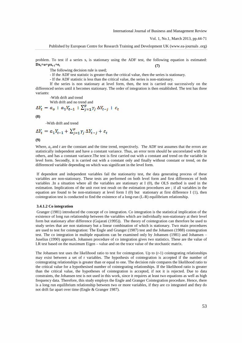
problem. To test if a series xt is stationary using the ADF test, the following equation is estimated: Dxt=α+ρxt-1+et (7) The following decision rule is used; - If the ADF test statistic is greater than the critical value, then the series is stationary. - If the ADF statistic is less than the critical value, the series is non-stationary.

If the series is non stationary at level form, then, the test is carried out successively on the differenced series until it becomes stationary. The order of integration is then established. The test has three variants:

-With drift and trend

With drift and no trend and

(8)

-With drift and trend

(9)

Where, ao and t are the constant and the time trend, respectively. The ADF test assumes that the errors are statistically independent and have a constant variance. Thus, an error term should be uncorrelated with the others, and has a constant variance.The test is first carried out with a constant and trend on the variable in level form. Secondly, it is carried out with a constant only and finally without constant or trend, on the differenced variable depending on which was significant in the level form. If dependent and independent variables fail the stationarity test, the data generating process of these variables are non-stationary. These tests are performed on both level form and first differences of both variables .In a situation where all the variables are stationary at I (0), the OLS method is used in the estimation. Implications of the unit root test result on the estimation procedures are ; if all variables in the equation are found to be non-stationary at level form I (0) but stationary at first difference I (1), then cointegration test is conducted to find the existence of a long-run (L-R) equilibrium relationship.

3.4.1.2 Co integration Granger (1981) introduced the concept of co integration. Co integration is the statistical implication of the existence of long run relationship between the variables which are individually non-stationary at their level form but stationary after difference (Gujarati (1995)). The theory of cointegration can therefore be used to study series that are non stationary but a linear combination of which is stationary. Two main procedures are used to test for cointegration: The Engle and Granger (1987) test and the Johansen (1988) cointegration test. The co integration in multiple equations can be examined only by Johansen (1981) and Johansen –Juselius (1990) approach. Johansen procedure of co integration gives two statistics. These are the value of LR test based on the maximum Eigen – value and on the trace value of the stochastic matrix. The Johansen test uses the likelihood ratio to test for cointegration. Up to (r-1) cointegrating relationships may exist between a set of r variables. The hypothesis of cointegration is accepted if the number of cointegrating relationships is greater than or equal to one. The decision rule compares the likelihood ratio to the critical value for a hypothesised number of cointegrating relationships. If the likelihood ratio is greater than the critical value, the hypotheses of cointegration is accepted, if not it is rejected. Due to data constraints, the Johansen test is not used in this work, since it requires at least two equations as well as high frequency data. Therefore, this study employs the Engle and Granger Cointegration procedure. Hence, there is a long run equilibrium relationship between two or more variables, if they are co integrated and they do not drift far apart over time (Engle & Granger 1987).


Vol. 1, No.1, March 2013, pp.44-71


54

The Engle and Granger test is a two step test which first requires that the variables be integrated of the same order. The first step consists of estimating the equation in level form, while the second step consists of testing the stationarity of the residuals, of the estimated equation. The existence of co integration is confirmed if the residuals are stationary at level form. In order to examine the short run relationships of the model, error correction model is used. Error correction term included in the model, explains the speed of adjustment towards the long run equilibrium. In addition in the present study, we have applied Granger causality test for examining the causality of the variables. In order to examine the short run relationships of the model, error correction model is used. Error correction term included in the model, explains the speed of adjustment towards the long run equilibrium. In addition in the present study, we have applied Granger causality test for examining the causality of the variables. If the variables confirm the existence of cointegration, then the conventional Vector Error Correction Model (VECM) is estimated using OLS, confirming short run dynamics and long-run equilibrium, an error correction term is constructed to estimate for coefficients. If the variables fail the cointegration test, only the short run model is estimated.

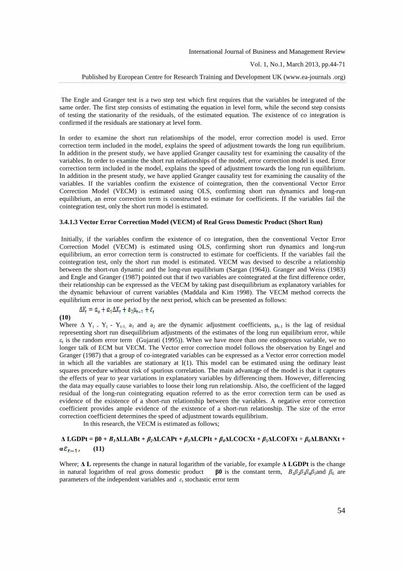
3.4.1.3 Vector Error Correction Model (VECM) of Real Gross Domestic Product (Short Run) Initially, if the variables confirm the existence of co integration, then the conventional Vector Error Correction Model (VECM) is estimated using OLS, confirming short run dynamics and long-run equilibrium, an error correction term is constructed to estimate for coefficients. If the variables fail the cointegration test, only the short run model is estimated. VECM was devised to describe a relationship between the short-run dynamic and the long-run equilibrium (Sargan (1964)). Granger and Weiss (1983) and Engle and Granger (1987) pointed out that if two variables are cointegrated at the first difference order, their relationship can be expressed as the VECM by taking past disequilibrium as explanatory variables for the dynamic behaviour of current variables (Maddala and Kim 1998). The VECM method corrects the equilibrium error in one period by the next period, which can be presented as follows:

(10)

Where ∆ Yt = Yt - Yt-1, a1 and a2 are the dynamic adjustment coefficients, µt-1 is the lag of residual representing short run disequilibrium adjustments of the estimates of the long run equilibrium error, while εt is the random error term (Gujarati (1995)). When we have more than one endogenous variable, we no longer talk of ECM but VECM. The Vector error correction model follows the observation by Engel and Granger (1987) that a group of co-integrated variables can be expressed as a Vector error correction model in which all the variables are stationary at I(1). This model can be estimated using the ordinary least squares procedure without risk of spurious correlation. The main advantage of the model is that it captures the effects of year to year variations in explanatory variables by differencing them. However, differencing the data may equally cause variables to loose their long run relationship. Also, the coefficient of the lagged residual of the long-run cointegrating equation referred to as the error correction term can be used as evidence of the existence of a short-run relationship between the variables. A negative error correction coefficient provides ample evidence of the existence of a short-run relationship. The size of the error correction coefficient determines the speed of adjustment towards equilibrium. In this research, the VECM is estimated as follows; ∆ LGDPt = β0 + Β1∆LLABt + β2∆LCAPt + β3∆LCPIt + β4∆LCOCXt + β5∆LCOFXt + β6∆LBANXt +

α (11) Where; ∆ L represents the change in natural logarithm of the variable, for example ∆ LGDPt is the change in natural logarithm of real gross domestic product β0 is the constant term, Β1β2β3β4β5and β6 are parameters of the independent variables and εt stochastic error term


Vol. 1, No.1, March 2013, pp.44-71


55

lag of the residual term representing short run disequilibrium adjustments of the estimates of the

long run equilibrium error, is the coefficient of the error correction term. Once a long-run relationship is established, then the dynamic behaviour among the relevant variables can be estimated using the VECM, where the S-R and L-R relationship are represented. However, if the Engle and Granger Cointegration test fail to justify the existence of cointegration among the variables, then only the S-R relationship in first difference form is modeled, using OLS. Note should be taken that the hypothesis tested in this study is the alternative hypothesis of the existence of a long-run relationship between the dependent and the independent variables, defined;

:

as against; :

The decision rule used is that which compares the prob (F.statistic) with the value of the level of significance. Our chosen level of significance (α) is 5%.The decision rule is that if the p-value is less than the chosen α, we accept H1, meaning the coefficients of the dependent variables are statistically significant and different from zero. But if the p-value is greater than the chosen α, we reject H1, meaning the coefficients of the dependent variables are statistically insignificant and equal to zero.

4. PRESENTATION AND ANALYSES OF RESULTS

Before going to provide a comprehensive econometric analysis, we give the brief interpretation of statistical analysis. Table 1 report the descriptive statistics and interprets that the average GDP at market prices is 10200000000fcfa with a 4.80E+09 standard deviation. The average fixed capital formation is 3160000000 fcfa. The mean value of labor force is 4825883 people with standard deviation of 1583119 .The average consumer price index is 64.00006 with a standard deviation of 31.37284. On the average cocoa export is 117685.3 tons, with a standard deviation of 123524. From 1975 to 1982, cocoa has been exported in Cameroon below its average export. By 1983, cocoa export has an increment of 676880 tons from it mean export. After this period cocoa exported from Cameroon stood low from its mean value. This could be attributed to the economic crisis which affected all the sectors of the economy. After this period its export went above its average. The average coffee export is101546.3 tons, with a standard deviation of 112462.8.In Cameroon, coffee export stood below its average from 1975 to 1983, where it witness an increase two years later. By 1989 to 1992 export fell below averages with a continuous increment where it reaches its peak in 1998. After this year coffee has been exported around its mean export. On the average banana export is 140410.9, with a standard deviation of 90333.54.From 1975 to 1993 bananas has been exported below its mean value. But after this period on ward banana export witness a dramatic increase above its mean value. This could be attributed to many reform programs that have been put in place by the government. Skew ness is a measure of departure from symmetry. The variable LNCPI, included in our analysis is negatively skewed or is leftward skewed, while the variables (LNGDP, LNCOCX, LNCAP, LNLAB and LNCOFX) are positively skewed or are rightward skewed. Kurtosis measures the peaked ness or flatness of the data relative to the normal distribution. The coefficient of Kurtosis of the variables indicate that coffee export and banana export are Plato – kurtic or flat while all other variables in our study have peaked ness or lapto kurtic. Skewness and Kurtosis jointly determine


Vol. 1, No.1, March 2013, pp.44-71


56

whether a random variable follows a normal distribution. Table 1: Descriptive statistics

Source: calculations by Authors using Eviews 7

GDP CAP LAB CPI COCX COFX BANX

Mean 1.02E+10 3.16E+0

9

4825883. 64.00006 117685.3 101546.3 140410.9

Median 9.84E+09 1.88E+0

9

4655033. 54.78525 89930.00 88863.00 116000.0

Maximum 2.37E+10 2.93E+1

0

7727247. 115.1500 794565.0 723125.0 313723.0

Minimum 2.26E+09 1.54E+0

8

2355532. 15.17833 16977.00 32925.00 20231.00

Std. Dev. 4.80E+09 5.14E+0

9

1583119. 31.37284 123524.0 112462.8 90333.54

Skewness 0.684724 4.28335

0

0.200579 -0.006469 4.881303 5.006551 0.428397

Kurtosis 3.734018 21.2121

6

1.929881 1.658360 27.33135 28.27574 1.768299

Jarque-Bera 3.520663 590.728

7

1.904702 2.625242 1002.346 1077.891 3.282978

Probability 0.171988 0.00000

0

0.385833 0.269114 0.000000 0.000000 0.193691

Sum 3.59E+11 1.10E+1

1

1.69E+08 2240.002 4118987. 3554120. 4914380.

Sum Sq. Dev. 7.83E+20 8.99E+2

0

8.52E+13 33464.66 5.19E+11 4.30E+11 2.77E+11

Observations 35 35 35 35 35 35 35


Vol. 1, No.1, March 2013, pp.44-71


57

The main objective of the study is to explore the contribution of selected agricultural exports crops on economic growth, both in the long run and in the short run. Engle and Granger tests for cointegration is used. Once the problem of spurious regression is detected, the next step in the time series econometrics is to examine the stationarity of the variables for determining the order of integration.

4.1 Presentation of Engle and Granger Method of Cointegration Analysis

Here the procedure is going to be carried out in two steps after determining the order of integration of the variables through the unit root test. Step1, which consist of the long run relationship that we wish to verify its existence is first of all estimated using ordinary least squares with all the variables in level. Step 2 consists of extracting the error resulting from this regression and the unit root test conducted on it. The stationarity of the error at level form depicts a long run relationship between the variables. If not, the relationship does not exist. The absence of a long run relationship between the variables, imply that we have to run an ordinary least squares regression with I(0) variables in level form and I(1) in first difference, I(2) in second difference and so on, so as to get consistent results. In our case, we are going to present the unit root results first, closely followed by the estimation of the long run relationship. We shall then extract the error term (denoted ECT) on which we carry out a unit root test at level form I(0) in order to confirm the existence of cointegration. If cointegration exists, then we estimate the error correction model. For the error correction model, we difference all the variables and include the error correction term lagged by two period ECT (-1) to capture the effects of year to year variations. We are expecting that the coefficient of ECT (-1) to be significantly negative and less than one for the error correction mechanism to exist. The essence of using error correction model in the case of cointegration allows getting more reliable estimates than those we could have had if we had use the long term relationship.

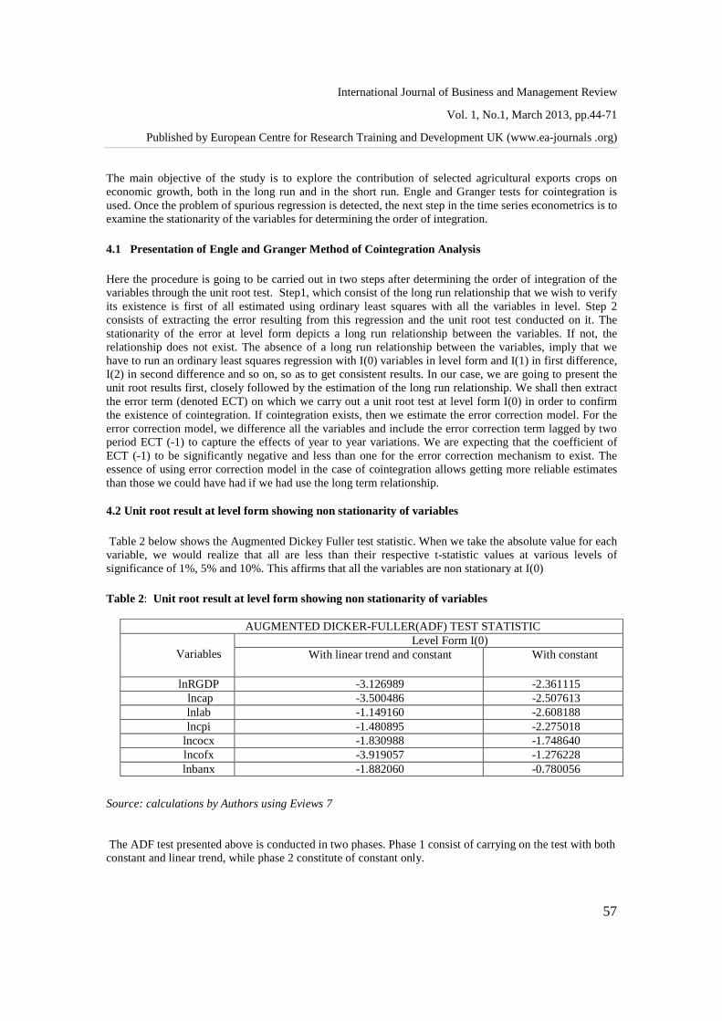
4.2 Unit root result at level form showing non stationarity of variables Table 2 below shows the Augmented Dickey Fuller test statistic. When we take the absolute value for each variable, we would realize that all are less than their respective t-statistic values at various levels of significance of 1%, 5% and 10%. This affirms that all the variables are non stationary at I(0)

Table 2: Unit root result at level form showing non stationarity of variables

AUGMENTED DICKER-FULLER(ADF) TEST STATISTIC

Variables Level Form I(0)

With linear trend and constant With constant

lnRGDP -3.126989 -2.361115 lncap -3.500486 -2.507613 lnlab -1.149160 -2.608188 lncpi -1.480895 -2.275018

lncocx -1.830988 -1.748640 lncofx -3.919057 -1.276228 lnbanx -1.882060 -0.780056


The ADF test presented above is conducted in two phases. Phase 1 consist of carrying on the test with both constant and linear trend, while phase 2 constitute of constant only.


Vol. 1, No.1, March 2013, pp.44-71


58

4.3 Presentation of stationarity of variables using unit root results at first difference

The figures on table 2 equally show the Augmented Dickey Fuller test statistic, which in absolute terms for each variable, are all greater than their respective t-statistic values. This confirms that all the variables are stationary at I (1).

Table 3: Unit root result at first difference showing stationarity of variables

AUGMENTED DICKER-FULLER TEST

Variables First Difference I(1)

With Trend and Constant With constant Decision

lnRGDP -6.011046*** -6.121348*** I(1) lncap -6.677479*** -6.721650*** I(1) lnlab -6.50541*** -3.861960*** I(1) lncpi -5.227059*** -4.319720*** I(1) lncocx -5.565587*** -5.599466*** I(1) lncofx -5.536966*** -5.595110*** I(1) lnbanx -4.165169*** -4.224071** I(1)

Note: *** indicates significance at 1%, ** indicates significance at 5% Source: calculations by Authors using Eviews 7 The ADF test results in table 4 shows that all the variables are integrated of order one. The variables lnRGDP, lncap, lnlab, lncpi, lncocx, lncofx and lnbanx are all stationary at first difference. Our model in equation (6) is going to enable us to estimate the long run relationship. Following the Engle and Granger procedure, we have to run the OLS of our model, then extract the error term of this relationship and test whether it is stationary at level form. That is to say I (0). If it is the case, then the long run cointegration relationship exists. Table 4 displays the unit root results of the error correction term: Table 4: Unit root test of Error Correction Term Null Hypothesis: ECT has a unit root Exogenous: Constant Lag Length: 1 (Automatic - based on SIC, maxlag=8)

t-Statistic Prob.* Augmented Dickey-Fuller test statistic -4.491151 0.0012

Test critical values: 1% level -3.661661 5% level -2.960411 10% level -2.619160


The results in table 4 shows that the ADF test statistic in absolute term is greater than all the test critical values thus indicating that the error (ECT) from the regression using OLS is stationary at 1% level of significance and at level form I (0). As such, we reject the Null Hypothesis. This confirms the existence of cointegration. The long run results can therefore be interpreted after verifying the appropriateness of the model.


Vol. 1, No.1, March 2013, pp.44-71


59

4.4 Model Appropriateness

Autocorrelation Test Autocorrelation refers to the existence of a relationship between error terms across observations of a time series. Error covariances are therefore different from zero. This constitutes a violation to one of the assumptions of the classical linear model. Autocorrelation is manifested by OLS estimators which are not BLU (Best linear unbiased). In our study, auto correlation is going to be tested using the Breusch-Godfrey serial correlation LM test. The Durbin-Watson test is not used because it is biased. The decision rule is to accept H0 if the probabilities of the F-statistic and the observed R2 of the intermediary equation are greater than 0.05, which depict the absence of auto correlation. On the other hand, H1 is not rejected if the probabilities of the F-statistic and the observed R2 of the intermediary equation are lesser than 0.05. The test results are shown on table 5. Table 5: Autocorrelation test results

Breusch-Godfrey Serial Correlation LM Test:

F-statistic 1.121460 Prob. F(2,23) 0.3430

Obs*R-squared 2.932164 Prob. Chi-Square(2) 0.2308

Source: calculation by authors using Eviews 7

From the test results presented on table 5, the probabilities of both the F-statistic (0.3430) and the R-squared (0.2308) are greater than 0.05. Therefore, Ho is not rejected, meaning autocorrelation is absent.

4.5 Heteroscedasticity Test

In order to ensure that the residuals are randomly dispersed throughout the range of the dependent variable, we are going to use the heteroscedasticity test. The variance of the error should therefore be constant for all values of the dependent variable. In the presence of heteroscedasticity, the distributions of the OLS parameters are no longer normal. Heteroscedasticity is tested in this study using the Breusch-Pagan-Godfrey test.

The decision rule is to reject the null hypothesis if the probability of the F-statistic and observed 2R are less than 0.05, meaning heteroscedasticity is present. On the other hand, if the probability of the F-statistic

and observed 2R are greater than 0.05, we do not reject the null hypothesis, implying that there is no heteroscedasticity. As such, errors are homoscedastic. The test results are shown on table 6:

Table 6: Heteroscedasticity Test

Heteroskedasticity Test: Breusch-Pagan-Godfrey

F-statistic 1.140708 Prob. F(6,26) 0.3672

Obs*R-squared 6.876702 Prob. Chi-Square(6) 0.3324

Scaled explained SS 9.324447 Prob. Chi-Square(6) 0.1561


Vol. 1, No.1, March 2013, pp.44-71


60


From the test results presented on table 6, both the probabilities of F-statistic (0.3672) and the R-squared (0.3324) are greater than 0.05 indicating the absence of heteroscedasticity. Therefore, the errors are homoscedastic. Therefore the long run results succeed all tests and thus useful for analyses and forecasting.

4.6 Results of Long run relationship

Table 7 displays the results of the long run relationship between agricultural export variables and economic growth using equation (7). Table 7: Long run relationship between agricultural export and economic growth

Dependent variable: lnRGDP; Method: Least Squares

Variable Coefficient C 18.08662***

(6.524075) lnCAP 0.037132*** (0.085298)

lnLAB 0.018639*** (0.159796)

lnCPI 0.107900*** (0.780976) lnCOCX -0.437935*

(0.267716) lnCOFX 0.352921*** (0.348447) lnBANX 0.453739*** (0.161193) Adjusted R-squared 0.698150 F-statistic 8.260371 Prob(F-statistic) 0.000032 Durbin-Watson stat 1.740409

Included observations 33

Note: Standard errors are in parentheses; * indicates significance at 10%,

** indicates significance at 5%, and *** indicates significance at 1%.


Globally, we can observe that all the results from the test statistics of the model are good. As a matter of fact, the adjusted R square is high (about 69.8%). This means that the independent variables explain the dependent variable for about 69.8 percent. The overall significance of the model is good at 1% through the prob (Fisher- statistic). It is important to mention here that the decision rule used is that which compares the prob (F.statistic) with the value of the chosen level of significance (5%). The p-value (0.000032) from table 8 is less than 0.05. As such, we accept the alternative hypothesis, implying that the parameters are generally significant even at 1%.


Vol. 1, No.1, March 2013, pp.44-71


61

In addition, almost all the coefficients are individually significant at 1% level of significance, except lnCOCX which is only significant at 10%. We can also observe that there is a positive relationship between the dependent variable (lnRGDP) and four independent variables (lnCOFX, lnBANX), lnCAP, lnLAB and lnCPI). This means that if one of these independent variables increases, the dependent variable will also increase and vice versa. These results are in accordance with what we expected but lnCOCX contradicts our expectations.

4.7 Discussion of the Effects of explanatory Variables on the Real GDP

4.7.1 Discussion of the effect of agricultural export Variables on Economic growth from our results Here we would made mention of the three agricultural export variables used in our work to see if they answer our specific alternative hypotheses. These variables are cocoa export, coffee export and banana export.

1) Effect of Cocoa Export on Economic Growth Findings from our results reveal that Cocoa export has a negative and insignificant effect on economic growth in Cameroon, which refute our first specific alternative hypothesis. This result is contradioctory with most of what is found in literature. Shashi K.and Marcel V. (2010) looks at cocoa in Ghana: shaping the success of the economy. He noticed a positive effect between the cocoa sector and economic growth in Ghana, which contradicts our result. This negative correlation is as a result of a general decline in production, productivity, quality of cocoa bean and price, which resulted in the abandonment of several plantations experienced during the first phase of liberalization. In Cameroon, cocoa is grown in either intensive or extensive production systems, or in a combination of the two by family units. Cocoa production is labour intensive and requires a substantial portion of available manpower in the production areas. The inadequate labour has led to the employment of children in most of the farms which result to low output. We could also cite the problem of cocoa beans being exported raw with no value added through processing. These problems reduces the exchange value from the sale of this cash crop

2) Effect of Coffee Export on Economic Growth The results of study reveal that coffee export has a positive and significant effect on economic growth in Cameroon, which affirms the second specific alternative hypothesis. According to Paulo P. (2000) who look at the role of coffee in social and economic development of Latin America; points out the evidence that during the second half of the nineteenth century up to the world economic crisis of the 1930s, the coffee sector played an important role in many countries such as Brazil, Colombia, Costa Rica, and a bit later and to a lesser degree in other countries in South and Central America. For example, around 1995, coffee represented around seventy percent of Brazil’s total exports and around eighty percent of Colombia’s total exports. Coffee production also stimulated the insertion of Latin American economies in the world trade. In this period, given its high level of dependence on external markets, the price of coffee was the principal factor in guaranteeing equilibrium in the balance of payments and, as a consequence, guaranteeing macroeconomic stability and economic growth. Income generated by coffee production and exports created domestic demand in the industrial sector in many countries, allowing for the diversification of their economies. Similarly, Roberto Junguito and Diego Pizano (2001) remind us that the economic relevance of coffee was not limited to its impact on growth via increased exports. They suggest that coffee has had a clear link with the development of other sectors and with the overall development process of Colombia. Among other impacts they stress the links between coffee production with employment and the social situation given the


Vol. 1, No.1, March 2013, pp.44-71


62

activity’s high demand for labour, its relation with public finances, its impact on industrial, regional, and institutional development and its role in national politics.

3) Effect of Banana Export on Economic Growth

Our finding reveals that banana export has a positive and significant relationship on economic growth in Cameroon, which answers our third specific alternative hypothesis. This result is equally in line with most of what is found in literature. FAO (2001) provided evidence according to which banana exports play a small but growing role in Ghana's export trade. Bananas constitute about 13 percent of horticultural exports but only about half of one percent of total exports by value. While bananas have lesser importance as a basic food item, they have become an important export commodity. Bananas provide jobs and significant incomes for hundreds of plantation workers.. Bananas are also increasingly important to export diversification, potentially enabling Ghana to earn more foreign currencies and an increase in her gross domestic product. Still in line with the same research done by FAO; Ecuador (the largest banana exporting country on the international market) earned more than US$900 million from banana export .It is calculated that in 2000 there were approximately 1.1 million people benefiting directly or indirectly from the export banana industry in Ecuador, out of a population of some 12.5 million. The export from banana has gone along way to contribute to Ecuador’s growth in the agricultural and manufacturing sector and to the economy as a whole.

4.7.2 Control Variables This work made use of three control variables such as gross domestic fixed capital, labour force and consumer price index. The first two factors are initial inputs in the production function that we want to see their effects equally on growth. The last variable is the proxy for inflation which we also want to see its effect on economic growth. The essence of using these variables is to improve on the validity and reliability of our results. i)Discussion of the effect of gross domestic fixed capital on Real GDP from Results The results from our finding show that gross domestic fixed capital has a positive and significant effect on economic growth in Cameroon. This is equally in line with the work of Bakare (2011), using the H-D model, proved that the growth rate of national income in Nigeria is positively related to saving ratio and capital formation. Moreover, Njong (2008) reveals that FDI (Foreign Direct Investment) inflows have had a positive impact on Cameroon’s export performance. Since Export earnings constitute an important proportion of our real GDP, it will lead to an increase in our real GDP. Khan and Kumar (1997), confirmed that gross domestic fixed capital (public and private investment) have significant impacts on economic growth in developing countries. ii) Discussion of the effect of labour force on Real GDP from Results From our findings there is a positive and significant relationship between the dependent variable and labour force expansion in Cameroon. This means that labour force expansion and economic growth in this study move in the same directions. The result of the labor force (LLAB) indicates that economic growth increases by about 15.98 percent due to an addition of one percent in labor force. This is supported by other authors who have previously looked at the correlation between labour force expansion and economic growth. Equally Ajab Amin (2002) in his work confirmed that one of the sources of economic growth in Cameroon is from an active labour force. iii) Discussion of the effect of inflation (lnCPI) on Real GDP from Result The results from our findings show a positive relationship between inflation and economic growth in Cameroon. This is seen as on table 8 which shows that a one percent change in inflation will lead to a 10.79 percent change in economic growth. This is inline with the work of Eishareif, Elgilani Eltahir (2007) who worked on “Term Structure, Inflation, and Economic Growth in Selected East Asian Countries”, saw a


Vol. 1, No.1, March 2013, pp.44-71


63

positive relationship between inflation and economic growth. Equally, Muhammad Zahir Faridi (2009) looked at the contribution of agricultural export to economic growth in Pakistan saw a negative and insignificant relationship between inflation and economic growth . Our result contradicts what we expected.

4.8 Results of the Vector Error Correction Model

However, we can now estimate the vector error correction model from equation (12) since we have successfully carried out almost all the necessary test of model appropriateness. Table 8 displays the results of our Vector Error Correction Model.

Table 8: Results of Vector Error Correction Model

Dependent variable: D (lnRGDP); Method: Least Squares

Variable Coefficient C 0.052578

(0.155361) D(LNCAP) 0.029920

(0.080351) D(lnLAB) 6.711105

(0.147335)

D(lnCPI) 0.250626 (1.777392)

D(lnCOCX) -0.612864* (0.309677)

D(lnCOFX) 0.539179* (0.387885)

D(lnBANX) 0.459347* (0.227130)

ECT(-1) -0.224435 * (0.790869)

Adjusted R-squared 0.222080 F-statistic 2.070546 Prob(F-statistic) 0.084480 Durbin-Watson stat 1.864388 Observations (adjusted) 31


In table 8, we can deduce that both dependent and independent variables are stationary at first difference. This is because the coefficient of the error correction term is negative, less than unity (-0.2244) and highly significant at 1%. Also following the results obtain as on table 7, it shows that a priori the expected signs of all the parameter estimated were not met. We would equally carried out the autocorrelation and heteroscedasticity test in order to confirm appropriateness of our short run VECM .The same tests which were used in the long run model, are equally applied in the VECM. We are going to start with the autocorrelation test, using the Breusch-Godfrey serial correlation LM test. The result of this test is shown on table 9 below. Table 9: Breusch-Godfrey serial correlation LM test of the VECM.

F-statistic 1.121460 Probability 0.3430


Vol. 1, No.1, March 2013, pp.44-71


64


From table 9, the probabilities of both F-statistic and R-squared are greater than 0.05, confirming the absence of autocorrelation. The test for heteroscedasticity was also conducted using the Breusch-Pagan-Godfrey Test. The following results were obtained on table 10. Table 10: Heteroskedasticity Test: Breusch-Pagan-Godfrey

Source: calculations by Authors using Eviews 7 From table 10, we can notice the absence of heteroscedasticity since the probabilities of both F-statistic and R-squared are greater than 0.05. Thus, the errors from the VECM are homoscedastic. The VECM is void of autocorrelation and heteroscedasticty and can now be interpreted. Other observations in our model are as follows; The Durbin Watson d statistics of 1.864 is greater than the adjusted R-squared of 0.222, meaning that our VECM does not suffer from a spurious regression. The F-statistic is 20.705 which is quite high and most interestingly is highly significant at 1%. The results also reveal that our exogenous variables did not all have the expected signs. For our variables of interest, coffee export and banana export have a positive effect on economic growth while cocoa export has a negative effect on economic growth, which contradicts what we expected. The reason for this has earlier been explained. Our control variables; gross domestic fixed capital and labour force expansion has positive effect on growth which is inline with what we expected. Inflation also witnesses a positive correlation with economic growth which contradicts our expected results. The coefficient of the ECT is, -0.224435 is highly significant at 1% percent and has the appropriate negative sign. Thus, it will rightly act to correct any deviations from the long-run equilibrium up to the tune of 22.44%, which is fair. This fair significant value of the VECM explains the existence of long-run equilibrium relationship between agricultural export and economic growth in Cameroon. This established long-run equilibrium relationship in our result reveals that our findings can be used for forecasting and policy recommendation (s) .We would proceed with the long causality test and the causality test on VECM of important variables. Granger (1969) causality test has been performed in order to examine the linear causation between the concerned variables. Granger causality is useful in determining the direction of the relationships. In the view of the Granger, the presence of co-integration vector shows that granger causality must exist in at least one direction.

R-squared 2.932164 Probability 0.2308

F-statistic 0.797231 Prob. F(7,22) 0.5979 Obs*R-squared 6.070148 Prob. Chi-Square(7) 0.5316 Scaled explained SS 9.717758 Prob. Chi-Square(7) 0.2051


Vol. 1, No.1, March 2013, pp.44-71


65

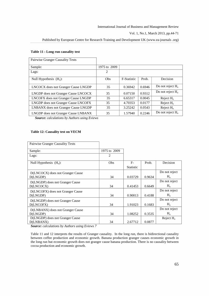
Table 11 : Long run causality test Pairwise Granger Causality Tests

Sample: 1975 to 2009 Lags: 2

Null Hypothesis (Ho): Obs F-Statistic Prob. Decision

LNCOCX does not Granger Cause LNGDP 35 0.36942 0.6946 Do not reject Ho

LNGDP does not Granger Cause LNCOCX 35 0.07150 0.9312 Do not reject Ho

LNCOFX does not Granger Cause LNGDP 35 6.65317 0.0045 Reject Ho LNGDP does not Granger Cause LNCOFX 35 4.70353 0.0177 Reject Ho LNBANX does not Granger Cause LNGDP 35 3.25242 0.0543 Reject Ho

LNGDP does not Granger Cause LNBANX 35 1.57940 0.2246 Do not reject Ho

Source: calculations by Authors using Eviews

Table 12: Causality test on VECM

Pairwise Granger Causality Tests

Sample: 1975 to 2009 Lags: 2

Null Hypothesis (Ho): Obs F-Statistic

Prob. Decision

D(LNCOCX) does not Granger Cause D(LNGDP) 34 0.03729 0.9634

Do not reject Ho

D(LNGDP) does not Granger Cause D(LNCOCX) 34 0.41453 0.6649

Do not reject Ho

D(LNCOFX) does not Granger Cause D(LNGDP) 34 0.90013 0.4188

Do not reject Ho

D(LNGDP) does not Granger Cause D(LNCOFX) 34 1.91023 0.1683

Do not reject Ho

D(LNBANX) does not Granger Cause D(LNGDP) 34 1.08252 0.3535

Do not reject Ho

D(LNGDP) does not Granger Cause D(LNBANX) 34 2.67712 0.0877

Reject Ho

Source: calculations by Authors using Eviews 7 Table 11 and 12 interprets the results of Granger causality. In the long run, there is bidirectional causality between coffee production and economic growth. Banana production granger causes economic growth in the long run but economic growth does not granger cause banana production. There is no causality between cocoa production and economic growth.


Vol. 1, No.1, March 2013, pp.44-71


66

Granger causality test on vector error correction model show the direction of the relationship amongst our variables of interest. Among all the variables of interest, causality runs only from real GDP to banana production in the short run. There is no causality between the real GDP and the other selected agricultural products in the short run.

5. Policy RECOMMENDATIONS, CONCLUSION AND SUGGESTION FOR FURTHER RESEARCH

5.1 Policy Recommendations

Following the results of our study, we can recommend long run growth policies to be used by the government holding some all others constant. Findings regarding the contribution of agricultural export to economic growth and the relatively high value of the elasticity coefficients imply that the government of Cameroon can use the agricultural export development policy to spur economic growth at the national level. Looking at the long run relationship between both the exogenous/control variable(s) and economic growth we can specifically recommend the following policies: 1) The results from our findings reveal a negative insignificant correlation between cocoa exports with real GDP in Cameroon. This is mainly due to the fact that production of cocoa is carried out by individual families with small income and thus produces on a small scale. Most often the producers lack the material and financial means to maintain the quality of the cocoa bean from when it is produce to when it is taking to the market. Thus the small output of low quality affects the price offered at the world market since the value of cocoa bean depends on the productivity and the quality. As a policy, the government should encourage farmers to form cooperatives so that they could be open to loan schemes which will go a long way to increase productivity. Also the government should finance research activities on improving on the quality of cocoa produced and sold oversea. There should be serious selection of cocoa bean at the port in order to avoid the mixing of good cocoa beans with the bad ones in shipments for export 2) Equally our results depict a positive and significant correlation between coffee export and real GDP in Cameroon. The government of Cameroon should put in place policies to stimulate the coffee sector through the encouragement of farmers to form cooperative, financial aid given to farmers, intensive research on improvement of quality coffee green being carried out, organization of seminars comprising of all parties (the coffee producing board, farmers, exporters, manufacturing companies who uses coffee as raw material and other stake holder in the sector). Also coffee production should equally be carried out on a large scale by companies which will help to maintain quality and thus an increment in its value. 3) Also banana export equally has a positive and significant long effect on real GDP following the result of our findings. This could be attributed to large scale production with quality maintenance from CDC and ASSOBACAM. The government should increase the participation of private companies in this sector so as to increase total output. More research on quality maintenance, tropical diseases affecting banana crop should be carried out or finance so as to increase the yields from the sale of banana. 4) In the light of our control variables inflation showed a positive and significant relationship with economic growth in Cameroon. The positive effect could have been as a result of the series of price fluctuation faced by these goods. The results of capital and labour (the core factors of production of growth) reveal a positive effect on real GDP. The study reports the more share of capital in economic growth as compared with labour’s share in growth. This is because Cameroon is a growing economy wherein physical l capital is growing faster than human capital. There should be an increase in investment of both public and private in Cameroon. While the government should redress the problems disturbing the labour force from constantly and consistently growing.


Vol. 1, No.1, March 2013, pp.44-71


67

Labour force expansion equally shows a positive and significant effect on economic growth in Cameroon. The government should put in place measures to fight against brain drain. There should be a synergy between universities and promoters of company that is the university system should be restructured to offer courses which tie-up with jobs in the domestic labour market. It should equally stimulate the private sector to create jobs there by reducing the level of unemployment. The government should put in place measures of growth in human stock of capital through expansion of educational system, skill and training facilities and provision of better health facilities even in rural or backward areas of the country. Besides these, there should be an increase in investment in education and health in private sector with the co operation of industrially advanced countries. It should encourage auto-employment amongst her nationals. The putting in place of these measures would reduce the rate of unemployment in the country and thus have a trigger effect on economic growth in Cameroon.

5.2 Conclusion

The raison of our study was to investigate if agricultural export has a positive and significant effect on economic growth in Cameroon, for period 1976 to 2009. In order to attain the objective of our study, we used the standard theoretical neoclassical growth model, based on a generalized Cobb Douglas production framework with some extensions. As concerns economic analysis, the ADF test was used to test for stationarity, Engle and Granger cointegration analysis was used to determine long and short run relationships. The Arch test and the Breusch-Godfrey Serial Correlation LM Test, was used to test for appropriateness of our estimations in order to avoid any spurious regression. The results indicate that agricultural export variables have mixed effects on domestic growth. A positive and significant association is found between coffee export and economic growth. Equally a positive significant effect is found between banana export and economic growth in Cameroon. The reverse was true with cocoa export which shows a negative and insignificant effect on economic growth in Cameroon. As concerns our control variables, Capital was found to have a positive significant effect on economic growth, which confirms that agricultural capital has a positive significant effect on economic growth. We also found out that in the context of Cameroon, labour force expansion has a positive and significant impact on economic growth. It is equally revealed that inflation has a positive and significant effect on real GDP in Cameroon. However, for the purpose of contribution to knowledge, it is necessary for other developing countries like Cameroon faced with a budget constraint to undertaken specific policy recommendations. Most of what is found in literature around this area emphasis on the need to develop the agricultural sector as a whole. Cameroon being a third world country needs to invest in specific agricultural products following the big push theory like those in this study, in order to achieve its dream of becoming an emerging economy by the year 2035.

5.3 Limitations and Scope for further Research

Our study has certain limitations and could not exhaust all aspects of agricultural export, in relation to the national and the regional level in Cameroon. For example, looking at the contribution of other agricultural exports other than the ones we have use to economic growth in Cameroon are not discussed. Furthermore, issues on the effect of non agricultural export to economic growth are not discussed. Since it is clear from this study that agricultural export contributes to economic growth, the direct contribution of primary commodity export on economic growth needs to be assessed in terms of scope and degree of impact. However, for policy making, it is important to find out the effectiveness and impact of value chain finance of agricultural products on economic growth, why not specifically in Cameroon. Not with standing other research work could dwell on the economic impact of climate change on agricultural export in any choice of country.


Vol. 1, No.1, March 2013, pp.44-71


68

REFERENCES Abdul Ghafar Ismail and D. Agus Harjito, (2000) “Export and economic growth: The Causality Test for

ASEAN Countries” pp. 1- 5 and pp. 40 - 55.

Ahmad, J. and Kwan, A.C.C. (1991), “Causality between exports and economic growth”. Economic Letters, 37, pp. 243 - 248.

Alisi Wenonalita & Kautoke-Holani (2008), “Agricultural Export Growth and Economic Development for Tonga: The Quest for Efficiency”.

Aloysius A. A. (March 2002), “An examination of the sources of economic growth in Cameroon”; pp. 1-20 Published by: The African economic research consortium (AERC) Nairobi Kenya

Amin, Aloysius Ajab (1996), “The Effects of Exchange Rate Policy on Cameroon’s Agricultural Competitiveness”. AERC Research Paper No. 42. Nairobi.

Amin, Aloysius Ajab (1998), “Cameroon’s Fiscal Policy and Economic Growth.” AERC Research Paper No. 85. Nairobi.

André C. Jordaan & Joel Hinaunye Eita, (2007) “Testing the Export-Led Growth Hypothesis for Botswana: A Causality Analysis”, pp. 2 - 9.

Aurangzeb (2006), “Exports, productivity and economic growth in Pakistan: a time series Analysis”. The Lahore Journal of Economics, 11(1), 1-18.

Bahamani-Oskooee, M., Mohtadi, H. and Shabsigh G. (1991), “Exports, growth and Causality”. Journal of Development Economics, No.36, pp. 405 - 415.

Bahmani-Oskooee, M. and Alse, J. (1993), “Export growth and economic growth: an application of cointegration and error-correction modeling”. Journal of Developing Areas, No.27(4), 535 - 542.

Balassa, B. (1978), “Exports and growth: further evidence”. Journal of Development Economics, 5, 181–189. Balassa, B. (1985), “Exports, policy choices, and economic growth in developing countries after the 1973 oil

shock”. Journal of Development Economics, No.18, pp. 23 - 35. Chenery, H.B. and Strout, A. (1966), “Foreign assistance and economic development”. American Economic

Review, No. 56, pp. 680 - 733. Chow, P.C.Y. (1987), “Causality between export growth and industrial development”. Journal of Development

Economics, No. 26, pp. 55 - 63. Daniel Gbetnkon and Sunday A. Khan, (2002), “Determinants of agricultural export in Cameroon” pp1 - 45. Darrat, A. (1987), “Are Exports an Engine of Growth? Another Look at the Evidence”. Applied Economics,

No.19, pp. 277 - 83. Dawson, P.J. (2005), “Agricultural exports and economic growth in less developed Countries”. Agricultural

Economics, No.33, pp. 145 - 152. Dickey, D. and Fuller W. (1981), “Likelihood ratio statistics for autoregressive time series with a unit root”.

Econometrica, No.49, pp.1057 - 1072. Dorado, S. (1993), “Exports and Growth: A reconsideration of causality”. Journal of Developing Areas, No.27,

pp. 227 - 244. Dutt, S.D. and Ghosh, D. (1994), “An empirical investigation of the export growth economic growth

relationship”. Applied Economic Letters, No.1, pp. 44 - 48. Ekanayake, E.M. (1999), “Exports and economic growth in Asian developing countries: Co-integration and

error correction models”. Journal of Economic Development, 24(2), pp. 43 - 56 Ekpo A, Egwaikhide F (1994), “Exports and Economic growth in Nigeria: A Reconsideration of the evidence”,

Journal of Economic Management, No. 1 pp. 100 – 115 Feder, G. (1983), “On exports and economic growth”. Journal of Development Economics No., 12, pp. 59 -73. Fosu, A. K. (1990), “Export Composition and the Impact of Export on Economic Growth of Developing

Economies”. Economics Letters, No. 34, pp. 67 -71. Ghartey, E.E. (1993), “Causal Relationship between Exports and Economic Growth: Some Empirical Evidence

in Taiwan, Japan and the US”. Applied Economics, No. 25, pp. 1145 -52. Ghatak, S., Milner, C. and Utkulu, U. (1997). “Exports, export composition and growth: Cointegration and

causality evidence for Malaysia”. Applied Economics, 29(2), pp. 213 - 223. Gorden, D.V. (1995), “Optimal Lag Length in Estimating Dickey-Fuller Statistics: An Empirical Note”.

Applied Economics Letter, Vol. 2, pp. 188 - 90.


Vol. 1, No.1, March 2013, pp.44-71


69

Granger, C.W.J. (1969), “Investigating causal relations by econometric and cross-spectral Method”. Econometrica, 37(3), pp. 424 - 438.

Granger, C.W.J. (1988), “Some recent developments in a concept of causality”. Journal of Econometrics, No.39, pp.199 - 211.

Granger, C.W.J., Newbold, P. (1974), “Spurious regression in econometrics”. Journal of Econometrics, No. 2, pp. 111 - 120.

Heller, P.S. and Porter, R.C. (1978), “Exports and growth: an empirical reinvestigation”. Journal of Development Economics, No. 5, 191 - 193.

Holman, J.A. and Graves, P.E. (1995), “Korean exports economic growth”: an econometric reassessment. Journal of Economic Development, No.20, 45 - 56.

IMF (1999), “International Financial Statistics Yearbook”. Islam, M.N. (1988), “Export expansion and economic growth: testing for cointegration and causality”. Applied

Economics, No.30, pp. 415 - 425. Jin, J.C. and Yu, E.S.U. (1995), “The causal relationship between exports and income”. Journal of Economic

Development, No. 20(1), 131 - 140. Johansen, S. (1988), “Statistical analysis of cointegration vectors”. Journal of Economic Dynamics and

Control, No.12, 231 - 254. Johansen, S. and Juselius, K. (1990). Maximum likelihood estimation and inference on Cointegration with

application to the demand for money. Oxford Bulletin of Economic and Statistics, No.52, pp. 169 - 210. John Joseph Puthenkalam (1998, 2000&2009), “Integrating Freedom, Democracy and Human Rights into

Theories of Economic Growth”. Johnston, B.F. and Mellor, J.W. (1961), “The role of agriculture in economic Development”. American

Economic Review, 51, pp. 566 - 593. Jonathan Coulter and Pierre E. Abena (2010), “Study of the value chain finance for coffee and cocoa in

Cameroon”. pp. 1 - 50. Joshi, Rakesh Mohan, (2005), “International Marketing”, Oxford University Press, New Delhi and New York,

pp. 10 - 15. Jung, W.S. and Marshall, P.J. (1985), “Exports, growth and causality in developing Countries”. Journal of

Development Economics, No.18, pp. 1-12. Justin N. Okolle, Gabriel H. F., Franklin M. Lombi, Patrick S. Lang & Pierre M. Loubona (2009) “Banana

Entomological Research in Cameroon: How far and what Next?” The African Journal of plant science and Biotechnology.

Kavoussi, R.M. (1984), “Exports Expansion and Economic Growth: Further Empirical Evidence”. Journal of Development Economics, No. 14, pp. 241 - 50.

Khan, A.H. and Saqib, N. (1993), “Exports and economic growth: The Pakistan Experience”. International Economic Journal, No.7 (3), pp. 55 - 64.

Kormendi, R.C. and Mequire, P.G. (1985), “Macroeconomic determinants of growth: cross-country evidence”. Journal of Monetary Economics, No.16 (2), pp. 141-163.

Kugler, P. (1991), “Growth, exports and cointegration: An empirical investigation”. Weltwirtschaftliches Archive, No. 127(2), pp. 73 - 81.

Kunst, R.M. and Marin, D. (1989), “On exports and productivity: A causal analysis”. Review of Economics and Statistics, No.71, pp. 699 - 703.

Kwa and Bassoume (2007), “Exploring the linkages between agricultural exports and sustainable development”. Ecofair trade dialogue [Discussion Paper] No. 2, pp. 1 - 38.

Levin, A. and Raut, L.K. (1997), “Complementarities between exports and human capital in economic growth: evidence from the semi-industrialized countries”. Economic Development and Cultural Change, No.46, pp.155 - 174.

Michael Ndoping, (2011), “A speech at Angossas, 300 kilometers (186 miles) from the capital, Yaounde”. Michael, M. (1977), “Exports and Growth: An Empirical Investigation”. Journal of Development Economics”,

Vol 4, No. 1, pp. 49 - 53. Michalopoulos, C. and K. Jay (1973), “Growth of Exports and Income in the Developing World: A

neoclassical View”, A.I.D. Discussion Paper No. 28, Washington, DC.


Vol. 1, No.1, March 2013, pp.44-71


70

Moschos, D. (1989), “Export Expansion, Growth and the Level of Economic Development”. Journal of Development Economics, No.16, pp. 99 - 102.

Muhammad S. Anwer and R.K. Sampath, (1997), “Export and economic growth” Presented at Western Agricultural Economics Association, pp. 1 - 32

Muhammad Zahir Faridi (2010), “Contribution of Agricultural Exports to Economic Growth in Pakistan”, pp. 1-14.

Nadeem, M. (2007), “Pakistan Agricultural Export Performance in the Light of Trade Liberalization and Economic Reforms. [Working Papers] 45854, University of Balochistan, Commerce Department.

Ojo MO, Akanji F (1996), “Responsiveness of selected Agricultural Export Commodities to Exchange rate Devaluation in Nigeria: An Econometric analysis”.CBN Economic and Financial Review, Vol.34, No.2, pp. 511 - 578.

Oxley, L. (1993), “Cointegration, causality and export-led growth in Portugal”, 1865 - 1985. Economic Letters, Vol. 43, pp.163 - 166.Paulo Paiva (2000), “Economic and Social Development in Latin America: The Role of Coffee”, pp 1 - 6.

Philip Abbott, (2007), “Distortions to Agricultural incentives in cote d’ivoire” paper 46, pp.1-8. Pindyck, R.S. and D.L. Rubinfeld (1991), “Econometric Models and Economic Forecasts”. McGraw-Hill,

Inc.Third Edition. Rahman, M. and Mustafa, M. (1998), “Dynamics of real exports and real economic growth in 13 selected

Asian countries”. Journal of Economic Development Vol. 22(2), pp. 81-95. Ram, R. (1987), “Exports and economic growth in developing countries: evidence from time-series and cross-

section data”. Economic Development and Cultural Change, 36, 51-72. Sanjuan-Lopez, A.I. and Dawson, P.J. (2010), “Agricultural exports and economic growth in developing

countries: A panel co-integration approach”. Journal of Agricultural Economics, 61(3), 565 - 583. Sharma, S.C. and D. Dharmendra (1994), “Causal Analyses Between Exports and Economic Growth in

Developing Countries”. Applied Economics, vol. 26, pp. 1145 - 57. Shashi Kolavalli and Marcella Vigneri (2000), “Cocoa in Ghana: Shaping the Success of an Economy, pp. 1 -

10. Solow, R.M. (1957), “Technical change and the aggregate production function”. Review of Economic and

Statistics. 39, 312 - 320. Sprout R.V.A. and Weaver, J.H. (1993), “Exports and economic growth in a simultaneous equations model”.

Journal of Developing Areas, Vol.27; No.3, pp. 289 - 306. Sung-Shen, N., Biswas, B. and Tribedy, G. (1990), “causality between exports and economic growth: an

empirical study”. Journal of Economic Development, Vol.15, No.1, pp. 47 - 61. Tijani A, Ajetomobi JO, Ajobo O (1999), “A Cointegration Analysis of Nigeria Cocoa Export Supply”.

Journal of Rural Economics and Development, Vol. 139, No.1, pp. 45 - 55. Timothée Ayissi (2003), “Agricultural and Rural Statistical Development- Capacity building in Cameroon”,

pp.1-7. Tyler, W. (1981),. “Growth and export expansion in less developed countries: some empirical evidence”.

Journal of Development Economics, No. 9, pp. 121-130. Ukpolo, V. (1994), “Export composition and growth of selected low-income African countries: evidence from

time-series data”. Applied Economics, Vol. 26, No.5, pp. 445 - 49. Voivodas, C.S. (1973), “Exports, foreign capital inflows and economic growth”. Journal of International

Economics, Vol. 22, pp. 337 - 349.

Wikipedia, the free encyclopedia Website – Cameroun. LIST OF ABBREVIATIONS / ACRONYMS ADM--------------------Archer Daniels Midland Company BOH---------------------Best of Highlands BEAC-------------------------Bank of Central African States BAM------------------------- Banana Accompanying Measures CD ROM----------------Compact Disc Read Only Memory CFA----------------------Communauté Financière d Afrique CICC---------------------Cocoa and Coffee Inter-Professional Council


Vol. 1, No.1, March 2013, pp.44-71


71

FAOSTAS--------------------Food and Agricultural Organization Statistics CFA-----------------------Franc of Central African States FDI------------------------Foreign Direct Investment GDP-----------------------Gross Domestic Product ICO------------------------International Coffee Organization IMF------------------------International Monetary Fund LBAs----------------------Licensed Buying Agents

LMC ----------------------Large Manufacturing Company OLS-----------------------Ordinary Least Squares ONCC---------------- ----Office Nationale du Cacao et du Café ONCPB-------------- -----National Produce Marketing PAD------------------ ------Physical Agents Directives RGDP-----------------------Real Gross Domestic Product SNA------------------ ------System Network Architecture SAP-------------------------Structural Adjustment Program SGS------------------- ------Système de Gestion de la Sécurité SODECAO---------------- Cocoa Development Authority - SOCOMAR-----------------Societé Camerounaise d operation Maritine UNCTD---------------------United Nations Conference on Trade and Development USICAM--------------------Usine Camerounaise VECM-----------------------Vector Error Correction Model A PPENDIX 1: GROUP STATISTICS

GDP CAP LAB CPI COCX COFX BANX

Mean 1.02E+10 3.16E+09 4825883. 64.00006 117685.3 101546.3 140410.9

Median 9.84E+09 1.88E+09 4655033. 54.78525 89930.00 88863.00 116000.0

Maximum 2.37E+10 2.93E+10 7727247. 115.1500 794565.0 723125.0 313723.0

Minimum 2.26E+09 1.54E+08 2355532. 15.17833 16977.00 32925.00 20231.00

Std. Dev. 4.80E+09 5.14E+09 1583119. 31.37284 123524.0 112462.8 90333.54

Skewness 0.684724 4.283350 0.200579 -0.006469 4.881303 5.006551 0.428397

Kurtosis 3.734018 21.21216 1.929881 1.658360 27.33135 28.27574 1.768299

Jarque-Bera 3.520663 590.7287 1.904702 2.625242 1002.346 1077.891 3.282978

Probability 0.171988 0.000000 0.385833 0.269114 0.000000 0.000000 0.193691

Sum 3.59E+11 1.10E+11 1.69E+08 2240.002 4118987. 3554120. 4914380.

Sum Sq.

Dev.

7.83E+20 8.99E+20 8.52E+13 33464.66 5.19E+11 4.30E+11 2.77E+11

Observation

s

35 35 35 35 35 35 35

Source: calculations by Authors using Eviews

impact of agricultural export on economic growth...

Documents