impact cost assessment and cost/benefit evaluation a ... · richard cornes, clare goodess...

Deliverable D4.5

© CLIM-RUN consortium

Date: 28/03/2014 CLIM-RUN PU

of 94

Collaborative Project

WP 4 – Climate Services Pilot Case Studies

Task 4.4 - Economic assessment

Deliverable 4.5

Impact cost assessment and cost/benefit evaluation

A methodological guide

Project No. 265192– CLIM-RUN

Start date of project: 1st March 2011 Duration: 36 months

Organization name of lead contractor for this deliverable: JRC

Due Date of Deliverable: Month 33 Actual Submission Date: 28 February, 2014

Deliverable D4.5



of 94

Authors:

Main Report:

Miles Perry; Daniele Paci

(Institute for Prospective Technological Studies-Joint Research Center, IPTS-JRC)

Case Study: Mediterranean Tourism

Andrea Bigano

(Euro-Mediterranean Center on Climate Change (CMCC) and Fondazione Eni Enrico Mattei

(FEEM))

Case Study: Mediterranean Forest Fires

Daniele Paci

(IPTS-JRC)

Christos Giannakopulos

(Institute for Environmental Research and Sustainable Development, National Observatory of

Athens)

Case Study: Mediterranean Heating & Cooling Demand

Paul Tepes; Alban Kitous

(IPTS-JRC)

Reviewed by:

Richard Cornes, Clare Goodess (University of East Anglia) Ghislain Dubois (Tourisme Territoires Transports Environnement Conseil) & content authors

Deliverable D4.5



of 94

Table of Contents

1. Introduction......................................................................................... 5

2. Methodologies for Economic Assessment of Climate Impacts ...... 6

2.1. Top-down vs. Bottom-up Assessment ....................................................................... 6

2.2. Steps in Bottom-up Assessment ............................................................................. 15

2.3. Dealing with Vulnerability, Uncertainty and Risk ..................................................... 18

3. Climate Information & Climate Services ......................................... 23

3.1. Value of Climate Information: the Cost-Loss Model ................................................ 23

3.2. Climate Services & User Needs .............................................................................. 27

4. Evaluating Adaptation across Sectors and Regions ..................... 31

4.1. Regional and national level assessments ............................................................... 31

4.2. Multinational Assessments ...................................................................................... 33

5. Overview of Sectoral Climate Change Impacts .............................. 36

5.1. Energy ..................................................................................................................... 36

5.2. Forests and Ecosystems ......................................................................................... 39

5.3. Tourism ................................................................................................................... 41

5.4. Other Sectors .......................................................................................................... 42

6. Case Study: Mediterranean Tourism ............................................... 50

6.1. the Hamburg Tourism Model ................................................................................... 50

6.2. Regional Downscaling ............................................................................................. 54

6.3. Concluding Remarks ............................................................................................... 58

7. Case Study: Mediterranean Wildfires .............................................. 60

7.1. Introduction.............................................................................................................. 60

7.2. Methodology ............................................................................................................ 60

7.3. Discussion ............................................................................................................... 65

8. Case Study: Mediterranean Heating & Cooling demand ............... 67

8.1. Assessing the climate impact on residential heating and cooling ............................ 67

8.2. Results from the POLES CLIMRUN model ............................................................. 69

8.3. Caveats and potential for improvement ................................................................... 75

Deliverable D4.5



of 94

9. Closing Remarks .............................................................................. 77

10. Glossary ............................................................................................ 78

11. References ........................................................................................ 79

Deliverable D4.5



of 94

1. Introduction

The purpose of this report is to review existing methodologies for assessing the socioeconomic

impacts of climate change and the potential benefits of adaptation. The report complements

the other activities of CLIM-RUN Work Package 4 by providing an overview of the

methodologies used to estimate the socioeconomic consequences of climate change (usually

in terms of monetary valuation), paying particular attention to the Mediterranean region. It

also adds value by including three case studies (tourism, forest fires and energy demand) that

make use of data gathered as part of the CLIM-RUN project. The report is primarily concerned

with the impacts of long-term climate change rather than seasonal to decadal forecasts,

although Section 3 (on climate information and climate services) is relevant at the decadal and

subdecadal level.

The first part of the report (Sections 2-5) reviews the existing literature on various aspects of

the socioeconomic assessment of climate change. Section 2 discusses the methodologies

typically employed in socioeconomic assessments of climate change including the main types

of modelling methodology; the logic of scenario choices; and the appreciation of vulnerability,

uncertainty and risk. Section 3 explores the different techniques that have been employed to

estimate the value of meteorological information, and may therefore be deployable for

valuation of climate services. Section 4 looks more closely at assessments of adaptation to

climate change, while Section 5 examines how climate impacts have been examined in a

number of specific sectors.

The second part of the report (Sections 6-8) contains three case studies of the Mediterranean

region. The first case study examines the implications of climate change on tourism in selected

regions of Croatia, Cyprus, France & Tunisia. The second case study examines how climate

change might be expected to affect the Fire Weather Index (FWI, a commonly used method for

predicting forest fire severity) in Greece and Spain. The third case study assesses the impact of

changing temperatures on demand for energy use in heating and cooling in the Mediterranean

region.

Deliverable D4.5



of 94

2. Methodologies for Economic Assessment of

Climate Impacts

This section of the report discusses the methodologies typically employed in socioeconomic

assessments of climate change impacts and adaptation. It begins with a comparison of the two

main methods for conducting multi-sectoral analysis (top-down vs. bottom-up). It then

examines bottom-up analysis in greater detail since this approach has greater sectoral and

geographical detail and is therefore more relevant to the needs of the CLIM-RUN project. The

section then examines approaches to valuing the importance of climate information & climate

services, and discusses issues related to uncertainty, risk and vulnerability.

2.1. Top-down vs. Bottom-up Assessment

Multi-sectoral assessments attempt to quantify the impact of climate change on the economy

as a whole by estimating simplified relationships between the climate and the whole economic

system (top-down) or estimating the economic impacts of a number of specific climate

damages, paying particular attention to how these impacts interact with each other (bottom-

up). By contrast, sector-specific assessments usually model interactions between climate

signals and the sector in question in detail, without considering interactions among different

sectors and markets.

Assessments can also be classified as either top-down or bottom-up. For this analysis, we

consider the distinction between them to be as follows:

Top-down approach: the impacts of climate change are calculated by using an empirical or

statistical relationship between climate and aggregate economic variables (IPCC, 2001).

Bottom-up approach: sector-specific analysis is used to project (physical) impacts in individual

sectors. Multi-sectoral analysis is produced by combining these sectoral effects with some

method for estimating the interactions between sectors in the face of climate change (typically

a Computable General Equilibrium framework). This allows calculation of the effect on market

prices and other sectoral economic variables.

Deliverable D4.5



of 94

The following subsections present examples of these two approaches. Subsection 2.1.1 deals

with the top-down approach, focusing in particular on the three Integrated Assessment

Models (IAMs), PAGE, FUND and DICE. Subsection 2.1.2 reviews some of the large-scale

bottom-up studies, particularly those employing CGE models as a linking mechanism between

sectors.

Integrated Assessment Models (IAMs) 2.1.1.

Overview The defining characteristic of an Integrated Assessment Model (IAM) is that it combines results

and models from different sources (e.g. biological, physical and social sciences) into a single,

consistent analytical framework (IPCC, 2007; Watkiss et al., 2010).

IAMs have been used in high profile studies of the economics of climate change such as the

Stern Review (Stern, 2007) and the IPCC 4th assessment report (Yohe et al., 2007). As Watkiss

et al. (2010) notes, they have also been used to derive headline figures. These include: the

Stern Review's prediction that climate change will reduce welfare by an amount equivalent to

a 5-20% loss in per capita consumption; and Parry et al.'s (2009) estimate that adaptation

measures would have mean benefit/cost ratio of 60 in an A2 greenhouse gas emissions

scenario (business-as-usual) and 20 in an aggressive emissions abatement scenario.

The best known (and most widely used) IAMs include PAGE (Hope et al., 1993; Hope, 2006),

FUND (Tol, 2002), the DICE/RICE family of models (Nordhaus, 2000) and WITCH (Bosetti et al.,

2006).

Key Features & Criticisms

The key features, benefits and drawbacks of IAMs (specifically PAGE, FUND and DICE) are

reviewed in Watkiss et al. (2010). This study notes that IAMs are characterised by the

simplified relationships employed in order to ensure the combined analysis of the climate and

physical and economic environments is tractable. These relationships can include reduced

form equations linking damages to temperature (see Ackerman & Munitz (2012) for a

comparison between DICE and FUND), and mitigation & adaptation modules based on cost

curves.

Deliverable D4.5



of 94

The benefits of IAMs include their ability to produce 'agenda-setting' headline figures. For

example, all three models have been employed by the US government to investigate the social

cost of carbon (Interagency Working Group on Social Cost of Carbon, 2010), while RICE has

been employed to estimate the carbon price required to achieve a global warming target of

below 2°C in the context of the 2010 Copenhagen Accord (Nordhaus, 2010).

Other advantages noted in Watkiss et al. (2010) include those stemming from the models'

broad scope (capturing all of the relevant time, space and subject matter). This allows them to

characterise the two-way relationship between climate and economy, to estimate the

economic effect of specific climate policies, and to calculate the optimal policy mix required to

meet specified temperature or emissions targets.

Criticisms of IAMs (also summarised in Watkiss et al. (2010)) include the fact that they may be

complicated, lack transparency in their documentation and focus on expected central

outcomes rather than take account of extreme events — though similar criticisms can be made

of other modelling approaches on a case-by-case basis.

Further criticism by Ackerman et al. (2009) relates to the models' reliance on "empirically and

philosophically controversial" assumptions underpinning long-term discount rates as well as

issues related to quantifying the uncertain prospect of long-run damages and technological

progress.

A related criticism is the observation that estimates of the social cost of carbon (SCC) derived

from IAMs vary widely according to parameter choices and between models. Watkiss &

Downing (2008) found that much of the variation in SCC estimates can be explained by the

following parameter choices: discount rate; study-time horizon; equity weighting (between

regions); reporting of central tendency (choice of median or mean); and sensitivity of climate

to changes in CO2 concentration. As an illustration of this, Yohe et al. (2007) noted that

plausible SCC estimates ranged from 1 - 1000 USD/tC.

Adaptation to Climate Change in IAMs

The strengths and weaknesses of using IAMs for adaptation analysis are similar to those noted

above for IAMs in general. Most notable among these is the use of simplified relationships and

functional forms (as opposed to bottom-up sectoral detail) to capture the costs and benefits of

adaptation. This is discussed in Patt et al. (2010).

Deliverable D4.5



of 94

Similarly, IAMs may calculate the optimal level of adaptation in order to minimise net damages

from climate change, or calculate the benefit of employing specific adaptation strategies that

are specified exogenously. An example of the first type is de Bruin et al. (2009a) which involves

development of a modified RICE model (AD-RICE) which opens the possibility for quantitative

analysis of the trade-offs and synergies between mitigation and adaptation. As an example of

the second type, Hope & Newbery (2007) conduct a PAGE experiment in which a policy of

increasing the EU's 'temperature tolerance' by 1°C is found to cost 3-25 USD billion per year.

On the question of interactions between mitigation and adaptation in IAMs, one may view

mitigation and adaptation as "strategic complements" (Bosello) in the sense that an optimal

strategy employs both types of measure. At the same time they should be considered

substitutes (Agrawala et al., 2010) since they compete for limited resources and, in a IAM

framework, increased deployment of one reduces the requirement for the other. As with other

IAM results, quantitative estimates of this substitutability (or complementarity) are sensitive to

the models' parameter choices. For example, Bosello et al. (2011) note that adaptation is

particularly cost effective in reducing short-term damages, while mitigation is more important

for reducing long-term damages. Therefore, the optimal mix of mitigation and adaptation

policies depends crucially on decisions regarding the time horizon and discount rate – as noted

above.

Bottom-up Assessments of Climate Impacts 2.1.2.

This section provides an overview of studies that use a bottom-up multi-sectoral methodology

to estimate the economic impacts from climate change. Bottom-up assessments covering

multiple sectors have also been used to calculate the cost of adapting to climate change. These

studies are discussed later, in Section 4.2.1.

The assessments discussed in this section use CGE models as the means for combining

separate sectoral analyses. In this sense the CGE model converts a variety of sectoral impacts

and metrics into a common monetised framework. This is useful because it places a monetary

value on different climate impacts. Whether or not monetisation is desirable as a goal is

debatable. However,, it at least has the advantage of providing a way of comparing impacts

that are conceptually different (such as metres of sea level rise and percentage changes in

productivity).

It should be noted that monetisation through CGE is not the only way to perform bottom-up

multi-sectoral analysis. Alternative methods include the hotspot analysis undertaken by

Piontek et al (2013) as part of the ISI-MIP project. This involved examining four sectors

Deliverable D4.5



of 94

(agriculture, water, eco-systems and health) and defining a "hotspot" as a geographical zone

where at least two sectors experience severe change compared to the historical norm. The

authors find that for a 3°C temperature rise, roughly 2% of global land area and 2% of

population are covered by a two-sector hotspot. Under a 4°C rise, this increases to 6% and 11%

respectively, with a small fraction experiencing a three-sector hotspot1. These results are

underpinned by a "strict" rule stating that for each region, at least 50% of models employed

must agree that change is severe. On this basis, Southern Europe is identified as the second-

largest global hotspot due to the overlapping of severe reductions in river discharge with

severe changes in ecosystem state. When the strict assumption is relaxed to the "worst" case

(only 10% of model have to agree that change is severe), the fraction of land and population

affected increases by an order of magnitude (from roughly 5% to roughly 50%).

General Equilibrium (CGE) studies

ClimateCost2 and PESETA are European research projects that involve taking a bottom-up

multi-sectoral approach to estimating the economic impacts of climate change (costs of

inaction). In both projects, the multi-sectoral analysis used an integrated approach that

combines several different types of expertise, culminating in the use of a CGE model to

estimate economic impacts (see Figure 1 for example).

1 Temperature change is relative to 1980-2010 period.

2 www.climatecost.cc

Deliverable D4.5



of 94

Figure 1: Integrated Multi-sectoral Approach (PESETA project)

Source: Ciscar (2009)

One advantage of using a CGE model for the "stage 3" economic analysis is that it considers

the interactions between the sectors directly affected by climate change and the rest of the

economy (e.g. the link between agricultural climate change, food prices and general consumer

spending). This can be expected to reduce the economic impacts since it allows consumers to

minimise their welfare loss by substituting between different products. This process is referred

to as 'autonomous adaptation' by Bosello et al. (2009) and Aaheim et al. (2012) and is debated

in greater detail in Perry and Ciscar (2014).

In ClimateCost (Ciscar et al.), the sectoral impacts covered are agriculture, coastal damage (sea

level rise), energy, human health (labour productivity) and river floods. These are examined

under three common climate scenarios (A1B, 2°C or High Emissions).

Deliverable D4.5



of 94

For agriculture, the climate impact is simulated as a change in sectoral total factor productivity

(TFP). The TFP change itself is derived from crop models. For river floods, damages to

residential buildings are imposed as additional expenditure by households (from which they do

not derive welfare), while other damages are imposed as reductions in TFP and as destruction

of capital stock. Coastal damage is also implemented as a combination of obliged consumption

and capital destruction. Energy is implemented as a series of exogenous changes in demand

for heating and cooling (induced by climate change) while there is assumed to be a negative

relationship between heat & humidity exposure and labour productivity.

Relative to a baseline without climate change, the combined economic effect of these

phenomena created a GDP loss of 0.83% in the 2080s in an A1B (high emissions) scenario. The

extent of these losses varies over time, region and emissions scenario, as Table 1 and Table 2

show. Southern Europe was found to be region worst affected (2.3%) with labour productivity

contributing most to this effect (over 1%) followed by agriculture and energy. The GDP loss is

reduced to 0.3% if temperature rise is limited to 2°C (the E1 scenario). The percentage change

in welfare due to climate change is estimated as a loss of 1.5% in A1B and 0.7% in E1. This is

greater than the GDP change since compulsory consumption (spending due to damages)

contributes positively to GDP but detracts from consumers' welfare.

Table 1: GDP Change for All Impacts, A1B (% change compared to Reference)

Source: Ciscar et al.

2020s 2050s 2080s

Northern Europe 0.09% 0.04% 0.03%

UK and Ireland -0.05% -0.06% -0.08%

Central Northern Europe -0.11% -0.34% -0.66%

Central Southern Europe -0.04% -0.20% -0.37%

Southern Europe -0.36% -1.21% -2.28%

Europe -0.13% -0.44% -0.83%

Deliverable D4.5



of 94

Table 2: GDP Change for All Impacts, E1 (% change compared to Reference)

Source: Ciscar et al.

Similar analysis was conducted for the PESETA project (Ciscar et al, 2011) involving analysis of

agriculture, coastal impacts, river floods and tourism. The analysis considered the economic

impact of physical climate change for the period 2071-2100 under scenarios where the

average temperature increase in Europe ranges from 2.5°C to 5.4°C. Sea level rise of 49-59 cm

was assumed in most cases, with an additional scenario of 5.4°C and 88 cm considered. The

resulting impacts, in terms of welfare, are summarised in Figure 2. This shows that the greatest

impact at EU level is agriculture, except in the case of high sea level rise where coastal damage

becomes the greater impact. The agricultural impact is the main driver behind the welfare

losses in Southern Europe, which are greater than in other regions. However, the effect of high

sea level rise for the British Isles is particularly notable, doubling the impact compared to the

other 5.4°C scenario.

2020s 2050s 2080s

Northern Europe 0.21 -0.09 -0.13

UK and Ireland 0.04 -0.18 -0.28

Central Northern Europe -0.03 -0.30 -0.38

Central Southern Europe -0.03 -0.07 -0.06

Southern Europe -0.25 -0.52 -0.47

Europe -0.06 -0.27 -0.30

Deliverable D4.5



of 94

Figure 2: Sectoral Decomposition of Regional Welfare Expressed as Percent Change

Source: Ciscar et al., 2011

Bosello et al. (2012) also conduct multi-sector analysis by feeding sectoral shocks into a CGE

model (the ICES model). Key differences between this and the ClimateCost/PESETA analysis are

that i) the ICES model is dynamic whereas the GEM-E3 analysis is conducted in a comparative

static framework3; and ii) the ICES analysis examines the period up to 2050, where

ClimateCost/PESETA consider climate change up to the 2080s. Bosello et al. (2012) consider

seven sectors and find that for the 2050 period, a total GDP loss of 0.5% is expected compared

to a no-climate-change scenario, given a temperature rise of 1.92°C above pre-industrial levels,

with the most important losses due to agriculture (around 0.3%) and tourism & sea level rise

(around 0.1% each).

Broadly speaking, there appears to be consensus over the magnitude of the economic impacts

between the ClimateCost, PESETA and ICES estimates, with ClimateCost and ICES estimating

impacts of 0.3-0.5% of GDP by 2050, and PESETA, with its later time horizon, estimating larger

impacts. However, it should be noted that the studies are similar, not only in results but also in

methodology (for example, both use the DIVA model for estimating sea level rise).

In addition, it is important to note that the economic results of bottom-up, multi-sectoral

studies should be considered lower bound estimates of the true economic impact since, by

definition, they do not record damages from any sectors not included in the bottom-up

analysis.

3 Comparative static, in this case, means that the expected climate shocks of 2071-2100 are imposed on

the present-day European economy.

Deliverable D4.5



of 94

2.2. Steps in Bottom-up Assessment

This subsection describes in greater detail the steps typically involved in undertaking a bottom-

up assessment of the economic impacts of climate change. While the top-down and bottom-

up approach both have strengths and weaknesses, we focus on the disaggregated bottom-up

approach since this appears to be more in line with the CLIM-RUN Project objectives and

structure, which is based around sector-specific local case studies.

Socio-economic and Emissions Scenarios 2.2.1.

In order to estimate the cost and/or benefits of a changing climate, it is essential to define the

set of conditions within which the change will occur (the scenario). These conditions include

the extent of changes in the climate as well as the socioeconomic, political, and institutional

environment. It is also important to consider the interactions between these factors. For

example the risks and vulnerabilities of regions, sectors and populations to climate change are

heavily influenced by demographic, social, economic, political, and technological conditions

(Malone & La Rovere, 2005). Therefore, these socio-economic conditions also influence the set

of policy options available for responding to climate change.

IPCC Scenario Definitions

A scenario is defined by the Intergovernmental Panel on Climate Change (IPCC) as a coherent,

internally consistent, and plausible description of a possible future state of the world (Carter et

al., 2007). By this definition, a scenario can be quantitative and/or qualitative and does not

have to be a probabilistic forecast of a likely future. However, a scenario should be plausible

and internally consistent in the way that its component drivers (biophysical and socioeconomic

trends) evolve. The overarching logic for this plausible case is typically provided by a storyline.

Scenarios can be exploratory (descriptive) or normative (prescriptive). The former type refers

to the production of a hypothetical future through the continuation of known processes. The

latter type refers to the generation of a specified future as well as the steps required to

achieve it.

Deliverable D4.5



of 94

Most existing climate projections use the SRES4 storylines and associated emissions scenarios

published by the IPCC in 2000. In the Fifth Assessment Report, these scenarios have been

replaced by the Pathways system. This new classification includes two types of scenarios which

are developed in parallel; Representative Concentration Pathways (RCPs) specify the

concentration of greenhouse gases (GHGs) in the atmosphere, while Shared Socio-economic

Pathways (SSPs) describe the socio-economic conditions.

SRES scenarios represent the outcome of different assumptions about the future course of

economic development, demography and technological change (Nakicenovic & Swart, 2000).

The scenarios are split into six "families", where each family represents similar technological

and socioeconomic assumptions. Furthermore, the scenarios do not take into account specific

agreements or policy measures aimed at limiting the emission of GHG emissions (e.g. the

Kyoto Protocol).

The RCP (atmospheric) scenarios of the new IPCC system prescribe trajectories for the

concentrations (rather than the emissions) of GHGs, and are therefore conceptually different

from the SRES emissions scenarios (van Vuuren et al., 2011). The RCPs are intended to serve as

input for climate modelling and atmospheric chemistry modelling. They are named from RCP

2.6 to RCP 8.5 according to their radiative forcing level in the year 2100. In this way they cover

the full range of plausible stabilisation, mitigation and baseline emissions scenarios available in

the scientific literature.

The new SSP (socioeconomic) scenarios are developed according to a process which is

designed to take advantage of the latest scientific advances on the response of the Earth

system to changes in radiative forcing as well as knowledge on how societies respond through

changes in technology, economies, lifestyle and policy (Moss et al., 2010). The five main

families of SSP developed to date are described in O'Neill et al. (2012).

SSP1 (Sustainability) is characterised by rapid technological change and high level of

international cooperation, which translates into relatively rapid income growth combined with

substantially reduced reliance on natural resources. High levels of education induce lower

fertility rates. Global emission levels are relatively low. In SSP2 (Middle of the road), current

trends in all socio-economic variables are confirmed, with moderate income convergence:

global emissions are projected to follow a business as usual trend which implies challenges for

both mitigation and adaptation. SSP3 (Fragmentation) illustrates a future with limited

international cooperation, slow technological progress, low education levels and high

population growth. This will imply slow economic growth and high global emission levels with

4 Special Report on Emissions Scenarios

Deliverable D4.5



of 94

severe challenges to both mitigation and adaptation. In SSP4 (Inequality) the divide between

high-income and low-income countries is expected to grow. High technological progress and

economic growth will be achieved only by high-income countries. This will translate into an

increased ability to mitigate, lower global growth and lower global emission levels in the long

run, but high challenges for adaptation, especially in developing countries. The storyline of

SSP5 (Conventional development), depicts a world where countries focus on economic

development without any environmental concern (emphasis on new technologies for high-

income countries; fossil energy sources in developing countries), which will mean high global

emissions and high challenges to mitigation, while the challenges to adaptation are considered

less important as education levels increase worldwide and fertility rates in developing

countries are relatively low.

Choice of the climatic models / downscaling 2.2.2.

Projections of future climate change are derived from simulations with general circulation

models (GCMs) and regional climate models (RCMs) using different emission scenarios for

GHGs and aerosols. Often the spatial resolution provided by these models is too coarse for use

in impact analysis. In this case, statistical downscaling (SD) can be employed to provide site-

specific climate information by establishing a statistical relationship between large scale

climatic data and local physiographical conditions (Wilby et al., 2004).

GCMs represent the physical and chemical processes of the climate system depicted on a

three-dimensional grid at global level. RCMs provide the same type of output but cover a

smaller area at higher spatial resolution (typically 5-50 km). This allows for better

representation of topographical features and regional phenomena. The process of obtaining

high resolution RCM data from lower resolution GCM data is known as dynamical downscaling

(EEA, 2012).

Statistical downscaling can be employed when the resolution of the GCM or RCM is too coarse

for the requirements of the analysis in question. It can be used to pinpoint individual site

locations for measurements such as precipitation and wind speed. This is discussed further in

Chapter 9 of the IPCC fifth assessment report (IPCC, 2013). The relative strengths and

weaknesses of GCM outputs, RCM outputs and SD techniques are reviewed by Goodess et al.

(2003) in the context of producing scenarios for IAMs, and by Christensen et al. (2007) in the

context of producing regional projections.

Deliverable D4.5



of 94

2.3.Dealing with Vulnerability, Uncertainty and Risk

The concepts of vulnerability, uncertainty and risk relate to the extent and likelihood of losses

that different actors will face as a result of climate change. This section provides an overview

of these concepts.

As the section demonstrates, the literature in this area is abundant but heterogeneous. In

particular, there are competing definitions of risk, uncertainty, vulnerability and their related

concepts, which does not facilitate comparability between studies. The IPCC SREX report (IPCC,

2012) brings together this diverse literature and produces its own definitions which capture

the broad scope of these concepts. Even so, the report's "scene setting" chapter (Chapter 1) is

able to provide only 'skeleton' definitions that are elaborated in subsequent chapters.

Sources of uncertainty and uncertainty cascade 2.3.1.

Uncertainty related to climate change assessments can take many different forms: scientific

uncertainty over climate sensitivity or the distribution of climate changes over space and time;

uncertainty over socioeconomic variables (i.e. population, economic growth, or technological

development); uncertainty regarding potential climate catastrophes and threshold responses;

uncertainty regarding the costs and effectiveness of adaptation strategies; and uncertainty due

to differences in model structure. Katz et al. (2013) and EEA (2012) make a distinction between

the sources of uncertainty (in climate observations and projections) and its subsequent

communication and use by decision makers.

Katz et al. (2013) make several recommendations for improving the treatment of uncertainty

in climate change analysis, which they claim exceed the recommendations of the SREX and

Fifth Assessment reports. These are: the replacement of qualitative assessment with

quantitative ones; reducing the uncertainty in observation, monitoring and projections

through use of specific statistical and computational techniques; improving the usefulness of

weather assessments to decision makers by using the theory of extreme values5; and

increasing the participation of uncertainty experts in future IPCC communications.

5 A statistical technique for dealing with extreme deviations from the median of a probability distribution

Deliverable D4.5



of 94

Regarding the sources of uncertainty in climate change observations and projections, EEA

(2012) identified the following major types:

1. Measurement errors resulting from imperfect observational instruments (e.g. rain gauges)

and/or data processing (e.g. algorithms for estimating surface temperature based on

satellite data).

2. Aggregation errors resulting from incomplete temporal and/or spatial data coverage.

3. Downscaling of climate or climate impact projections

4. Natural climate variability resulting from unpredictable natural processes either within

the climate system (e.g. atmospheric and oceanic variability) or outside the climate

system (e.g. future volcanic eruptions).

5. Uncertainties in the future emissions of GHGS

6. Uncertainties in climate models resulting from an incomplete understanding of the Earth

system (e.g. dynamic ice sheet processes or methane release from permafrost areas and

methane hydrates) and/or from the limited resolution of climate models (e.g. hampering

the explicit resolution of cloud physics). These uncertainties are particularly relevant in

the context of positive and negative feedback processes.

7. Complex interaction of climatic and non-climatic factors. This complex cause-effect web

can impede the attribution of observed environmental or social changes to past changes

in climate as well as the projection of future climate impacts.

8. Future changes in socio-economic, demographic and technological factors as well as in

societal preferences and political priorities.

The relative importance of different sources of uncertainty depends on the target system, the

climate and non-climate factors it is sensitive to, and the time horizon of the assessment. For

example, uncertainty about future emissions of long-lived GHGs becomes the dominant source

of uncertainty for changes in global mean temperature on time scales of 50 years or more but

it is of limited importance for short-term climate change projections (Cox and Stephenson,

2007; Hawkins and Sutton, 2009; Yip et al., 2011).

Regarding the communication of uncertainty, EEA (2012) presents an uncertainty "cascade"

developed by Ahmad et al. (2002) by which uncertainty increases as climate change analysis

progresses from emissions to radiative forcing estimates and eventually to estimation and

valuation of impacts (see Figure 3).

Deliverable D4.5



of 94

Figure 3: Cascade of uncertainty in climate impact assessment

Source: EEA (2012)

Note: The length of the bars represents the magnitude of the uncertainty

Vulnerability and risk 2.3.2.

The concepts of vulnerability and risk are often employed when assessing the potential

adverse consequences of climate change. However, the precise meaning of each term can vary

substantially between studies and methodologies, to the point where the terms "vulnerability"

and "risk" become almost interchangeable. This section attempts to isolate the main points in

this semantic tangle, as well as highlighting some of the key literature.

Fuchs et al. (2012) describe a difference in conception of vulnerability between social scientists

and natural scientists. In this framework, social scientists see vulnerability as "the set of socio-

economic factors that determine people’s ability to cope with stress or changes", while natural

scientists tend see it as the likelihood of occurrence of specific impacts and scenarios.

Meanwhile, EEA (2012) makes a distinction between the "climate change community" (for

whom risk is an input to vulnerability) and the "disaster risk community" (for whom the

opposite is true).

The key point is that, despite differences in terminology, each alternative approach has its own

system for taking account of the likelihood and magnitude of human suffering created by

Deliverable D4.5



of 94

climatic events. We illustrate this in Figure 4, which compares a Disaster Risk (risk-hazard)

approach against a risk-vulnerability chain.

Figure 4: Comparison of risk-hazard framework (left) and risk-vulnerability chain (right)

Sources: EEA (2012) (left) and adapted from Heltberg et al. (2009) (right)

The Disaster Risk approach (from EEA (2012)) consists of hazard (a "potentially damaging

physical event, phenomenon or human activity") and vulnerability (the "relationship between

the severity of hazard and the degree of damage caused") determining outcome risk (expected

losses). By contrast, the risk-vulnerability chain begins with risk ("the chance of danger,

damage… or any other undesirable consequences") and ends with vulnerability ("the

expectation of wellbeing falling below a benchmark level").

SREX (IPCC, 2012) attempts to bring together the different strands of the literature. It features

a broad definition of vulnerability, but nevertheless follows the disaster risk approach since it

considers vulnerability as one of several determinants of risk. It lists (and crucially

differentiates between) the following risk determinants:

Hazard: the possible, future occurrence of natural or human-induced physical events

that may have adverse effects on vulnerable and exposed elements;

Exposure: the inventory of elements (e.g. people, economic resources) in an area in

which hazard events may occur;

Vulnerability: the propensity of exposed elements to suffer adverse effects when

impacted by hazard events;

Disaster Risk: the possibility of adverse effects in the future.

Deliverable D4.5



of 94

Note that exposure and vulnerability are both necessary conditions to contribute to disaster

risk. For example, a city located on a floodplain will be exposed to disaster risk, but may not be

vulnerable if it is able to mitigate losses through investment in flood resistant building stock.

SREX (IPCC, 2012) notes that vulnerability is driven by a mix of historical, social, political,

cultural and economic factors. It also stresses the context-specific nature of vulnerability. For

example, a community that is vulnerable to flooding may not be vulnerable to landslides.

Deliverable D4.5



of 94

3. Climate Information & Climate Services

3.1.Value of Climate Information: the Cost-Loss Model

According to a theory developed by Katz and Murphy (1997), the value of weather information

can be estimated by considering the case of a decision-maker (e.g. a farmer) who incurs

different costs depending on weather outcomes. The value of information (e.g. a weather

forecast) is calculated as the difference between the costs incurred by the decision-maker

when acting on prior beliefs alone and the costs incurred when making use of the weather

forecast.

In this section, we present a numerical example of this framework (taken from FWI (2012))

before discussing its theoretical basis and application to the case of climate change.

Expected Loss (no weather forecast)

Consider a case where two weather conditions are available (Adverse and Favourable). Under

Adverse weather, the decision-maker incurs the loss L=1. Under Favourable weather, the

decision-maker incurs zero loss. The long-run probability of Adverse weather is p=0.2. We

interpret this as the probability of Adverse weather based on the historical relationship —

which is also the decision-maker's prior belief. Given this information, the decision-maker's

expected loss is p × L = 0.2 at any given time.

Possibility of protection

Next, we assume that the decision-maker has the option to invest in Protection against

Adverse weather loss. This has the cost of c=0.25, but eliminates damages from adverse

weather. Thus the decision-maker is faced with the choice of a certain cost of 0.25, or a

probable loss of 0.2. In this case, the decision-maker chooses not to purchase Protection.

However, the decision-maker would have chosen Protection if the probability of Adverse

weather were higher (p>0.25), or its losses more severe (L>1.25).

Note that the decision not to take Protection in this example relies on the assumption that the

decision-maker is risk-neutral. If she were risk averse, Protection would be purchased at a

lower probability than 0.25. This framework also assumes that the decision-maker possesses a

complete set of prior beliefs concerning the values of c, L and p.

Deliverable D4.5



of 94

This framework is known as the Cost-Loss model. The combination of payoffs mentioned so far

is shown in Table 3.

Table 3: Costs under different weather conditions, with and without Protection

Action Adverse Weather Favourable Weather

Protection c = 0.25 c = 0.25

No Protection p × L = 0.2 0

Source: FWI (2012)

Benefit from Using a Forecast

If the decision-maker has access to a weather forecast which announces a prediction that the

weather will be either Adverse or Favourable, she is able to refine her beliefs regarding the

probability of Adverse weather. Let p1=0.28 be the conditional probability of Adverse weather,

given that Adverse weather was forecast. The probability of Adverse weather, given that

Favourable weather was forecast (p0=0.18) is derived by the following expression:

( )

( )

From this we also derive a measure of forecast quality 0 q 1, where q=0 denotes a forecast

that is no better than the decision-maker's prior belief and q=1 is a perfect forecasting system.

In this example q = 0.1:

( )

( )

Furthermore in this example we assume that probability of an Adverse forecast is the same as

the long-run probability of adverse weather [P(Forecast = Adverse) = P(Weather = Adverse) =

0.2].

Under these conditions, if the decision-maker uses the forecast, they will choose Protection in

the case of an Adverse forecast but will choose No Protection if the forecast is favourable. This

leads to an expected loss (before knowing what the forecast will be) of 0.194, which is lower

than the expected loss of 0.2 from ignoring the forecast (see Table 4 below for details).

Deliverable D4.5



of 94

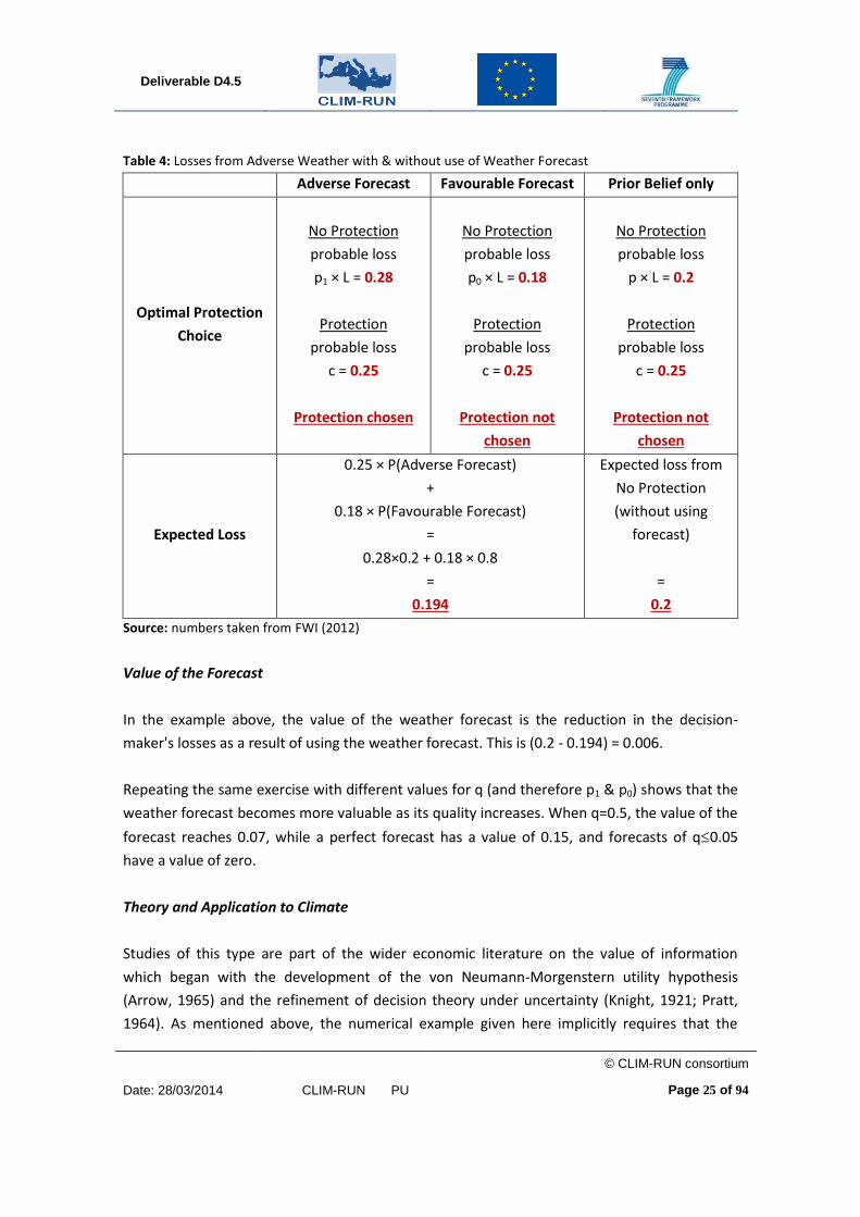
Table 4: Losses from Adverse Weather with & without use of Weather Forecast

Adverse Forecast Favourable Forecast Prior Belief only

Optimal Protection

Choice

No Protection

probable loss

p1 × L = 0.28

Protection

probable loss

c = 0.25

Protection chosen

No Protection

probable loss

p0 × L = 0.18

Protection

probable loss

c = 0.25

Protection not

chosen

No Protection

probable loss

p × L = 0.2

Protection

probable loss

c = 0.25

Protection not

chosen

Expected Loss

0.25 × P(Adverse Forecast)

+

0.18 × P(Favourable Forecast)

=

0.28×0.2 + 0.18 × 0.8

=

0.194

Expected loss from

No Protection

(without using

forecast)

=

0.2

Source: numbers taken from FWI (2012)

Value of the Forecast

In the example above, the value of the weather forecast is the reduction in the decision-

maker's losses as a result of using the weather forecast. This is (0.2 - 0.194) = 0.006.

Repeating the same exercise with different values for q (and therefore p1 & p0) shows that the

weather forecast becomes more valuable as its quality increases. When q=0.5, the value of the

forecast reaches 0.07, while a perfect forecast has a value of 0.15, and forecasts of q0.05

have a value of zero.

Theory and Application to Climate

Studies of this type are part of the wider economic literature on the value of information

which began with the development of the von Neumann-Morgenstern utility hypothesis

(Arrow, 1965) and the refinement of decision theory under uncertainty (Knight, 1921; Pratt,

1964). As mentioned above, the numerical example given here implicitly requires that the

Deliverable D4.5



of 94

decision-maker is rational, risk-neutral and aware of the risks and payoffs from each possible

state of the world.

Several authors have underlined the need for elaborating on the evaluation of the forecast

quality beyond the basic "Cost-Loss model" and its variations. Some studies try to account in

more sophisticated ways for the effects of uncertainty and confidence on the use of climate

information (Wilks 2001).

Aside from the accuracy of climatic information, the value of the information is influenced by

other factors, including the following (Teisberg and Weiher, 2009):

1. Frequency – the climatological probability of the weather event.

2. Severity – the magnitude of the risk or the expected damage that the event could

cause. This in turns depend on vulnerability of a specific location/asset/population

affected by the climatic condition

3. Lead-time – the time between the forecast and the occurrence of the event -

determines the range of protective action that the decision maker has available, longer

lead times means wider range of possible responses and therefor usually smaller

response costs

4. Response costs – the costs of possible responses to the warning;

5. Loss reduction – how much are the expected losses from an adverse weather reduced

given the protective actions – in the example before, by using protective measures

decision maker was able to mitigate the whole loss.

To the best of our knowledge, the current literature does not consider how the application of

valuation techniques such as the Cost-Loss model should differ between short-term, verifiable

weather forecasts and climate information where the spatial resolution and time-scale are

likely to be longer. Studies focus on the benefits of weather or climate information (see

citations throughout this chapter) but we have been unable to identify a theoretical or

empirical comparison between the two.

Under the numerical framework outlined above, we would expect a 'climate' forecast (longer

time horizon, lower spatial resolution) to be less valuable than a standard weather forecast if

the improvement of the forecast over the assumed knowledge of the decision-maker is lower

Deliverable D4.5



of 94

(if p0 and p1 are closer to p). However, the proximity of these three probabilities does not mean

that climate information is intrinsically less valuable, merely that there is greater scope for

improvements in value if improvements in forecast accuracy can be made (such that the

difference in values between (p0 & p1) and p increases). Furthermore, the longer lead time

provided by climate information is a source of value relative to a short-term weather forecast

since this should increase the range and effectiveness of protective options available to

decision-makers.

3.2.Climate Services & User Needs

Climate Services can be defined simply as "climate information prepared and delivered to

meet a user's needs" (WMO, 2011), though several more detailed definitions exist. In order to

understand the socioeconomic value of climate services, is therefore necessary to appreciate

user needs.

Literature has emerged that pays attention to the capacity of potential users to make use of

climate and weather information (Patt et al 2005; Sharma and Patt 2012). For example,

Ziervogel et al. (2010) discuss the need to tailor seasonal climate predictions to user needs in

the case of water resource planning in South Africa, while Weaver et al. (2013) go as far as to

advocate the use of long-term climate models as a scenario-based decision support tool

(rather than the traditional probabilistic approach).

Information value chains

FWI (2012) cites Hooke and Pielke (2000) as having created a simple 3-step model of a climate

information system: where information is produced, communicated, then used.

Production Communication Use

Perrels et al. (2012) further decompose the information into seven value-adding steps from

generation of the forecast to realisation of benefits by the end-user. The value of each stage

depends on the extent to which:

1) weather forecast information is accurate (predict)

2) weather forecast information contains appropriate data for a potential user (predict and

communicate)

Deliverable D4.5



of 94

3) a decision maker has (timely) access to weather forecast information (communicate)

4) a decision maker adequately understands weather forecast information (communicate)

5) a decision maker can use weather forecast information to effectively adapt behaviour (use)

6) recommended responses actually help to avoid damage due to unfavourable weather

information (use)

7) benefits from adapted action or decision are transferred to other economic agents (use)

Perrels et al. (2012) also note that users who are less informed or meteorologically skilled

should derive greater value from the use of weather services. For example, there may be

greater improvement potential in these seven steps for road users (non-professional transport

modes) compared to navigation professionals in aviation and marine industries.

Anaman et al. (1997) and Lazo & Chestnut (2002) refer to the economic theory of public goods

when discussing the value of meteorological (weather & climate) services. According to this

theory, a public good or service is a product that cannot typically be provided in a free market,

despite the social benefits deriving from its production and consumption. The defining

characteristics of a public good are non-excludability (once the good is produced, it is

impossible to prevent anybody from consuming it) and non-rivalry (one person's consumption

does not reduce availability for everyone else). Strictly speaking no climate service can be

considered an inherently public good since it is possible to supply information on an exclusive

basis (e.g. only to subscribers). Nevertheless Anaman et al. (1997) consider public weather

forecasting and disaster warnings provided free-of-charge to be public goods (especially since

such services might not be provided if they relied solely on user payments for finance) while

fee-paying services tailored to specific users' needs (such as those used by the aviation or

mining industries) are considered private goods.

In general there is relatively little data available regarding households' valuation of weather

information (Lazo and Chestnut 2002). Several valuation techniques do however exist and

have been deployed in a commercial context, as outlined in the following section.

Prescriptive and descriptive approaches

A prescriptive approach to valuation (such as that described in Section 3.1) assumes that

decision-makers are rational and capable of maximising their expected utility given the

information available. This is underpinned by the normative theory of decision-making

(because norms are needed to state the objectives against which optimisation takes place). On

the other hand, descriptive models try to model actors' actual behaviour in a decision-making

Deliverable D4.5



of 94

process. As FWI (2012) points out, differences between the two approaches are inevitable due

to their alternative methodological foundations (Hooke and Pielke 2000).

In terms of valuation, prescriptive studies typically use a loss function to evaluate the "best

price" that users should be willing to pay for improved information, given its expected

benefits. Descriptive studies, on the other hand, typically take the form of anecdotal reports &

case studies, user surveys, interviews & protocol analysis, and decision experiments (Lazo and

Chestnut 2002).

Examples include Frei et al. (2012), who use a prescriptive method based around structured

interviews to value the benefit of weather services to users and operators of the Swiss road

network. They identified benefits of around €55m compared to the counterfactual situation

where no forecasting information is available. Klockow et al. (2010) cite a number of

prescriptive and descriptive studies used in the context of agribusiness. On the descriptive

side, these include Hu et al. (2006) and Artikov et al. (2006) who, using both surveys and

regression analysis, find that attitudes and social norms are among the most important factors

influencing forecast use by farmers. The psychological factors affecting actors' use of climate

information is also explored in an experimental setting by Ramos et al. (2013) and Grothmann

& Patt (2005).

Valuation based on stakeholder behaviour

Several of the studies mentioned above survey expert opinion in order to derive the value of

weather and climate information (e.g. Ziervogel et al. (2010), Frei et al. (2012)). FWI (2012)

summarises the main techniques employed to derive a valuation for actors' stated (or

revealed) responses to information availability. These are:

1. Revealed preference. The observable reactions to some relevant information in his/her

decision-making process. Studies that use revealed preference do not exclusively rely

on users' surveys, as their behaviour could be observed indirectly (e.g. change in

consumption patterns). In surveys, respondents are asked about some verifiable

choices they made (e.g. purchases of energy efficient appliances versus standard

appliances).

2. Stated preference. The declared reaction of an expert or user to some relevant

information in his decision-making process.

Deliverable D4.5



of 94

3. Stated value. Surveys try to estimate the maximum amounts people would be willing

to pay (WTP) to receive, or would be willing to accept (WTA) to forgo a specific level or

quality of a service.

Contingent valuation (CV) methods may also be used to evaluate weather and climate services.

These are techniques that use stated value information in hypothetical scenarios to derive the

amount users would be willing to pay/accept for information in certain circumstances.

Regarding the usefulness of CV for weather information, FWI (2012) points out that some

authors are sceptical that survey-based studies or subjective estimates can produce realistic

quantitative estimates. Lazo & Chestnut (2002) point out that in order to derive the likelihood

that values from a stated value or CV study are "true" it is important to clearly define the

commodity to be valued (e.g. weather information) and ensure that participants are aware of

the framework of the hypothetical transaction (e.g. the terms of payment and budget

constraint).

Deliverable D4.5



of 94

4. Evaluating Adaptation across Sectors and Regions

As with impact assessments, multi-sectoral assessments of adaptation are important since

they provide an estimate of the overall feasibility of adaptation, its costs and the extent to

which it is able to prevent climate-related damages from occurring. Moreover multi-sectoral,

and multi-regional assessments are able to compare the costs and/or benefits of adaptation

between activities and locations, providing a signal regarding the optimal use of scarce

adaptation funds.

OECD (2008) describes multi-sectoral adaptation assessment as "a rapidly developing area on

two fronts" (the national/regional and global levels). This section provides an overview of

multi-sectoral adaptation studies at each of these levels.

4.1.Regional and national level assessments

In Europe, national adaptation plans have been developed by a number of EU Member States6

while a number of research projects have begun to investigate the science and policy

implications of implementing adaptation at a more local (subnational) level.

Swart et al. (2009) review the adaptation plans and underlying research base for nine Member

States, identifying three phases of research programme (climate system; impacts; vulnerability

& adaptation). Member States' adaptation plans have been compared and reviewed in a

number of studies. These include the United Nations International Strategy for Disaster

Reduction (UNISDR et al., 2011) who review climate change governance from a disaster risk

reduction perspective and recommend improvements related to the coordination and sharing

of information between authorities across national and administrative boundaries, and

between policymakers and researchers. Similar concerns are raised in reviews of climate

change adaptation governance by Peltonen et al., Biesbroek et al. (2010) and Dumollard &

Leseur (2011). Peltonen et al. cite examples of adaptation policy at national and subnational

from the Baltic Sea region and point out that coherence between adaptation policies and

administrative sectors or political/economic interests is often poor. BiesBroek et al.'s (2010)

review of seven National Adaptation Strategies found that in many cases the role of the

adaptation strategy in implementation and wider governance remained to be defined. Both

studies also highlight the need for improved coordination between science and policy, with

6Fifteen Member States have developed plans according to European Commission,

http://ec.europa.eu/clima/policies/adaptation/what/index_en.htm. Accessed 05/02/2014

http://ec.europa.eu/clima/policies/adaptation/what/index_en.htm

Deliverable D4.5



of 94

Peltonen et al. remarking that "in many cases it is yet uncertain what the localities should

adapt to" and Biesbroek et al. (2010) observing that the governance of climate change is

moving faster than the science, enhancing the difficulty in discussing specific adaptation

options.

One of the first national studies is Holman et al. (2005, 2005a), which provides a multi-sectoral

and integrated assessment of climate change impacts in the UK. They developed a

methodology for stakeholder-led, regional climate change impact assessment, explicitly

evaluating local and regional scale impacts, adaptation options and cross-sectoral interactions

between four major sectors driving landscape change (agriculture, biodiversity, coastal zones

and water resources). A complete standard methodology for costing climate impacts and

adaptation has been provided by the UK Climate Impacts Programme (UKCIP, 2004). Such

methodology has been conceived in order to be applied to a range of sectors (coastal zones,

water resources, agriculture, buildings and infrastructure) at local, regional and national level

in the UK. Resource costs and costs & benefits weighting of adaptation options are both taken

into account. A number of techniques are described in detail for valuing different impact types:

conventional market-based techniques, taking a change in productivity approach (hedonic

analysis, travel cost and contingent valuation methods) or applying cost-based methods

(replacement cost and avertive expenditure techniques) and individual guidelines tailored to

specific types of receptor for non-marketed goods or services (habitats and biodiversity,

human health, recreation and amenity, cultural objects, leisure and working time, non-use

benefits). Some case studies are illustrated as concrete applications of the described

methodology to four relevant issues (water resources, agriculture, flooding and time losses in

the transport system).

At a subnational level, the CIRCLE-2 Climate Adaptation Infobase7 provides details of over

1,400 studies of climate impacts and adaptation undertaken since 2005 in Europe and the

Mediterranean region. In addition, the CIRCLE-Med project has focused specifically on the

Mediterranean region (Santos et al., 2014). Plan Bleu (2011) provides an overview of the needs

for adaptation in the Mediterranean water sector, reviewing the situation in seven

Mediterranean countries. Its recommendations stress the importance of sharing knowledge

between regions, and of comparing the costs and benefits of different types of adaptation

practice – in particular appreciating the role of natural ecosystems in providing ecosystem

services and protection against natural disasters.

7 http://infobase.circle-era.eu/

http://infobase.circle-era.eu/

Deliverable D4.5



of 94

4.2.Multinational Assessments

A number of studies have looked at quantifying adaptation costs and investments at multi-

national and global level. They can be divided into two main groups. The first group uses top-

down models (IAMs) to compute optimal adaptation investment needs at an international

level. These studies are discussed in Section 2.1.1 (Adaptation to Climate Change in IAMs). The

second group ("cost of adaptation" assessments) is discussed in this section. These studies aim

at calculating the cost of a defined level of adaptation (not necessarily the optimum as derived

from a cost-benefit framework) by summing up the costs of specific adaptation measures in

several countries (especially developing countries)

Cost of adaptation assessments 4.2.1.

European Level

There are few multi-country assessments of climate impact explicitly modelling adaptation.

One recent assessment refers to Europe (Ciscar et al., 2009). The PESETA study integrated a set

of coherent climate change projections and physical models into an economic modelling

framework to quantify the potential impacts of climate change on vulnerable aspects of the

European economy: agriculture, riverbanks, coastal areas and tourism. The study also

considers the impacts on human health. All the impact categories assumed some degree of

adaptation, ranging from autonomous or private adaptation in agriculture and human health

(without any explicit costs) to institutional adaptation in tourism and public adaptation in river

floods through protection levels for certain return periods.

Some of the sectoral studies (coastal systems, human health) have taken into account

alternative degrees of adaptation as a way to assess the role of such assumptions in the

results. The human health study has considered the no acclimatisation case, and two other

acclimatisation schemes.

The coastal systems sector study is the only one explicitly considering a cost-benefit module of

adaptation, applying the DIVA model scheme (Nichols, 2007, also see Section 5.4.1). It

estimates that damages without adaptation are around six times higher than with adaptation.

Adaptation consists of beach nourishment and/or dikes. Each measure is undertaken if the

benefits of the measure exceed the marginal cost. For dikes, the benefits consist of lower sea

Deliverable D4.5



of 94

flood damages, river flood damages and costs related to salinisation & migration. For beach

nourishment they consist of the value of the protected land for agriculture or tourism.

The main conclusion of the study is that if the climate of the 2080s would occur today, the EU

annual welfare loss because of the effects in the four market impact categories (agriculture,

river floods, coastal systems and tourism) would be in the range of 0.2% to 1% (see Figure 2).

However, there is large variation across European regions for the four impact categories.

Southern Europe, the British Isles and Central Europe North appear most sensitive to climatic

change. Agriculture impacts, coastal impacts and river flooding are the dominant causes of

welfare loss. The assessment for the coastal systems indicates that adaptation policies can be

particularly cost efficient for this sector.

Developing Countries

Many studies concerning multi-country adaptation assessment have been undertaken in the

context of international development assistance. This is partly due to the importance of

National Adaptation Programmes of Action (NAPAs), prepared by the LDCs under the United

Nations Framework Convention on Climate Change (UNFCCC). NAPAs follow an approach that

focuses on enhancing adaptive capacity to current climate variability and extremes, as this will

in turn help address the adverse effects of climate change (Njie, 2008, Hardee and Mutanga

2010).

OECD (2008) review six multi-sectoral adaptation studies, all of which were conducted for

governmental bodies or international organisations in the context of funding for international

development assistance. Parry et al. (2009) and Fankhauser (2010) named these studies as

“first generation global estimates”. Four of those reviewed by OECD (2008) produce rough

estimates of the cost of "climate proofing" financial flows8 into developing countries by

estimating the extent to which these flows are "climate sensitive". More recently, the World

Bank's EACC study (Economics of Adaptation to Climate Change) (World Bank, 2010) follows a

more bottom-up approach, considering the individual detail of adaptation in a number of

sectors.

Development-oriented studies often use similar methodologies to those used for studies at

regional, national or community level within the EU. For example, EACC makes use of the DIVA

model for estimating flood damages and also employs a variety of stakeholder engagement

8 The financial flows are Official Development Assistance (ODA) & concessional finance, Foreign Direct

Investment (FDI) and Gross Domestic Investment (GDI).

Deliverable D4.5



of 94

techniques in individual country case studies. One key difference is that the development-

oriented flows have an emphasis on calculating the (foreign) funds required to compensate for

the impacts of climate change. There is therefore the implication that these expenditures have

zero opportunity cost from a recipient's point of view (i.e. additional funds should enter the

economy to compensate for climate change). In a European context, where no foreign

contribution to adaptation is foreseen, adaptation funds must compete for domestic funding

with other expenditures.

Deliverable D4.5



of 94

5. Overview of Sectoral Climate Change Impacts

This section of the report reviews the literature concerning bottom-up assessments of climate

impacts. It pays particular attention to energy, forest fires and tourism — the sectors

examined in the case studies in Sections 6, 7 & 8. Other sectors covered are coastal impacts,

river floods, human health, biodiversity & ecosystem services, and agriculture.

5.1.Energy

Climate change may generate disturbances in both the demand and the supply side of the

energy sector. Such disturbances are associated with notable costs (and sometimes benefits)

that strongly depend on the energy sector and regional climatic trends.

On the energy supply side, there has been recently a great deal of focus and concern regarding

future performance of thermal power plants. This type of power plant uses nuclear energy,

fossil fuels or biomass to produce electricity. The thermodynamic process involved in the

production of electricity relies heavily on the supply of cooling water which in most cases is

assured by nearby river flows. The current concern is that climatic changes might reduce river

run-off in certain regions of the world threatened by drought which would force power plants

to operate at reduced capacity. In addition, many countries have implemented strict

regulations to protect river ecosystems by setting a limit to the maximum temperature at

which it is permissible to return cooling water to rivers. This negatively affects the

thermodynamic efficiency of thermal power plants which could furthermore be perceptibly

altered by ambient temperatures changes as a consequence of climatic change (Van Vliet et

al., 2012; Klein et al., 2013). Current methodologies that assess this impact make use of

detailed data on plant location, cooling system types, surface temperature and river runoff

(e.g. Van Vliet et al., 2012). The main challenge consists in (finding and) linking information

from hydrological models with surface temperature and air moisture data from climate models

and power plant specificities at high temporal and spatial resolution (daily river flows, dry bulb

temperatures).

Climatic changes also have a considerable impact on the production of renewable energy. For

example, changes in river run-off due to altered precipitation rates directly affect hydropower

generation. The relationship between precipitation and electricity output is not linear and

varies from region to region because in addition to precipitation rates other important factors

Deliverable D4.5



of 94

come into play such as evaporation rates, soil saturation, ground morphology, topography,

erosion processes, land-use changes, deforestation, etc. In order to capture the intricate

relationships between regional climate changes, the response of the Earth system and the

impact on hydropower generation, the results form high resolution regional climate models

coupled with detailed hydrological models are needed. Lehner et al. (2005) use a combination

of two climate models and the WaterGAP model to nexamine changes in average runoff. They

find that by the 2070s, runoff can be expected to fall in most of Europe, by as much as 25% in

the South (especially Spain, Romania, Bulgaria and potentially Italy and the Balkan states).

However, runoff is expected to increase in the North (Scandinavia, Scotland and the Baltic

states). Gaudard & Romerio (2013) provide a more detailed summary of the impacts of climate

change on the hydropower sector.

Similarly, biomass production is affected by climatic changes in different ways. A tendency

towards more frequent heat waves for example can lead to the destruction of biomass stock

through forest fires; increased precipitation and other extreme weather events may lead to

losses through floods, etc. In this case too, high resolution data from climate models coupled

with outputs from agricultural land-use and forestry models are needed in order to make

projections on the evolution of biomass potentials and use.

The climate change impact on electricity production from wind and solar technologies can be

assessed using comparatively few climate parameters such as wind speed, or irradiance.

However, in these cases as well, results are sensitive to the quality of the climate data at high

spatial and temporal resolution. To date, consistent resource potential data sets are available

with detailed full load hour information for solar PV, CSP and wind technologies.

To calculate the evolution of solar energy potentials, hourly direct normal irradiance (DNI) and

global tilt irradiance (GTI) data derived from climate model outputs are necessary. To have an

idea about the level of detail needed from climate models in order to obtain realistic

assessments on climate impacts it is useful to consider state of the art methodologies to

calculate historical potentials. A research group at the Potsdam Institute for Climate Impact

Research (PIK) provided (in the framework of the on-going FP7 project ADVANCE9) country-

based potentials for solar PV and CSP technologies. The estimates were built on NASA SRB 3.0

data containing 3-hourly global horizontal irradiation (GHI) data on a 1° grid. The data from

NASA was modified and downscaled to 1-hourly data on a 0.45° grid using a clear sky model by

the Deutsches Zentrum für Luft- und Raumfart (DLR). Direct normal irradiance (DNI) data was

then derived from the GHI data, using empirically fitted relationships between the ratios direct

/ diffuse radiation on the one hand and Clearness Index / optical air mass on the other hand.

9 See http://www.fp7-advance.eu/

Deliverable D4.5



of 94

Regarding wind resources, the estimates consider wind speed at different heights and per

surface unit. Recently the US National Renewable Energy Laboratory (NREL) has assessed

worldwide wind energy potentials using hourly wind speed vectors on a 40km grid10

. While

historical wind speed data is available (e.g. CFDDA reanalysis tool of US NCAR), it is unrealistic

to expect results at this level of detail from climate models. It is thus crucial to develop

appropriate methodologies in order to downscale climate model data to match with input

needs for energy and impact assessment models.

Noteworthy is the fact that in both cases, wind and solar, regional parameters are used to

exclude certain zones from the land area suitable for the development of these technologies.

Most of the spatial exclusions take into account infrastructures, land-use and agricultural

terrain but also climatic factors such as snow cover, permafrost, sea-ice cover, bathymetry,

etc. Assessing future resource potentials of solar and wind energy is thus also based on

evaluating the consequences of the interplay between all these parameters.

These are just a few examples of how climate change may affect the production and supply of

energy: many more can be cited. The increasing occurrences of extreme weather events such

as floods, forest fires and hurricanes can cause huge losses to energy infrastructure and

production sites that were not built to withstand their destructive forces. The infamous case of

hurricane Katrina is a grim reminder of the devastating consequences that this event had on

the global oil market. Similarly, electricity transmission and distribution networks are likely to

face a greater risk of disruption caused by increased wind storms and lightning strikes. Alluding

to a different cause of concern related to future climate change, hundreds of thousands of

kilometres of oil and gas pipelines and production sites in Siberia supplying important sources

of energy to Central Europe may be affected by the potential melting of permafrost due to a

global temperature increase. New shipping routes have already been opened as a

consequence of melting ice sheets in the Arctic Sea.

All of these changes are expected to engender important social costs and need special

attention from stakeholders and policy makers who are in the process of shaping the future of

the energy sector and designing climate adaptation strategies.

Finally, climatic changes have the potential to affect energy consuming sectors such as

households, public buildings, industries and transportation. In the residential sector for

10

This information is derived from NREL work on USA wind potential, and has been made available for

the FP7 project ADVANCE. See for instance presentation by Patrick Sullivan at the EMF meeting held in

US Colorado, 22 July 2013: http://emf.stanford.edu/files/docs/340/Patrick_Sullivan_7.22_AM.1.pdf

Deliverable D4.5



of 94

example, an increased use of air-conditioning in summer is expected to accompany rising

temperatures and decreased rainfall, such as might be expected in the Mediterranean region.

Such a tendency would be exacerbated if these changes in demand occur over the same period

as the energy supply constraints mentioned above. Furthermore, under a warming climate

scenario, the tendency towards milder winters in the same regions would imply a reduced

need for space heating, although this effect would probably be observed to a lesser extent in

certain regions of the Mediterranean such as mountain areas for example (Dowling, 2013;

Isaac and Van Vuuren, 2009; McNeil and Letschert, 2007; Mima and Criqui, 2009).

5.2.Forests and Ecosystems

In the dedicated case study (Section 7) we examine the influence of climate change on the risk

of forest fires in the Mediterranean. Landau (2010) identifies three more general impacts of

climate change on forests:

Affects to net primary productivity (NPP) – NPP is measurement of plant growth

obtained by calculating the quantity of carbon absorbed and stored by vegetation;

Changes to forest distribution and composition;

Changes to the frequency and intensity of forest disturbances such as fires and insect

outbreaks.

In the context of the MOTIVE project, Kolström et al. (2011) summarised the likely effects of

climate change on European forests (see Table 5). In the same project, Fitzgerald & Lindner

(2013) identify wind to be more important as a damage source in Northern and Western

Europe; while fire is more important in the Mediterranean; bark beetles in Atlantic temperate ,

Alpine and Mediterranean forests; and fungi & wildfire in mountain and boreal forests.

Deliverable D4.5



of 94

Table 5: Selection of Climate Impacts and Adaptation Options in Different European Forest Types

Forest Type Expected Impact Adaptation Options

Boreal Enhanced forest growth

Reduced winter hardening

Increased abiotic damages (e.g. storm damage)

Better harvesting techniques on non-frozen soils

Temperate Oceanic Changes in storm, insect and pathogen disturbance regimes

Shifts in tree species compositions

Adapt the management to an increased disturbance risk

Temperate Continental Vulnerability of trees to frost increasing

Forest fire risk increases

Risk of pest outbreak increases

Improve fire risk management and adjust afforestation techniques

Mediterranean Drought stress increasing

Forest fires become a greater threat

Threat of desertification and soil loss

Fuel management and the modification of stand structure to reduce fire risk

Mountainous Regions Tree line shifts upwards

Forest fire risk line increases

Promote small-scale management and maintain the forest cover to secure its protective function against natural hazards and erosion

All regions Adjust thinning & harvesting to changing forest growth patterns

Select well-adapted species or provenances at regeneration and favour them at tending and thinning stages

Source: Kolström et al. (2011)

On ecosystems more generally, progress has been made in recent years on ecosystem service

evaluation, notably through the Economics of Ecosystems and Biodiversity (TEEB) project

(TEEB, 2010). Reports produced by the TEEB project itself represent methodological guides for

the study or management of ecosystems (e.g. Beaudoin & Pendleton (2012) on oceans, or

TEEB (2012) which provides a framework to policymakers for valuation of ecosystem benefits).

Deliverable D4.5



of 94

Also in the context of the TEEB project, Van der Ploeg & de Groot (2010) developed a database

of ecosystem valuation studies consisting of over 1,350 datapoints from over 300 case studies

(a datapoint is a piece of information such as the estimated value of a specific ecosystem

service expressed in Euros per hectare per year).

5.3.Tourism

The relationship between tourism and climate change in the CLIM-RUN project is examined in

a number of case studies, with particular focus on the Mediterranean region. In particular,

Dubois et al. (2014) investigate ways of improving the Tourism Climate Index in the region,

while Section 6 of this document uses the Hamburg Tourism Model to investigate the effect of

future climate on tourist numbers and expenditure. This section provides a more general

overview of the literature on how climate change may affect the tourism sector.

Cai et al. (2011) and Nickerson et al. (2011) note that quantity of literature discussing how

tourist flows respond to a changing climate has increased in the past decade (from around

2005). However, there is earlier literature on the relationship between tourism and climate,

examined by Scott et al. (2005).

Scott et al. (2012) review the key risks for international tourism from climate change, dividing

the literature into the following categories:

Altered Geographic & Seasonal Demand: including the degree to which a bundle of

climate indicators (e.g. a Tourism Climate Index) influence choice of destination and

substitution between domestic (home-country) and international tourism.

Risks to Winter Sports Tourism: balancing the risks of less favourable snow conditions

with the potential for adaptation, especially through snowmaking.

Sea level rise and Risks to Coastal Tourism: coastal tourism has been identified as the

largest tourism activity segment globally. Assets such as beaches, cultural heritage

resources and infrastructure are at risk from sea level rise, while beach nourishment is

among the adaptation measures available.

Risks to Nature-based Tourism: the extent to which degradation or disappearance of

natural attractions (e.g. glaciers, coral reefs, rainforest, wildlife) result in reduction or

displacement in tourist flows.

Nickerson et al. (2011) conducted a scan of the academic literature on climate change and

tourism, identifying 220 published works, of which around half deal with the impact of climate

Deliverable D4.5



of 94

change on tourism (including subjects such as destination choice and impacts in specific areas

such as mountains and oceans). In general they find that tourist destinations will be expected

to shift in space and time. Popular tourist destinations may change if ideal climatic conditions

occur closer to the poles than at present (Amelung et al., 2007). Destinations may also receive

fewer visitors in (hotter) summer and (less snowy) winter months, but greater visitor numbers

in the spring and autumn (Ceron & Dubois, 2005; Nicholls, 2006).

The scan also cites numerous studies investigating the impacts and scope for adaptation in

mountainous regions, particularly those where winter sports are currently favoured (Beniston,

2003 and Bark et al., 2010 amongst others). It also identifies studies proposing specific areas

that could benefit from climate change. For example, Ceron & Dubois (2005) suggest that

French Mediterranean beaches may benefit from climate conditions that are cooler than those

further South. In addition, Jones et al. (2006) predict that climate change will cause visitor

numbers to Ontario (Canada) national parks to increase in the period to 2050, based on

multiple regression analysis. Other studies highlight the (two-way) interactions between

climate change, tourism and environmental degradation. For example, Kent et al. (2002)

examine water scarcity in Mallorca, noting that this is exacerbated by tourists, and may be

exacerbated further by climate change directly (drier conditions) or indirectly (if a changed

climate attracts more tourists).

5.4.Other Sectors

Coastal Impacts 5.4.1.

According to EEA (2012), the coastal sector is the most studied impact type to date, in Europe

at least. Studies of the socioeconomic implications have been undertaken at various scales (see

Nicholls et al., 2007 for a review of earlier studies).

Studies have been undertaken at global level (Hallegatte et al., 2013; Hanson et al., 2011;

Nicholls et al. 2010); regional level (Dasgupta et al., 2011 for developing countries); and

subnational level (Ranger et al., 2011 for Mumbai; Hallegatte et al., 2011 for Copenhagen). In

addition European level studies have undertaken as part of the ClimateCost and PESETA

projects.

At European level, the research projects PESETA (Richards & Nicholls, 2009) and ClimateCost

(Brown et al., 2011) employ the DIVA model (Hinkel & Klein, 2009; Hinkel et al., 2010).to

Deliverable D4.5



of 94

estimate the costs of SLR and related impacts at EU level for the period up to the 2080s. The

projects produce comparable results from similar, but not identical, input choices such as the

extent of SLR (in metres), socioeconomic & emissions scenarios, and climate models. PESETA

estimates a cost of coastal damages without adaptation by the 2080s of between €10.3 billion

and €44.6 billion (compared to €8.5 billion without SLR). The lower bound estimate reflects an

IPCC B2 scenario with 6 cm11 of relative sea level rise (RSLR) in Europe, while the upper bound

reflects IPCC A2 scenario with 67 cm of RSLR. For the same period, ClimateCost estimates mid-

range damages of €25.4 billion for an A1B scenario12 and €17.4 billion for an E1 (mitigation)

scenario13 (E1 refers to a scenario where temperature rise is limited to 2°C).

Adaptation to Sea level rise

A reference study on the costs of adaptation to SLR is the analysis carried out by Nicholls

(2007), which estimates total investments at a global level in two adaptation measures (beach

nourishment and sea dike construction) to protect coastal areas and infrastructure. The

analysis is made with the DIVA model, combining a global database on coastal zones with a

suite of specific algorithms. The optimal adaptation decision is based on cost-benefit analysis

and balances avoided damages against adaptation costs, with assumptions on sea level rise

and socio-economic trends reflecting the IPCC SRES scenarios. Results showed that investment

needs will vary from around $14 to 22 billion per year for the year 2030. The difference in

costs reflects different climate scenarios. However, this difference is not due to differences in

the impact of sea level rise in 2030, but is due the differing requirements for proactive

adaptation (with long lead times) in order to avoid climate change in the more distant future.

River floods 5.4.2.

Globally, as well as at European level, damages from river flooding have been increasing over

time, with damages being influenced by socioeconomic trends (e.g. propensity to develop on

floodplains) as well as climate (Kundzewicz et al., 2010). At European level, the estimated

damages from increases in river flooding under future climate scenarios have been estimated

in work related to the ClimateCost project (Feyen et al.,2011; Rojas et al., 2013). At national

level, similar studies include Dumas et al. (2012) for France and Wilby et al. (2008) for the UK.

11

The same study considers medium RSLR to be 26 cm by the 2080s. 12

with €19.3-37.2 billion covering a 90% range of SLR expectations, and damages of €7 billion without

SLR 13

with €15.8-€20.1 billion covering a 90% range

Deliverable D4.5



of 94

The headline finding of Feyen & Watkiss (2011) and Rojas et al. (2013) is that in the absence of

adaptation14, expected mean annual damages should reach €98 billion by the 2080s15 (see

Figure 5). This compares to expected damages of under €50 billion in the absence of climate

change and to current damages of €5.5 billion (the difference being due to socioeconomic

trends increasing the total value of assets at risk). Furthermore, the climate change scenario

has a much wider range of outcomes, with damage estimates between (twelve) GCM/RCM

combinations ranging from around €59-200 billion, compared to €45-55 billion with only

socioeconomic change.

Adaptation, in the form of upgrading protection to future 100-year flood levels is expected to

reduce expected damages to €53 billion. Having reviewed the literature on costs and benefits

of adaptation, Rojas et al. (2013) suggest that flood protection investments typically have a

benefit-cost ratio of 4:1. On this basis, the annual cost of adaptation (protecting against a

future 100-year event) is estimated at 0.07% of GDP on average for EU Member States. This

ranges from 0.01% (Sweden) to 0.71% (Slovenia), though absolute costs are highest for the UK

(€2.4 billion), France (€1 billion) and Italy (€0.9 billion).

14

"Adaptation" being improvements in protection beyond current standards – which are assumed to

protect against a present day 100-year event. 15

Under an A1B scenario

Deliverable D4.5



of 94

Figure 5: EU27 EAD from floods in billions of Euros for baseline period (1961-1990), 2000s (1981-2010),

2020s (2011-2040), 2050s (2041-2070) and 2080s (2071-2100) for the A1B scenario based on LISFLOOD

simulations driven by 12 regional climate models (all numbers in constant 2006 prices, undiscounted),

assuming no adaptation. The entries per time period relate to the first three rows in Table 2, the

marginal change represents the final row.

Source: Feyen & Watkiss (2011)

Human Health 5.4.3.

The impacts of climate change on health can be divided into two main types, with several

subcategories (Landau, 2010; Kovats et al., 2011):

Direct impacts from climate variability:

o Cold weather impacts (may decrease mortality)

o Hot weather impacts (may increase mortality)

o Storm and severe event impacts (increase in accidents and deaths)

Indirect impacts from changes in disease distribution:

o Food-borne diseases (increasing summer temperatures may increase

incidence of food poisoning)

o Water-borne diseases (e.g. cholera)

Deliverable D4.5



of 94

o Pest/vector borne diseases (e.g. Lyme disease, tick-borne encephalitis,

malaria, visceral leishmaniasis, vibriosis)

o Outdoor air pollution

o Risks to health infrastructure and other critical infrastructure from extreme

weather events.

Under the ClimateCost project (Kovats et al., 2011), quantitative estimates were derived at

European country level for the heat-related mortality, food borne diseases, coastal flooding

and labour productivity under A1B and E1. These impacts are summarised in Table 6, which

shows the marginal impact of climate change16 by the 2080s.

Table 6: Identified Health Impacts of Climate Change from ClimateCost study:

EU27, annual figures during period 2071-2100

A1B E1

Heat Deaths per year - no acclimatisation

126,727 69,899

Heat Deaths per year - with acclimatisation

39,705 17,641

Salmonellosis cases 9,319 – 16,915 5,709 – 10,407

Coastal flooding fatalities 621 158

Economic cost of labour productivity reduction (€ million)

297 - 743 61-145

Source: Kovats et al., 2011

Notes:

Figures refer to 2080s. Unit are number of cases (except labour productivity)

For salmonellosis cases, lower bound assumes current trend of declining incidence (due to better food regulation practices) continues

For labour productivity, lower bound indicates reduction in intensity of workload in Southern Europe (less manual labour, more services), converging with current intensity in North West Europe

The figures for heat death are obtained using an econometric function that equates deaths in

specific age groups per degree Celsius in excess of a threshold (29.4°C in the Mediterranean

and 23.3°C in Northern Europe). Under this framework, mortality is greatest in Italy, Germany,

France and Spain (see Figure 6). If acclimatisation is assumed (every 30 years an additional

0.5°C is tolerated), the increase in heat deaths due to climate change falls to 40,000 in A1B

(18,000 in E1).

16

additional impact including climate and socioeconomic change less additional impact with

socioeconomic change only

Deliverable D4.5



of 94

Figure 6: Annual Heat Mortality (number of cases, compared to baseline climate (1961-1990)), for the

2020s (2011-2040), 2050s (2041-2070) and 2080s (2071-2100) for the A1B scenario (ensemble mean).

No acclimatisation.

Source: Kovats et al. (2011)

Monetisation of Health Impacts

The ClimateCost study also places a monetary value on the identified morbidity and mortality.

For heat deaths, Value of Statistical Life (VSL) and Value of Life Years (VOLY) methodologies are

both considered. This places the additional annual cost of climate change at €147 million in the

2080s for A1B (€81 million for E1) under VSL. However, under VOLY this increases to €4.0

billion and €2.2 billion respectively. These estimates are based on an assumed value of €1.16

million per prevented fatality and VOLY of €63,000, with an assumed 0.5 years of life lost per

heat related deaths. For salmonellosis, a value of €3,500 - €7,000 per case is assumed, which

accounts for treatment costs, opportunity costs and disutility. This produced an estimated cost

of €49–89 million per year for A1B and €30-55 million for E1.

A critical review of the different methodologies available for valuing climate change health

risks is provided by Markandya & Chiabi (2009). The VOLY methodology (or the QALY, which

also accounts for quality of life in each year) is intrinsically more attractive than VSL since it

takes account explicitly of the life time lost. However, it is also more challenging given the

need to calculate robust values for the amount of time lost per death, as well as a monetary

value for each year lost. As a result, VSL methods appear to be more common in the literature

(see Ščasný & Alberini, 2012; Braathen et al., 2009)

Deliverable D4.5



of 94

Agriculture 5.4.4.

The projected impacts of climate change on European agriculture are summarised in EEA

(2012). Though impacts will vary across the continent, it is expected that productivity will

increase in Northern Europe due to a longer growing season and the opportunity to grow new

crop varieties in regions where crop production is not limited by water scarcity. However, in

Southern Europe, productivity is likely to be harmed by extreme heat events and reduced

water availability, leading to the winter cultivation of some crops that are currently grown in

summer.

For example, Figure 7 shows projected changes in water-limited crop yield across Europe in an

A1B climate scenario for the 2050s. The importance of water as a limiting factor in agricultural

production is likely to be particularly acute in Mediterranean regions for a number of reasons.

Firstly, higher temperatures and lower humidity are likely to increase the evaporative demand

of plants by a greater degree than the offsetting effect of increased CO2 concentration (Olesen

et al., 2007).

Figure 7: Projected Water Limited Changes (%) in Crop Yield

Source: EEA (2012) Notes: mean relative changes in water-limited crop yield simulated by the ClimateCrop model for the 2050s compared with 1961–1990 for 12 different climate models projections under the A1B emission scenario.

Deliverable D4.5



of 94

In terms of stakeholder interaction, there exists a fairly wide body of literature on farmer

behaviour (often employing the Theory of Planned Behaviour) though little dealing with

adaptation to climate change specifically. For example, Hu et al. (2006) demonstrate the

importance of psychological barriers and social norms in determining farmers' use of weather

forecast information. Similarly OECD (2012) investigated farmer behaviour in the context of

climate change and gave four recommendations which involved understanding farmers'

behaviour in a local context, appreciating the insights from behavioural science (such as

"nudging") and suggesting that adaptation strategies involving collective action and

cooperation among farmers are likely to be more successful than an individualistic approach.

Deliverable D4.5



of 94

6. Case Study: Mediterranean Tourism

In this section we investigate the effects of climate change on tourist flows in the

Mediterranean region during the 21st century. The study considers an A1B climate scenario

and uses the Hamburg Tourism Model (HTM), which includes temperature as one of its

determinants of tourist flows.

We consider the effect of climate change on (domestic and international) tourist arrivals at

country level for 22 Mediterranean countries. In addition we use regional downscaling to

consider the same effects for 16 subnational regions spread across Croatia, France and Tunisia.

Results suggest that, other things being equal, by 2100, tourist numbers in most of the

downscaled regions may decline by 20-38% compared to a counterfactual without climate

change. Compared to other tourism analysis carried out within the CLIM-RUN project this

section adds value by considering the interplay between domestic and international tourism.

It should be noted that climate change in the countries outside the region (not considered

here) could also have an important effect by influencing the destination choice of both

domestic and foreign tourists. This would therefore constitute useful additional information

for tourist industry stakeholders. Furthermore, the results should be treated with some

caution since they show the effect on tourist flows of mean annual temperature per zone (a

single annual variable), thereby failing to account for the geographical concentration of

tourists within each zone and for changes in seasonal temperatures. Furthermore,

temperature is not the only determinant of tourist comfort. For example a composite

measure, such as the Tourist Climate Index, would give a broader picture.

6.1.the Hamburg Tourism Model

Most impact studies on tourism and climate change focus on particular countries or on specific

types of tourism, while analysis at the global level is often overlooked. This has two main

drawbacks. On one hand, the substitution effect between different countries is not taken into

consideration. On the other hand, domestic and international tourism are often grouped into a

single category, thus disregarding the differences in behaviour and the substitution effects that

may arise between domestic and international destinations in the decision process of the

tourist.

Deliverable D4.5



of 94

The Hamburg Tourism Model (HTM) filled some of the gaps mentioned above, by feeding data

from different countries and regions into a simulation model that reproduces the flows

between 207 destinations and countries of origin. Scenarios accounting for economic growth,

population dynamics and, of course, climate change were used to simulate tourist flows'

changes over the course of the twenty-first century - with and without climate change.

Population growth and per capita income are derived from scenarios taken from the Special

Report on Emissions (SRES) of the Intergovernmental Panel on Climate Change (Nakicenovic

and Swart, 2001) and implemented in version 2.2 of the Image model’s integrated assessment

of global scale changes17. The simulations of the original SRES were conducted for 17 world

regions and the rates of growth of the countries of each region were considered to be equal to

the rate of growth of their reference area. Climate change simulations were derived from the

model Fund18 (Tol, 1999) and the Cosmic model (Schlesinger and Williams, 1998).

Results of the HTM simulation model were presented for the first time in 2005 (Hamilton et al.,

2005). Other developments have led to the inclusion of domestic tourism, tourist spending and

length of stay (Bigano et al., 2007a) . The Hamburg Tourism Model simulates both tourism

demand generated by each country, and the demand for tourism at various destinations. The

model estimates the total demand for travel using data on population and per capita income

of each country, and then the ratio of domestic to international tourists on the basis of per

capita income, the national land area, coastline length and mean annual temperature at each

destination. The model then identifies the destinations of international tourism by means of a

matrix of bilateral tourist flows between all countries and regions considered.

The projections of tourism flows over the twenty-first century have been carried out on the basis of simulations of changes in population and income, in the absence and in the presence of climate change. Income and population affect both supply and demand of tourism. On the supply side, these simulations result in changes in the attractiveness of tourist destinations. On the demand side, these scenarios have implications in terms of total number, in each country of origin, of individuals willing to engage in tourist activities. The model simulates the flow of tourists in five-year intervals over the course of the XXI century, but it can also simulate past periods thus allowing the validation of the results by comparing the actually observed data and the data estimated through simulations 19.

In absence of climate change, the model predicts that, as population increases, each country

will increase the number of its outgoing tourists, while with both population and GDP growing,

17

Netherlands Environmental Assessment Agency http://themasites.pbl.nl/tridion/en/themasites/image/ 18

http://www.fund-model.org/ 19

Bigano et al. (2007a) discuss the issue of validation for the HTM models and find that (p.34): “The

correlation between observed and modelled international arrivals in 1995 is almost perfect, because that is

the year of calibration. For the other years, the correspondence between observations and modelled values

is never below 92%”.

Deliverable D4.5



of 94

the number of both outgoing and ingoing tourists will grow (since more financial resources

mean, ceteris paribus, more resources for the tourist sector as well, and hence better ability to

attract foreign tourists). Since the economic growth will not be uniform across world countries

in the future, these changes will result in variations in the market shares of individual

countries. In the absence of climate change, the model estimates that both domestic and

international tourists from countries currently leading the tourist market, including European

countries, Japan, Australia, New Zealand, USA and Canada will decline gradually over the

twenty-first century in absolute terms, while Asian countries will see their share increase.

The model compares these projections in the absence of climate change with the effects of

climate change under four different SRES scenarios. As an illustration, we briefly discuss the

results of the A1B scenario, i.e. the one with the lowest population growth, but characterized

by strong global economic growth. The interested reader is referred to Bigano et al. (2007a,

2007b) for the overall results. Under such a scenario, the Mediterranean countries, including

the CLIM-RUN tourism case studies (Croatia, France, Tunisia and Cyprus), are penalised. The

last two suffer the most severe impacts, being part of (or close to) the world’s most severely

impacted regions, such as Africa and the Middle East. On the other hand countries where the

climate is not currently seen as one of the main local attractions, such as Canada and Russia,

may be visited by many more tourists (again, in relative terms with respect to the no climate

change scenario).

Deliverable D4.5



of 94

Figure 8: Climate change impact on tourism in the Mediterranean and Portugal in 2100 in HTM (%

change compared to the value in the absence of climate change). Domestic tourists

Figure 9: Climate change impact on tourism in the Mediterranean and Portugal in 2100 in HTM (%

change compared to the value in the absence of climate change) International tourists (from any

country of origin worldwide)

Figure 8 and Figure 9 illustrate, respectively, the impact on domestic tourists and international

tourists in Mediterranean countries. From their comparison, the different dynamics of

domestic and international tourists are apparent: As temperature rises in a given country

domestic tourists tend to increase in relative terms. These are former international tourists

from that country, who used to travel to warmer destinations which have become excessively

hot under increased temperatures, and thus prefer to revert to domestic tourism instead.

Note that domestic tourism is also sensitive to temperature increases, and it can actually

decrease due to higher temperatures. This is the potential outcome for some North African

-20 -10 0 10 20 30 40

AlgeriaIsrael

TunisiaMaltaLibya

CyprusSyria

MoroccoEgypt

GreeceTurkey

Serbia & MontenegroLebanon

SpainPortugal

FranceMonaco

ItalyAlbaniaCroatia

Bosnia & HerzegovinaSlovenia

percent change

-60 -50 -40 -30 -20 -10 0 10

AlgeriaSerbia & Montenegro

LibyaEgypt

TunisiaIsraelMalta

CyprusMorocco

SyriaLebanonPortugal

GreeceMonaco

SpainItaly

AlbaniaCroatiaFranceTurkey

Bosnia & HerzegovinaSlovenia

percent change

Deliverable D4.5



of 94

and Middle East countries in the A1B scenario shown here - including Tunisia and Cyprus. The

strongest effect is however the one on international tourists, which will increasingly prefer

milder destinations to the Mediterranean ones.

6.2.Regional Downscaling

The available background data do not allow a full simulation at the subnational and provincial

level for each country in the model. This poses some issues if one intends to draw lessons from

the HTM model for our case study destinations, which, with the exception of Cyprus, entail a

much smaller area than the one covered by the HTM model’s national resolution, and may

have different characteristics from those holding on average at the national level.

However, an extension of HTM to a simplified regional model was produced for the United

Kingdom, Germany and Ireland (Hamilton and Tol, 2007) and Italy (EURAC, 2007). These

simulations were derived by applying a methodology for downscaling of the HTM model

results nationwide that splits the national figures for international arrivals and domestic

tourists between the various sub-national jurisdictions in a manner consistent with the

assumptions of the model. A detailed description of the downscaling methodology can be

found in Hamilton and Tol, 2007 (to which, for economy of space, the interested reader is

referred). In a nutshell, it amounts to allocate tourist numbers projections generated by HTM

across local jurisdictions, on the basis of the same statistical relationships used in the model

between said numbers and temperatures, but calibrated on the values of these variables in the

base year at the local jurisdiction level, and taking into account the differences between

domestic and international tourists. In the remainder of this section, the application of this

methodology to the CLIM-RUN case study locations will be described and the results will be

briefly discussed.

Data on domestic and international tourist numbers at the provincial level in Croatia, Savoie

and Tunisia in 2010 have been gathered from various local statistical sources. Cyprus was

already a national destination in the HTM model, and therefore the HTM results for this

country did not need further downscaling. Tourist numbers in the base year and observed

mean temperatures are shown in Table 7. It should be noted that Savoie differs from the other

regions in that it has a much lower average temperature, and winter sports play an important

part in its tourist market. Since the methodology of this study considers only average annual

temperatures, the results for Savoie should be interpreted with this caveat in mind.

Deliverable D4.5



of 94

Table 7 Characteristics of case study provinces, 2010, (various sources20

)

Foreign Domestic

Average of

Temperature

in 2010 ( °C) Provinces Tourists

Share of

national

total Tourists

Share of

national

total

Croatia

Primorje-Gorski 1843450 17% 307668 21% 14.6

Lika-Senj 369345 3% 34615 2% 15.0

Zadar 811383 8% 159709 11% 15.6

Istria 2467286 23% 160632 11% 14.5

France

Savoie 881226 3% 3280278 4% 2.3

Tunisia

Tunis-Zaghouan 502516 7% 36648 7% 19.5

Nabeul-Hammamet 1228351 18% 89583 18% 19.8

Sousse-Kairouan 1448332 21% 105626 21% 21

Yassmine Hammamet 587042 9% 42812 9% 19.8

Monastir-Skaness 713297 10% 52020 10% 20.2

Mahdia - Sfax 418573 6% 30526 6% 20.2

Jerba-Zarzis-Gabès 1646225 24% 120058 24% 21.6

Gafsa-Tozeur 193759 3% 14131 3% 22.6

Sbeitla -Kassrine 7 0% 0 0% 19

Bizerte-Bèja 35615 1% 2597 1% 18.4

Tabarka-Ain Draham 122451 2% 8930 2% 18.5

In order to account for the uncertainty in regional climate projections, the downscaling of HTM

results has been performed on the basis of mean annual temperature projections (under the

A1B SRES scenario) of a suite of 10 different regional climate models (CNRM, KNMI,SMHI-BCM,

SMHI-ECHAM5, SMHI-HadCM3, C4I, HadRCM, DMI-ARPEGE, DMI-ECHAM, ICTP) with a spatial

resolution of 25 km provided by CNRM-Météo France21. For economy of space, Figure 10-

Figure 12 below show models’ average results in terms of percentage deviations from a no

climate change scenario, but individual model results are available from the authors upon

request. The standard deviation across model results is however quite modest for most

provinces (ranging from 0.06% to 15%, but mostly around 1-2%). Note that the inter-model

variability would be greater if considering seasonal changes or, in particular, rainfall changes

20

For Croatia: Statistic yearbook, Republic of Croatia, 2011. For Savoie:DGCIS,

(www/dgcis.gouv.fr/tourisme). For Tunisia, GREVACHOT), 21

The author is grateful to Clotilde Dubois for her kind help with providing these climate projections

from the ENSEMBLES project.

Deliverable D4.5



of 94

rather than mean annual temperature. Figure 10 focuses on domestic tourists, Figure 11 on

international arrivals and Figure 12 on total tourist presences.

Figure 10: Domestic tourist visits per region. Percentage variation under SRES A1B scenario (averaged over 10 RCM simulations) with respect to no climate change. Domestic tourists are those from any region of origin within the same country. Provincial downscaling of HTM tourist projections for case study locations.

Figure 11: International tourist visits per region. Percentage variation under SRES A1B scenario (averaged over 10 RCM simulations) with respect to no climate change. International tourists are those from outside the same country. Provincial downscaling of HTM tourist projections for case study locations.

Deliverable D4.5



of 94

Figure 12: Total tourist visits per region. Percentage variation under SRES A1B scenario (averaged over 10 RCM simulations) with respect to no climate change. Includes both domestic and international tourists. Provincial downscaling of HTM tourist projections for case study locations.

Two important points should be kept in mind.

First, the graphs report percentage changes with respect to the no climate change scenario,

and thus the decreases and where present increases must be interpreted in relative terms. In

absolute terms, tourist numbers always increase due to demographic and economic growth.

Typically, under climate change they increase less than in a world without climate change, and

the percentage difference in tourist numbers between these two states of the world is our

measure of the impact of climate change on this sector.

Second, complete temperature projections for all locations and all models are available only

up to 2080. Therefore, although HTM results cover the whole century, we cut our assessment

at 2080.

The comparison between the first two graphs illustrates an important difference between

international and domestic tourists. International arrivals tend to dwindle in the first decades

of the XXI century and to drop substantially in the later decades. On the other hand, the

picture for domestic tourism is more mixed, with Croatia and most Tunisian provinces

displaying an increasing share of residents choosing national destinations for their holiday.

Only three Tunisian provinces and Cyprus show a consistent negative trend. Time tends to

amplify the effect both on domestic tourism and international arrivals. By 2080, most locations

are projected to experience an increase in domestic tourists between 1% and 15%, and a

Deliverable D4.5



of 94

decrease in international tourists between 21% and 39%. Particularly striking is the effect on

the Gafsa-Tozeur area, where tourist presence in 2080 could be less than half the one

occurring in the no climate change scenario. This is due to the very high temperatures

presently experienced and expected in this province located in the inner part of Tunisia.

For Savoie, the HTM projection estimates that higher temperatures will lead to a more

pleasant climate and increase in visitor numbers towards the middle of the XXI century.

However, as mentioned above, these results should be interpreted with caution due to the

importance of winter sports in this region. While it is not impossible that summer

temperatures may become more attractive (relative to other destinations) due to climate

change, it is difficult to conclude that average annual visitor numbers will increase without

undertaking analysis that takes account of seasonal variations in temperature and their effects

on winter tourism choices.

Overall, the effect on international tourists prevails and the total effect is negative: In absence

of climate change, most locations under scrutiny would have attracted between 20% and 38%

more tourists in 2080.

6.3.Concluding Remarks

Our analysis has highlighted substantial adverse effects of climate change at the case study

locations in the long run, which can result in visitor number reductions of 20-38% in most

locations, with a minimum of 20% and a maximum of 54% respectively in Bizerte-Beja and

Gafsa-Tozeur area (excluding the result for Savoie). Given the proportionality between tourist

numbers and the revenues of the tourist sector, these impacts are likely to translate into

analogous economic losses for the tourist sectors of these areas. Moreover, a quick inspection

of Table 7 shows that international tourism dominates the sector at most locations (with the

exception of Savoie, international tourist numbers are usually one order of magnitude larger

than domestic ones). Thus the strong negative impact on international tourism would have

implications in terms of international currencies revenues and in terms of trade balances of

the affected countries.

Although substantial and significant, these results must nevertheless be taken with caution.

For one thing, these results are based on the sole effect of climate change on mean annual

temperatures. Thus they cannot account for seasonal variability and therefore, the adaptation

options provided by the adjustment of the tourist season to the changed climate conditions.

Nor they can account for other important characteristics of climate that have a bearing on the

Deliverable D4.5



of 94

comfort of tourists, such as wind and humidity, which are usually considered in approaches

based on biometric indexes such as the Tourist Climate Index (Mieczkowski,1985; Amelung &

Moreno, 2009), applied also within the Clim-Run project. Nevertheless, they complement the

TCI approach nicely, by accounting for the interplay between domestic and international

tourism and by providing a comprehensive perspective of global tourist flows and their likely

alterations in a warmer world.

Deliverable D4.5



of 94

7. Case Study: Mediterranean Wildfires

7.1.Introduction

Wildfires are an important part of forest ecosystem dynamics in Europe, contributing to forest

renewal and insect & disease control (EEA, 2012). However, they can also cause extensive

damage including loss of human life, adverse health impacts and damage to property,

infrastructure and land-based industries (Bassi & Kettunen, 2008). Climate is an important

determinant of long-term wildfire risk, as noted by Flannigan et al. (2000 and 2009). This

section provides an overview of the Fire Weather Index (one of the main methodologies used

to quantify the intensity of potential forest fires) as well as exploring the potential future

burned area and costs in an A1B climate scenario for Greece and Spain.

Fire danger depends on a number of factors that may be fixed or change over time (e.g.,

weather, fuel type and condition, forest management practices, demographics, etc.) (Merrill

and Alexander, 1987). Even if human activity is considered the main cause of forest fires in

Europe22, the total burned area in Mediterranean Europe, and thus the overall impact of

wildfires, varies significantly from year to year especially because of weather conditions (Camia

and Amatulli, 2009). Strong winds and high temperatures following prolonged drought periods

leads to frequent extreme fire danger conditions in the Mediterranean basin (San-Miguel-

Ayanz et al., 2012). These conditions are estimated to worsen in the context of the expected

climatic change (Giannakopoulos et al., 2009). These changes in wildfire regimes may have

strong impacts on natural resources and ecosystems stability, with consequent direct and

indirect economic losses,

In line with the CLIM-RUN wildfires case study the current assessment focuses on Greece. As a

term of comparison the projected evolution of fire weather and the estimated damages is also

calculated for Spain. Both are considered among the most vulnerable European countries, in

terms of climate change fire weather in the Mediterranean basin.

7.2. Methodology

The assessment methodology is based on two main steps:

22

It is estimated that in European Mediterranean countries more than 90% of forest fires are caused by people (Leone et al. 2009).

Deliverable D4.5



of 94

1. A meteorological fire danger index is calculated for the selected countries and its future

evolution is projected up to 2100 under a climate change scenario;

2. The projected fire danger index is converted into expected burned area according to a

statistical relationship calculated from historical data;

Fire Weather Index 7.2.1.

The Fire Weather Index (FWI) is a numeric rating of fire intensity, suitable for use as a general

index of fire danger (Natural Resources Canada, 2008, Van Wagner, 1987). This index is already

widely used in the literature (San Miguel-Ayanz et al. 2003) and it is the fire danger rating

system used in the European Forest Fire Information System - EFFIS23. The FWI System has six

components (see Figure 13): three fuel moisture codes and three fire behaviour indices. Each

component has its own numerical scale of relative values, with a high number indicating more

severe burning conditions (de Groot).

Figure 13: Structure of the Fire Weather Index System

Source: Natural Resources Canada (2008)

The FWI system uses meteorological observations of temperature, relatively humidity, wind

speed, and 24-hr precipitation measured at noon in order to predict peak burning conditions

expected to occur at around 16.00.

23

http://effis.jrc.ec.europa.eu/

Deliverable D4.5



of 94

Figure 14 shows the FWI calculated from regional climate model output running from the

recent past (1980) to the end of the 21st century (year 2100). Daily output data from the

regional climate model (RCM) RACMO2 developed at KNMI (Netherlands) within the

framework of the EU ENSEMBLES project have been used (www.ensembles-eu.org). The model

has a horizontal resolution of 25 km × 25 km, uses the A1B greenhouse gases emissions

scenario, and is driven by the ECHAM5 global climate model (GCM). For the calculations used

to produce the plot in Figure 14, we have taken the yearly average of all daily values of FWI.

Subsequently, the national average of all non-sea grid cells covering Greece and Spain has

been taken. Though there is high variability, an upward trend can be clearly identified,

indicating the impact of climate change in the increase of fire danger for the countries

considered. Additionally, it is evident that FWI for Spain starts from lower values than in

Greece but increases more rapidly and by the end of 21st century, reaches similar values to

Greece.

Figure 14: FWI historical observations and projections from a single RCM

Source: Christos Giannakopoulos, WP6. CLIM-RUN wildfire case study

The value of past FWI (1980-2010 average, only summer months) was 31 in Greece, while

Spain showed a lower FWI value (21 on average). At the end of the period (2071-2100) the

average FWI is expected to increase more for Spain than for Greece, even if the latter still has a

higher figure (38 vs 32).

0

5

10

15

20

25

30

35

40

45

50

19

80

19

87

19

94

20

01

20

08

20

15

20

22

20

29

20

36

20

43

20

50

20

57

20

64

20

71

20

78

20

85

20

92

20

99

FWI Greece

FWI Spain

Deliverable D4.5



of 94

Projected Burned Area 7.2.2.

Using historical data, a statistical relationship can be established between FWI and forest

burned area. Once established, this relationship can then be applied to the projected FWI

conditions produced by climate change. Some studies have used a statistical technique known

as MARS (Multivariate Adaptive Regression Spline) to establish this relationship (Balshi et al.,

2009). This technique is seen as advantageous since it is non-parametric in nature, and is

therefore able to capture relationships between the dependent variable and multiple

explanatory variables that it would be difficult to reveal with other methods.

However, because of data limitations, we use hypothetical coefficients derived by linear

regressions on historical national average values (from 1951 to 2010) to estimate a statistical

relationship between FWI and burned areas. We stress that this exercise has only illustrative

purposes. Even if the final results are comparable to those found in other works (see Section

7.2.3), the coefficients applied here have very low statistical significance.

The observed annual burned area, averaged over the period 1980-2010, is shown in Table 8

and shows that Spain has a much larger area affected by wildfires then Greece.

Table 8: Observed Average Annual Burned Area

Countries Average 1980-2010 (ha)

Spain 173,169

Greece 47,309

Total 220,478

Total Mediterranean 471,308

Source: JRC (2011)

As historical observations (as well as projections) of burned area show a large year-to-year

variability, it is convenient to compare averages over a sufficiently large time period (20-30

years) in order to appreciate the long-term trend in the wildfire impacts.

In terms of burned area the two countries of the current case study make up almost 50% of

the wildfire affected area in the EU Mediterranean region (which includes also Italy, Southern

France, and Portugal).

The results of the linear regression analysis are shown in Table 9. This shows the increase in

burned area, compared to baseline conditions, that is expected from climate-induced changes

Deliverable D4.5



of 94

in the FWI. In the two regions combined, increased FWI is expected to lead to an increase in

the annual burned area of around 128,000 Ha.

Table 9: Projected burned area (for the A1B scenario and a single RCM run)

Country Average annual burned area (ha)

Current 1980-2010 Projected 2070-2100 Increase

Spain 173,169 290,016 +67%

Greece 47,309 58,156 +23%

Socioeconomic Assessment 7.2.3.

A number of studies have proposed methodologies and/or quantified estimates of the

socioeconomic loss caused by forest fire. This literature produces a wide variety of values due

to the specific characteristics of the areas affected and the valuation methodologies employed.

Because of this, we cannot place a robust cost value on the increase in forest fires presented in

the previous section. Instead this section reviews the literature that has attempted to quantify

economic damages from forest fires in Greece and Spain.

Croitoru (2007) estimates the Total Economic Value (TEV) of Mediterranean forest, producing

a value of €173/ha for the Northern Mediterranean region (which covers Greece and Spain). A

number of other studies use contingent valuation methods to capture people's willingness to

pay for fire protection. These include Varela et al. (2012) for Andalucía and Riera & Mogas

(2004) for Catalonia, who find that 63% of people would be willing to pay €6 a year in order to

reduce the risk of forest fire by half.

Mavsar et al. (2012) propose two methods of socioeconomic assessment. The first (the Quick

Assessment Model) considers the damage to be a product of the restoration cost, restoration

period and intensity of the fire — essentially the cost of recreating an equivalent forest asset.

The second method (the Analytical Assessment Model) considers damage to be the sum of

losses in wood production, non-wood forest products & services, carbon sequestration, soil

erosion, biodiversity, and other (extraordinary) costs. Oehler et al. (2012) apply the Quick

Assessment Model to Europe and derive cost estimates of up to €78,000 per hectare for the

most severe fires.

Barrio et al. (2007) review the estimates of forest fire cost per hectare (mostly related to the

United States) and find a range of estimates of €88-500 for loss of wood, €7-291 for tourism,

€42-50 for property damage (houses, cars, businesses) and €170-551 for firefighting costs. The

Deliverable D4.5



of 94

authors then conduct their own estimate of the short-term costs (August-December) created

by forest fires in Galicia in 2006, taking into account losses in wood production, bioenergy

potential, tourism and CO2 (direct emissions and loss of potential future incremental carbon

storage) as well as firefighting costs and damage to private property. This produces a value of

€2,249-3,16224 per hectare, with the largest contributors being losses in wood production

(€856), bioenergy production (€864-928) and the cost of CO2 emissions (€419-729).

Román et al. (2013) use a similar method, applied to the whole of Spain at 1 km2 resolution.

They value the losses from forest fire as a function of damage to buildings and recreational

services, physical harm to humans, and losses in production of wood & non-wood products

and recreational services. The losses are not distributed evenly across the territory, with

damage to buildings in particular concentrated around areas of wildland-urban interface close

to Madrid and Barcelona. At a national average level, they find that the highest monetary

losses (by several orders of magnitude) come from damage to buildings, followed by

ecosystem services and loss of human life.

In the case of Greece, less literature is available providing quantified estimates of economic

damages. Bassi (2008) reports that fires in 2007 caused 76 deaths and health impacts from air

and water pollution as well as damage to tourism, livestock and olive oil production (with

78,000 hectares of agricultural land burned in the Peloponnese). The authors also quote an

estimate from Standard & Poor's placing total damages at €3-5 billion. On top of this, the

national Climate Change Impacts Study Committee (2011) estimates that climate change will

require additional expenditure on fire control of €11-17bn25 by 2050 and €24-78bn by 2100.

7.3. Discussion

This case study takes as its starting point the projected increase in FWI for Greece and Spain

calculated as national annual averages for the purposes of this deliverable in collaboration

with WP6 wildfires case study. This projected an increase in the index of 7.5 points for Greece

and 10.3 for Spain (from a lower starting point). Using linear regression analysis, we estimate

this FWI change to lead to an increase in burned area for Greece and Spain of 23% (11,000 ha.)

and 67% (117,000 ha) respectively.

The case study has important limitations that have to be made explicit. Firstly, the climate

projections come from a single GCM/RCM run and thus do not address uncertainty in the

24

Lower and upper bounds reflect conservative and less conservative assumptions respectively 25

Ranges reflect choice of SRES emissions scenario

Deliverable D4.5



of 94

climate scenarios. Secondly, the assessment makes use of a simple linear regression

relationship on national-level data. The small number of observations (not spatially

disaggregated) and the impossibility of including additional variables in the statistical model,

limit considerably the significance of the relationships calculated. For these reasons we

underline that the values found are only illustrative and serve as a numerical example of

application of the assessment methodology.

In terms of the socioeconomic value of forest fires, we have seen that a comprehensive

assessment would take account of restoration cost, loss of life & health, damage to property

and livelihoods and the value of ecosystem services (use and non-use). We have also seen that

once these factors are taken into account, the total value of a forest fire is highly case specific,

meaning that geographical resolution is an important part of any assessment. In the case of

Spain, several studies exist that have attempted to quantify some of these effects on a case-

specific basis. Barrio et al. (2007) found that in the case of Galicia, the most costly of these

impacts was the direct loss of wood and firewood and the cost of the direct emissions of CO2.

However, in both Spain and Greece further research is needed to produce cost estimates that

can be applied more generally.

Deliverable D4.5



of 94

8. Case Study: Mediterranean Heating & Cooling

demand

8.1.Assessing the climate impact on residential heating and

cooling

The majority of existing studies about climate change impacts on the energy sector focus on

renewable energy production, particularly hydroelectric power related to: changes in rainfall

patterns, wind and solar power as a function of wind speed and surface temperature

variations respectively (Dowling, 2013); the effect of sea level rise on energy and transport

infrastructure; alterations of thermal power plant efficiency and space heating and cooling

demand in the residential and services sectors as a result of global temperature rise (Van Vliet

et al., 2012; Klein et al., 2013; Dowling, 2013). Several of these studies assess qualitatively

these climate change impacts using the POLES energy model (Dowling, 2013; Mima and Criqui,

2009).

The POLES energy model is a simulation tool of the world energy system under environmental

constraints. It describes the energy sector at high regional resolution and sectoral detail, and is

used to analyse consumption and emission pathways based on the disposability of fossil and

renewable energy resources, socio-economic settings, technology evolution and choice, and

energy and climate policies. Additionally, it provides details on energy demand, fuel supply,

greenhouse gas emissions, international import/export prices and end-user prices (Mima and

Criqui, 2009).

The POLES model was improved and further developed in the scope of the FP7 ADVANCE

project26 to account for the climatic dependency of energy consumption for space heating and

cooling in the residential sector27. The present study makes use of this updated version of

POLES to analyse the impact of climate change on domestic consumption in the

Mediterranean region. The results of this analysis are presented in the following.

Space heating and cooling are important end-uses of residential energy demand affected by

climate. In the POLES model, the projection of space heating and cooling demand is based on

the evolution of techno-economic parameters such as energy commodity prices, technology

26

http://www.fp7-advance.eu/ (accessed on 04 February 2014) 27

In the frame of the PESETA II project (http://peseta.jrc.ec.europa.eu/) an attempt to capture the climatic effects on the services sector was made (see Dowling, 2013), however for the purpose of this study, only the residential sector will be considered.

http://www.fp7-advance.eu/

Deliverable D4.5



of 94

choices, efficiency improvements, and the thermal characteristics of the buildings stock. To

account for the climatic signal in the demand function, it was necessary to introduce the

evolution of heating degree days (HDD) and cooling degree days (CDD). HDDs and CDDs are

climate indexes calculated by adding the days within a year during which the daily mean

outdoor temperature to exceed a certain threshold tt beyond which heating/ cooling devices

are in use. In general, threshold values for heating (t1) and cooling (t2) are the standard values

used to define the (average) human comfort zone (15-25°C):

{∑( )

{∑( )

In this study, HDDs and CDDs were calculated for a selection of countries in the Mediterranean

region using daily mean surface temperatures from the five CIRCE28 climate runs. With the

contribution of the Climatic Research Unit of the School of Environmental Sciences, University

of East Anglia, HDD and CDD indices were re-gridded to a regular 0.5 x 0.5 degree grid and

weighted by population data available for each grid cell according to the SRES A1B storyline.

The weighting was done to reflect regional variations in consumption due to differences in

population density. The temperature thresholds for heating and cooling demand were 15°C

(t1) and 25°C (t2), respectively. Historical HDD and CDD data were calculated using observed

daily temperature averages (E-OBS29 version 7.0), whereas for the projection period the

climate indices were smoothed out over time using a fourth order polynomial function. No

corrections were applied to the CIRCE model data prior to the calculation of the HDD/CDD

indices.

The methodology used to model the impact of climate change on residential cooling

(exclusively) in the POLES model is based on the previous studies by Isaac and Van Vuuren

(2009) and McNeil and Letschert (2007) and is briefly described in the following section. These

authors propose to describe residential cooling demand as a function of a climate maximum

penetration (CMAX) factor depending on cooling degree days (CDD) and on the air

conditioning system ownership rate (AVRES) which depends on income. For a specific region

the correlation may be expressed as follows (Isaac and Van Vuuren, 2009):

(1)

28

see Gualdi et al. (2013) 29

See Haylock et al. (2008)

Deliverable D4.5



of 94

UECRES the annual electricity consumption per equipped household using a typical air

conditioning unit (subject to efficiency improvements over time), Penetration the evolution of

AC system ownership in a given region, DWL the number of dwellings in a given region.

The penetration of AC systems is a function of climate (CDD) and income. This relationship was

derived by McNeil and Letschert (2007) and by Isaac and Van Vuuren (2009) through

regression analysis using existing data for a set of countries found in the literature. Because

the hottest world regions often correspond to the poorest, saturation due to the climate signal

alone could not be observed in many countries (McNeil and Letschert, 2007). For this reason

the authors had estimated the "climate maximum penetration rate" based on data from

various regions in the United States. Thus households in the United States serve as a

benchmark regarding the level of penetration of AC systems for a given annual average

temperature (CDD) in any country (Mc Neil and Letschert, 2007).

Similarly, McNeil and Letschert (2007) and Isaac and Van Vuuren (2009) estimated UECRES

(kWh/dwelling/year) via regression analysis with data from 37 countries worldwide.

Furthermore, unit electricity consumption is assumed to vary with changing climate conditions

and income (richer households will not only purchase more ACs, but will utilise them more,

McNeil and Letschert, 2007).

The consumption of energy for heating purposes in residential households is calculated using a

linear correlation with the annual temperature gradient. Heating degree days (HDD) are based

on a 15°C threshold.

The POLES model with the new, modified cooling demand function as described above is

known as the POLES CLIMRUN version in contrast with the POLES PESETA version, which was

used by Dowling (2013)/ PESETA II27 together with ENSEMBLES30 climate data.

8.2.Results from the POLES CLIMRUN model

Figure 15 shows results from POLES illustrating the evolution of heating and cooling demand in

Southern Europe31 (left graph) and its correlation with HDDs and CDDs (right graph). To

validate the modified cooling demand function in POLES, a comparison was made between the

POLES PESETA model version run with ENSEMBLES climate data sets by Dowling (2013), the

30

http://www.ensembles-eu.org/ 31

Bulgaria, Greece, Italy, Portugal, Spain

Deliverable D4.5



of 94

POLES PESETA version run with the CIRCE MPI climate data set (one RCM) and the POLES

CLIMRUN model version run with the same CIRCE MPI data.

Discrepancies in the historical data (2000 - 2010) of energy consumption for space heating and

cooling between the different model versions are the result of data revisions. The variance in

cooling degree days between POLES CLIMRUN and PESETA stems from the different thresholds

used to calculate the CDDs (25°C in the former and 18°C in the latter), while the same

threshold was chosen in both studies to calculate HDDs (15°C).

The graph in Figure 15 shows that the residential energy consumption in the POLES CLIMRUN

model version responds well to the corresponding climate signals, and more importantly, that

the latter dominate the demand for both heating and cooling.

Figure 15: Energy demand for space heating and cooling in Southern Europe in response to increasing

surface temperatures over the Mediterranean region. Left side shows energy demand (Mtoe). Right side

shows CDDs and HDDs (°C days per year)

The overall results indicate that a warming climate will affect cooling demand in Southern

Europe in summer through the increased usage of air conditioning systems while in winter the

demand for heating will decrease substantially due to milder outside temperatures. The net

result in residential energy consumption due to less heating in winter and more cooling in

summer appears to be favourable to the household bills in this region since the savings on

Deliverable D4.5



of 94

heating are projected to offset the increasing demand for cooling. This is consistent with the

findings of Dowling (2013), however total savings are expected to be more significant in

Northern Europe compared to Mediterranean countries for the reason that in the former

region climate change increases the number of degree days close to the comfort zone (18.3°C -

ASHRAE, 2009). Because climate data were not available for Northern countries in the

framework of CLIMRUN, a direct comparison cannot be made at this time for the purposes of

this publication.

Figure 16: HDD and CDD data (°C days per year) for Southern Europe according to the five CIRCE runs (MPI, ENEA, INGV, IPSL (version 3), CNRM) and the "no climate change" scenario (noCC).

Deliverable D4.5



of 94

Figure 17: Energy use in residential households in Southern Europe (Mtoe) and fuel mix for space heating and cooling purposes (%) in three different climate scenarios (no change in CDD/HDD between 2010 and 2050, Climrun MPI and IPSL).

The evolution over time of heating and cooling degree days following surface temperature

changes in Southern Europe as predicted by the five CIRCE models are shown in Figure 16. The

different responses of the energy system to these climate signals are shown in Figure 17

discussed below. MPI and IPSL results are shown because these represent the upper and lower

bounds of CDD prediction, with the exception of CNRM which is almost identical to No Climate

Change (as Figure 16 shows).

Compared with a baseline scenario where the climate does not vary, a notable change in the

fuel mix can be observed in 2050 versus 1990 in scenarios with high average temperature

changes such as the MPI scenario. This change is characterised by an increase in electricity

consumption in all scenarios due to the increased use of cooling systems. In the MPI scenario,

electricity is about 27% of the energy used for space heating and cooling in the average

Southern European household. While biomass remains a competitive fuel in 2050, the share of

natural gas for space heating is predicted to experience a slight decrease. This might be

perceived as an alleviating effect on European energy security issues related to its heavy

dependency on natural gas supplies from Russia (in Central Europe), the Middle East and

Northern Africa (in Southern Europe). However, the increasing use of cooling devices,

particularly during hot summer months will certainly have stringent impacts on electricity peak

Deliverable D4.5



of 94

demand. This is becoming increasingly problematic in Europe due to high loads,

interconnectivity issues, a higher share of renewables in electricity production, water scarcity

and prolonged periods of drought that are predicted to become important consequences of

climate change, particularly in the Mediterranean region.

On a country-by-country basis (Figure 18), the CLIMRUN results concord with Dowling (2013)

whereby in countries with a relatively high utilisation of heating systems, i.e. Italy, there is a

noticeably stronger impact of climate change versus countries with a relatively low demand for

space heating and a high rate of cooling needs such as Spain or Greece. In the example of

Greece it may be clearly observed that space cooling strongly influences residential energy

needs after 2040 following the MPI and INGV scenarios, both following an upward trend.

Conversely, in scenarios where regional warming has a lower impact such as CNRM or IPSL, the

overall energy consumption path in the residential sector is dictated by the downward trend of

the heating demand in the same time period. This behaviour is typical for a U-shaped

dependency of residential energy demand on outdoor temperature as described in the

literature (ASHRAE, 2009; Hekkenberg et al. 2009).

In smaller Mediterranean countries such as Cyprus, it may be assumed that both climatic

change and space heating and cooling demand occur more homogenously over the entire

territory. Cyprus is a good example of how space cooling demand may increase by 2050 to

become the primary source of energy consumption in households, exceeding space heating

demand. Figure 19a shows that after 2040, the net effect of climate change can be expected to

be positive in the Cyprus residential sector (and even more so in the services sector), and that

global energy demand in buildings will increase due to cooling needs.

Deliverable D4.5



of 94

Figure 18: Energy demand (Mtoe) in the residential sector following the "no climate change" scenario

(noCC) versus the SRES A1B scenario results according to the CIRCE runs in Southern Europe by country:

a. total energy demand; b. energy demand for space heating; c. energy demand for space cooling.

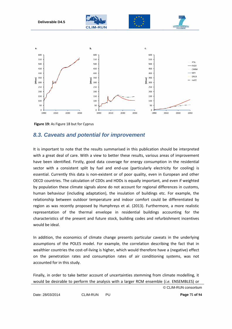
Deliverable D4.5



of 94

Figure 19: As Figure 18 but for Cyprus

8.3. Caveats and potential for improvement

It is important to note that the results summarised in this publication should be interpreted

with a great deal of care. With a view to better these results, various areas of improvement

have been identified. Firstly, good data coverage for energy consumption in the residential

sector with a consistent split by fuel and end-use (particularly electricity for cooling) is

essential. Currently this data is non-existent or of poor quality, even in European and other

OECD countries. The calculation of CDDs and HDDs is equally important, and even if weighted

by population these climate signals alone do not account for regional differences in customs,

human behaviour (including adaptation), the insulation of buildings etc. For example, the

relationship between outdoor temperature and indoor comfort could be differentiated by

region as was recently proposed by Humphreys et al. (2013). Furthermore, a more realistic

representation of the thermal envelope in residential buildings accounting for the

characteristics of the present and future stock, building codes and refurbishment incentives

would be ideal.

In addition, the economics of climate change presents particular caveats in the underlying

assumptions of the POLES model. For example, the correlation describing the fact that in

wealthier countries the cost-of-living is higher, which would therefore have a (negative) effect

on the penetration rates and consumption rates of air conditioning systems, was not

accounted for in this study.

Finally, in order to take better account of uncertainties stemming from climate modelling, it

would be desirable to perform the analysis with a larger RCM ensemble (i.e. ENSEMBLES) or

Deliverable D4.5



of 94

more recent climate model runs (i.e. the EURO-CORDEX/MED-CORDEX simulations).

Furthermore, since the CDD/HDD indices are calculated using fixed thresholds, the results are

highly susceptible to biases in the model simulations. A simple method of calibrating the

indices from model simulations to comparable indices from observed data (i.e., ensuring a

smooth transition between the past observed values and future simulate values) was used in

this study to help overcome this problem, but a more sophisticated method of first correcting

the raw temperature data also needs to be tested, and the effect on the results assessed. It

would also be useful to take into account other climate data besides average daily

temperature such as relative humidity for example, which is another key factor in human well-

being and therefore carries an important weight in the use of heating and cooling devices

along with the outdoor (dry bulb), surface temperature. The analysis presented here smooths

out year-to-year variability which may also be important for planning and management

purposes.

Deliverable D4.5



of 94

9. Closing Remarks

This report has provided a review of existing methodologies for assessing the socioeconomic

impacts of climate change and the potential benefits of adaptation. It has examined the

different ways in which climate change impacts have been assessed at different geographical

and sectoral resolutions, as well as reviewing the literature on the value of climate information

and climate services.

The main conclusion from this review is that there is some disconnect between the scientific

and high-level economic evidence of impacts (which is relatively abundant), and the relative

scarcity of studies demonstrating: i) how this evidence can be converted into meaningful

adaptation support for real-world actors; and ii) what the value of this type of information

would be.

On the one hand, the high-level studies described in Section 2 continue to take place alongside

studies that have a finer sectoral or geographical detail (such as those described Section 5 and

the case study sections 6-8). In addition, studies at all resolutions have begun to provide advice

on adaptation as well as impacts (Section 4).

On the other hand, very little peer-reviewed literature appears to exist concerning the ways in

which users in real life can make use of such information (i.e. the value of climate services).

Section 3 identified studies on the value of meteorological information in general, both in

terms of quantitative techniques and frameworks examining the usefulness of information to

different types of user. However, the review was unable to find any study that distinguished

climate services from other categories of meteorological information.

If climate services are to make a major contribution to improving people's adaptive capacity, it

is important to identify where such services can add value (in terms of improvements in

adaptive capacity and adaptation outcomes); which types of actors are capable of using them

(e.g. is the information usable by households and firms autonomously or does it require some

sort of collective or governmental action?); and therefore what form such services should take.

Deliverable D4.5



of 94

10. Glossary

During the drafting of this report, the authors have attempted to define key terms at the point where they first appear in the document. For any terms that are not explained adequately, we refer the reader to the glossaries provided by the Intergovernmental Panel on Climate Change (IPCC). http://www.ipcc.ch/publications_and_data/publications_and_data_glossary.shtml

http://www.ipcc.ch/publications_and_data/publications_and_data_glossary.shtml

Deliverable D4.5



of 94

11. References

Aaheim H A, Amundsen H, Dokken T & Wei T, 2012. Impacts and adaptation to climate change

in European economies, Global Environmental Change 22(4): 959–968.

Ackerman F., De Canio SJ., Howarth RB. & Sheeran K., 2009. Limitations of the integrated

assessment models of climate change. Climatic Change, 95, pp. 297–315.

Ackerman F & Munitz C, 2012. Climate damages in the FUND model: A disaggregated analysis.

Ecological Economics 77 219-224. doi:10.1016/j.ecolecon.2012.03.005

Agrawala S, Moehner A, El Raey M, Conway D, van Aalst M, Hagenstad M & Smith J, 2004.

Development and climate change in Egypt: Focus on Coastal Resources and the Nile,

OECD, Paris.

Agrawala, S. et al., 2010. Plan or React? Analysis of Adaptation Costs and Benefits Using

Integrated Assessment Models. OECD Environment Working Papers, No. 23, OECD

Publishing. http://dx.doi.org/10.1787/5km975m3d5hb-en

Ahmad Q K, Warrick R A, Downing T E, Nishioka S, Parikh K S, Parmesan C, Schneider S H, Toth

F & Yohe G, 2007. Methods and Tools. In: Climate change 2007 : impacts, adaptation

and vulnerability : contribution of Working Group II to the fourth assessment report of

the Intergovernmental Panel on Climate Change (J. J. McCarthy, O. F. Canziani, N. A.

Leary, D. J. Dokken and K. S. White, eds.), 105–143. Cambridge University Press,

Cambridge England.

http://www.grida.no/climate/ipcc_tar/wg2/pdf/wg2TARchap2.pdf.

Alexander, M.E., 2008. Proposed revision of fire danger class criteria for forest and rural areas

in New Zealand. Christchurch: National Rural Fire Authority, Wellington, in association

with the Scion Rural Fire Research Group.

Amelung B, Nicholls S & Viner D, 2007. Implications of Global Climate Change for Tourism Flows and Seasonality. Journal of Travel Research, 45, 285‐296.

Amelung B & Moreno A, 2009. Impacts of climate change in tourism in Europe: PESETA-

Tourism Study. JRC Scientific and Technical Reports, JRC IPTS

Anaman K A, Lellyett S C, Drake L, Leigh R J, Henderson-Sellers A, Noar P F, Sullivan P J,

Thampapillai D J, 1997. Benefits of meteorological services: evidence from recent

research in Australia, Meteorological Applications, 5, pp. 103–115.

Arrow K, 1965. Aspects of the Theory of Risk Bearing, Helsinki: Academic Publishers.

Artikov I, and Coauthors, 2006: Understanding the Influence of Climate Forecasts on Farmer

Decisions as Planned Behavior. Journal of Applied Meteorology & Climatology, 45,

1202–1214. doi: http://dx.doi.org/10.1175/JAM2415.1

ASHRAE, 2009. ASHRAE Handbook Fundamentals 2009, The American Society of Heating,

Refrigerating and Air-Conditioning Engineers, Inc., Atlanta, GA

http://dx.doi.org/10.1787/5km975m3d5hb-en

http://www.grida.no/climate/ipcc_tar/wg2/pdf/wg2TARchap2.pdf

http://dx.doi.org/10.1175/JAM2415.1

Deliverable D4.5



of 94

Balshi MS, McGuire AD, Duffy P, Flannigan M, Walsh J, Melillo J, 2009. Assessing the response

of area burned to changing climate in western boreal North America using a

Multivariate Adaptive Regression Splines (MARS) approach. Global Change Biology, 15,

578-600.

Bark R H, Colby B G & Dominguez F, 2010. Snow days? Snowmaking adaptation and the future

of low latitude, high elevation skiing in Arizona, USA.

Climatic Change, 102 3-4, pp 467-491

Barrio M, Loureiro M & Chas M C, 2007. Aproximación a las pérdidas económicas ocasionadas

a corto plazo por los incendios forestales en Galicia en 2006. Economía Agraria y

Recursos Naturales. ISSN: 1578-0732. Vol. 7, 14. pp. 45-64

Bassi S & Kettunen M, 2008. Forest Fires: causes and contributing factors in Europe. Report

prepared for European Parliament, Policy Department Economic & Scientific Policy.

IP/A/ENVI/ST/2007-15

Beaudoin Y & Pendleton L (eds.), 2012. Why Value the Oceans? A Discussion Paper. The

Economics of Ecosystems & Biodiversity

Beniston M, 2003. Climate change in mountain regions: A review of possible impacts. Climatic

Change, 59, 5‐31.

Biesbroek G, Swart R, Carter T, Cowan C, Henrichs T, Mela H, Morecroft M & Rey D, 2010.

Europe adapts to climate change: comparing national adaptation strategies. Global

Environmental Change 20 440-450. http://dx.doi.org/10.1016/j.gloenvcha.2010.03.005

Bigano A, Hamilton J M & Tol R S J, 2007a. The Impact of Climate Change on Domestic and

International Tourism: A Simulation Study, Integrated Assessment Journal, 7, 25-49.

Bigano A, Hamilton J & Tol R S J (2007b) “Nuove mete per il clima di domani”(New destinations

for tomorrow’s climate) La Rivista Del Turismo, Touring Club Italiano, Anno IX, N°3

Milano, Milan, Italy.

Bosello F. Adaptation, Mitigation and “Green” R&D to Combat Global Climate Change. Insights

From an Empirical Integrated Assessment Exercise. Centro Euro-Mediterraneo per i

Cambiamenti Climatici, Working Paper 20. Available from http://www.cmcc.it/wp-

content/uploads/2012/08/rp0048-cip-10-2008-1.pdf. Accessed 30/01/2014

Bosello F, Carraro C & De Cian E, 2009. An analysis of adaptation as a response to climate

change, Working Paper, Department of Economics, Ca'Foscari University of Venice No.

25/WP/2009.

Bosello F, Carraro C & de Cian E, 2011. Adaptation can Help Mitigation, an Integrated Approach

to post-2012 Climate Policy. Nota di Lavoro 69.2011. Fondazione Eni Enrico Mattei.

Bosello F, Eboli F & Pierfederici R, 2012. Assessing the economic impacts of climate change.

Review of Environment, Energy and Economics. FEEM.

Bosetti, V., C. Carraro, M. Galeotti, E. Massetti and M. Tavoni (2006), 'WITCH: A World Induced

Technical Change Hybrid Model', The Energy Journal, 27(Special Issue 2), 13-38

http://dx.doi.org/10.1016/j.gloenvcha.2010.03.005

http://www.cmcc.it/wp-content/uploads/2012/08/rp0048-cip-10-2008-1.pdf.%20Accessed%2030/01/2014

http://www.cmcc.it/wp-content/uploads/2012/08/rp0048-cip-10-2008-1.pdf.%20Accessed%2030/01/2014

Deliverable D4.5



of 94

Braathen N A, Lindhjem H & Navrud S, 2009. Valuing Lives Saved from Environmental,

Transport and Health Policies: A Meta-analysis of Stated Preference Studies.

Presentation to European Association of Environmental and Resource Economists, 17th

Annual Conference.

Brown S, Nicholls R, Vafeidis A, Hinkel J & Watkiss P, 2011. The Impacts and Economic Costs of

Sea level rise in Europe and the Costs and Benefits of Adaptation. Summary of Results

from the EC RTD ClimateCost Project. Technical Policy Briefing Note 2, The ClimateCost

Project. Stockholm Environment Institute, Stockholm, Sweden.

http://www.climatecost.cc/images/Policy_brief_2_Coastal_10_lowres.pdf.

Byram, G.M., 1959. Combustion of forest fuels. In K.P. Davis (Ed.), Forest Fire: Control and Use.

McGraw-Hill, New York, pp. 155-182.

Cai M, Ferrise R, Moriondo M, Nunes P & Bindi M, 2011. Climate Change and Tourism in

Tuscany, Italy. What if Heat becomes Unbearable? Fondazione Eni Enrico Mattei. Nota

di Lavoro 67.2011

Camia, A., Libertà, G., San-Miguel-Ayanz, J., 2012, Modelling impacts of climate change on

forest fire danger, PESETA II Forest Fires Study

Camia, A., Amatulli, G., 2009. Weather factors and fire danger in the Mediterranean, in: Earth

Observation of Wildland Fires in Mediterranean Ecosystems (E. Chuvieco, ed.),

Springer-Berlag, Berlin Heilderberg, pp. 71-82.

Camia, A., Durrant Houston, T., San-Miguel-Ayanz, J., 2010 The European Fire Database:

Development, Structure and Implementation. In: D.X. Viegas (Ed.) Proceedings VI

International Conference on Forest Fire Research, Coimbra, Portugal.

Cartalis C, Synodinou A, Proedrou M, Tsangrassoulis A, & Santamouris M, 2001. Modifications

in energy demand in urban areas as a result of climate changes: an assessment for the

southeast Mediterranean region. Energy Conversion and Management, vol. 42, no. 14,

pp. 1647-1656.

Carter T R, Jones R N, Lu X, Bhadwal S, Conde C, Mearns L O, O'Neill B C, Rounsvell M D A &

Zurek M B, 2007. New Assessment Methods and the Characterisation of Future

Conditions. Climate Change 2007: Impacts, Adaptation and Vulnerability. Contribution

of Working Group II to the Fourth Assessment Report of the Intergovernmental Panel

on Climate Change. Parry M L, Canziani O F, Palutikof J P, van der Linden P J, Hanson C

E, eds., Cambridge University Press, Cambridge, UK, 133-171.

Ceron J‐P & Dubois G (2005) The Potential Impacts of Climate Change on French Tourism.

Current Issues in Tourism, 8 (2), 125 ‐ 139.

Christensen J H, Hewitson B, Busuioc A, Chen A, Gao X, Held I, Jones R, Kolli R K, Kwon W T,

Laprise R, Magaña Rueda V, Mearns L, Menéndez C G, Räisänen J, Rinke A, Sarr A &

Whetton P, 2007. Regional Climate Projections. In: Climate Change 2007:The Physical

Science Basis. Contribution of Working Group I to the Fourth Assessment Report of the

http://www.climatecost.cc/images/Policy_brief_2_Coastal_10_lowres.pdf

Deliverable D4.5



of 94

Intergovernmental Panel on Climate Change. Solomon, S., D. Qin, M. Manning, Z. Chen,

M. Marquis, K.B. Averyt, M. Tignor and H.L. Miller (eds.). Cambridge University Press,

Cambridge, United Kingdom and New York, NY, USA.

Ciscar J-C, Saveyn B, van Regemorter D. Report on GEM-E3 modeling of climate impact.

Deliverable 6.1 of ClimateCost project.

Ciscar J-C. (editor), 2009. Climate Change impacts in Europe. Final Report of the PESETA

Project. JRC Scientific & Technical Reports, European Commission, Joint Research

Centre, Institute for Prospective Technological Studies. ISBN 978-92-79-14272-7.

doi:10.2791/32500

Ciscar J-C, Iglesias A, Feyen L, Szabó L, van Regemorter D, Amelung B, Nicholls R, Watkiss P,

Christensen O B, Dankers R, Garrote L, Goodess C M, Hunt A, Moreno A, Richards J &

Soria A, 2011. Physical and economic consequences of climate change in Europe. PNAS

108 (7) 2678-2683; doi:10.1073/pnas.1011612108

Ciscar J-C, Feyen L, Soria A, Lavalle C, Perry M, Raes F, Nemry F, Demirel H, Rozsai M, Dosio A,

DonatelliM, Srivastava A, Fumagalli D, Zucchini A, Shrestha S, Ciaian P, Himics M, Van

Doorslaer B, Barrios S, Ibáñez N, Rojas R, Bianchi A, Dowling P, Camia A, Libertà G, San

Miguel J, de Rigo D, Caudullo G, Barredo J-I, Paci D, Pycroft J, Saveyn B, Van

Regemorter D, Revesz T, Mubareka S, Baranzelli C, Rocha Gomes C, Lung T, Ibarreta D,

2013, Climate impacts in Europe: an integrated economic assessment (preliminary

results of the JRC PESETA II project), Impact World 2013, International Conference of

Climate Change Effects, Postdam, May 27-30.

Climate Change Impacts Study Committee, 2011. The Environmental, Economic and Social

Impacts of Climate Change in Greece. Bank of Greece, Athens. ISBN 978-960-7032-58-4

Cox P & Stephenson D, 2007. A Changing Climate for Prediction. Science 317(5835), 207–208.

doi:10.1126/science.1145956.

Croitoru L, 2007. How Much are Mediterranean Forests Worth? Forest Policy and Economics

Volume 9, Issue 5, January 2007, Pages 536–545

Dasgupta S, Laplante B, Murray S & Wheeler D, 2011. Exposure of developing countries to sea

level rise and storm surges. Climatic Change. Volume 106, Issue 4, pp 567-579

de Bruin KC., RB. Dellink, RSJ. Tol, 2009a. AD-DICE: An Implementation of Adaptation in the

DICE Model, Climatic Change, 95, pp. 63–81.

de Bruin, K. R. Dellink, and S. Agrawala, 2009b. Economic aspect of adaptation to climate

change: integrated assessment modelling of adaptation costs and benefits, OECD

Environment Working Paper no.6, March.

de Groot W. Interpreting the Canadian Forest Fire Weather Index (FWI) System.

http://www.dnr.state.mi.us/WWW/FMD/WEATHER/Reference/FWI_Background.pdf

Accessed 07/02/2014.

http://www.dnr.state.mi.us/WWW/FMD/WEATHER/Reference/FWI_Background.pdf

Deliverable D4.5



of 94

Dowling P, 2013. The impact of climate change on the European energy system. Energy Policy,

vol. 60, no. 0, pp. 406-417.

Dubois G, Alaouane T, Cauchy A, Ceron J P, Dubois C, Henia L, Hlaoui Z, Giannakopoulos C &

Zaninovic K, 2014. Reliability and usability of climate indices in the Mediterranean.

Deliverable from FP7 project CLIM-RUN (forthcoming)

Dumas P, Hallegatte S, Quintana-Segu P & Martin E, 2013. The influence of climate change on

flood risks in France – first estimates and uncertainty analysis. Nat. Hazards Earth Syst.

Sci., 13, 809–821. doi:10.5194/nhess-13-809-2013

Dumollard G & Leseur A, 2011. Drawing up a national climate change adaptation policy:

feedback from five European Case Studies. Climate Report No 27. CDC Climat Research

EEA (European Environmental Agency), 2012. Climate change, impacts and vulnerability in

Europe 2012, An indicator-based report, ISSN 1725-9177

EURAC, 2007. Impacts of Climate Change on winter tourism in the Italian Alps. ClimChalp

INTERREG III B Alpine Space Project Report.

Fankhauser S, 2010. The cost of adaptation, Climate Change, 1(1), pp. 23-30.

Feyen L & Watkiss P, 2011. Technical Policy Briefing Note 3. The Impacts and Economic Costs

of River Floods in Europe, and the Costs and Benefits of Adaptation. Results from the

EC RTD ClimateCost Project. In Watkiss, P (Editor), 2011. The ClimateCost Project. Final

Report. Published by the Stockholm Environment Institute, Sweden, 2011. ISBN. 978-

91-86125-35-6.

Feyen L, Dankers R, Bódis K, Salamon P. & Barredo J I, 2011. Fluvial flood risk in Europe in

present and future climates. Climatic Change 112(1), 47–62. doi:10.1007/s10584-011-

0339-7.

Fitzgerald J & Lindner M (eds.), 2013. Adapting to climate change in European forests - Results

of the MOTIVE project. Pensoft Publishers, Sofia, 108 pp.

Flannigan, M. D., Stocks, B. J., Wotton, B. M., 2000. Climate Change and Forest Fires, The

Science of the Total Environment 262:221-229.

Flannigan M D, Krawchuk M A, de Groot W J, Wotton B M & Gowman L M, 2009. Implications

of changing climate for global wildland fire. International Journal of Wildland Fire 18,

483–507. http://dx.doi.org/10.1071/WF08187

FWI (Finnish Meteorological Institute), 2012. Economic value of weather forecasts on

transportation – Impacts of weather forecast quality developments to the economic

effects of severe weather. Deliverable 5.2 of project EWENT (Extreme Weather

impacts on European Networks of Transport). http://ewent.vtt.fi

Frei T, von Grünigen S & Willemse S, 2012. Economic benefit of meteorology in the Swiss road

transportation sector. Meteorological Applications published online, 01/06/2012. DOI:

10.1002/met.1329

Friedman JH, 1991, Multivariate adaptive regression splines. The Annals of Statistics, 19, 1-141.

http://ewent.vtt.fi/

Deliverable D4.5



of 94

Fuchs S, Birkmann J & Glade T, 2012. Vulnerability assessment in natural hazard and risk

analysis: current approaches and future challenges. Natural Hazards, Volume 64, Issue

3, pp 1969-1975

Gaudard L & Romerio F, 2013. The future of hydropower in Europe: Interconnecting climate,

markets and policies. Environmental Science & Policy. Available online 2 November

2013.In Press, Corrected Proof. http://dx.doi.org/10.1016/j.envsci.2013.09.008

Giannakopoulos C, Le Sager P, Bindi M, Moriondo M, Kostopoulou E, Goodess CM (2009),

Climatic change and associated impacts in the Mediterranean resulting from a 2°C

global warming. Global Planet Change, 68:209–224

Goodess C.M., C. Hanson M. Hulme & T.J. Osborn, 2003: Representing climate and extreme

weather events in integrated assessment models: a review of existing methods and

options for development. Integrated Assess. J., 4, 145-171.

Grothmann T & Patt A, 2005. Adaptive capacity and human cognition: The process of individual

adaptation to climate change. Global Environmental Change. Volume 15, Issue 3,

October 2005, Pages 199–213

Gualdi, S., Somot, S., Li, L., Artale, V., Adani, M., Bellucci, A., Braun, A., Calmanti, S., Carillo, A.,

Dell'Aquila, A., Déqué, M., Dubois, C., Elizalde, A., Harzallah, A., Jacob, D., L'Hévéder,

B., May, W., Oddo, P., Ruti, P., Sanna, A., Sannino, G., Scoccimarro, E., Sevault, F. and

Navarra, A., 2013. The CIRCE Simulations: Regional Climate Change Projections with

Realistic Representation of the Mediterranean Sea. Bulletin of the American

Meteorological Society, vol. 94, no. 1, pp. 65-81.

Hallegatte S and co-authors, 2008. Assessing Climate Change Impacts, Sea Level Rise and

Storm Surge Risk in Port Cities, OECD Environment Working Papers No 3, OECD

Publishing, Paris.

Hallegatte S, Ranger N, Mestre O, Dumas P, Corfee-Morlot J, Herweijer C & Muir Wood R,

2011. Assessing climate change impacts, sea level rise and storm surge risk in port

cities: a case study on Copenhagen. Climatic Change, Volume 104, Issue 1, pp 113-137

Hallegatte S, Green C, Nicholls R J & Corfee-Morlot J, 2013. Nature Climate Change 3, 802–806.

doi:10.1038/nclimate1979

Hamilton J M & Tol R S J, 2007. The impact of climate change on tourism in Germany, the UK

and Ireland: a simulation study. Regional Environmental Change 7: 161-172.

http://www.fnu.zmaw.de/fileadmin/fnu-files/publication/working-

papers/regtourwp.pdf.

Hamilton J M, Maddison D J & Tol R S J (2005a) Climate change and international tourism: a

simulation study. Global Environmental Change Part A, 15(3), 253-266.

Hanson S, Nicholls R, Ranger N, Hallegatte S, Corfee-Morlot J, Herweijer C & Chateau J, 2011. A

global ranking of port cities with high exposure to climate extremes. Climatic Change,

Volume 104, Issue 1, pp 89-111.

http://dx.doi.org/10.1016/j.envsci.2013.09.008

Deliverable D4.5



of 94

Hardee K & Mutunga C 2010. Strengthening the link between climate change adaptation and

national development plans: lessons from the case of population in National

Adaptation Programmes of Action (NAPAs). Mitigation and Adaptation Strategies for

Global Change, 15:113-126.

Hawkins E & Sutton R, 2009. The Potential to Narrow Uncertainty in Regional Climate

Predictions. Bulletin of the American Meteorological Society 90(8), 1095–1107.

doi:10.1175/2009BAMS2607.1.

Hekkenberg M, Moll H C & Uiterkamp A J M S, 2009. Dynamic temperature dependence

patterns in future energy demand models in the context of climate change. Energy,

vol. 34, no. 11, pp. 1797-1806.

Heltberg R, Siegel P B & Jorgensen S L, 2009. Addressing human vulnerability to climate

change: Toward a ‘no-regrets’ approach. Global Environmental Change Volume 19,

Issue 1, pp. 89–99

Hinkel J & Klein R J T,2009. Integrating knowledge to assess coastal vulnerability to sea level

rise: The development of the DIVA tool. Global Environmental Change 19.3, pp. 384–

395. doi: 10.1016/j.gloenvcha. 2009.03.002.

Hinkel J, Nicholls R J, Vafeidis A, Tol R S J & Avagianou T, 2010. Assessing risk of and adaptation

to sea level rise in the European Union: an application of DIVA. Mitigation and

Adaptation Strategies for Global Change 5.7, pp. 1–17. doi: 10.1007/s11027-010-9237-

y.

Holman I.P., Rounsevell M.D.A., Shackley S., Harrison P.A., Nicholls R.J., Berry P.M. and Audsley

E., 2005. A regional, multi-sectoral and integrated assessment of the impacts of

climate and socioeconomic change in the UK: I Methodology. Climatic Change, 71, 9-

41.

Holman, I.P. Nicholls, R.J. Berry, P.M. Harrison, P.A. Audsley, E. Shackley, S. and Rounsevell,

M.D.A., 2005a. A regional, multi-sectoral and integrated assessment of the impacts of

climate and socioeconomic change in the UK: II Results. Climatic Change, 71, 43-73.

Hooke W H, Pielke Jr R A, 2000. Short-term weather prediction: an orchestra in search of a

conductor, in D. Sarewitz, RA. Pielke, Jr., and R. Byerly (eds), Prediction: Decision

Making and the Future of Nature, Chapter 5, Island Press: Washington, DC

Hope C W, 2006. The marginal impact of CO2 from PAGE2002: an integrated assessment model incorporating the IPCC’s five reasons for concern, Integrated Assessment Journal, 6(1), pp. 19–56

Hope, C. and Newbery, D., 2007. Calculating the social cost of carbon. Electricity Policy Research Group Working Papers, No.EPRG 07/20. Cambridge: University of Cambridge.

Hope CW., J. Anderson, P. Wenman (1993), Policy Analysis of the Greenhouse effect: an Application of the PAGE model, Energy Policy, 21(3), pp. 327-338.

Hu Q and Coauthors, 2006: Understanding Farmers’ Forecast Use from Their Beliefs, Values, Social Norms, and Perceived Obstacles. Journal of Applied Meteorology & Climatology, 45, 1190–1201. doi: http://dx.doi.org/10.1175/JAM2414.1

http://dx.doi.org/10.1175/JAM2414.1

Deliverable D4.5



of 94

Humphreys M A , Rijal H B & Nicol J F, 2013. Updating the adaptive relation between climate and comfort indoors; new insights and an extended database. Building and Environment, vol. 63, no. 0, pp. 40-55.

Hunt A, Watkiss P, 2007. Literature review on climate change impacts on urban cities centres. Initial findings, Paris, OECD Publications.

Hutton G, 2009 Concept Note – Protecting Health from Global Climate Change: Proposals for using Economic Analysis to Enhance Policy & Decision Support to Member States http://www.adaptationlearning.net/system/files/CN%20on%20Health%20Economics%20and%20Climate%20Change%20Adaptation%2C%20WHO.pdf

Iglesias A., Quiroga S. and Garrote L, 2010, Work Package 2B Agriculture and Water, Deliverable D2B, ClimateCost project

IMAGE Team, 2001. The IMAGE 2.2 Implementation of the SRES Scenarios: A Comprehensive Analysis of Emissions, Climate Change and Impacts in the 21st Century [CD-ROM] RIVM CD-ROM Publication 481508018. Bilthoven: National Institute for Public Health and the Environment.

Interagency Working Group on the Social Cost of Carbon, 2013. Technical Support Document. Technical Update of the Social Cost of Carbon for Regulatory Impact Analysis – Under Executive Order 12866. Available from http://www.whitehouse.gov/sites/default/files/omb/inforeg/social_cost_of_carbon_for_ria_2013_update.pdf. Accessed 29/01/2014.

IPCC, 2001: Climate Change 2001: Synthesis Report. A Contribution of Working Groups I, II, and III to the Third Assessment Report of the Integovernmental Panel on Climate Change [Watson, R.T. and the Core Writing Team (eds.)]. Cambridge University Press, Cambridge, United Kingdom, and New York, NY, USA, 398 pp.

IPCC, 2007: Climate Change 2007: Synthesis Report. Contribution of Working Groups I, II and III to the Fourth Assessment Report of the Intergovernmental Panel on Climate Change [Core Writing Team, Pachauri, R.K and Reisinger, A. (eds.)]. IPCC, Geneva, Switzerland, 104 pp.

IPCC, 2012: Managing the Risks of Extreme Events and Disasters to Advance Climate Change Adaptation. A Special Report of Working Groups I and II of the Intergovernmental Panel on Climate Change [Field, C.B., V. Barros, T.F. Stocker, D. Qin, D.J. Dokken, K.L. Ebi, M.D. Mastrandrea, K.J. Mach, G.-K. Plattner, S.K. Allen, M. Tignor, and P.M. Midgley (eds.)]. Cambridge University Press, Cambridge, UK, and New York, NY, USA, 582 pp.

IPCC, 2013: Climate Change 2013: The Physical Science Basis. Contribution of Working Group I to the Fifth Assessment Report of the Intergovernmental Panel on Climate Change [Stocker, T.F., D. Qin, G.-K. Plattner, M. Tignor, S.K. Allen, J. Boschung, A. Nauels, Y. Xia, V. Bex and P.M. Midgley (eds.)]. Cambridge University Press, Cambridge, United Kingdom and New York, NY, USA, 1535 pp.

Isaac M & van Vuuren D P, 2009. Modeling global residential sector energy demand for heating and air conditioning in the context of climate change. Energy Policy 37 (2009) 507–521

Isoard S, Watkiss P, Voigt T, Barredo J, Kristensen P, Menne B, 2008. Chapter7.9: Tourism and recreation. In: Saunders, P., Ullstein, B., Swart, R.(Eds.), Impact of Europe’s changing climate, 2008 indicator-°C‐based assessment. EEAReport No4/2008.European Communities Copenhagen pp187–189,

http://www.adaptationlearning.net/system/files/CN%20on%20Health%20Economics%20and%20Climate%20Change%20Adaptation%2C%20WHO.pdf

http://www.adaptationlearning.net/system/files/CN%20on%20Health%20Economics%20and%20Climate%20Change%20Adaptation%2C%20WHO.pdf

http://www.whitehouse.gov/sites/default/files/omb/inforeg/social_cost_of_carbon_for_ria_2013_update.pdf

http://www.whitehouse.gov/sites/default/files/omb/inforeg/social_cost_of_carbon_for_ria_2013_update.pdf

Deliverable D4.5



of 94

Jones B & Scott D, 2006. Implications of Climate change for visitation to Ontario’s provincial parks. Leisure, 30 (1), 233‐262.

JRC (Joint Research Centre), 2011. Forest Fires in Europe 2010. JRC Scientfic and Technical Reports. Report No. 11. EUR 24910 EN - 2011

Katz R W & Murphy A H, 1997. Economic value of weather and climate forecasts, Cambridge, Cambridge University Press.

Katz, R. et al., 2013 Uncertainty analysis in climate change assessments. Nature Climate Change 3, 769-771 .

Kent M, Newham R & Essex S, 2002. Tourism and sustainable water supply in Mallorca: a geographical analysis. Applied Geography, 22(4), 351‐374.

Klein D R, Olonscheck M, Walther C & Kropp J, 2013. Susceptibility of the European electricity sector to climate change, Energy, vol. 59, no. 0, pp. 183-193.

Knight F H, 1921. Risk, uncertainty and profit, Boston printing Klockow K E, McPherson R A & Sutter D S, 2010. On the Economic Nature of Crop Production

Decisions Using the Oklahoma Mesonet. Weather, Climate, and Society, 2, 224–236. doi: http://dx.doi.org/10.1175/2010WCAS1034.1

Kolström M, Vilén T & Lindner M, 2011. Climate Change Impacts and Adaptation in European Forests. EFI Policy Brief 6 http://www.efi.int/files/attachments/publications/efi_policy_brief_6_eng_net.pdf

Kovats R S, Lloyd S, Hunt A & Watkiss P, 2011. The Impacts and Economic Costs on Health in Europe and the Costs and Benefits of Adaptation. Results of the EC RTD ClimateCost Project. In: The ClimateCost Project. Final Report. Volume 1: Europe (P. Watkiss, ed.). Stockholm Environment Institute, Sweden. http://www.climatecost.cc/reportsandpublications.html.

Kundzewicz Z W, Lugeri N, Dankers R, Hirabayashi Y, Döll P, Pińskar I, Dysarz T, Hochrainer S & Matczak P, 2010. Assessing river flood risk and adaptation in Europe—review of projections for the future. Mitig Adapt Strateg Glob Change 15:641–656 doi 10.1007/s11027-010-9213-6

Landau S, 2010. Socio-economic assessments of climate change impacts: A stock-taking report. Prepared for: The United Nations Development Programme – Bratislava Regional Centre by Seth Landau, Eco Ltd.

Lazo J K & Chestnut L G, 2002. Economic Value of Current and Improved Weather Forecasts in the US Household Sector. Report prepared for Dr. Rodney Weiher, Chief Economist, Office of Policy and Strategic Planning by Stratus Consulting with the financial support of the NPOESS, National Environmental Satellite Data and Information Service National Oceanic and Atmospheric Administration.

Lehner B, Czisch G & Vassolo S, 2005. The impact of global change on the hydropower

potential of Europe: a model-based analysis. Energy Policy. Volume 33, Issue 7, May

2005, Pages 839–855. http://dx.doi.org/10.1016/j.enpol.2003.10.018

Leone, V., Lovreglio, L., Pilar Martín, M., Martínez, J., & Vilar, L. (2009). Chapter 11 human

factors of fire occurrence in the Mediter- ranean. In E. Chuvieco (Ed.), Earth

observation of wildland fires in Mediterranean ecosystems (pp. 149-170). Berlin,

Heidelberg: Springer-Verlag.

http://dx.doi.org/10.1175/2010WCAS1034.1

http://www.efi.int/files/attachments/publications/efi_policy_brief_6_eng_net.pdf

http://www.climatecost.cc/reportsandpublications.html

http://dx.doi.org/10.1016/j.enpol.2003.10.018

Deliverable D4.5



of 94

Malone, E.L. & La Rovere E;L., 2005. Assessing current and changing socioeconomic conditions.

In Adaptation Policy Frameworks for Climate Change: Developing Strategies,

Strategies, Policies and Measures, B. Lim, E. Spanger-Siegfried, I. Burton, E.Malone and

S. Huq, Eds., CambridgeUniversity Press, Cambridge and New York, 145-163.

Markandya A & Chiabai A, 2009. Valuing Climate Change Impacts on Human Health: Empirical

Evidence from the Literature. Int J Environ Res Public Health. February; 6(2): 759–786.

Published online 2009 February 23. doi: 10.3390/ijerph6020759

Mavsar R., Pettenella D., San-Miguel J., Camia A., 2011. Development of a methodology for the

analysis of socio-economic impact of forest fires in Europe. In: Proc. 5th International

Wildfire Conference, Sun City, South Africa, 9-13 May 2011.

McNeil M & Letschert V E, 2007. Future air conditioning energy consumption in developing

countries and what can be done about it: the potential of efficiency in the residential

sector. ECEEE 2007 Summer Study, pp. 1311-1322

Merrill, D. F., Alexander, M. E., 1987. Glossary of forest fire management terms, National

Research Council of Canada, Canadian Committee on Forest Fire Management,

Ottawa, Ontario.

Mieczkowski Z, 1985. The tourism climatic index: A method of evaluating world climates for

tourism. Canadian Geographer, 29(3), 220-233.

Mima S & Criqui P, 2009. Assessment of the impacts under future climate change on the

energy systems with the POLES model, International energy workshop Venice: Italy

(2009), Fondazione Giorgio Cini,Venice, Italy

Moss R H, Edmonds J A, Hibbard K A, Manning M R, Rose S K, van Vuuren D P, Carter T R, Emori

S, Kainuma M, Kram T, Meehl G A, Mitchell J F B, Nakicenovic N, Riahi K, Smith S J,

Stouffer R J, Thomson A M, Weyant J P & Wilbanks T J., 2010. The next generation of

scenarios for climate change research and assessment. Nature 463, 747-756.

doi:10.1038/nature08823

Nakicenovic, N. & Swart, R. (eds.) (2000) Special Report on Emissions Scenarios. Cambridge

University Press, Cambridge, United Kingdom.

Natural Resources Canada, 2008. Canadian Wildland Fire Information System. Extract from

web page, accessed 07/02/2014.

http://cwfis.cfs.nrcan.gc.ca/background/summary/FWI

Nickerson N, Becerra L & Zumstein P, 2011. Climate Change & Tourism Literature Review.

Institute for Tourism & Recreation Research, University of Montana. Research Report

2011-1.

Nicholls S, 2006. Climate change, tourism and outdoor recreation in Europe. Managing Leisure,

11 (3) 151‐163.

Nicholls R J, Wong P P, Burkett V R, Codignotto J O, Hay J E, McLean R F, Ragoonaden S &

Woodroofe C D, 2007. Coastal systems and low-lying areas. Climate Change 2007:

http://cwfis.cfs.nrcan.gc.ca/background/summary/fwi

Deliverable D4.5



of 94

Impacts, Adaptation and Vulnerability. Contribution of Working Group II to the Fourth

Assessment Report of the Intergovernmental Panel on Climate Change, M.L. Parry,

O.F. Canziani, J.P. Palutikof, P.J. van der Linden and C.E. Hanson, Eds., Cambridge

University Press, Cambridge, UK, 315-356.

Nicholls R, 2007. Adaptation Options for Coastal Areas and Infrastructure: an Analysis for 2030.

Technical Report UNFCCC, Bonn, Germany.

Nicholls R, Brown S, Hanson S & Hinkel J, 2010. Economics of Coastal Zone Adaptation to

Climate Change. World Bank Discussion Paper Number 10.

Njie M, 2008. Costing Priority Adaptations: A View from NAPAs, paper presented at the OECD

Workshop on Economic Aspects of Adaptation to Climate Change, Paris, 7-8 April.

Nordhaus W D, and Boyer J G, 2000. Warming the World: Economic Models of Global

Warming, Cambridge: The MIT Press.

Nordhaus W D., 2010. Economic aspects of global warming in a post-Copenhagen

environment. PNAS. 107 (26) 11721-11726; published ahead of print June 14, 2010,

doi:10.1073/pnas.1005985107

OECD, 2008. Economic Aspects of Adaptation to Climate Change: Costs, Benefits and Policy

Instruments. Organisation for Economic Cooperation and Development (OECD). ISBN-

978-92-64-04603-0

OECD, 2012. Farmer Behaviour, Agricultural Management and Climate Change, OECD

Publishing. http://dx.doi.org/10.1787/9789264167650-en

Oehler F, Oliveira S, Barredo JI, Camia A, San Miguel Ayanz J, Pettenella D, Mavsar R, 2012.

Assessing European Wildfire Vulnerability. Geophysical Research Abstracts, Vol. 14,

EGU2012-9452, EGU General Assembly 2012.

Olesen J E, Carter T R, Díaz-Ambrona C H, Fronzek S, Heidmann T, Hickler T, Holt T, Minguez M

I, Morales P, Palutikof J P, Quemada M, Ruiz-Ramos M, Rubæk G H, Sau F, Smith B et

al., 2007. Uncertainties in projected impacts of climate change on European

agriculture and terrestrial ecosystems based on scenarios from regional climate

models. Climatic Change 81, 123–143. doi:10.1007/s10584-006-9216-1.

O’Neill B.C., Carter T.R., Ebi K.L., Edmonds J., Hallegatte S., Kemp-Benedict E., Kriegler E.,

Mearns L., Moss R., Riahi K., van Ruijven B., van Vuuren D. 2012. Meeting Report of the

Workshop on The Nature and Use of New Socioeconomic Pathways for Climate Change

Research, Boulder, CO, November 2-4, 2011. Available at:

http://www.isp.ucar.edu/socio-economic-pathways.

Parry M, Arnell N, Berry P, Dodman D, Fankhauser S, Hope C, Kovats S, Nicholls R,

Satterthwaite D, Tiffin R, Wheeler T, 2009. Assessing the Costs of Adaptation to

Climate Change: A Review of the UNFCCC and Other Recent Estimates. International

Institute for Environment and Development and Grantham Institute for Climate

Change, London.

http://www.isp.ucar.edu/socio-economic-pathways

Deliverable D4.5



of 94

Patt A, Suarez P & Gwata C, 2005. Effects of seasonal climate forecasts and participatory

workshops among subsistence farmers in Zimbabwe, PNAS, Vol. 102, No.12, pp.

12623–12628.

Patt AG., DP. van Vuuren, F. Berkhout, A. Aaheim, AF. Hof, M. Isaac and R. Mechler, 2010.

Adaptation in integrated assessment modeling: where do we stand?, Climatic Change,

99(3-4), pp. 383-402.

Peltonen L, Sikku J & Schuster P. Governance of Climate Change Adaptation: Policy Review.

Report for BaltCICA project. http://www.baltcica.org/results/documents.html

Perrels A, Nurmi V & Nurmi P, 2012. Weather service chain analysis (WSCA) – An approach for

appraisal of the social-economic benefits of improvements in weather services,

SIRWEC Conference, Helsinki, 23–25 May 2012, paper 0081,

http://www.sirwec2012.fi/Extended Abstracts/002 Perrels.pdf, 2012.

Perry M & Ciscar J-C, 2014. Multisectoral Perspective in Modelling of Climate Impacts and

Adaptation. Chapter in Routledge Handbook on Economics of Adaptation to Climate

Change. Eds. Markandya A, Gallaraga I & Sainz de Murieta E. Routledge, 2014. ISBN-

978-0-415-63311-6.

Piontek F, Pugh T A M, Clark D B, Deryng D, Elliott J, de Jesus Colón González F, Flörke M,

Folberth C, Franssen W, Frieler K, Friend A D, Gosling S N, Hemming D, Khabarov N,

Kim H, Lomas M R, Masaki Y, Mengel M, Morse A, Neumann K, Nishina K, Ostberg S,

Pavlick R, Ruane A C, Schewe J, Schmid E, Stacke T, Tang Q, Tessler Z D, Tompkins A M,

Warszawski L, Wisser D & Schellnhuber H J, 2013. Multisectoral climate impact

hotspots in a warming world. PNAS, published ahead of print December 16, 2013,

doi:10.1073/pnas.1222471110

Plan Bleu: Adapting to climate change in water sector in the Mediterranean: situation and

prospects, 2011. Plan Bleu, Valbonne (Blue Plan Papers 10).

Pratt J, 1964. Risk aversion in the small and in the large. Econometrica 32, pp.122–136.

Ramos M H, van Andel S J & Pappenberger F, 2013. Do probabilistic forecasts lead to better

decisions? Hydrology and Earth System Sciences, 17, 2219–2232.

doi:10.5194/hess-17-2219-2013

Ranger N & coauthors, 2011. An assessment of the potential impact of climate change on flood

risk in Mumbai. Climatic Change, January 2011, Volume 104, Issue 1, pp 139-167.

Richards J & Nicholls RJ, 2009. Impacts of climate change in coastal systems in Europe. PESETA

Coastal Systems study. JRC Scientific and Technical Reports, EUR 24130.

Riera P & Mogas J, 2004. Evaluation of a risk reduction in forest fires in a Mediterranean

region. Forest Policy and Economics. Volume 6, Issue 6, October 2004, Pages 521–528

Rojas R, Feyen L & Watkiss P, 2013. Climate change and river floods in the European Union:

Socio-economic consequences and the costs and benefits of adaptation. Global

Environmental Change. Volume 23, Issue 6, Pages 1737–1751

http://www.baltcica.org/results/documents.html

Deliverable D4.5



of 94

Román M V, Azqueta D, Rodrígues M, 2013. Methodological approach to assess the socio-

economic vulnerability to wildfires in Spain. Forest Ecology and Management. Volume

294, 15 April 2013, Pages 158–165

San-Miguel-Ayanz, J., Carlson, J. D., Alexander, M., Tolhurst, K., Morgan, G., Sneeuwjagt, R.,

Dudley, M., 2003. Current methods to assess fire danger potential, in: Wildland fire

danger estimation and mapping - The Role of Remote Sensing Data (E. Chuvieco, ed.),

World Scientific Publishing, Singapore, pp. 22-61.

San-Miguel-Ayanz, J., Moreno J.M., Camia A., 2012. Analysis of large fires in European

Mediterranean landscapes: Lessons learnt and perspectives. Forest Ecology and

Management. Manuscript accepted for publication.

Santos F D, Stigter T Y, Faysse N & Lourenço T C, 2014. Impacts and adaptation to climate

change in the Mediterranean coastal areas: the CIRCLE-MED initiative. Regional

Environmental Change, Volume 14, Issue 1 Supplement, pp 1-3

Ščasný M & Alberini A, 2012. Valuation of Mortality Risk Attributable to Climate Change:

Investigating the Effect of Survey Administration Modes on a VSL. Int J Environ Res

Public Health. 2012 December; 9(12): 4760–4781. Published online 2012 December 18.

doi: 10.3390/ijerph9124760

Schlesinger ME & Williams L J, 1998. COSMIC 1.1 Country-Specific Model for Intertemporal

Climate. Palo Alto: Electric Power Research Institute.

Scott D, Wall G & McBoyle G, 2005. The Evolution of the Climate Change Issue in the Tourism

Sector. In: J E S Higham (ed.), Tourism, Recreation and Climate Change, Chapter 3, pp.

44-60.

Scott D, Gössling S & Hall C, 2012. International Tourism and Climate Change. WIREs Clim

Change, 3:213-232. doi:10.1002/wcc.165

SEI (Stockholm Environment Institute), 2010. AdaptCost Briefing Paper 1: Integrated

Assessment Models – Africa results.

Sharma U & Patt A, 2012. Disaster warning response: the effects of different types of personal

experience, Natural Hazards, Vol.60, pp. 409-423.Stern N, 2007. The Economics of

Climate Change, the Stern Review. Cambridge UniversityPress, ISBN 9780521700801.

Stocks, B.J., Lawson, B.D., Alexander, M.E., Van Wagner, C.E., McAlpine, R.S., Lynham, T.J.

Dubé D.E., 1989. The Canadian Forest Fire Danger Rating System: An overview. The

Forestry Chronicle 65, 258-265.

Sullivan P, 2013. NREL/CFDDA Global Wind Supply curves. 2013 CCI/IA Workshop, July 22,

2013. http://emf.stanford.edu/files/docs/340/Patrick_Sullivan_7.22_AM.1.pdf

Swart R, Biesbroek R, Binnerup S, Carter T R, Cowan C, Henrichs T, Loquen S, Mela H,

Morecroft M, Reese M & Rey D, 2009. Europe Adapts to Climate Change: Comparing

National Adaptation Strategies. PEER Report No 1. Helsinki: Partnership for European

Environmental Research.

http://emf.stanford.edu/files/docs/340/Patrick_Sullivan_7.22_AM.1.pdf

Deliverable D4.5



of 94

TEEB ,2010. Mainstreaming the economics of nature: A synthesis of the approach, conclusions

and recommendations of TEEB. The Economics of Ecosystems and Biodiversity.

http://us-

cdn.creamermedia.co.za/assets/articles/attachments/30310_teeb_synthreport_09_20

10_online.pdf.

TEEB, 2012. The Economics of Ecosystems and Biodiversity in Local and Regional Policy and

Management. Edited by Heidi Wittmer and Haripriya Gundimeda. Earthscan, London

and Washington.

Teisberg T J & Weiher R F, 2009. Benefits and costs of early warning systems for major natural

hazards. Background paper, World Bank Group

Tol R S J, 1999. Spatial and temporal efficiency in climate policy: applications of FUND.

Environmental and Resource Economics, 14(1), 33-49.

Tol R S J, 2002. New estimates of the damage costs of climate change, Part I: Benchmark

estimates. Environmental and Resource Economics 21 (1): 47-73.

UKCIP, 2004. Costing the impact of climate change in UK. Implementation report. Final report

UNISDR (United Nations International Strategy for Disaster Risk Reduction), EUR-OPA (Major

Hazards Agreement) & CoE (Council of Europe), 2011. Climate Change Adaptation and

Disaster Risk Reduction in Europe: a Review of Risk Governance.

http://preventionweb.net/go/20591

UNFCCC, 2007. Investment and Financial Flows to Address Climate Change. UNFCCC

Secretariat, ISBN 92-9219-042-3

Van der Ploeg, S. & R.S. de Groot, 2010. The TEEB Valuation Database – a searchable database

of 1310 estimates of monetary values of ecosystem services. Foundation for

Sustainable Development, Wageningen, The Netherlands. http://www.es-

partnership.org/esp/80763/5/0/50

Van der Linden, P. and Mitchell, J.F.B. (Eds.), 2009. ENSEMBLES: climate change and its

impacts: Summary of research and results from the ENSEMBLES project, Met Office

Hadley Centre, FitzRoy Road, Exeter EX1 3PB, UK. 160pp.

Van Vliet M T H, Yearsley J R, Ludwig F, Vogele S, Lettenmaier D P & Kabat P, 2012.

Vulnerability of US and European electricity supply to climate change, Nature Clim.

Change, vol. 2, no. 9, pp. 67

van Vuuren D., Edmonds J., Kainuma M., Riahi K. and Weyant J, 2011. A special issue on the

RCPs. Climatic Change 109(1), 1–4. doi:10.1007/s10584-011-0157-y.

Van Wagner, C. E., 1987. Development and structure of the Canadian Forest Fire Weather

Index System, Canadian Forestry Service, Ottawa, Ontario, pp. 37.

Varela E, Giergiczny M, Riera P, Mahieu P A, Soliño M, 2012. Economic valuation of forest fire

programs in Andalusia (Spain): Social preferences and willingness to pay. 14th Annual

http://us-cdn.creamermedia.co.za/assets/articles/attachments/30310_teeb_synthreport_09_2010_online.pdf



http://preventionweb.net/go/20591

Deliverable D4.5



of 94

Bioecon Conference on “Resource Economics, Biodiversity Conservation and

Development” 18‐20 September 2012. Kings College, Cambridge United Kingdom

Watkiss P., Downing T., 2008, The Social Cost of Carbon: Valuation Estimates and Their Use in

UK Policy, Integrated Assessment Journal. Vol. 8, Iss. 1, pp. 85–105.

Watkiss, P., Downing, T., Dyszynski, J.: 2010 AdaptCost Project: Briefing Paper 1: Integrated

Assessment Models – Africa results. UNEP, Nairobi.

Weaver C P, Lempert R J, Brown C, Hall J A, Revell D & Sarewitz D, 2013. Improving the

contribution of climate model information to decision making: the value and demands

of robust decision frameworks. WIREs Clim Change, 4:39–60. doi: 10.1002/wcc.202

Wilby R L, Charles S P, Zorita E, Timbal B, Whetton P & Mearns L O, 2004. Guidelines for Use of

Climate Scenarios Developed from Statistical Downscaling Methods. IPCC Task Group

on Data and Scenario Support for Impact and Climate Analysis (TGICA).

Wilby, R. L., Charles, S. P., Zorita, E., Timbal, B., Whetton, P. & Mearns, L. O., 2004. Guidelines

for Use of Climate Scenarios Developed from Statistical Downscaling Methods. IPCC

Task Group on Data and Scenario Support for Impact and Climate Analysis (TGICA),

http://ipcc-ddc.cru.uea.ac.uk/guidelines/StatDown_Guide.pdf

Wilby, R. L., Beven, K. J. and Reynard, N. S. (2008), Climate change and fluvial flood risk in the

UK: more of the same?. Hydrol. Process., 22: 2511–2523. doi: 10.1002/hyp.6847

Wilks D S, 2001. A skill score based on economic value for probability forecasts. Meteorological

Applications, vol.8, pp. 209–219.

WMO (World Meteorological Association), 2011. Climate Knowledge for Action: a Global

Framework for Climate Services — Empowering the Most Vulnerable. The Report of

the High-Level Task Force for the Global Framework for Climate Services. WMO-No.

1065.

World Bank. 2010. Economics of adaptation to climate change - Synthesis report. Washington,

DC: World Bank.

Yip S, Ferro C A T, Stephenson D B & Hawkins E, 2011. A Simple, Coherent Framework for

Partitioning Uncertainty in Climate Predictions. Journal of Climate 24(17), 4 634–4 643.

doi:10.1175/2011JCLI4085.1.

Yohe, G.W., R.D. Lasco, Q.K. Ahmad, N.W. Arnell, S.J. Cohen, C. Hope, A.C. Janetos and R.T.

Perez, 2007: Perspectives on climate change and sustainability. Climate Change 2007:

Impacts, Adaptation and Vulnerability. Contribution of Working Group II to the Fourth

Assessment Report of the Intergovernmental Panel on Climate Change, M.L. Parry,

O.F. Canziani, J.P. Palutikof, P.J. van der Linden and C.E. Hanson, Eds., Cambridge

University Press, Cambridge, UK, 811-841.

Ziervogel G, Johnston P, Matthew M, Mukheibir P, 2010. Using climate information for

supporting climate change adaptation in water resource management in South Africa.

Climatic Change 103:537–554. DOI 10.1007/s10584-009-9771-3

http://ipcc-ddc.cru.uea.ac.uk/guidelines/StatDown_Guide.pdf

Deliverable D4.5



of 94

impact cost assessment and cost/benefit evaluation a ... · richard cornes, clare goodess...

Documents