Immersed b-spline (i-spline) finite element method forgeometrically complex domains

R.A.K. Sanches, P.B. Bornemann, F. Cirak∗

Department of Engineering, University of Cambridge,Trumpington Street, Cambridge CB2 1PZ, U.K.

Abstract

A novel b-spline based immersed finite element method is introduced for thecomputation of geometrically and topologically complex problems. The geom-etry description and the finite element analysis rely on a block structured logi-cally Cartesian mesh which encloses the domain of interest. A signed distancefunction is used for representing the domain on the Cartesian mesh, wherebythe domain boundary is the zeroth level set of the signed distance function.Away from the domain boundaries, the standard b-spline basis functions areused for the finite element interpolation. Close to domain boundaries, a newapproach has been developed for modifying the b-spline basis functions so thatthey locally interpolate the Dirichlet boundary conditions. The efficiency androbustness of the proposed approach is demonstrated with a number of one-,two- and three-dimensional linear boundary value problems.

Keywords: Finite elements, B-splines, Immersed methods, Cartesian meshes,Isogeometric analysis

∗Corresponding authorEmail address: f.cirak@eng.cam.ac.uk (F. Cirak)

Preprint submitted to Elsevier May 14, 2011

1. Introduction

B-splines and related interpolation functions, such as non-uniform rationalb-splines (NURBS) are widely used in computer aided design (CAD). In con-trast, in finite element analyses b-splines have been, until recently, only sparselyused. However, lately integrated geometric modelling and finite element analy-sis using b-splines gained momentum with the introduction of the isogeometricanalysis paradigm by Hughes et al. [1]. In the spirit of isogeometric analysis, thesubdivision shells introduced earlier by Cirak et al. [2] use subdivision surfaceswhich are historically motivated by b-splines, see e.g. [3, 4]. One key motivationfor the use of b-spline basis functions throughout the geometric design and anal-ysis workflow is the promise to side-step the error prone and often user guidedgeneration of finite element meshes based on NURBS models. Furthermore, theuse of the same basis functions can facilitate rapid data exchange between designand analysis models, which is, for example, crucial for design optimisation [5].

In addition to streamlining the design and analysis workflow, b-spline basisfunctions are in several ways more versatile and efficient than the Lagrangianinterpolation functions presently used in finite elements, see [6] for an overview.For example, on tensor product meshes (also known as logically Cartesian orblock-structured meshes), it is straightforward to define higher degree b-splinebasis functions, to refine the b-spline basis functions and to increase or decreasetheir global smoothness. Importantly, most of these operations can be per-formed without altering the geometry of the described object. Moreover, oneof the key properties of b-spline basis functions is that they are point-wise pos-itive. This means, e.g., that all the components of a mass matrix are positiveand, hence, the related lumped mass matrix is always positive definite. B-splinebasis functions are also variation diminishing, which makes them less prone tonumerical oscillations typically encountered with higher degree Lagrangian basisfunctions.

B-spline basis functions and most of the underlying theory is strictly tight totensor product meshes (or more generally to shift invariant meshes, see e.g. [7, 8]for details). This results from the non-locality of the b-spline basis functions,which does not allow for a straightforward extension to unstructured meshes.Only in the two-dimensional manifold setting, there are the subdivision surfaceswhich generalise splines to unstructured meshes. However, an equivalent math-ematically sound approach is presently not available in the three-dimensionalsetting. For many practically relevant geometries, logically Cartesian meshes arenot flexible enough and for some geometries, like spherical objects, not possi-ble. Therefore, it appears to be self-evident to combine b-spline basis functionswith immersed boundary methods. Amongst the many published immersedboundary approaches, see e.g. [9, 10, 11], the key commonality is the use ofCartesian meshes which do not conform to physical domain boundaries. Closeto boundaries auxiliary algorithms are used for enforcing Dirichlet and Neu-mann boundary conditions. Mostly, the auxiliary algorithms are derived fromstandard approaches for enforcing constraints in variational problems, such asthe Lagrange multiplier, penalty or Nitsche methods.

2

The conventional algorithms for enforcing boundary conditions in immersedboundary methods are not directly applicable to an immersed b-spline finiteelement method. Due to the non-local nature of b-splines, they lead to a largenumber of basis functions close to the domain boundary which have only asmall overlap with the physical domain. This has usually a detrimental effecton the numerical stability of the discretized problem, which has a negative im-pact on the robustness and accuracy of the overall approach. In the web-splinemethod of Hollig et al. [12, 13], which is a b-spline based immersed finite el-ement method, this issue has been addressed by coupling the exterior to theinterior basis functions avoiding thus very small effective supports. Further-more, the web-spline method uses an approach introduced by Kantorovich andKrylov [14] for enforcing homogeneous (i.e., zero) Dirichlet boundary condi-tions. Although the web-spline method fails the patch test, it can be shown tobe convergent. Furthermore, inhomogeneous (i.e., non-zero) Dirichlet boundaryconditions are approximately considered by applying a suitable domain loadclose to the boundaries.

The immersed b-spline finite element method developed in this paper sharesmany advantages of the web-spline method and at the same time fulfils the patchtest and is inherently robust. To this end, we follow a different approach by firstderiving spline basis functions which are interpolating at the domain boundaries.From outset, b-spline basis functions outside the physical domain are omittedfor interpolation purposes, which alleviates the stability issues associated withb-splines with a small support overlapping the physical domain. As a result ofthe proposed modifications, the convergence order of the proposed method isthe same as for finite elements with linear polynomials.

The outline of the paper is as follows: In Section 2 b-splines are brieflyrecalled as they form the starting point from which the proposed basis functionsemerge. Section 3 defines the boundary value problem and corresponding finiteelement context in case of b-splines on Cartesian grids. Section 4 provides thebackground on which the proposed basis functions are constructed inherentlysatisfying the Dirichlet boundary in a local way. The basis functions are appliedto various one-, two- and three-dimensional examples in Section 5. Finally,conclusions are drawn in Section 6.

2. B-spline basis functions

In this section we provide a brief summary of b-spline basis functions asfar as relevant for the present paper. A detailed presentation of b-splines canbe found in standard textbooks, such as Piegl and Tiller [15], Rogers [16] orde Boor [17].

On a one-dimensional domain with the knots ξ0 = 0, ξ1 = 1, ξ2 = 2, . . ., theuni-variate b-spline basis functions can be given with the following well-known

3

0

0.2

0.4

0.6

0.8

1

1.2

ξ0 ξ1 ξ2 ξ3 ξ4

B00(ξ), n=0

B01(ξ), n=1

B02(ξ), n=2

B03(ξ), n=3

Figure 1: B-splines of polynomial degree zero, one, two and three; note the increasing smooth-ness and support size with increasing degree

recurrence relation

B0i (ξ) =

1 if ξi ≤ ξ < ξi+1

0 otherwise(1)

Bni (ξ) =

ξ − ξi

ξi+n − ξiBn−1

i (ξ) +ξi+n+1 − ξ

ξi+n+1 − ξi+1Bn−1

i+1 (ξ) (2)

whereby n is the polynomial degree of the b-spline. From these equations, itcan be deduced that the support of a b-spline basis function Bn

i of polynomialdegree n reaches between ξi ≤ ξ ≤ ξi+n+1 (see also Figure 1). Furthermore,Bn

i is (n− 1)-times continuously differentiable over the knots and is comprisedof complete polynomials of degree n on its support. In this paper we use onlyuniform b-splines so that the distance between the knots is constant, i.e. ∆ξ =ξi+1 − ξi = const.

The uni-variate b-splines can be extended to several dimensions using thetensor product formalism:

Bni (ξ) = Bn

i1(ξ1)× . . .×Bn

im(ξm) with ξ = (ξ1, . . . , ξm) ∈ Rm (3)

denotes a general m-variate b-spline of degree n ≥ 0 over the parametersξi. Conveniently, the uni-directional indices (i1, . . . , im) are combined in aunique multi-index i. For example, combining two uni-variate b-splines in thetwo coordinate directions ξ1 and ξ2 yields a bi-variate b-spline Bn

i (ξ1, ξ2) =Bn

i1(ξ2)×Bn

i2(ξ2). A bi-cubic b-spline B3

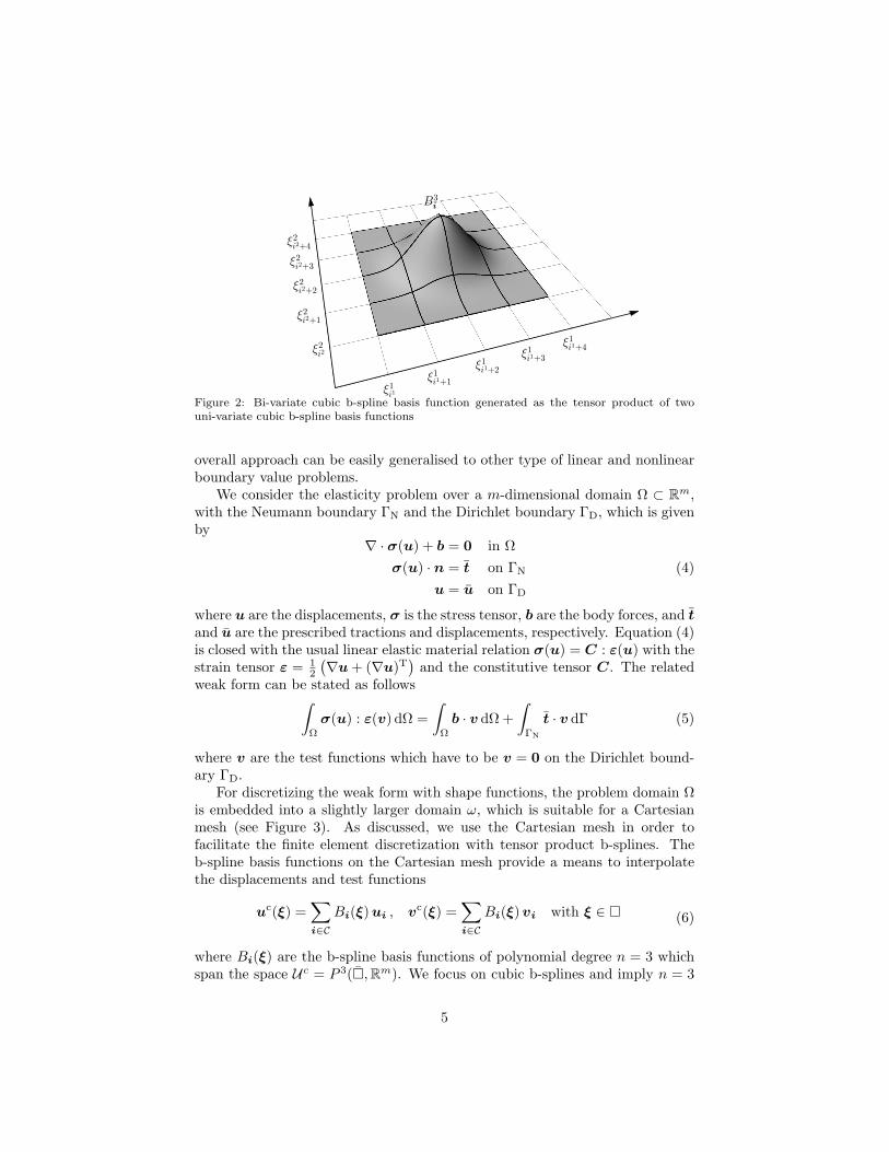
i (ξ1, ξ2) is depicted in Fig. 2.

3. B-spline finite elements

In the present paper, we restrict ourselves to linear second order boundaryvalue problems, namely elasticity and heat conduction. However, the presented

4

B3i

ξ1i1+1

ξ1i1+2

ξ1i1+3

ξ1i1+4

ξ1i1

ξ2i2

ξ2i2+1

ξ2i2+2

ξ2i2+3

ξ2i2+4

Figure 2: Bi-variate cubic b-spline basis function generated as the tensor product of twouni-variate cubic b-spline basis functions

overall approach can be easily generalised to other type of linear and nonlinearboundary value problems.

We consider the elasticity problem over a m-dimensional domain Ω ⊂ Rm,with the Neumann boundary ΓN and the Dirichlet boundary ΓD, which is givenby

∇ · σ(u) + b = 0 in Ωσ(u) · n = t on ΓN

u = u on ΓD

(4)

where u are the displacements, σ is the stress tensor, b are the body forces, and tand u are the prescribed tractions and displacements, respectively. Equation (4)is closed with the usual linear elastic material relation σ(u) = C : ε(u) with thestrain tensor ε = 1

2

(∇u + (∇u)T

)and the constitutive tensor C. The related

weak form can be stated as follows∫Ω

σ(u) : ε(v) dΩ =∫

Ω

b · v dΩ +∫

ΓN

t · v dΓ (5)

where v are the test functions which have to be v = 0 on the Dirichlet bound-ary ΓD.

For discretizing the weak form with shape functions, the problem domain Ωis embedded into a slightly larger domain ω, which is suitable for a Cartesianmesh (see Figure 3). As discussed, we use the Cartesian mesh in order tofacilitate the finite element discretization with tensor product b-splines. Theb-spline basis functions on the Cartesian mesh provide a means to interpolatethe displacements and test functions

uc(ξ) =∑i∈C

Bi(ξ) ui , vc(ξ) =∑i∈C

Bi(ξ) vi with ξ ∈ (6)

where Bi(ξ) are the b-spline basis functions of polynomial degree n = 3 whichspan the space Uc = P 3(, Rm). We focus on cubic b-splines and imply n = 3

5

∆x1∆x1

∆ξ1 ∆ξ1

Ω

x

ω

physical

©

ξ

parametric

∆x2

∆x2

ΓN

ΓD ∆ξ2

∆ξ2

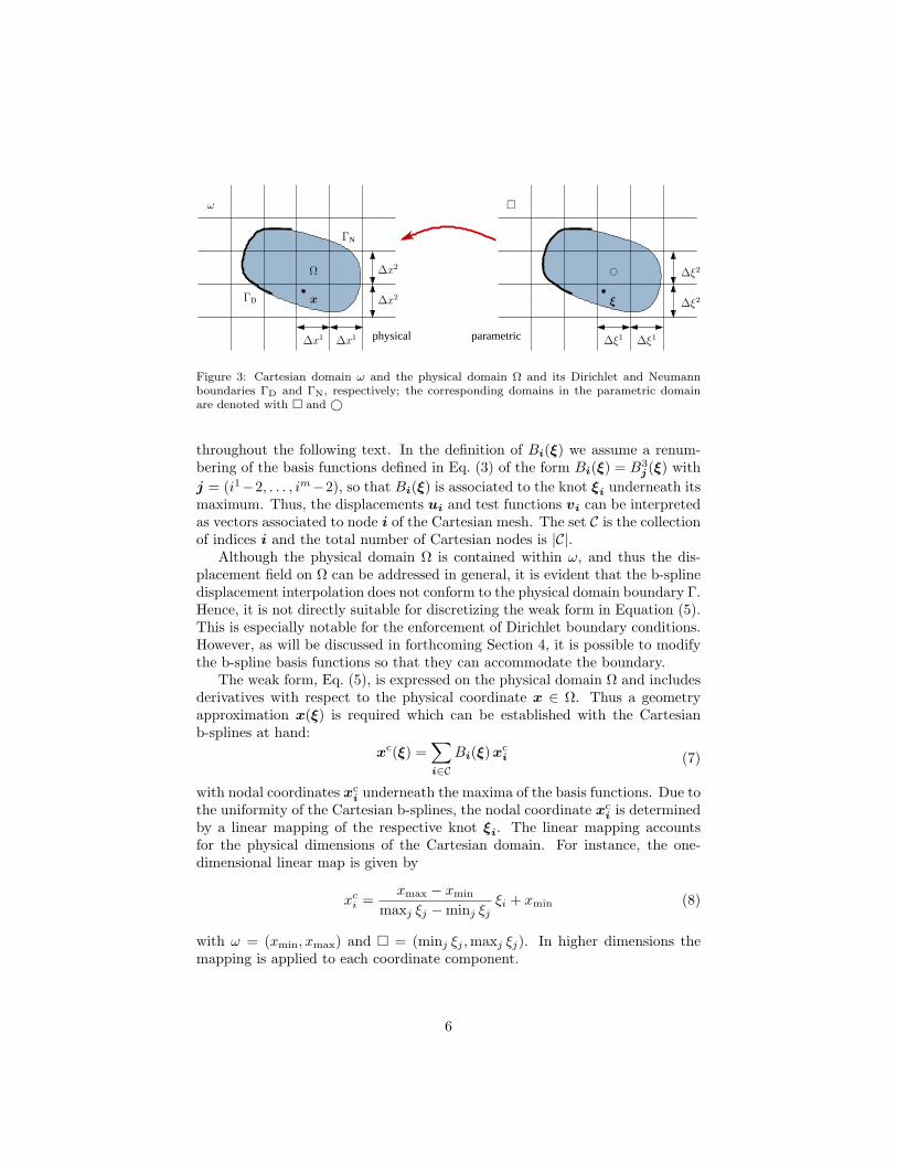
Figure 3: Cartesian domain ω and the physical domain Ω and its Dirichlet and Neumannboundaries ΓD and ΓN, respectively; the corresponding domains in the parametric domainare denoted with and ©

throughout the following text. In the definition of Bi(ξ) we assume a renum-bering of the basis functions defined in Eq. (3) of the form Bi(ξ) = B3

j (ξ) withj = (i1−2, . . . , im−2), so that Bi(ξ) is associated to the knot ξi underneath itsmaximum. Thus, the displacements ui and test functions vi can be interpretedas vectors associated to node i of the Cartesian mesh. The set C is the collectionof indices i and the total number of Cartesian nodes is |C|.

Although the physical domain Ω is contained within ω, and thus the dis-placement field on Ω can be addressed in general, it is evident that the b-splinedisplacement interpolation does not conform to the physical domain boundary Γ.Hence, it is not directly suitable for discretizing the weak form in Equation (5).This is especially notable for the enforcement of Dirichlet boundary conditions.However, as will be discussed in forthcoming Section 4, it is possible to modifythe b-spline basis functions so that they can accommodate the boundary.

The weak form, Eq. (5), is expressed on the physical domain Ω and includesderivatives with respect to the physical coordinate x ∈ Ω. Thus a geometryapproximation x(ξ) is required which can be established with the Cartesianb-splines at hand:

xc(ξ) =∑i∈C

Bi(ξ) xci (7)

with nodal coordinates xci underneath the maxima of the basis functions. Due to

the uniformity of the Cartesian b-splines, the nodal coordinate xci is determined

by a linear mapping of the respective knot ξi. The linear mapping accountsfor the physical dimensions of the Cartesian domain. For instance, the one-dimensional linear map is given by

xci =

xmax − xmin

maxj ξj −minj ξjξi + xmin (8)

with ω = (xmin, xmax) and = (minj ξj ,maxj ξj). In higher dimensions themapping is applied to each coordinate component.

6

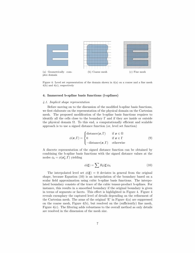
(a) Geometrically com-plex domain

(b) Coarse mesh (c) Fine mesh

Figure 4: Level set representation of the domain shown in 4(a) on a coarse and a fine mesh4(b) and 4(c), respectively

4. Immersed b-spline basis functions (i-splines)

4.1. Implicit shape representationBefore moving on to the discussion of the modified b-spline basis functions,

we first elaborate on the representation of the physical domain on the Cartesianmesh. The proposed modification of the b-spline basis functions requires toidentify all the cells close to the boundary Γ and if they are inside or outsidethe physical domain Ω. To this end, a computationally efficient and scalableapproach is to use a signed distance function (or, level set function)

φ(x,Γ) =

distance(x,Γ) if x ∈ Ω0 if x ∈ Γ−distance(x,Γ) otherwise

(9)

A discrete representation of the signed distance function can be obtained bycombining the b-spline basis functions with the signed distance values at thenodes φi = φ(xc

i,Γ) yielding

φ(ξ) =∑

Bi(ξ)φi (10)

The interpolated level set φ(ξ) = 0 deviates in general from the originalshape, because Equation (10) is an interpolation of the boundary based on ascalar field approximation using cubic b-spline basis functions. The interpo-lated boundary consists of the trace of the cubic tensor-product b-splines. Forinstance, this results in a smoothed boundary if the original boundary is givenin terms of segments or facets. This effect is highlighted in Figure 4. Figure 4reveals exemplary the captured level of details depending on the refinement ofthe Cartesian mesh. The arms of the original ‘E’ in Figure 4(a) are suppressedon the coarse mesh, Figure 4(b), but resolved on the (sufficiently) fine mesh,Figure 4(c). The filtering adds robustness to the overall method as only detailsare resolved in the dimension of the mesh size.

7

In contrast to the usual parametric mesh based boundary representations(using segments or facets), level set based representations are more suitable forproblems with large deformations and topology changes. There are efficientand scalable algorithms for converting a mesh based representation into an im-plicit representation (e.g., closest point transform [18, 19]) and vice versa (e.g.,marching cubes [20]).

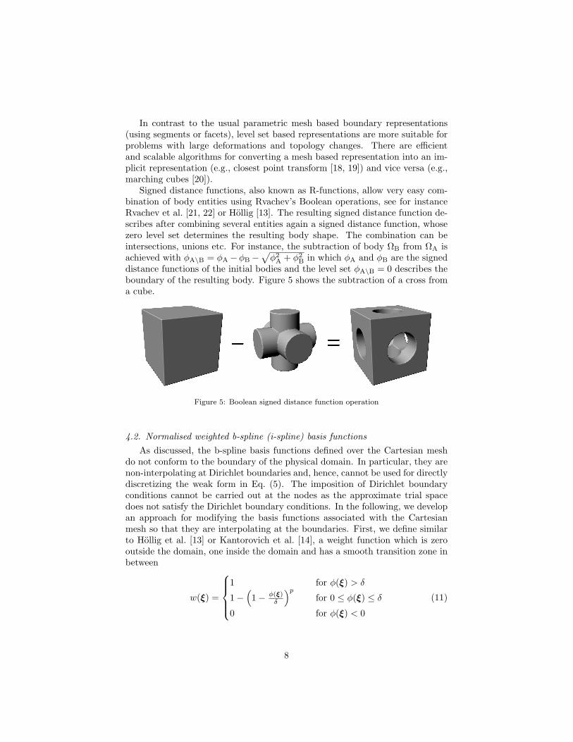
Signed distance functions, also known as R-functions, allow very easy com-bination of body entities using Rvachev’s Boolean operations, see for instanceRvachev et al. [21, 22] or Hollig [13]. The resulting signed distance function de-scribes after combining several entities again a signed distance function, whosezero level set determines the resulting body shape. The combination can beintersections, unions etc. For instance, the subtraction of body ΩB from ΩA isachieved with φA\B = φA−φB−

√φ2

A + φ2B in which φA and φB are the signed

distance functions of the initial bodies and the level set φA\B = 0 describes theboundary of the resulting body. Figure 5 shows the subtraction of a cross froma cube.

Figure 5: Boolean signed distance function operation

4.2. Normalised weighted b-spline (i-spline) basis functionsAs discussed, the b-spline basis functions defined over the Cartesian mesh

do not conform to the boundary of the physical domain. In particular, they arenon-interpolating at Dirichlet boundaries and, hence, cannot be used for directlydiscretizing the weak form in Eq. (5). The imposition of Dirichlet boundaryconditions cannot be carried out at the nodes as the approximate trial spacedoes not satisfy the Dirichlet boundary conditions. In the following, we developan approach for modifying the basis functions associated with the Cartesianmesh so that they are interpolating at the boundaries. First, we define similarto Hollig et al. [13] or Kantorovich et al. [14], a weight function which is zerooutside the domain, one inside the domain and has a smooth transition zone inbetween

w(ξ) =

1 for φ(ξ) > δ

1−(1− φ(ξ)

δ

)p

for 0 ≤ φ(ξ) ≤ δ

0 for φ(ξ) < 0

(11)

8

where φ(ξ) is the signed distance, δ is a transition length and p is an integerwith p ≥ 1 which controls the smoothness of the weight function inside thedomain. Inside the domain, the weight function gradient is non-zero and Cp−1-continuous including at φ(ξ) = δ. Advantageously, if we take p ≥ n, the weightdoes not interfere with the Cn−1-continuity of the b-splines.

4.2.1. Classification of cells and nodesAll the Cartesian mesh cells are tagged as physical, fictitious or boundary

depending on their position with respect to the physical domain. This classifi-cation is performed by computing for each cell e the minimum and maximumsigned distance, respectively. The collected different cell types form sub-domainsof the Cartesian domain, i.e.

physical = e ∈ | minξ∈e

φ(ξ) ≥ 0 (12a)

fictitious = e ∈ | maxξ∈e

φ(ξ) < 0 (12b)

boundary = \ (physical ∪fictitious) (12c)

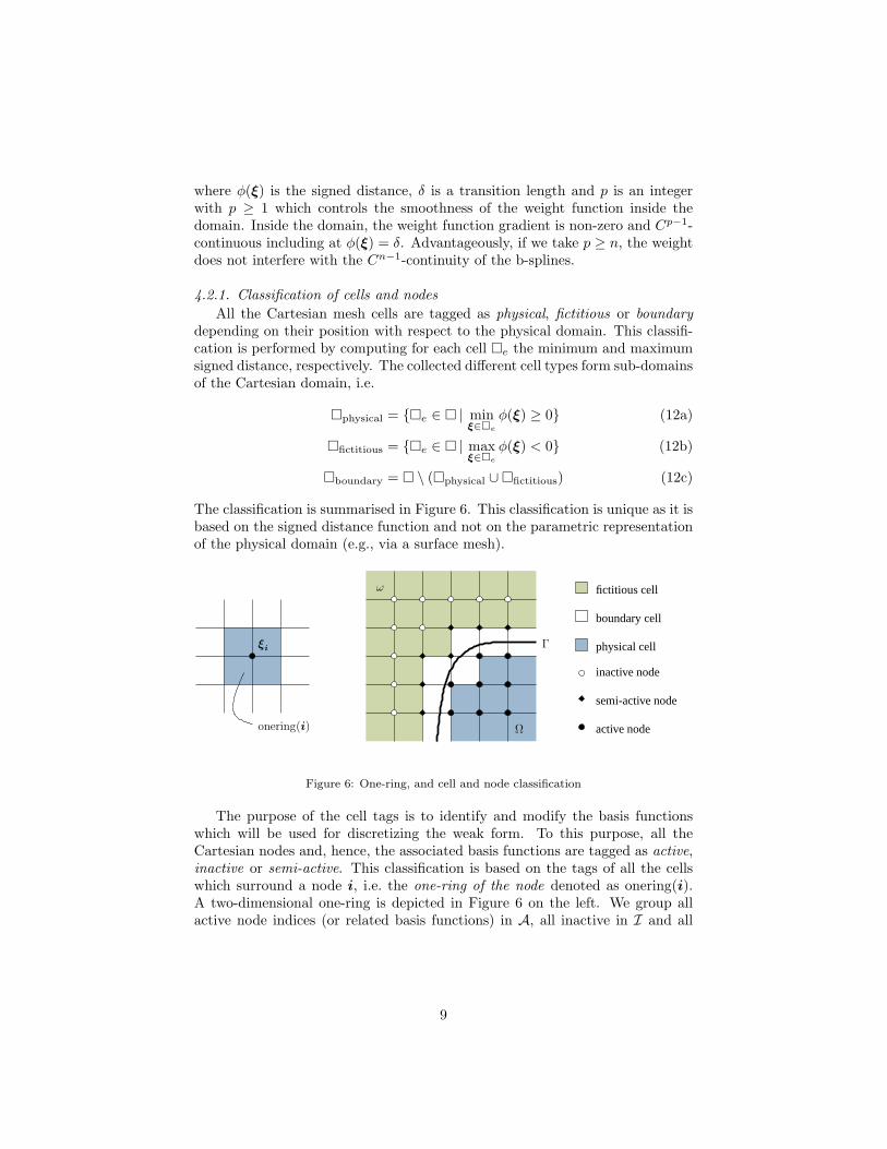
The classification is summarised in Figure 6. This classification is unique as it isbased on the signed distance function and not on the parametric representationof the physical domain (e.g., via a surface mesh).

fictitious cell

boundary cell

physical cell

inactive node

semi-active node

active nodeΩ

Γ

ω

onering(i)

ξi

Figure 6: One-ring, and cell and node classification

The purpose of the cell tags is to identify and modify the basis functionswhich will be used for discretizing the weak form. To this purpose, all theCartesian nodes and, hence, the associated basis functions are tagged as active,inactive or semi-active. This classification is based on the tags of all the cellswhich surround a node i, i.e. the one-ring of the node denoted as onering(i).A two-dimensional one-ring is depicted in Figure 6 on the left. We group allactive node indices (or related basis functions) in A, all inactive in I and all

9

semi-active in S which are given by

A = i ∈ C | onering(i) ⊂ (physical ∪boundary) (13a)I = i ∈ C | onering(i) ⊂ fictitious (13b)S = C \ (A ∪ I) (13c)

The node classification is shown in Figure 6. It is observable that an activenode contains only physical or boundary cells in its one-ring. However, a semi-active node is characterised by boundary and fictitious cells in its one-ring. Theremaining inactive nodes are only surrounded by fictitious cells.

4.2.2. Construction of i-spline basis functionsThe preceding definitions are used for defining a weighting function zi asso-

ciated with each node (or, basis function) i of the Cartesian mesh. Dependingon the classification, the nodal weighting function is set to

zi(ξ) =

w(ξ) if i ∈ A, i.e. node is active1 if i ∈ S, i.e. node is semi-active0 if i ∈ I, i.e. node is inactive

(14)

The weight function zi is a scalar field attached to each Cartesian node (orbasis function) i. The application of the weighting functions does not modifythe b-splines ziBi in the core of the domain Ω, because w attains the value1 there. However, the b-splines are altered whose support is intersected bythe boundary. Those reaching their maximum inside of Ω are forced to vanishon the boundary and outside of Ω. The semi-active b-splines, which reachtheir maximum just outside of Ω, are kept unchanged. The basis functionsbeing even farther outside are removed. The removal includes basis functionsthat have only small support in the physical domain, which may lead to badlyconditioned systems and stability problems.

Finally, the nodally weighted b-splines are adapted to yield a set of ba-sis functions interpolating at the immersed boundary, i.e. which are 1 on theboundary. This scaling is achieved by normalising the weighted b-splines ziBi.The normalisation of the weighted b-splines yields

Ni(ξ) =zi(ξ) Bi(ξ)∑j zj(ξ) Bj(ξ)

. (15)

The normalisation does not only ensure(∑

i Ni(ξ))|ξ∈∂© = 1, but also estab-

lishes a partition of unity. For the sake of brevity, these rationalised weighted b-splines are abbreviated with i-splines. Only the active and semi-active i-splinesare of interest, since inactivity leads to Ni = 0 for any i ∈ I.

The derived rationalised weighted b-splines span the approximate test space

Vh = vh ∈ Cn−1(©, Rm) |vh(ξ) =∑

i∈A∪SNNi(ξ)vi (16)

10

on the closed parametric domain © of the body, which would satisfy homoge-neous Dirichlet boundary conditions. The semi-active i-splines are separated intwo subsets SD ∪ SN = S. The basis functions Ni ∈ SD achieve their maximaon the Dirichlet boundary. The remaining semi-active basis functions are inSN. Satisfaction of in-homogeneous boundary conditions can be added to theapproximate trial space

Uh = Vh ⊕ uh ∈ Cn−1(©, Rm) |uh(ξ) =∑

i∈SDNi(ξ)ui (17)

using the semi-active basis functions in SD. The latter allow to impose theDirichlet boundary conditions at the nodes i ∈ SD like in ordinary finite el-ements based on Lagrangian polynomials, or by performing, a least-square fitwith respect to the Dirichlet data. Similar to Lagrangian finite elements, anoverlap region suppi∈SD

(Ni) ∩ suppj∈SN(Nj) 6= ∅ exists. In this region the

prescribed displacements blend with the unknown displacements.In summary, the i-spline basis is used to interpolate the displacements u and

test functions v, cf. Equation (6),

uh(ξ) =∑

i∈A∪S

Ni(ξ) ui and vh(ξ) =∑

i∈A∪SN

Ni(ξ) vi , (18)

since this approach allows to enforce the Dirichlet boundary conditions in a localway.

Illustration of one-dimensional i-splines. The construction process of the i-spline basis is illustrated with a one-dimensional model problem. Figures 7 to 9show the construction steps of the modified basis functions for a one-dimensionaldomain © = (0.9, 5.4) on the Cartesian domain = (−3, 9).

0

0.2

0.4

0.6

0.8

1

1.2

-3 -2 -1 0 1 2 3 4 5 6 7 8 9

Bi

ξ

w(ξ)

1 2 3 i=4 5 6 7 8 9 10 11 12 13

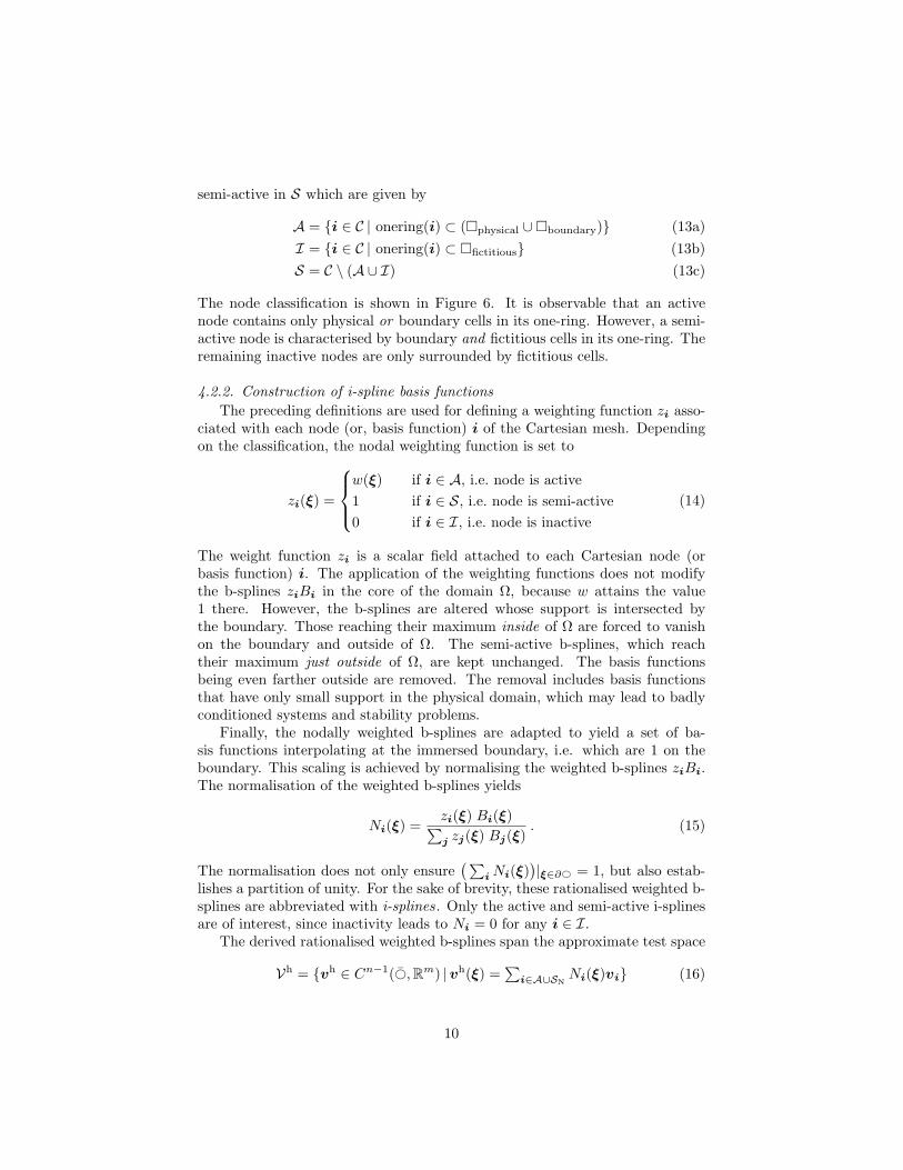
Figure 7: Model problem 1D: Cubic b-splines and a smooth weight function w(ξ) (with δ = 1,p = 3)

In Figure 7 the ordinary cubic b-splines are depicted, in which the relevantbasis functions i = 5, . . . , 10 in the immersed domain © = (0.9, 5.4) are drawnwith thicker lines. The weighting function w(x) with δ = 1 and p = 3 is shownas well. After multiplication with the weight functions zi(ξ) the shape of thefunctions i = 5, . . . , 9 are modified, cf. Figure 8. The support is reduced of the

11

0

0.2

0.4

0.6

0.8

1

1.2

-3 -2 -1 0 1 2 3 4 5 6 7 8 9

ziB

i

ξ

i=4

5

6 7 89

10

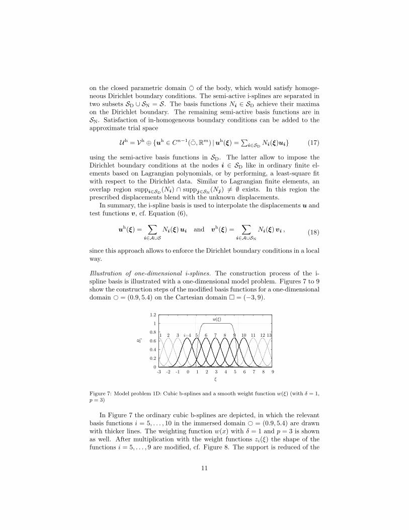
Figure 8: Model problem 1D: Weighted basis functions

0

0.2

0.4

0.6

0.8

1

1.2

-3 -2 -1 0 1 2 3 4 5 6 7 8 9

Ni

ξ

i=4

5 6 7 8 9

10

Figure 9: Model problem 1D: I-spline basis functions computed with the proposed approach.Note that the modified basis functions are interpolating at the boundaries.

functions close the boundary, namely z5B5, z6B6, z8B8 and z9B9. The basisfunctions z4B4 and z10B10 are kept unaltered. The support of at least oneCartesian integration cell is clearly observable. The two basis functions B3 andB11, which have a small support in the physical domain are removed. Finally,the normalisation elevates the semi-active basis functions z4B4 and z10B10 toone on the immersed boundary, see Figure 9. The process also scales the activebasis functions z5B5, . . . , z9B9. Although the central basis function N7 is slightlychanged in the depicted situation, it is straightforward to imagine a large enoughregion, in which core basis functions would remain literally unchanged.

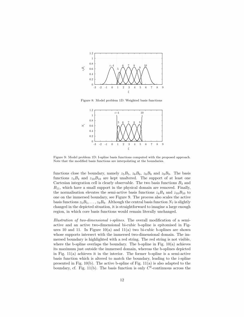
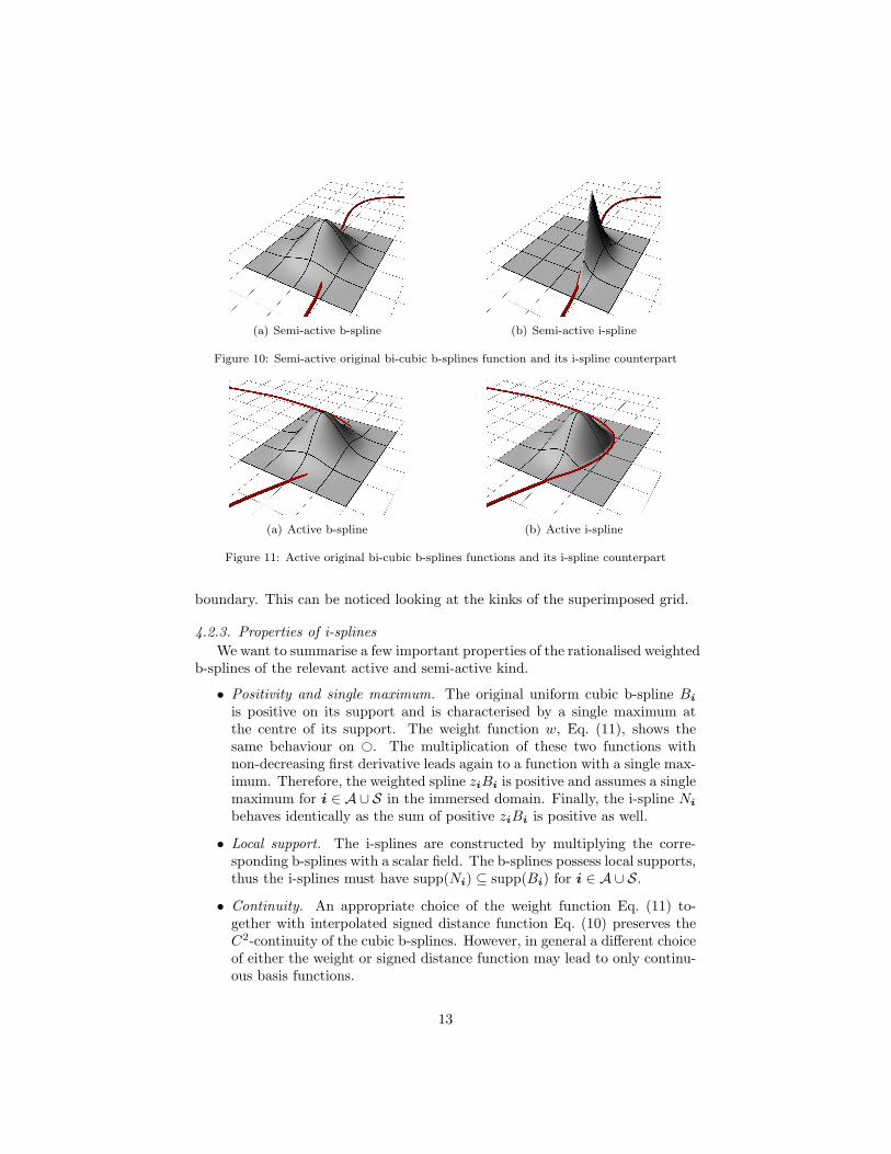
Illustration of two-dimensional i-splines. The overall modification of a semi-active and an active two-dimensional bi-cubic b-spline is epitomised in Fig-ures 10 and 11. In Figure 10(a) and 11(a) two bi-cubic b-splines are shownwhose supports intersect with the immersed two-dimensional domain. The im-mersed boundary is highlighted with a red string. The red string is not visible,where the b-spline overlaps the boundary. The b-spline in Fig. 10(a) achievesits maximum just outside the immersed domain, whereas the b-splines depictedin Fig. 11(a) achieves it in the interior. The former b-spline is a semi-activebasis function which is altered to match the boundary, leading to the i-splinepresented in Fig. 10(b). The active b-spline of Fig. 11(a) is also adapted to theboundary, cf. Fig. 11(b). The basis function is only C0-continuous across the

12

(a) Semi-active b-spline (b) Semi-active i-spline

Figure 10: Semi-active original bi-cubic b-splines function and its i-spline counterpart

(a) Active b-spline (b) Active i-spline

Figure 11: Active original bi-cubic b-splines functions and its i-spline counterpart

boundary. This can be noticed looking at the kinks of the superimposed grid.

4.2.3. Properties of i-splinesWe want to summarise a few important properties of the rationalised weighted

b-splines of the relevant active and semi-active kind.

• Positivity and single maximum. The original uniform cubic b-spline Bi

is positive on its support and is characterised by a single maximum atthe centre of its support. The weight function w, Eq. (11), shows thesame behaviour on ©. The multiplication of these two functions withnon-decreasing first derivative leads again to a function with a single max-imum. Therefore, the weighted spline ziBi is positive and assumes a singlemaximum for i ∈ A ∪ S in the immersed domain. Finally, the i-spline Ni

behaves identically as the sum of positive ziBi is positive as well.

• Local support. The i-splines are constructed by multiplying the corre-sponding b-splines with a scalar field. The b-splines possess local supports,thus the i-splines must have supp(Ni) ⊆ supp(Bi) for i ∈ A ∪ S.

• Continuity. An appropriate choice of the weight function Eq. (11) to-gether with interpolated signed distance function Eq. (10) preserves theC2-continuity of the cubic b-splines. However, in general a different choiceof either the weight or signed distance function may lead to only continu-ous basis functions.

13

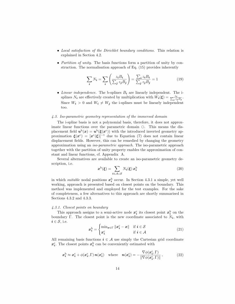
• Local satisfaction of the Dirichlet boundary conditions. This relation isexplained in Section 4.2.

• Partition of unity. The basis functions form a partition of unity by con-struction. The normalisation approach of Eq. (15) provides inherently

∑i

Ni =∑

i

(ziBi∑j zjBj

)=∑

i ziBi∑j zjBj

= 1 (19)

• Linear independence. The b-splines Bi are linearly independent. The i-splines Ni are effectively created by multiplication with Wi(ξ) = ziP

j zjBj.

Since Wi > 0 and Wi 6= Wj the i-splines must be linearly independenttoo.

4.3. Iso-parametric geometry representation of the immersed domainThe i-spline basis is not a polynomial basis, therefore, it does not approx-

imate linear functions over the parametric domain ©. This means the dis-placement field uh(x) = uh(ξ(xc)) with the introduced inverted geometry ap-proximation ξ(xc) = [xc(ξ)]−1 due to Equation (7) does not contain lineardisplacement fields. However, this can be remedied by changing the geometryapproximation using an iso-parametric approach. The iso-parametric approachtogether with the partition of unity property enables the approximation of con-stant and linear functions, cf. Appendix A.

Several alternatives are available to create an iso-parametric geometry de-scription, i.e.

xh(ξ) =∑

i∈A∪S

Ni(ξ) xhi (20)

in which suitable nodal positions xhi occur. In Section 4.3.1 a simple, yet well

working, approach is presented based on closest points on the boundary. Thismethod was implemented and employed for the test examples. For the sakeof completeness, a few alternatives to this approach are shortly summarised inSections 4.3.2 and 4.3.3.

4.3.1. Closest points on boundaryThis approach assigns to a semi-active node xc

i its closest point xhi on the

boundary Γ. The closest point is the new coordinate associated to Ni, withi ∈ S, i.e.

xhi =

minx∈Γ ‖xc

i − x‖ if i ∈ Sxc

i if i ∈ A(21)

All remaining basis functions i ∈ A use simply the Cartesian grid coordinatexc

i. The closest points xhi can be conveniently estimated with

xhi ≈ xc

i + φ(xci,Γ) n(xc

i) where n(xci) = − ∇φ(xc

i,Γ)‖∇φ(xc

i,Γ)‖, (22)

14

Γ

Ω

ω

(a) Closest points of semi-activeCartesian nodes

Ω

Γ

(b) Mesh after change to iso-parametric node coordinates

fictitious cell

boundary cell

physical cell

inactive node

semi-active node

active node

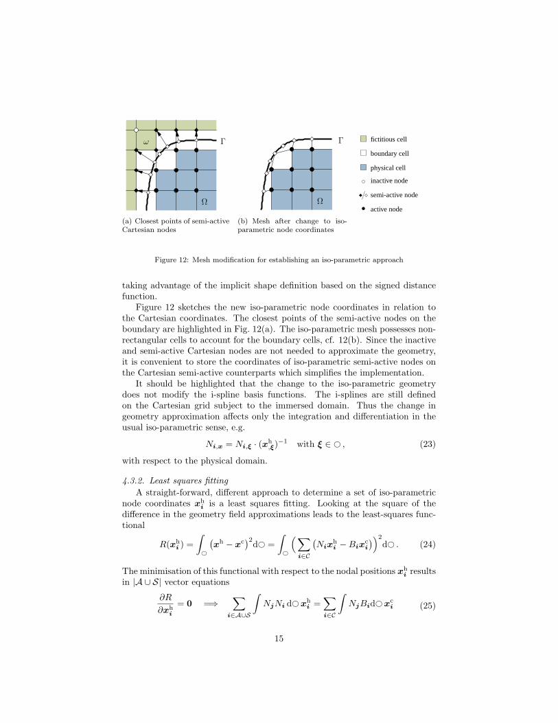
Figure 12: Mesh modification for establishing an iso-parametric approach

taking advantage of the implicit shape definition based on the signed distancefunction.

Figure 12 sketches the new iso-parametric node coordinates in relation tothe Cartesian coordinates. The closest points of the semi-active nodes on theboundary are highlighted in Fig. 12(a). The iso-parametric mesh possesses non-rectangular cells to account for the boundary cells, cf. 12(b). Since the inactiveand semi-active Cartesian nodes are not needed to approximate the geometry,it is convenient to store the coordinates of iso-parametric semi-active nodes onthe Cartesian semi-active counterparts which simplifies the implementation.

It should be highlighted that the change to the iso-parametric geometrydoes not modify the i-spline basis functions. The i-splines are still definedon the Cartesian grid subject to the immersed domain. Thus the change ingeometry approximation affects only the integration and differentiation in theusual iso-parametric sense, e.g.

Ni,x = Ni,ξ · (xh,ξ)

−1 with ξ ∈ © , (23)

with respect to the physical domain.

4.3.2. Least squares fittingA straight-forward, different approach to determine a set of iso-parametric

node coordinates xhi is a least squares fitting. Looking at the square of the

difference in the geometry field approximations leads to the least-squares func-tional

R(xhi ) =

∫©

(xh − xc

)2d© =∫©

(∑i∈C

(Nix

hi −Bix

ci

))2

d© . (24)

The minimisation of this functional with respect to the nodal positions xhi results

in |A ∪ S| vector equations

∂R

∂xhi

= 0 =⇒∑

i∈A∪S

∫NjNi d©xh

i =∑i∈C

∫NjBid©xc

i (25)

15

The method has the drawback to violate the interpolation on the boundary, sincethe residuum is minimised on the whole body domain, contradicting the originaltarget. The linear system can be reduced by setting xh

i = xci for all active nodes

i ∈ A only computing the semi-active node coordinates. Alternatively, only thegeometry difference over the domain boundary could be considered.

4.3.3. At maximaAnother possibility to determine an appropriate set of coordinates xh

i canbe based on the maxima of the i-splines, i.e.

xhi =

∑j

Bj(ξmaxi )xc

j with ξmaxi = max

ξ∈©Ni(ξ) . (26)

The maximum of an i-spline can be easily detected and it is a priori known thatonly a single maximum exists for each i-spline on the domain ©. In terms ofcomputing the maxima, it appears convenient to convert (26) in a constraintminimisation problem,

ξmaxi = min

ξ∈supp Bi

φ(ξ)≥0

(−Ni(ξ)

), (27)

which limits the search region by incorporating the effective domain with thesigned distance function. Suitable algorithms can be found, e.g., in Nocedal andWright [23]. The parametric maximum ξi of the related original cubic b-splineprovides a good initial guess for iterative algorithms.

4.3.4. Numerical comparisonsIn Figure 13, the results of the presented identification methods of the iso-

parametric nodes are depicted for the one-dimensional model problem on © =[0.9, 5.4]. The closest point approach is denoted with CP, least squares fittingwith LS and underneath the maxima with AM. The reference solution is x =ξ. The least squares fitting violates the boundary which can be observed by

1

2

3

4

5

5.4

0.9 1 2 3 4 5 5.4

x

ξ

0.8

1.4

0.9 1.2

ξLS

AMCP

Figure 13: Iso-parametric geometry approximation of 1D model problem

16

looking at the magnified, boxed region. The AM curve satisfies the boundary,but exhibits relatively large deviation from the linear reference curve. Overall,the closest point approach appears to produce the best result. It ought tobe highlighted, in general, all presented approximations are viable since theyprovide a strictly positive gradient x,ξ. In essence, the positivity and the singlemaximum of the i-splines behaves rather good-natured towards modification ofthe nodal Cartesian coordinates as long as xh

i < xhi+1.

Although, the two-dimensional iso-parametric mesh shown in Figure 12 isbased on the closest point method, the least square fitting or AM techniquewould result in similarly distributed iso-parametric meshes. The shape of theiso-parametric mesh is a consequence of the iso-parametric geometry approxima-tion based on i-splines rather than of the method to determine the iso-parametricnode coordinates.

4.4. QuadratureThe integrals in the weak form (5) are given on the physical body domain Ω

and its Neumann boundary ΓN. Due to the (iso-)parametric description of thegeometry the integrals are mapped to the parametric body domain ©. This isa sub-domain on which the cubic b-splines are described; the b-splines and thei-splines share the parameters ξ. For instance, the integral of the external bodyforces results in∫

Ω

vh · b(x) dΩ =∫©

vh(ξ) · b(xh(ξ)) det(xh,ξ) d©

=∑

e

∑i∈A∪SN

vi ẩe

Ni(ξ) b(xh(ξ)) det(xh,ξ) d© ,

(28)

in which the parametric body domain © =⋃

e©e is the collection of the inte-

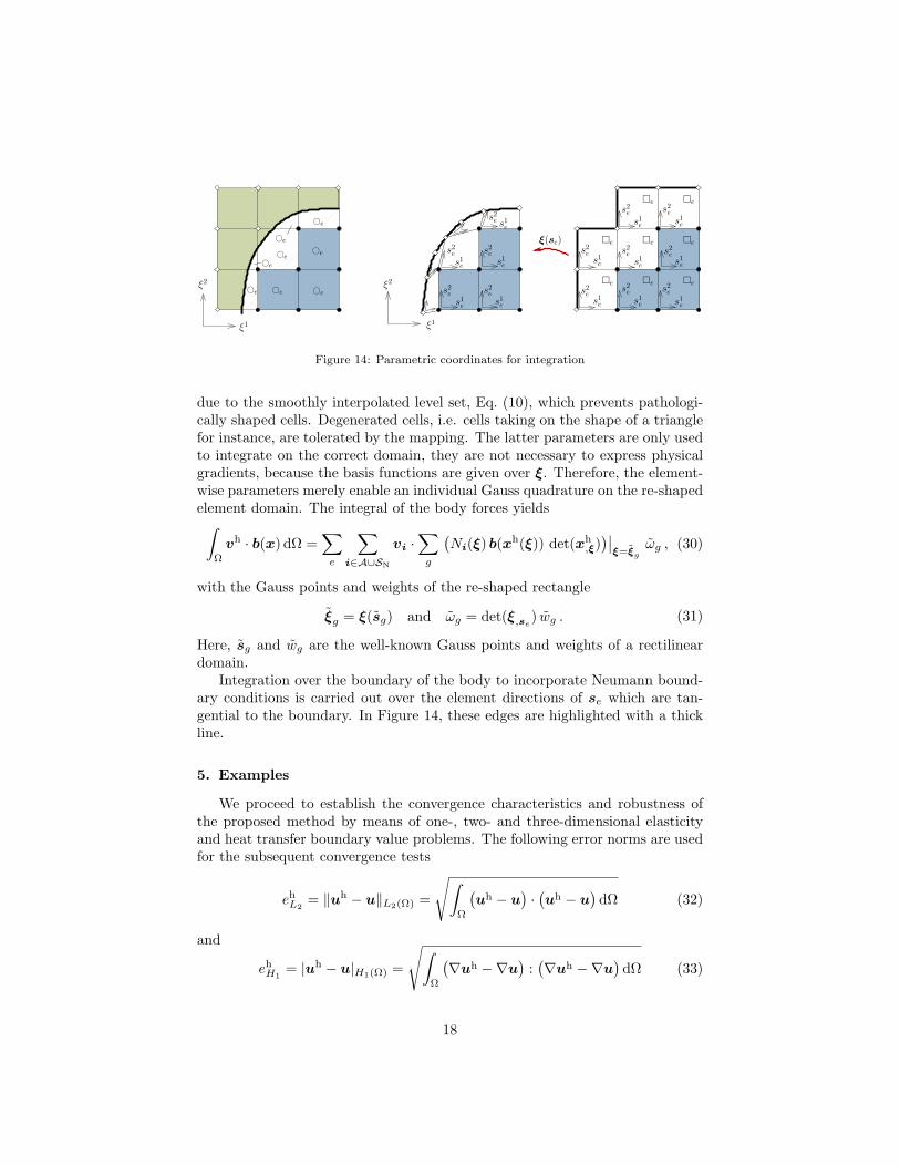
gration cells ©e. The cells are sketched on the left in Figure 14.Although it is possible to integrate on the physical cells, for which ©e = e,

directly with an ordinary Gauss quadrature, this cannot be performed on bound-ary cells characterised by ©e ⊂ e. However, the iso-parametric geometrymapping allows to consider each boundary cell as a re-shaped Cartesian cell.Additional element-wise parameters se are introduced on each element, cf. Fig-ure 14, and mapped to ξ using the cubic b-splines

ξ(se) =∑i∈Ke

Bi(se) ξhi with ξh

i = ξi + G ·(xh

i − xci

)and se ∈ e ,

(29)where Ke = i ∈ A ∪ S | supp(Bi) ∩ e 6= ∅ and in two dimensions G =diag( ∆ξ1

∆x1 , ∆ξ2

∆x2 ) with physical and parametric Cartesian mesh sizes ∆x1, ∆x2

and ∆ξ1 = ∆ξ2 = 1, respectively, see also Fig. 3. The one- and three-dimensional case follow analogously. Alternatively, the cubic b-splines can bereplaced by linear Lagrangian polynomials, however, the numerical examples ledto better results using cubic b-splines. The map ξ(se) behaves good-natured

17

ξ(se)

ξ2

ξ1ξ1

s1e

s2e

s1e

s2e

©e

©e

©e

©e

©e

©e

ξ2

s1e

s1e

s1e

s1e

s2e

s2e

s2e

s2e

s1e

s1e

s1e

s1e

s2e

s2e

s2e

©e

©e

s1e

s1e

s1e

s2e

s2e

s2e

s2e

e

ee

ee

e ee

Figure 14: Parametric coordinates for integration

due to the smoothly interpolated level set, Eq. (10), which prevents pathologi-cally shaped cells. Degenerated cells, i.e. cells taking on the shape of a trianglefor instance, are tolerated by the mapping. The latter parameters are only usedto integrate on the correct domain, they are not necessary to express physicalgradients, because the basis functions are given over ξ. Therefore, the element-wise parameters merely enable an individual Gauss quadrature on the re-shapedelement domain. The integral of the body forces yields∫

Ω

vh · b(x) dΩ =∑

e

∑i∈A∪SN

vi ·∑

g

(Ni(ξ) b(xh(ξ)) det(xh

,ξ))∣∣

ξ=ξgωg , (30)

with the Gauss points and weights of the re-shaped rectangle

ξg = ξ(sg) and ωg = det(ξ,se) wg . (31)

Here, sg and wg are the well-known Gauss points and weights of a rectilineardomain.

Integration over the boundary of the body to incorporate Neumann bound-ary conditions is carried out over the element directions of se which are tan-gential to the boundary. In Figure 14, these edges are highlighted with a thickline.

5. Examples

We proceed to establish the convergence characteristics and robustness ofthe proposed method by means of one-, two- and three-dimensional elasticityand heat transfer boundary value problems. The following error norms are usedfor the subsequent convergence tests

ehL2

= ‖uh − u‖L2(Ω) =

√∫Ω

(uh − u

)·(uh − u

)dΩ (32)

and

ehH1

= |uh − u|H1(Ω) =

√∫Ω

(∇uh −∇u

):(∇uh −∇u

)dΩ (33)

18

1e-06

1e-05

1e-04

1e-03

1e-02

1e-01

1e+00

0.001 0.01 0.1 1

error e

h

mesh size h

1

2

eh

L2

eh

H1

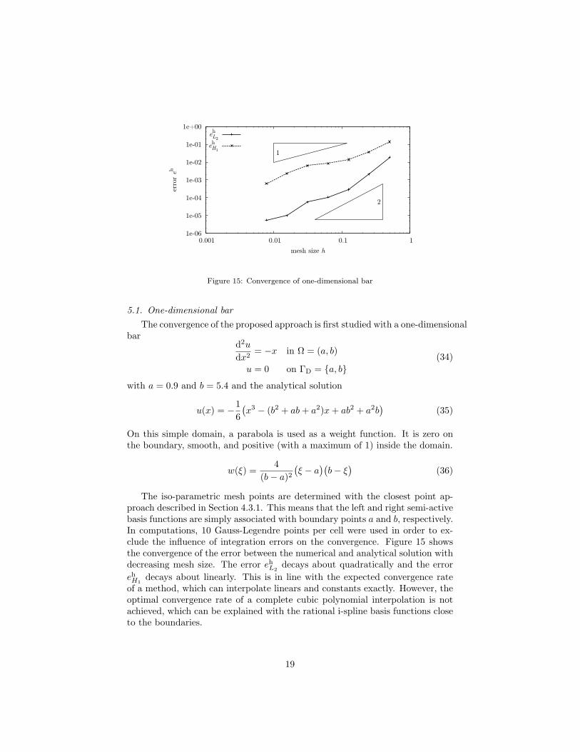
Figure 15: Convergence of one-dimensional bar

5.1. One-dimensional barThe convergence of the proposed approach is first studied with a one-dimensional

bard2u

dx2= −x in Ω = (a, b)

u = 0 on ΓD = a, b(34)

with a = 0.9 and b = 5.4 and the analytical solution

u(x) = −16(x3 − (b2 + ab + a2)x + ab2 + a2b

)(35)

On this simple domain, a parabola is used as a weight function. It is zero onthe boundary, smooth, and positive (with a maximum of 1) inside the domain.

w(ξ) =4

(b− a)2(ξ − a

)(b− ξ

)(36)

The iso-parametric mesh points are determined with the closest point ap-proach described in Section 4.3.1. This means that the left and right semi-activebasis functions are simply associated with boundary points a and b, respectively.In computations, 10 Gauss-Legendre points per cell were used in order to ex-clude the influence of integration errors on the convergence. Figure 15 showsthe convergence of the error between the numerical and analytical solution withdecreasing mesh size. The error eh

L2decays about quadratically and the error

ehH1

decays about linearly. This is in line with the expected convergence rateof a method, which can interpolate linears and constants exactly. However, theoptimal convergence rate of a complete cubic polynomial interpolation is notachieved, which can be explained with the rational i-spline basis functions closeto the boundaries.

19

ΓN

Ω

R0

R1

ΓD

x2

x1

(a) Geometry (b) Mesh

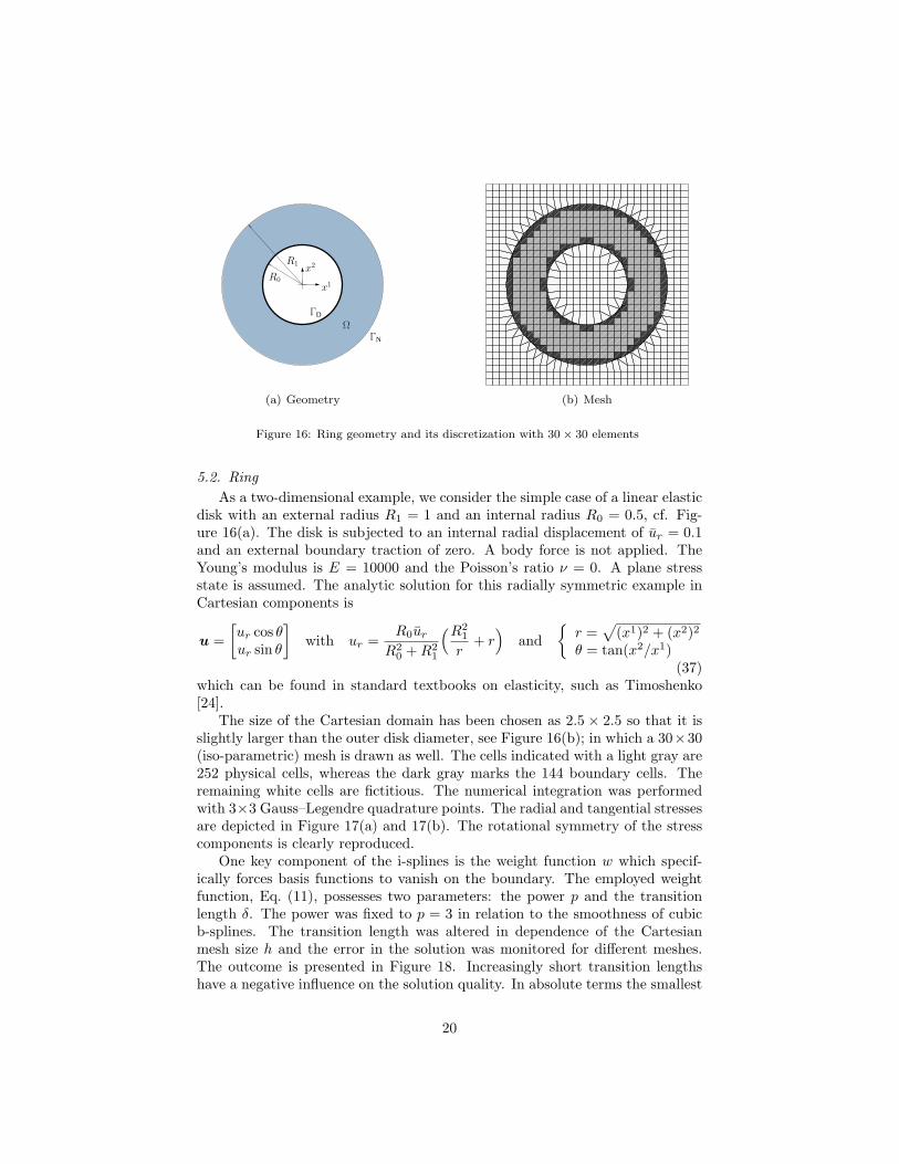
Figure 16: Ring geometry and its discretization with 30× 30 elements

5.2. RingAs a two-dimensional example, we consider the simple case of a linear elastic

disk with an external radius R1 = 1 and an internal radius R0 = 0.5, cf. Fig-ure 16(a). The disk is subjected to an internal radial displacement of ur = 0.1and an external boundary traction of zero. A body force is not applied. TheYoung’s modulus is E = 10000 and the Poisson’s ratio ν = 0. A plane stressstate is assumed. The analytic solution for this radially symmetric example inCartesian components is

u =[ur cos θur sin θ

]with ur =

R0ur

R20 + R2

1

(R21

r+ r)

and

r =√

(x1)2 + (x2)2θ = tan(x2/x1)

(37)which can be found in standard textbooks on elasticity, such as Timoshenko[24].

The size of the Cartesian domain has been chosen as 2.5 × 2.5 so that it isslightly larger than the outer disk diameter, see Figure 16(b); in which a 30×30(iso-parametric) mesh is drawn as well. The cells indicated with a light gray are252 physical cells, whereas the dark gray marks the 144 boundary cells. Theremaining white cells are fictitious. The numerical integration was performedwith 3×3 Gauss–Legendre quadrature points. The radial and tangential stressesare depicted in Figure 17(a) and 17(b). The rotational symmetry of the stresscomponents is clearly reproduced.

One key component of the i-splines is the weight function w which specif-ically forces basis functions to vanish on the boundary. The employed weightfunction, Eq. (11), possesses two parameters: the power p and the transitionlength δ. The power was fixed to p = 3 in relation to the smoothness of cubicb-splines. The transition length was altered in dependence of the Cartesianmesh size h and the error in the solution was monitored for different meshes.The outcome is presented in Figure 18. Increasingly short transition lengthshave a negative influence on the solution quality. In absolute terms the smallest

20

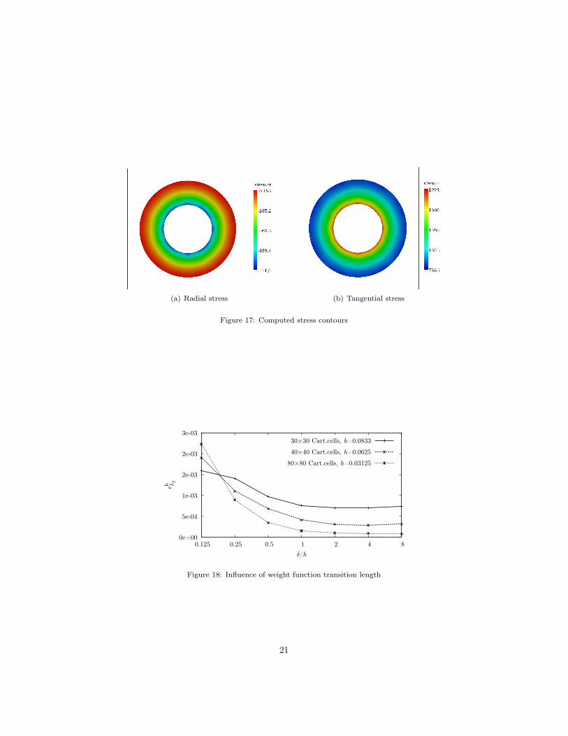
(a) Radial stress (b) Tangential stress

Figure 17: Computed stress contours

0e+00

5e-04

1e-03

2e-03

2e-03

3e-03

0.125 0.25 0.5 1 2 4 8

eh L

2

δ/h

30×30 Cart.cells, h=0.0833

40×40 Cart.cells, h=0.0625

80×80 Cart.cells, h=0.03125

Figure 18: Influence of weight function transition length

21

0.07

0.08

0.09

0.1

0.5 0.6 0.7 0.8 0.9 1

radia

l dis

pla

cem

ent

ur

radius r

analytic30×3040×4080×80

-1500

-1000

-500

0

500

1000

1500

2000

2500

0.5 0.625 0.75 0.875 1

stre

ss σ

rr, σ

θθ

radius r

σθθ

σrr

analytic30×3040×4080×80

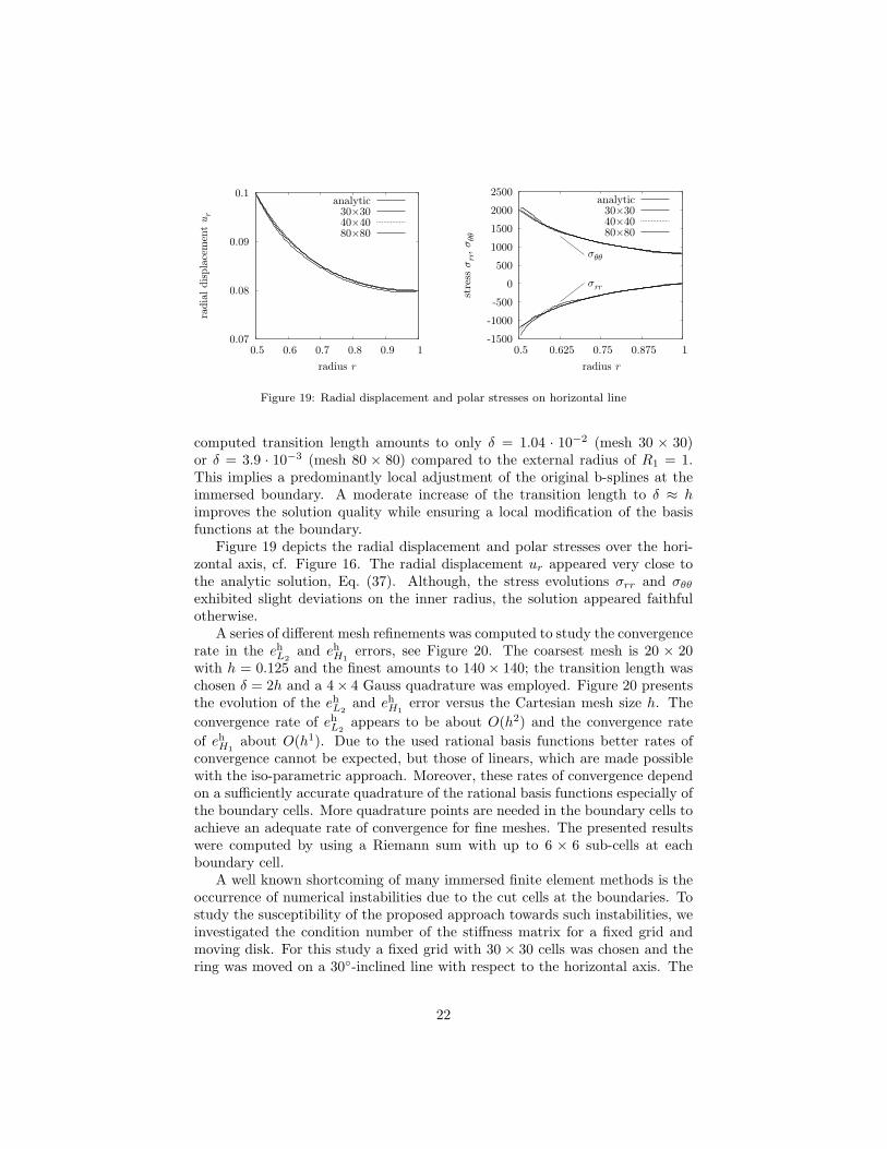
Figure 19: Radial displacement and polar stresses on horizontal line

computed transition length amounts to only δ = 1.04 · 10−2 (mesh 30 × 30)or δ = 3.9 · 10−3 (mesh 80 × 80) compared to the external radius of R1 = 1.This implies a predominantly local adjustment of the original b-splines at theimmersed boundary. A moderate increase of the transition length to δ ≈ himproves the solution quality while ensuring a local modification of the basisfunctions at the boundary.

Figure 19 depicts the radial displacement and polar stresses over the hori-zontal axis, cf. Figure 16. The radial displacement ur appeared very close tothe analytic solution, Eq. (37). Although, the stress evolutions σrr and σθθ

exhibited slight deviations on the inner radius, the solution appeared faithfulotherwise.

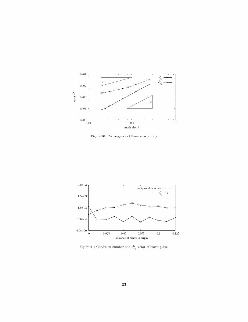
A series of different mesh refinements was computed to study the convergencerate in the eh

L2and eh

H1errors, see Figure 20. The coarsest mesh is 20 × 20

with h = 0.125 and the finest amounts to 140 × 140; the transition length waschosen δ = 2h and a 4× 4 Gauss quadrature was employed. Figure 20 presentsthe evolution of the eh

L2and eh

H1error versus the Cartesian mesh size h. The

convergence rate of ehL2

appears to be about O(h2) and the convergence rateof eh

H1about O(h1). Due to the used rational basis functions better rates of

convergence cannot be expected, but those of linears, which are made possiblewith the iso-parametric approach. Moreover, these rates of convergence dependon a sufficiently accurate quadrature of the rational basis functions especially ofthe boundary cells. More quadrature points are needed in the boundary cells toachieve an adequate rate of convergence for fine meshes. The presented resultswere computed by using a Riemann sum with up to 6 × 6 sub-cells at eachboundary cell.

A well known shortcoming of many immersed finite element methods is theoccurrence of numerical instabilities due to the cut cells at the boundaries. Tostudy the susceptibility of the proposed approach towards such instabilities, weinvestigated the condition number of the stiffness matrix for a fixed grid andmoving disk. For this study a fixed grid with 30× 30 cells was chosen and thering was moved on a 30-inclined line with respect to the horizontal axis. The

22

1e-05

1e-04

1e-03

1e-02

1e-01

0.01 0.1 1

error e

h

mesh size h

1

2

eh

L2

eh

H1

Figure 20: Convergence of linear-elastic ring

0.0e+00

5.0e-04

1.0e-03

1.5e-03

2.0e-03

0 0.025 0.05 0.075 0.1 0.125

distance of center to origin

recip.cond.numb.est.

eh

L2

Figure 21: Condition number and ehL2

error of moving disk

23

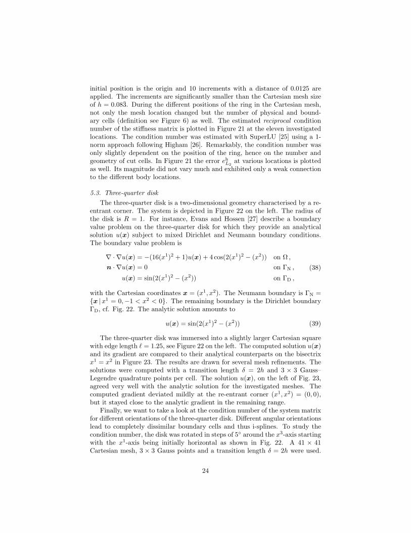
initial position is the origin and 10 increments with a distance of 0.0125 areapplied. The increments are significantly smaller than the Cartesian mesh sizeof h = 0.083. During the different positions of the ring in the Cartesian mesh,not only the mesh location changed but the number of physical and bound-ary cells (definition see Figure 6) as well. The estimated reciprocal conditionnumber of the stiffness matrix is plotted in Figure 21 at the eleven investigatedlocations. The condition number was estimated with SuperLU [25] using a 1-norm approach following Higham [26]. Remarkably, the condition number wasonly slightly dependent on the position of the ring, hence on the number andgeometry of cut cells. In Figure 21 the error eh

L2at various locations is plotted

as well. Its magnitude did not vary much and exhibited only a weak connectionto the different body locations.

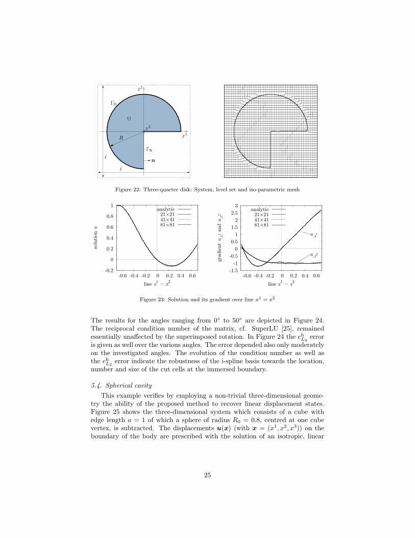
5.3. Three-quarter diskThe three-quarter disk is a two-dimensional geometry characterised by a re-

entrant corner. The system is depicted in Figure 22 on the left. The radius ofthe disk is R = 1. For instance, Evans and Hossen [27] describe a boundaryvalue problem on the three-quarter disk for which they provide an analyticalsolution u(x) subject to mixed Dirichlet and Neumann boundary conditions.The boundary value problem is

∇ · ∇u(x) = −(16(x1)2 + 1)u(x) + 4 cos(2(x1)2 − (x2)) on Ω ,n · ∇u(x) = 0 on ΓN ,

u(x) = sin(2(x1)2 − (x2)) on ΓD ,

(38)

with the Cartesian coordinates x = (x1, x2). The Neumann boundary is ΓN =x |x1 = 0,−1 < x2 < 0. The remaining boundary is the Dirichlet boundaryΓD, cf. Fig. 22. The analytic solution amounts to

u(x) = sin(2(x1)2 − (x2)) (39)

The three-quarter disk was immersed into a slightly larger Cartesian squarewith edge length ` = 1.25, see Figure 22 on the left. The computed solution u(x)and its gradient are compared to their analytical counterparts on the bisectrixx1 = x2 in Figure 23. The results are drawn for several mesh refinements. Thesolutions were computed with a transition length δ = 2h and 3 × 3 Gauss–Legendre quadrature points per cell. The solution u(x), on the left of Fig. 23,agreed very well with the analytic solution for the investigated meshes. Thecomputed gradient deviated mildly at the re-entrant corner (x1, x2) = (0, 0),but it stayed close to the analytic gradient in the remaining range.

Finally, we want to take a look at the condition number of the system matrixfor different orientations of the three-quarter disk. Different angular orientationslead to completely dissimilar boundary cells and thus i-splines. To study thecondition number, the disk was rotated in steps of 5 around the x3-axis startingwith the x1-axis being initially horizontal as shown in Fig. 22. A 41 × 41Cartesian mesh, 3 × 3 Gauss points and a transition length δ = 2h were used.

24

Ω

ΓD

ΓN

R

n

x2

ℓ

ℓ

x3

x1

Figure 22: Three-quarter disk: System, level set and iso-parametric mesh

-0.2

0

0.2

0.4

0.6

0.8

1

-0.6 -0.4 -0.2 0 0.2 0.4 0.6

solu

tion u

line x1 = x

2

analytic21×2141×4181×81

-1.5

-1

-0.5

0

0.5

1

1.5

2

2.5

3

-0.6 -0.4 -0.2 0 0.2 0.4 0.6

gra

die

nt

u,x

1 a

nd u

,x2

line x1 = x

2

u,x

1

u,x

2

analytic21×2141×4181×81

Figure 23: Solution and its gradient over line x1 = x2

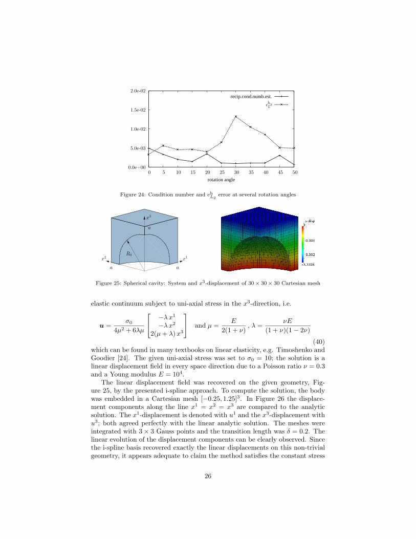
The results for the angles ranging from 0 to 50 are depicted in Figure 24.The reciprocal condition number of the matrix, cf. SuperLU [25], remainedessentially unaffected by the superimposed rotation. In Figure 24 the eh

L2error

is given as well over the various angles. The error depended also only moderatelyon the investigated angles. The evolution of the condition number as well asthe eh

L2error indicate the robustness of the i-spline basis towards the location,

number and size of the cut cells at the immersed boundary.

5.4. Spherical cavityThis example verifies by employing a non-trivial three-dimensional geome-

try the ability of the proposed method to recover linear displacement states.Figure 25 shows the three-dimensional system which consists of a cube withedge length a = 1 of which a sphere of radius R0 = 0.8, centred at one cubevertex, is subtracted. The displacements u(x) (with x = (x1, x2, x3)) on theboundary of the body are prescribed with the solution of an isotropic, linear

25

0.0e+00

5.0e-03

1.0e-02

1.5e-02

2.0e-02

0 5 10 15 20 25 30 35 40 45 50

rotation angle

recip.cond.numb.est.

eh

L2

Figure 24: Condition number and ehL2

error at several rotation angles

x3

R0

a a

a

x2

x1

Figure 25: Spherical cavity: System and x3-displacement of 30× 30× 30 Cartesian mesh

elastic continuum subject to uni-axial stress in the x3-direction, i.e.

u =σ0

4µ2 + 6λµ

−λ x1

−λ x2

2(µ + λ) x3

and µ =E

2(1 + ν), λ =

νE

(1 + ν)(1− 2ν)

(40)which can be found in many textbooks on linear elasticity, e.g. Timoshenko andGoodier [24]. The given uni-axial stress was set to σ0 = 10; the solution is alinear displacement field in every space direction due to a Poisson ratio ν = 0.3and a Young modulus E = 104.

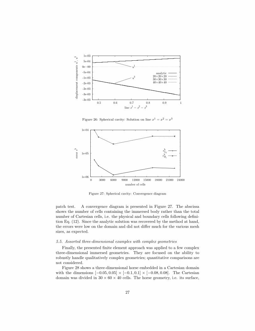
The linear displacement field was recovered on the given geometry, Fig-ure 25, by the presented i-spline approach. To compute the solution, the bodywas embedded in a Cartesian mesh [−0.25, 1.25]3. In Figure 26 the displace-ment components along the line x1 = x2 = x3 are compared to the analyticsolution. The x1-displacement is denoted with u1 and the x3-displacement withu3; both agreed perfectly with the linear analytic solution. The meshes wereintegrated with 3× 3 Gauss points and the transition length was δ = 0.2. Thelinear evolution of the displacement components can be clearly observed. Sincethe i-spline basis recovered exactly the linear displacements on this non-trivialgeometry, it appears adequate to claim the method satisfies the constant stress

26

-3e-03

-3e-03

-2e-03

-2e-03

-1e-03

-5e-04

0e+00

5e-04

1e-03

0.5 0.6 0.7 0.8 0.9 1

dis

pla

cem

ent

com

ponen

ts u

1, u

3

line x1 = x

2 = x

3

u1

u3

analytic20×20×2030×30×3040×40×40

Figure 26: Spherical cavity: Solution on line x1 = x2 = x3

1e-06

1e-05

1e-04

0 3000 6000 9000 12000 15000 18000 21000 24000

error e

h

number of cells

eh

L2

eh

H1

Figure 27: Spherical cavity: Convergence diagram

patch test. A convergence diagram is presented in Figure 27. The abscissashows the number of cells containing the immersed body rather than the totalnumber of Cartesian cells, i.e. the physical and boundary cells following defini-tion Eq. (12). Since the analytic solution was recovered by the method at hand,the errors were low on the domain and did not differ much for the various meshsizes, as expected.

5.5. Assorted three-dimensional examples with complex geometriesFinally, the presented finite element approach was applied to a few complex

three-dimensional immersed geometries. They are focused on the ability torobustly handle qualitatively complex geometries; quantitative comparisons arenot considered.

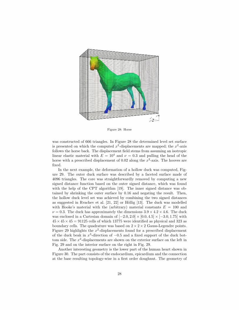
Figure 28 shows a three-dimensional horse embedded in a Cartesian domainwith the dimensions [−0.05, 0.05] × [−0.1, 0.1] × [−0.08, 0.08]. The Cartesiandomain was divided in 30 × 60 × 40 cells. The horse geometry, i.e. its surface,

27

x3

x1

x2

Figure 28: Horse

was constructed of 666 triangles. In Figure 28 the determined level set surfaceis presented on which the computed x2-displacements are mapped; the x2-axisfollows the horse back. The displacement field stems from assuming an isotropiclinear elastic material with E = 104 and ν = 0.3 and pulling the head of thehorse with a prescribed displacement of 0.02 along the x2-axis. The hooves arefixed.

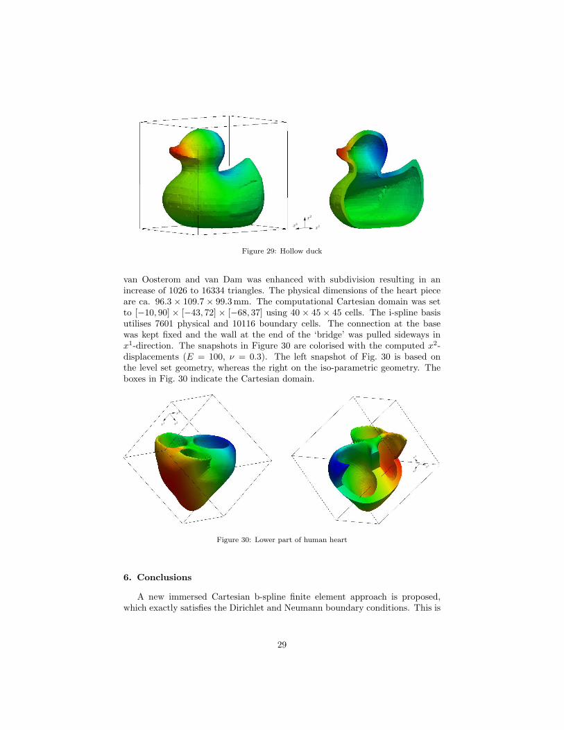
In the next example, the deformation of a hollow duck was computed, Fig-ure 29. The outer duck surface was described by a faceted surface made of4096 triangles. The core was straightforwardly removed by computing a newsigned distance function based on the outer signed distance, which was foundwith the help of the CPT algorithm [19]. The inner signed distance was ob-tained by shrinking the outer surface by 0.16 and negating the result. Then,the hollow duck level set was achieved by combining the two signed distancesas suggested in Rvachev et al. [21, 22] or Hollig [13]. The duck was modelledwith Hooke’s material with the (arbitrary) material constants E = 100 andν = 0.3. The duck has approximately the dimensions 3.9× 4.2× 4.6. The duckwas enclosed in a Cartesian domain of [−2.0, 2.0]× [0.0, 4.5]× [−3.0, 1.75] with45× 45× 45 = 91125 cells of which 13775 were identified as physical and 323 asboundary cells. The quadrature was based on 2× 2× 2 Gauss-Legendre points.Figure 29 highlights the x2-displacements found for a prescribed displacementof the duck beak in x3-direction of −0.5 and a fixed support of the duck bot-tom side. The x2-displacements are shown on the exterior surface on the left inFig. 29 and on the interior surface on the right in Fig. 29.

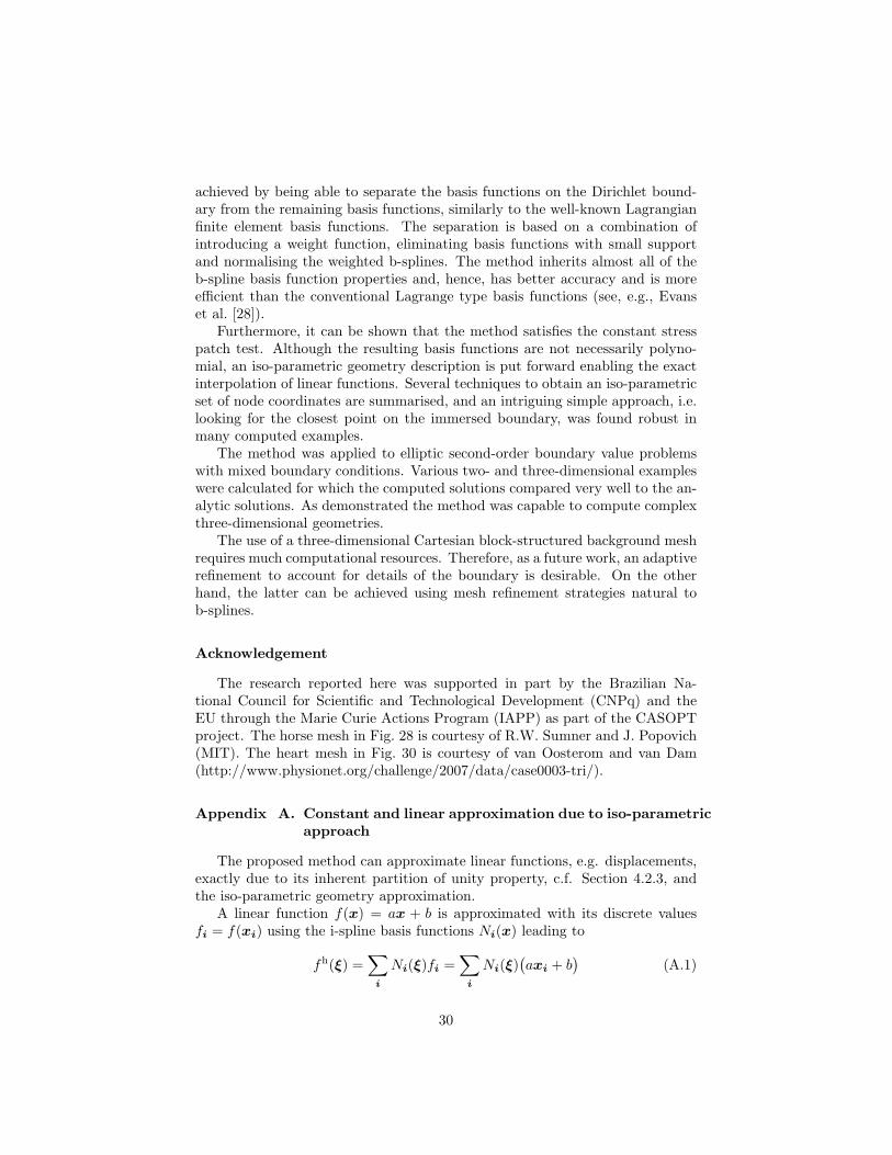
Another interesting geometry is the lower part of the human heart shown inFigure 30. The part consists of the endocardium, epicardium and the connectionat the base resulting topology-wise in a first order doughnut. The geometry of

28

x1

x2

x3

Figure 29: Hollow duck

van Oosterom and van Dam was enhanced with subdivision resulting in anincrease of 1026 to 16334 triangles. The physical dimensions of the heart pieceare ca. 96.3 × 109.7 × 99.3 mm. The computational Cartesian domain was setto [−10, 90] × [−43, 72] × [−68, 37] using 40 × 45 × 45 cells. The i-spline basisutilises 7601 physical and 10116 boundary cells. The connection at the basewas kept fixed and the wall at the end of the ‘bridge’ was pulled sideways inx1-direction. The snapshots in Figure 30 are colorised with the computed x2-displacements (E = 100, ν = 0.3). The left snapshot of Fig. 30 is based onthe level set geometry, whereas the right on the iso-parametric geometry. Theboxes in Fig. 30 indicate the Cartesian domain.

x1

x2

x3

x1

x2

x3

Figure 30: Lower part of human heart

6. Conclusions

A new immersed Cartesian b-spline finite element approach is proposed,which exactly satisfies the Dirichlet and Neumann boundary conditions. This is

29

achieved by being able to separate the basis functions on the Dirichlet bound-ary from the remaining basis functions, similarly to the well-known Lagrangianfinite element basis functions. The separation is based on a combination ofintroducing a weight function, eliminating basis functions with small supportand normalising the weighted b-splines. The method inherits almost all of theb-spline basis function properties and, hence, has better accuracy and is moreefficient than the conventional Lagrange type basis functions (see, e.g., Evanset al. [28]).

Furthermore, it can be shown that the method satisfies the constant stresspatch test. Although the resulting basis functions are not necessarily polyno-mial, an iso-parametric geometry description is put forward enabling the exactinterpolation of linear functions. Several techniques to obtain an iso-parametricset of node coordinates are summarised, and an intriguing simple approach, i.e.looking for the closest point on the immersed boundary, was found robust inmany computed examples.

The method was applied to elliptic second-order boundary value problemswith mixed boundary conditions. Various two- and three-dimensional exampleswere calculated for which the computed solutions compared very well to the an-alytic solutions. As demonstrated the method was capable to compute complexthree-dimensional geometries.

The use of a three-dimensional Cartesian block-structured background meshrequires much computational resources. Therefore, as a future work, an adaptiverefinement to account for details of the boundary is desirable. On the otherhand, the latter can be achieved using mesh refinement strategies natural tob-splines.

Acknowledgement

The research reported here was supported in part by the Brazilian Na-tional Council for Scientific and Technological Development (CNPq) and theEU through the Marie Curie Actions Program (IAPP) as part of the CASOPTproject. The horse mesh in Fig. 28 is courtesy of R.W. Sumner and J. Popovich(MIT). The heart mesh in Fig. 30 is courtesy of van Oosterom and van Dam(http://www.physionet.org/challenge/2007/data/case0003-tri/).

Appendix A. Constant and linear approximation due to iso-parametricapproach

The proposed method can approximate linear functions, e.g. displacements,exactly due to its inherent partition of unity property, c.f. Section 4.2.3, andthe iso-parametric geometry approximation.

A linear function f(x) = ax + b is approximated with its discrete valuesfi = f(xi) using the i-spline basis functions Ni(x) leading to

fh(ξ) =∑

i

Ni(ξ)fi =∑

i

Ni(ξ)(axi + b

)(A.1)

30

Although this approximation is not in general linear over ξ, it is still linear overthe iso-parametric approximation of the coordinate xh(ξ) =

∑i Ni(ξ)xi. The

preserved linearity over xh(ξ) can be seen by expanding Equation (A.1)

fh(ξ) = a∑

i

Ni(ξ)xi︸ ︷︷ ︸= xh(ξ)

+b∑

i

Ni(ξ)︸ ︷︷ ︸= 1

, (A.2)

which yields the desired result fh(xh) = axh + b after dropping the parametriccoordinates.

References

[1] T. Hughes, J. Cottrell, Y. Bazilevs, Isogeometric analysis: CAD, finite ele-ments, NURBS, exact geometry and mesh refinement, Computer Methodsin Applied Mechanics and Engineering 194 (2005) 4135–4195.

[2] F. Cirak, M. Ortiz, P. Schroder, Subdivision surfaces: a new paradigmfor thin-shell finite-element analysis, International Journal for NumericalMethods in Engineering 47 (2000) 2039–2072.

[3] J. Peters, U. Reif, Subdivision surfaces, Springer Verlag, 2008.

[4] J. Warren, H. Weimer, Subdivision methods for geometric design: a con-structive approach, Morgan Kaufmann, 2001.

[5] F. Cirak, M. Scott, E. Antonsson, M. Ortiz, P. Schroder, Integrated model-ing, finite-element analysis, and engineering design for thin-shell structuresusing subdivision, Computer-Aided Design 34 (2002) 137–148.

[6] J. Cottrell, T. Hughes, Y. Bazilevs, Isogeometric analysis: toward integra-tion of CAD and FEA, John Wiley & Sons Ltd., 2009.

[7] H. Prautzsch, W. Boehm, M. Paluszny, Bezier and b-spline techniques,Springer Verlag, 2002.

[8] C. De Boor, K. Hollig, S. Riemenschneider, Box splines, Springer Verlag,1993.

[9] R. Glowinski, T.-W. Pan, J. Periaux, A fictitious domain method forDirichlet problem and applications, Computer Methods in Applied Me-chanics and Engineering 111 (1994) 283–303.

[10] C. Peskin, The immersed boundary method, Acta Numerica 11 (2002)479–517.

[11] T. Belytschko, C. Parimi, N. Moes, N. Sukumar, S. Usui, Structured ex-tended finite element methods for solids defined by implicit surfaces, Inter-national Journal for Numerical Methods in Engineering 56 (2003) 609–635.

31

[12] K. Hollig, U. Reif, J. Wipper, Weighted extended b-spline approximationof dirichlet problems, SIAM Journal on Numerical Analysis 39 (2002) 442–462.

[13] K. Hollig, Finite element methods with b-splines, SIAM, Philadelphia,2003.

[14] L. W. Kantorovich, W. I. Krylov, Approximate methods of higher analysis,Interscience Publishers, New York, translated from the 4th Rusian edition,1964.

[15] L. Piegl, W. Tiller, The NURBS book, Springer, 1997.

[16] D. Rogers, An introduction to NURBS, Academic Press, 2001.

[17] C. de Boor, A practical guide to splines, Springer-Verlag, New York, revisededition, 2001.

[18] S. Mauch, Efficient algorithms for solving static Hamilton-Jacobi equations,Ph.D. thesis, California Institute of Technology, 2003.

[19] F. Cirak, R. Deiterding, S. Mauch, Large-scale fluid-structure interactionsimulation of viscoplastic and fracturing thin-shells subjected to shocks anddetonations, Computers & Structures 85 (2007) 1049–1065.

[20] W. Lorensen, H. E. Cline, Marching cubes: a high resolution 3d surfaceconstruction algorithm, Computer Graphics 21 (1987) 163–169.

[21] V. L. Rvachev, T. I. Sheiko, R-functions in boundary value problems inmechanics, Applied Mechanics Reviews 48 (1995) 151–188.

[22] V. L. Rvachev, T. I. Sheiko, V. Shapiro, I. Tsukanov, On completeness ofRFM solution structures, Computational Mechanics 25 (2000) 305–317.

[23] J. Nocedal, S. J. Wright, Numerical optimization, Springer, 2nd edition,2000.

[24] S. Timoshenko, J. N. Goodier, Theory of elasticity, McGraw-Hill HigherEducation, 3rd edition, 1970.

[25] J. W. Demmel, J. R. Gilbert, X. S. Li, SuperLU users’ guide, Technical Re-port LBNL-44289, Lawrence Berkeley National Lab, Berkeley, CA, U.S.A.,2009.

[26] N. J. Higham, Accuracy and stability of numerical algorithms, SIAM,Philadelphia, PA, U.S.A., 1996.

[27] D. J. Evans, K. A. A. Hossen, The numerical solution of problems involv-ing singularities by the finite element method, International Journal ofComputer Mathematics 19 (1986) 339–379.

32

[28] J. Evans, Y. Bazilevs, I. Babuska, T. Hughes, n-widths, sup-infs, and op-timality ratios for the k-version of the isogeometric finite element method,Computer Methods in Applied Mechanics and Engineering 198 (2009)1726–1741.

33