Transform Coding

National Chiao Tung University

Chun-Jen Tsai

11/24/2014

2/36

Transform Domain Data Analysis

� Given an invertible transform A, the entropy of a

source x does not change subject to A, i.e. Ax has the

same entropy as x.

� However, there are several reasons why we want to perform lossy compression on Ax, instead of x:

� Input data sequence can be interpreted with more insights

� Input data possibly are de-correlated in transform domain

� The original time-ordered sequence of data can be decomposed into different categories

3/36

Example: Height-Weight Data (1/3)

� The height-weight data pair tends to cluster alone the line xh = 2.5xw. A rotation transform

can simplify the data representation :

,02.68,cossin

sincoso=

−= φ

φφ

φφA

xh

xw

=

w

h

x

xA

1

0

θ

θ

θ1

θ0

4/36

Example: Height-Weight Data (2/3)

� If we set θ1 to zeros for all the data pairs, and transform the data back to xh–xw domain, we have the

reconstruction errors as follows:

Original data Reconstructed data

5/36

Example: Height-Weight Data (3/3)

� Note that, in original data, both xh and xw have non-

negligible variances, however, for θ0 and θ1, only θ0

has large variance

� Variance (or energy) of a source and its information

has a positive relation; larger source variance, higher

entropy

� For Gaussian source, the differential entropy is (log2πeσ2)/2.

� The error introduced into the reconstructed sequence of {x} is equal to the error introduced into the

transform-domain sequence {θ}.

6/36

Transform Coding Principle

� Transform step:

� The source {xn} is divided into blocks of size N. Each block is

mapped into a transform sequence {en} using a reversible mapping

� Most of the energy of the transformed block was contained in few

elements of the transformed values

� Quantization step:

� The transformed sequence is quantized based on the following

strategy:

� The desired average bit rate

� The statistics of the various transformed elements

� The effect of distortion on the reconstructed sequence

� Entropy coding step:

� The quantized data are entropy-coded using Huffman, AC, or other

techniques

7/36

Transform Formulation

� For media coding, only linear transforms are used

� The forward transform can be denoted by

� The inverse transform is

� The selection of N is application-specific

� Complexity of transform is lower for small N

� Large N adapts to fast-changing statistics badly

� Large N produces better resolution in transform domain

.1

0

,∑−

=

=N

i

inin axθ

.1

0

,∑−

=

=N

i

inin bx θ

8/36

2-D Forward Transform

� For 2-D signals Xi,j, a general linear 2-D transform of

block size N×N is given as

� If separable transform is used; the formulation can be

simplified to

� In matrix form, the separable transform becomes

ΘΘΘΘ = AXAT.

.1

0

1

0

,,,,, ∑∑−

=

−

=

=ΘN

i

N

j

lkjijilk ax

.1

0

1

0

,,,

1

0

1

0

,,,, ∑ ∑∑∑−

=

−

=

−

=

−

=

==Θ

N

i

N

j

ljjiik

N

i

N

j

ljjiiklk axaaxa

9/36

Orthonormal Transform

� All the transforms used in multimedia compression are orthonormal transforms. Thus, A–1 = AT.

In this case, ΘΘΘΘ = AXAT becomes ΘΘΘΘ = AXA–1.

� Orthonormal transforms are energy preserving

.

)(

1

0

2

1

0

2

∑

∑−

=

−

=

===

==

N

n

n

TTT

TTN

i

i

xxxAxAx

AxAxθθθ

10/36

Energy Compaction Effect

� The efficiency of a transform depends on how much

energy compaction is provided by the transform

� The amount of energy compaction can be measured

by the ratio of the arithmetic mean of the variances to

their geometric means:

where σi2 is the variance of the ith coefficients.

( ),

121

0

1

0

21

N

i

N

i

N

i iN

TCGσ

σ

−=

−

=

Π=∑

Note: The wider the spread of σi2 w.r.t. their arithmetic mean, the smaller the value of the geometric mean

will be → better energy compaction!

11/36

Decomposition of 1-D Input

� Transform decomposes an input sequence into

components with different characteristics. If

input x = [x1, x2], the transformed output is

The first transformed component computes the

average (i.e. low-pass) behavior of the input

sequence, while the 2nd component captures the

differential (i.e. high-pass) behavior of the input.

,11

11

2

1

−=A

.2

)(,

2

)( 2121

−+=

xxxxAx

12/36

Decomposition of 2-D Input

� If A in previous example is used for 2-D transform

and X is a 2-D input, we have X = ATΘA:

where αi,j is the outer product of ith and jth rows of A.

� How do you interpret θ0,0, …, θ1,1?

� θ0,0 is the DC coefficient, and other θi,j are AC coefficients.

,

2

1

11

11

11

11

2

1

1,1110,1101,0010,000

1110010011100100

1110010011100100

1110

0100

1110

0100

αθαθαθαθ

θθθθθθθθ

θθθθθθθθ

θθ

θθ

+++=

+−−−−+

−+−+++=

−

−=

xx

xx

13/36

Karhunen-Loeve Transform (KLT)

� KLT consists of the eigenvectors of the autocorrelation matrix: [R]i,j = E[XnXn+|i–j|].

� KLT minimizes the geometric means of the variance of the transform coefficients → provides maximal GTC

� Issues with KLT

� For non-stationary inputs, the autocorrelation function is time varying; computation of KLT is relatively expensive

� KLT matrix must be transmitted to the decoder

� If the input statistics change slowly, and the transform size can be kept small, the KLT can be useful

14/36

Example: KLT

� For N = 2, the autocorrelation matrix for a stationary

process is

The eigenvectors of R are

With orthonormal constraint, the transform matrix is

.11

11

2

1

−=K

,)0()1(

)1()0(

=

xxxx

xxxx

RR

RRR

., 21

−=

=

β

β

α

αvv

15/36

Discrete Cosine Transform

� DCT is derived from the Discrete Fourier Transform

(DFT) by first perform an even-function extension to

the input data, then compute its DFT:

� Only real number operations are required

� Better energy compaction than DFT

DFT

DCT

16/36

DCT Formulation

� The rows of DCT matrix is composed of cosine

functions of different frequencies:

� The inner product of the input signal with each row of

the matrix is the projection of the input signal onto a

cosine function of fixed frequency

� The larger N is, the better the frequency resolution is

[ ] .1,...,1,0,1,...,1

1,...,1,0,0

2

)12(cos

2

)12(cos

2

1

,−=−=

−==

+

+

=NjNi

Nji

N

jiN

ji

C

N

N

ji π

π

17/36

Basis Functions of 8-Point DCT

� Each column of the DCT matrix is a basis function:

18/36

Basis Images of 8-Point 2-D DCT

� DCT can be extended to a 2-D transform:

19/36

Performance of DCT

� For Markov sources with high correlation coefficient ρ,

the compaction ability of DCT is close to that of KLT

� As many sources can be modeled as Markov sources

with high values for ρ, DCT is the most popular

transform for multimedia compression

[ ],

][ 2

1

n

nn

xE

xxE +=ρ

20/36

Discrete Walsh-Hadamard Trans.

� The Hadamard transform is defined by an N×N

matrix H with the property HHT = NI.

� Simple to compute while still separate low frequency from high frequency components of the input data

� The Hadamard matrix is recursively defined as:

� The DWHT transform matrix is obtained by

� Normalize the matrix by 1/N½ so that it is orthonormal

� Re-arrange the rows according to number of sign changes

].1[and, 12 =

−= H

HH

HHH

NN

NN

N

21/36

Coding of Transform Coefficients

� Different transform coefficients should be quantized

and coded differently based on the amount of

information it carries

� Information is related to the variance of each coefficients

� The bit allocation problem tries to determine the level

of quantizer to use for different transform coefficients

� The Lagrange multiplier optimization technique is

often used to solve the optimal bit allocation

22/36

Lagrange Multiplier

� A constrained optimization problem tries to minimize a cost function f(x, y) subject to some constraints on

the parameter x and y: g(x, y) = c

� The Lagrange cost function is defined as follows:

� Solution: solve

.),(),(),,(2

cyxgyxfyxJ −⋅−= λλ

0

5

10

15

20

25

0

5

10

15

20

25

-8

-6

-4

-2

0

2

4

6

8

.0),,(,, =∇ λλ yxJyx

23/36

Rate-Distortion Optimization (1/3)

� If the rate per coefficient is R and the rate per kth

coefficient is Rk , then

where M is the number of transform coefficients

� The error variance for the kth quantizer σrk

2, is related

to the kth input variance σθk

2, by:

where αk depends on input distribution and quantizer

� The total reconstruction error is given by

,1

1

∑=

=M

k

kRM

R

,2 222

k

k

k

R

kr θσασ −=

.21

222 ∑=

−=M

k

R

kr k

k

θσασ

24/36

Rate-Distortion Optimization (2/3)

� The objective of the bit allocation procedure is to find Rk to minimize σr

2 subject to total rate constraint R.

� If we assume that αk is a constant α for all k, we can

set up the minimization problem in terms of Lagrange

multipliers as

� Taking the derivative of J with respect to Rk and

setting it to zero, we obtain the expression for Rk:

.1

211

22

−−= ∑∑

==

−M

k

k

M

k

RR

MRJ

k

k λσα θ

.log2

1)2ln2(log

2

12

2

2 λσα θ −=kkR

25/36

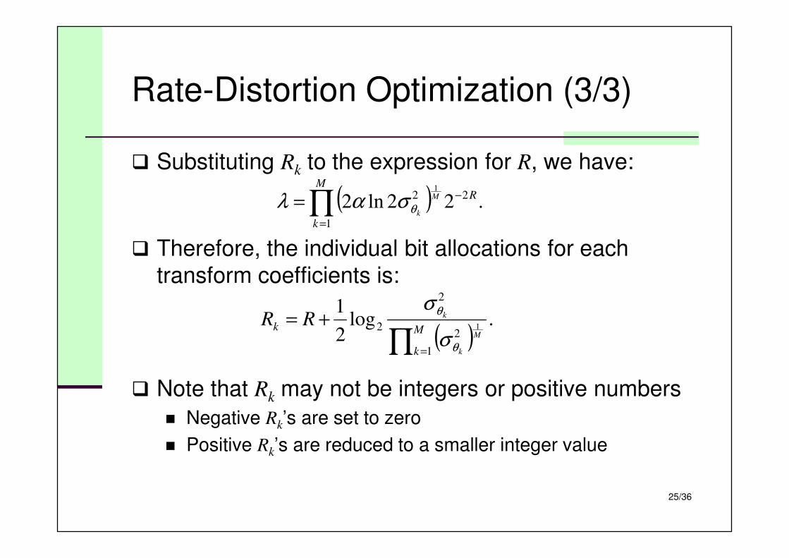
Rate-Distortion Optimization (3/3)

� Substituting Rk to the expression for R, we have:

� Therefore, the individual bit allocations for each

transform coefficients is:

� Note that Rk may not be integers or positive numbers

� Negative Rk’s are set to zero

� Positive Rk’s are reduced to a smaller integer value

( ) .22ln21

221

∏=

−=M

k

RM

kθσαλ

( ).log

2

1

1

2

2

2 1

∏ =

+=M

k

kM

k

kRR

θ

θ

σ

σ

26/36

Zonal Sampling

� Zonal sampling is a simple bit allocation algorithm:

1. Compute σθk2 for each coefficient.

2. Set Rk = 0 for all k and set Rb = MR, where Rb is the total

number of bits available for distribution.

3. Sort the variances {σθk2} Suppose σθm

2 is the maximum.

4. Increment Rm by 1, and divide σθm2 by 2.

5. Decrement Rb by 1. If Rb = 0, then stop; otherwise, go to 3.

Bit allocation map for an 8×8 transform

27/36

Threshold Coding

� Another bit allocation policy is called threshold coding

� Arrange the transform coefficients in a line

� The first coefficient is always coded

� For remaining coefficients

� If the magnitude is smaller than a threshold, it is skipped

� If the magnitude is larger than a threshold, its quantized value

and the number of skipped coefficients before it is coded

� Zigzag scan is often used for 2-D to 1-D mapping

28/36

JPEG Image Compression

� A standard defined by ISO/IEC JTC1/SC 29/WG 1

in 1992

� The official IS number is IS 10918-1, which defines the input to the decoder (a.k.a. the elementary stream), and how the decoder reconstructs the image

� The popular file format JFIF for JPEG elementary stream is defined in 10918-5

� There are several new image coding standards that

are incompatible to the old JPEG, but still bearing the

JPEG name

� Wavelet-based JPEG-2000 (IS 15444-1)

� High quality lossless/lossy JPEG-XR (IS 29199-2)

29/36

JPEG Initial Processing

� Color space RGB → YCBCR mapping

� Chroma channel 4:2:2 sub-sampling

� Level shifting: assume each pixel has p-bit, then each

pixel xi,j = xi,j – 2p–1

� Split pixels into 8×8 blocks

� If image size is not a multiple of 8, extra rows/columns are padded to achieve multiple of 8

� Padded data is discarded after decoding

30/36

JPEG 8×8 DCT Transform

� Forward DCT is applied to each 8×8 block

Level-shifting

Forward DCT

31/36

JPEG Quantization

� Midtread quantization is used; the step size for each coefficients is from an 8×8 quantization matrix Q, e.g.,

� Quantized values are called “labels.” For input

coefficient θij, we have

Qij is the step size fori,j-th transform coefficients

.5.0

+=

ij

ij

ijQ

lθ

32/36

JPEG Quantization Example

� Quantization controls the entropy of the image

� Quantization matrices reflect image quality

� A scalar number (quality factor) is often used as quantization matrix multiplier to control image quality

39.88 6.56 –2.24 1.22

–102.43 4.56 2.26 1.12

37.77 1.31 1.77 0.25

–5.67 2.24 –1.32 -0.81

16 11 10 16

12 12 14 19

14 13 16 24

14 17 22 29

θ00 Q00

2 1 0 0

–9 0 0 0

3 0 0 0

0 0 0 0

l00

299.25.016

88.395.000

0000 ==+=

+=

Ql

θ

33/36

Entropy Coding

� DC/AC coefficients are coded differently

� DCs are coded using

� Differential coding + Huffman coding

� Each DC difference is coded using a Huffman prefix plus a

fixed length suffix

� ACs are coded using

� Run-Length coding + Huffman coding

34/36

DC Difference Code Table

Differencecategory(VLC-codeas prefix)

value in each category (FLC-code as suffix)

35/36

AC RLE Code Table

� AC is zigzag scanned into a 1-D sequence

� Each non-zero coefficient is coded using a Z/C

codeword plus a sign bit S

� Z – number of zero run before the label

� C – label magnitude

� EOB is used to signal the end of each block

� ZRL is used to signal 15 consecutive zeros

36/36

JPEG Coding Example

� A good example from Wikipedia:

83,261 bytescompression ratio 2.6:1

15,138 bytescompression ratio 15:1

4,787 bytescompression ratio 46:1