This content has been downloaded from IOPscience. Please scroll down to see the full text.

Download details:

IP Address: 137.108.70.7

This content was downloaded on 03/02/2017 at 21:26

Please note that terms and conditions apply.

Imaging with polarized neutrons

View the table of contents for this issue, or go to the journal homepage for more

2009 New J. Phys. 11 043013

(http://iopscience.iop.org/1367-2630/11/4/043013)

Home Search Collections Journals About Contact us My IOPscience

You may also be interested in:

Imaging of dynamic magnetic fields with spin-polarized neutron beams

A S Tremsin, N Kardjilov, M Strobl et al.

Journal of Physics: Conference Series

S Aull, O Ebrahimi, N Karakas et al.

Comparison of Polarizers for Neutron Radiography

M Schulz, P Böni, C Franz et al.

Neutron spin manipulation optics: basic principles and possible applications

N K Pleshanov

A quantum-mechanical description of Rotating Field Spin Echo

N. Arend and W. Häuß ler

New aspects of geometric phases in experiments with polarized neutrons

S Sponar, J Klepp, K Durstberger-Rennhofer et al.

Towards a tomographic reconstruction of neutron depolarization data

Michael Schulz, Andreas Neubauer, Sergey Masalovich et al.

Powder diffraction with spin polarized neutrons

E Lelièvre-Berna, A S Wills, E Bourgeat-Lami et al.

T h e o p e n – a c c e s s j o u r n a l f o r p h y s i c s

New Journal of Physics

Imaging with polarized neutrons

Martin Dawson1, Ingo Manke1,2,4, Nikolay Kardjilov1,André Hilger1, Markus Strobl1,3 and John Banhart1,2

1 Helmholtz Centre Berlin for Materials and Energy, Germany2 Technische Universität Berlin, Germany3 Universität Heidelberg, GermanyE-mail: manke@helmholtz-berlin.de

New Journal of Physics 11 (2009) 043013 (19pp)Received 16 September 2008Published 7 April 2009Online at http://www.njp.org/doi:10.1088/1367-2630/11/4/043013

Abstract. Neutrons have zero net electrical charge and can thus penetratedeeply into matter, but their intrinsic magnetic moment makes them highlysensitive to magnetic fields. These properties have been combined withradiographic (2D) and tomographic (3D) imaging methods to provide a uniquetechnique to probe macroscopic magnetic phenomena both within and aroundbulk matter. Based on the spin-rotation of a polarized neutron beam as it passesthrough a magnetic field, this method allows the direct, real-space visualizationof magnetic field distributions. It has been used to investigate the Meissnereffect in a type I (Pb) and a type II (YBCO) superconductor, flux trapping ina type I (Pb) superconductor, and the electromagnetic field associated with adirect current flowing in a solenoid. The latter results have been compared topredictions calculated using the Biot–Savart law and have been found to agreewell.

4 Author to whom any correspondence should be addressed.

New Journal of Physics 11 (2009) 0430131367-2630/09/043013+19$30.00 © IOP Publishing Ltd and Deutsche Physikalische Gesellschaft

2

Contents

1. Introduction 22. Principles of polarized neutron imaging 23. CONRAD at the Helmholtz Centre Berlin 34. Spin filters 65. Limitations 76. Data processing/reference images 8

6.1. Separation of attenuation and spin rotation contrast . . . . . . . . . . . . . . . 86.2. Spin flipping . . . . . . . . . . . . . . . . . . . . . . . . . . . . . . . . . . . . 9

7. Results/radiography 118. Extension into three dimensions/tomography 129. Comparison between experiment and calculation 1310. Outlook/summary 17References 18

1. Introduction

Neutron imaging has proven to be successful across a broad spectrum of scientific disciplinesand industrial applications [1]–[11], providing important complementary information to thatgiven by x-rays. Their zero net electrical charge allows them to penetrate thick layers of manymaterials, yet they are sensitive to several light elements (e.g. hydrogen, boron and lithium), andare also able to differentiate isotopes of the same element. Neutrons are also highly sensitiveto magnetic fields, a property that makes them useful for investigating magnetic phenomena.Conventionally, such studies have been limited either to material surfaces and the surroundingfree space (e.g. neutron reflectometry [12] and magneto-optical effects [13]–[15]), or to bulkmagnetism (e.g. neutron spin echo, diffraction and interferometry [16]–[19]). However, recentexperimental developments at the Helmholtz Centre Berlin for Materials and Energy (formerlythe Hahn-Meitner Institute) in Germany have yielded an imaging technique that uses themagnetic interaction of spin-polarized neutrons to visualize magnetic field distributions bothin free space and within the bulk of massive samples [20]–[23].

2. Principles of polarized neutron imaging

The neutron’s sensitivity to magnetic fields lies in its intrinsic magnetic moment, Eµ (−9.66 ×

10−27J T−1); the ‘–’ indicates that the moment is always aligned anti-parallel to its associatedspin, which has a quantum number s = 1/2. Under the influence of an applied magnetic field,EB, the time-dependent behavior of the spin vector, ES, can be completely described by the

Schrödinger wave equation

d

dtES = γ

[ES(t) × EB(t)

], (1)

where γ is the gyromagnetic ratio of the neutron (−1.832 × 108 rad s−1 T−1).

New Journal of Physics 11 (2009) 043013 (http://www.njp.org/)

3

Within a field, Zeeman splitting means that there are only two possible neutron spinorientations: parallel (spin-up), and anti-parallel (spin-down), i.e. the field acts as a quantizationor polarization axis. The scalar polarization, P , is quantified as

P =N (↑) − N (↓)

N (↑) + N (↓), (2)

where N (↑) is the number of spin-up neutrons and N (↓) is the number of spin-down neutrons.This can be expressed in vector form, EP , as the average over all spin-states for the whole

beam normalized to the modulus

EP =

⟨ES⟩

1/2= 2

⟨ES⟩. (3)

It can be shown that this polarization vector behaves exactly like a classical magneticmoment [24]. In an applied magnetic field a moment experiences a torque

E0 = Eµ × EB (4)

causing it to undergo Larmor precession around the field with a frequency, ω, given by

ω = γ B, (5)

where B is the scalar magnitude of the magnetic field. For a neutron traveling along a path, s,with a velocity, v, the total precession angle, dθ , is

dθ = ωds

v, (6)

which can be expressed in terms of the neutron wavelength, λ, as

dθ =γ λm

h

∫B ds, (7)

where m is the neutron rest mass (1.675 × 10−27 kg) and h is Planck’s constant (6.626 ×

10−34 J s−1).Changes in the orientation of the moment are thus indicative of the underlying magnetic

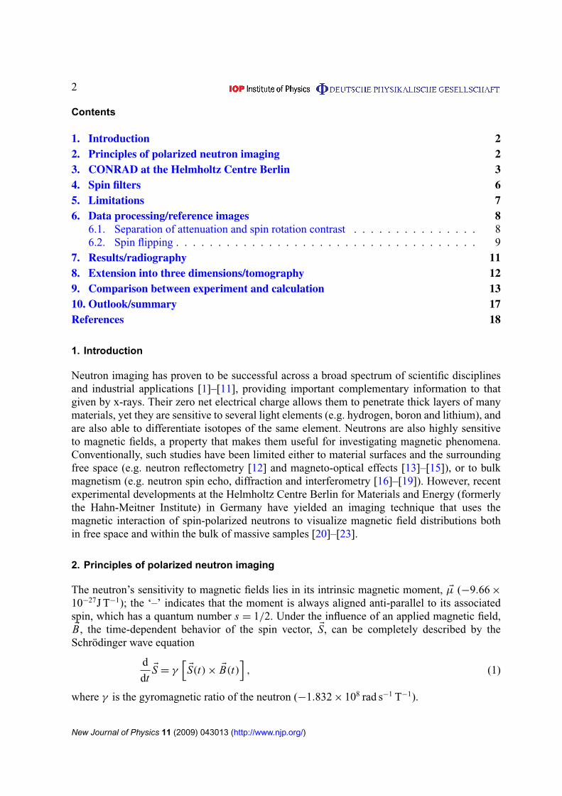
field distribution it traverses. This can be measured using a polarized neutron beam (one inwhich only one spin-state is populated) and analyzing the cumulated precession angle of thepolarization vector. If the field component perpendicular to the polarization vector is negligible,then the polarization will be preserved. If, however, the field component perpendicular to thepolarization vector is significant, then the vector will rotate, beating between states (figure 1).

Polarization analysis can be combined with standard imaging methods to visualize spatialvariations in the cumulated spin precession angle.

3. CONRAD at the Helmholtz Centre Berlin

Experiments were performed on the cold neutron radiography and tomography station(CONRAD) at the Helmholtz Centre Berlin for Materials and Energy (figure 2). CONRAD ispositioned at the end of a curved, nickel-coated neutron guide (cross section 3 × 12 cm2),which faces the cold source of the 10 MW Hahn–Meitner reactor and receives neutrons with anenergy spectrum in the range 2–10 Å (peaking at ∼3.1 Å) [25]. The instrument parameters aregiven in table 1.

New Journal of Physics 11 (2009) 043013 (http://www.njp.org/)

4

Figure 1. The orientation of the polarization axis will be preserved if it isparallel to an applied magnetic field (top), but will precess (and flip) if thereis a significant perpendicular magnetic field component.

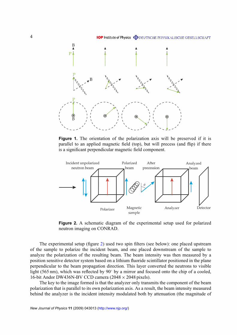
Figure 2. A schematic diagram of the experimental setup used for polarizedneutron imaging on CONRAD.

The experimental setup (figure 2) used two spin filters (see below): one placed upstreamof the sample to polarize the incident beam, and one placed downstream of the sample toanalyze the polarization of the resulting beam. The beam intensity was then measured by aposition sensitive detector system based on a lithium fluoride scintillator positioned in the planeperpendicular to the beam propagation direction. This layer converted the neutrons to visiblelight (565 nm), which was reflected by 90◦ by a mirror and focused onto the chip of a cooled,16-bit Andor DW436N-BV CCD camera (2048 × 2048 pixels).

The key to the image formed is that the analyzer only transmits the component of the beampolarization that is parallel to its own polarization axis. As a result, the beam intensity measuredbehind the analyzer is the incident intensity modulated both by attenuation (the magnitude of

New Journal of Physics 11 (2009) 043013 (http://www.njp.org/)

5

Table 1. Instrumental parameters of the two imaging positions available onCONRAD.

Typical spatial Max. neutron flux at Typical exposure Typical beam sizeL/D resolution (µm) sample (n cm−2s−1) times (s) (cm2)

Position I 70 300–500 ∼2 × 108 0.01–0.5 3 × 12Position II

3 cm aperture 167 200–400 ∼2.0 × 107 1–5 12 × 122 cm aperture 250 100–200 ∼1.0 × 107 5–15 11 × 111 cm aperture 500 50–100 ∼2.5 × 106 10–5 10 × 10

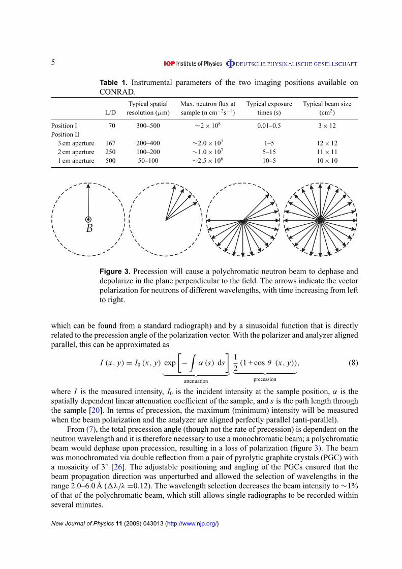
Figure 3. Precession will cause a polychromatic neutron beam to dephase anddepolarize in the plane perpendicular to the field. The arrows indicate the vectorpolarization for neutrons of different wavelengths, with time increasing from leftto right.

which can be found from a standard radiograph) and by a sinusoidal function that is directlyrelated to the precession angle of the polarization vector. With the polarizer and analyzer alignedparallel, this can be approximated as

I (x, y) = I0 (x, y) exp[−

∫α (s) ds

]︸ ︷︷ ︸

attenuation

1

2(1 + cos θ (x, y))︸ ︷︷ ︸

precession

, (8)

where I is the measured intensity, I0 is the incident intensity at the sample position, α is thespatially dependent linear attenuation coefficient of the sample, and s is the path length throughthe sample [20]. In terms of precession, the maximum (minimum) intensity will be measuredwhen the beam polarization and the analyzer are aligned perfectly parallel (anti-parallel).

From (7), the total precession angle (though not the rate of precession) is dependent on theneutron wavelength and it is therefore necessary to use a monochromatic beam; a polychromaticbeam would dephase upon precession, resulting in a loss of polarization (figure 3). The beamwas monochromated via double reflection from a pair of pyrolytic graphite crystals (PGC) witha mosaicity of 3◦ [26]. The adjustable positioning and angling of the PGCs ensured that thebeam propagation direction was unperturbed and allowed the selection of wavelengths in therange 2.0–6.0 Å (1λ/λ =0.12). The wavelength selection decreases the beam intensity to ∼1%of that of the polychromatic beam, which still allows single radiographs to be recorded withinseveral minutes.

New Journal of Physics 11 (2009) 043013 (http://www.njp.org/)

6

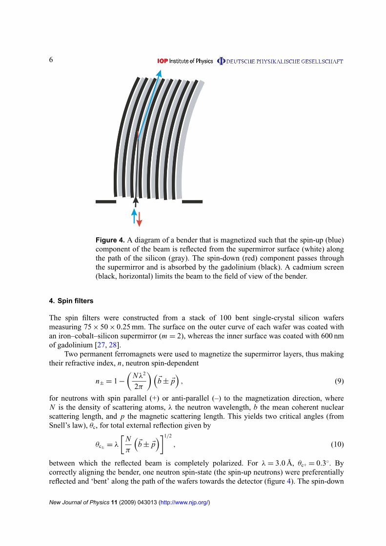
Figure 4. A diagram of a bender that is magnetized such that the spin-up (blue)component of the beam is reflected from the supermirror surface (white) alongthe path of the silicon (gray). The spin-down (red) component passes throughthe supermirror and is absorbed by the gadolinium (black). A cadmium screen(black, horizontal) limits the beam to the field of view of the bender.

4. Spin filters

The spin filters were constructed from a stack of 100 bent single-crystal silicon wafersmeasuring 75 × 50 × 0.25 mm. The surface on the outer curve of each wafer was coated withan iron–cobalt–silicon supermirror (m = 2), whereas the inner surface was coated with 600 nmof gadolinium [27, 28].

Two permanent ferromagnets were used to magnetize the supermirror layers, thus makingtheir refractive index, n, neutron spin-dependent

n± = 1 −

(Nλ2

2π

) (Eb ± Ep

), (9)

for neutrons with spin parallel (+) or anti-parallel (–) to the magnetization direction, whereN is the density of scattering atoms, λ the neutron wavelength, b the mean coherent nuclearscattering length, and p the magnetic scattering length. This yields two critical angles (fromSnell’s law), θc, for total external reflection given by

θc±= λ

[N

π

(Eb ± Ep

)]1/2

, (10)

between which the reflected beam is completely polarized. For λ = 3.0 Å, θc+ = 0.3◦. Bycorrectly aligning the bender, one neutron spin-state (the spin-up neutrons) were preferentiallyreflected and ‘bent’ along the path of the wafers towards the detector (figure 4). The spin-down

New Journal of Physics 11 (2009) 043013 (http://www.njp.org/)

7

Figure 5. A radiograph showing the vertical striping inhomogeneities producedby the structure of a bender. The field of view is 1.5 × 4.5 cm.

neutrons passed through the supermirror and were absorbed by the gadolinium layer (i.e. therewas no straight-through beam). The typical polarization achieved with such a bender is 95%.

A cadmium screen with a window 1 × 4 cm was placed in front of each bender (polarizerand analyzer) in order to prevent neutrons that had not passed through both benders fromreaching the detector. Objects larger than this window could still be imaged by scanning thesample and recombining images from multiple positions.

Some disadvantages of using benders are that beam attenuation caused by their physicalstructure produces vertical striping inhomogeneities in the beam intensity profile (figure 5), andthe polarization produced is non-uniform across the beam (the beam polarization received byneighboring pixels can vary by 5%). These factors can be corrected (by normalization), but theyhave an impact on the potential quality of the data and create inaccuracies in the recombinedimages of larger samples.

5. Limitations

The experimental arrangement outlined above has some limitations. First of all, it can onlybe applied reliably to magnetic fields below a certain strength, as the beam’s imperfectmonochromaticity means that multiple precessions in regions where the field is too strongwill lead to multiple, non-distinguishable rotations and, eventually, dephasing. If the neutronsdephase completely then the beam will no longer be polarized and it will not be possible toresolve any magnetic effects. The problem of dephasing could be overcome by improving thebeam monochromaticity or using a spin-echo setup [29] to counteract the multiple precessions.

Secondly, the uniaxial polarization analysis means that measurement of the exact vectorfield distribution is not straight forward, since only the scalar polarization is measured.Information about the polarization vector in the plane perpendicular to the polarization axis

New Journal of Physics 11 (2009) 043013 (http://www.njp.org/)

8

is lost; in general, a precession of φ is indistinguishable from a rotation of nπ ± φ (n = 2, 4,6, . . . ) around the same axis. In order to recover the three-dimensional (3D) vector polarization,it is necessary to measure the scalar polarization in three mutually orthogonal directions, e.g. byusing spin flippers. However, a complex 3D vector field will produce a spin rotation that cannotbe easily correlated to the vector field from which it originated (see below).

It should be noted that the limitation of field strength with respect to multiple precessionsand dephasing depends on both the field strength and the length of the path (cf (7)); as thepath length is reduced, stronger fields can be tolerated. For a polarized monochromatic beamwith 1λ/λ = 0.1 traversing a uniform field-oriented perpendicular to the beam propagationdirection, after ten complete precessions the spins of the lowest energy neutrons will be 2π outof phase with those of the highest energy neutrons (i.e. the beam would be unpolarized). For apath length of 1 cm, this would occur for a field of ∼50 mT.

Finally, the experimental setup includes an inherent short-coming in that, for parallel beamgeometry with a finite beam divergence, the best spatial resolution is attained with a minimumdistance between the sample and the detector. Clearly, the necessity for the analyzer betweenthe sample and the detector increases the separation. This is compounded by the fact that, whenimaging samples that have/require strong magnetic fields, the sample–analyzer distance mustbe increased further in order to limit the effect of the field on the working of the analyzer. Theincreased separation leads to a reduction in spatial resolution and losses in the image quality.

6. Data processing/reference images

6.1. Separation of attenuation and spin rotation contrast

Radiographic images require normalization to a reference image in order to correct forinstrumental inhomogeneities (e.g. in the intensity profile across the beam). The reference isusually an open beam image (i.e. one in which no sample is present), but for polarized neutronimaging it is sometimes more useful to use an image of the sample in the absence of anymagnetic field, i.e. by switching the field off (in the case of electromagnetic or externally appliedfields). Since attenuation and spin rotation are mutually independent (cf (8)), such a referenceimage allows them to be separated from one another; both beam inhomogeneities and sampleattenuation are normalized, resulting in an image that contains only magnetic effects. This isparticularly useful when attenuation is the dominant effect and subtle magnetic effects wouldotherwise be overwhelmed. Note that this method is not possible if the magnetic field cannot beswitched off (naturally magnetized materials for example); in such cases, the reference image isan image containing the polarizer and analyzer (this corrects for inherent beam inhomogeneitiesand inhomogeneities introduced by the polarization equipment).

This is demonstrated in figure 6, which shows a pellet of YBa2Cu3O7 (YBCO), a typeII superconductor, cooled below its critical temperature (Tc = 90 K) in the presence of ahomogeneous 0.1 mT field. As a consequence of the Meissner effect, the magnetic field isexpelled in the superconducting state (see figure 6(a)). Due to neutron absorption in the pellet,it is difficult to differentiate between attenuation and magnetic signals in the raw imagesmeasured at 100 and 20 K (figure 6(b)). However, normalization of these images to an imagemeasured at 100 K in the absence of an applied magnetic field allows the magnetic signal to beviewed independently (figure 6(c)). At 100 K the magnetic field is distributed homogeneously(the signal in the image is uniform). At 20 K strong inhomogeneities caused by the expulsion of

New Journal of Physics 11 (2009) 043013 (http://www.njp.org/)

9

Figure 6. Images of the field associated with the Meissner effect in asuperconducting YBCO pellet ( ∅2 cm) above and below the critical temperature(Tc = 90 K), showing (a) schematic diagrams, (b) raw (unnormalized) radio-graphs, and (c) radiographs normalized to a reference image. The reference wasan image of the sample in zero field at 100 K. The arrow indicates a region whereexpulsion of the field is incomplete.

the field from the pellet can be seen. Three regions can be distinguished. For neutrons passingthrough the unperturbed field, the precession angle remains constant; the measured intensityhere is uniform (A in figure 6). For neutrons passing through the pellet, the field is reduced andthe precession angle is smaller than in the unperturbed region; the measured intensity here ishigher than in the unperturbed region (cf (8)) (B in figure 6). For neutrons passing through theregions of stronger magnetic field (above and below the pellet in figure 6(a)), the precessionangle is larger than in the unperturbed region; the measured intensity here is lower than in theunperturbed region (cf (8)) (C in figure 6). The latter point applies also to a defect running acrossthe pellet in which some of the expelled magnetic field becomes trapped.

6.2. Spin flipping

The contrast of the magnetic field in an image can be switched by using (for example) a spinflipper to rotate the beam polarization incident at the sample position by π , this is equivalent tothe polarization and analysis axes being aligned anti-parallel. In this case, the intensity measuredbehind the analyzer is given approximately by

I (x, y) = I0 (x, y) exp[−

∫α (s) ds

]︸ ︷︷ ︸

attenuation

1

2(1 − cos θ (x, y))︸ ︷︷ ︸

precession

(11)

New Journal of Physics 11 (2009) 043013 (http://www.njp.org/)

10

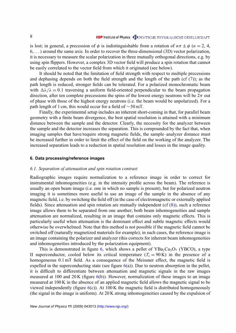
Figure 7. Radiographs of the magnetic field associated with the Meissnereffect in a superconducting lead cylinder (Tc = 7.2 K), ∅1 × 3 cm, showing thesituation (a) and (b) with, and (c) without a π -flipper positioned between thepolarizer and the sample. As a comparison, (d) is the negative image of (b).The red, dashed/blue, solid box indicates the approximate position of the leadcylinder/the steel fixture holding the cylinder in place. The arrows indicateequivalent positions and are intended as a guide to the eye.

(cf (8)). This is demonstrated in figure 7, which shows the magnetic field distributioninside and around a lead cylinder, a type I superconductor (Tc = 7.2 K) (cf figures 9, 11and 12). A homogeneous 10 mT magnetic field was applied parallel to the cylinder axis andperpendicular to the beam polarization axis and images were recorded above and below thecritical temperature. Above Tc the field permeates the lead (figure 7(a)), but below Tc the fieldis largely expelled (figure 7(b)) due to the Meissner effect, resulting in disturbances in thefield in the vicinity of the cylinder.

Figure 7(c) is measured with the same arrangement as figure 7(b), but with the beampolarization flipped by π before interaction with the sample. The image recorded without theπ -flip is approximately the negative of that recorded with the π -flip (i.e. dark becomes brightand vice versa, see red arrows). However, the regions in figure 7(b) where attenuation isdominant remain constant (i.e. the steel fixture holding the sample in place is dark in bothcases (blue solid box)). For comparison, an actual negative image of figure 7(a) is shown infigure 7(d). In regions where magnetic effects dominate (i.e. in free space and inside the lead)

New Journal of Physics 11 (2009) 043013 (http://www.njp.org/)

11

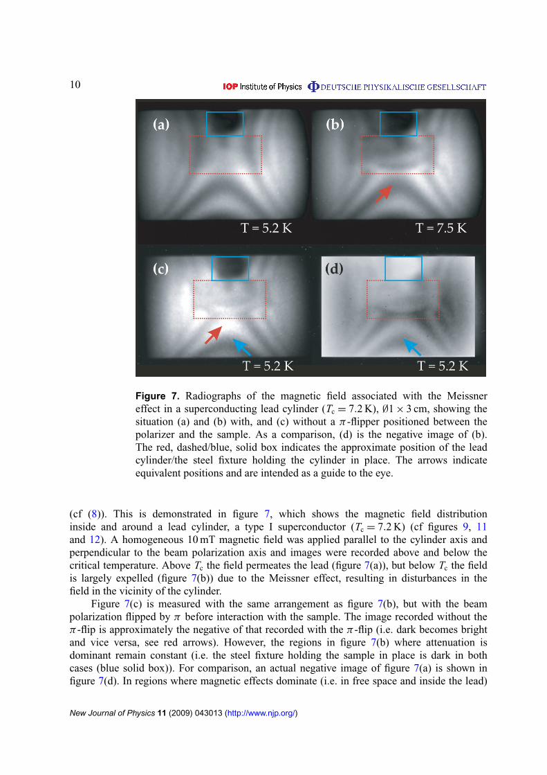
Figure 8. Radiograph of the magnetic field surrounding a pair of ring-shapeddipole magnets, oriented horizontally in the plane of the paper, separated by asheet of aluminum (edges indicated by arrows.). The field of view is 13.8 ×

11.3 cm and is a composite of images measured at three different positions.([20], supplementary information.)

figures 7(c) and 8(d) correspond very well (blue arrows), but the contrast is switched in regionswhere attenuation dominates.

7. Results/radiography

The utility of this technique has already been demonstrated with a variety of magnetic systems.Figure 8 shows a radiographic image of a pair of ring-shaped magnets (the dipoles are orientedhorizontally in the plane of the paper) separated by a piece of aluminum. The magnetic field isvisible both in free space and within the bulk of the aluminum spacer (arrows). The strength ofthe magnetic field around the magnet diminishes (approximately) with the inverse of the squareof the distance from the magnets. As a result, the magnitude of the total neutron precessionalso declines, resulting in a series of maxima and minima in intensity, whose period increaseswith distance (cf (8)). The image shown is approximately 13.8 × 11.3 cm and is a composite ofimages measured at three different positions (due to the limited field of view of the benders).Imperfect screening of the magnetic sample meant that the magnetic field interfered with thepolarizing properties of the analyzing bender. Thus, as the relative positions of the sample andanalyzer were adjusted for each image, the measured polarization changed also. Consequently,the three individual images do not align exactly.

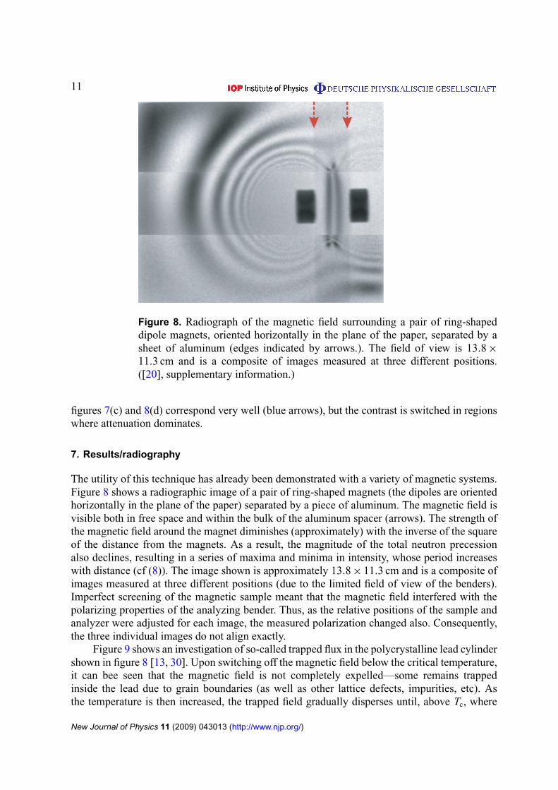
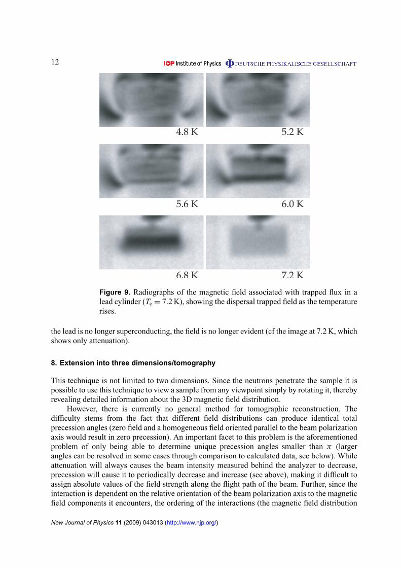
Figure 9 shows an investigation of so-called trapped flux in the polycrystalline lead cylindershown in figure 8 [13, 30]. Upon switching off the magnetic field below the critical temperature,it can bee seen that the magnetic field is not completely expelled—some remains trappedinside the lead due to grain boundaries (as well as other lattice defects, impurities, etc). Asthe temperature is then increased, the trapped field gradually disperses until, above Tc, where

New Journal of Physics 11 (2009) 043013 (http://www.njp.org/)

12

Figure 9. Radiographs of the magnetic field associated with trapped flux in alead cylinder (Tc = 7.2 K), showing the dispersal trapped field as the temperaturerises.

the lead is no longer superconducting, the field is no longer evident (cf the image at 7.2 K, whichshows only attenuation).

8. Extension into three dimensions/tomography

This technique is not limited to two dimensions. Since the neutrons penetrate the sample it ispossible to use this technique to view a sample from any viewpoint simply by rotating it, therebyrevealing detailed information about the 3D magnetic field distribution.

However, there is currently no general method for tomographic reconstruction. Thedifficulty stems from the fact that different field distributions can produce identical totalprecession angles (zero field and a homogeneous field oriented parallel to the beam polarizationaxis would result in zero precession). An important facet to this problem is the aforementionedproblem of only being able to determine unique precession angles smaller than π (largerangles can be resolved in some cases through comparison to calculated data, see below). Whileattenuation will always causes the beam intensity measured behind the analyzer to decrease,precession will cause it to periodically decrease and increase (see above), making it difficult toassign absolute values of the field strength along the flight path of the beam. Further, since theinteraction is dependent on the relative orientation of the beam polarization axis to the magneticfield components it encounters, the ordering of the interactions (the magnetic field distribution

New Journal of Physics 11 (2009) 043013 (http://www.njp.org/)

13

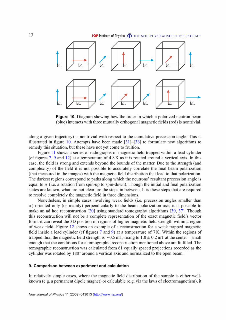
Figure 10. Diagram showing how the order in which a polarized neutron beam(blue) interacts with three mutually orthogonal magnetic fields (red) is nontrivial.

along a given trajectory) is nontrivial with respect to the cumulative precession angle. This isillustrated in figure 10. Attempts have been made [31]–[36] to formulate new algorithms toremedy this situation, but these have not yet come to fruition.

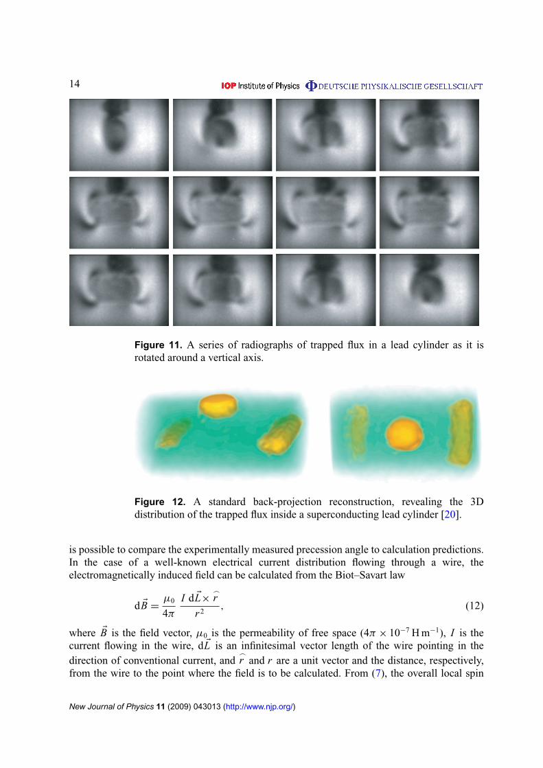
Figure 11 shows a series of radiographs of magnetic field trapped within a lead cylinder(cf figures 7, 9 and 12) at a temperature of 4.8 K as it is rotated around a vertical axis. In thiscase, the field is strong and extends beyond the bounds of the matter. Due to the strength (andcomplexity) of the field it is not possible to accurately correlate the final beam polarization(that measured in the images) with the magnetic field distribution that lead to that polarization.The darkest regions correspond to paths along which the neutrons’ resultant precession angle isequal to π (i.e. a rotation from spin-up to spin-down). Though the initial and final polarizationstates are known, what are not clear are the steps in between. It is these steps that are requiredto resolve completely the magnetic field in three dimensions.

Nonetheless, in simple cases involving weak fields (i.e. precession angles smaller thanπ ) oriented only (or mainly) perpendicularly to the beam polarization axis it is possible tomake an ad hoc reconstruction [20] using standard tomography algorithms [30, 37]. Thoughthis reconstruction will not be a complete representation of the exact magnetic field’s vectorform, it can reveal the 3D position of regions of higher magnetic field strength within a regionof weak field. Figure 12 shows an example of a reconstruction for a weak trapped magneticfield inside a lead cylinder (cf figures 7 and 9) at a temperature of 7 K. Within the regions oftrapped flux, the magnetic field strength is ∼0.5 mT, rising to 1.0 ± 0.2 mT at the center—smallenough that the conditions for a tomographic reconstruction mentioned above are fulfilled. Thetomographic reconstruction was calculated from 61 equally spaced projections recorded as thecylinder was rotated by 180◦ around a vertical axis and normalized to the open beam.

9. Comparison between experiment and calculation

In relatively simple cases, where the magnetic field distribution of the sample is either well-known (e.g. a permanent dipole magnet) or calculable (e.g. via the laws of electromagnetism), it

New Journal of Physics 11 (2009) 043013 (http://www.njp.org/)

14

Figure 11. A series of radiographs of trapped flux in a lead cylinder as it isrotated around a vertical axis.

Figure 12. A standard back-projection reconstruction, revealing the 3Ddistribution of the trapped flux inside a superconducting lead cylinder [20].

is possible to compare the experimentally measured precession angle to calculation predictions.In the case of a well-known electrical current distribution flowing through a wire, theelectromagnetically induced field can be calculated from the Biot–Savart law

d EB =µ0

4π

I d EL×_r

r 2, (12)

where EB is the field vector, µ0 is the permeability of free space (4π × 10−7 H m−1), I is thecurrent flowing in the wire, d EL is an infinitesimal vector length of the wire pointing in thedirection of conventional current, and

_r and r are a unit vector and the distance, respectively,

from the wire to the point where the field is to be calculated. From (7), the overall local spin

New Journal of Physics 11 (2009) 043013 (http://www.njp.org/)

15

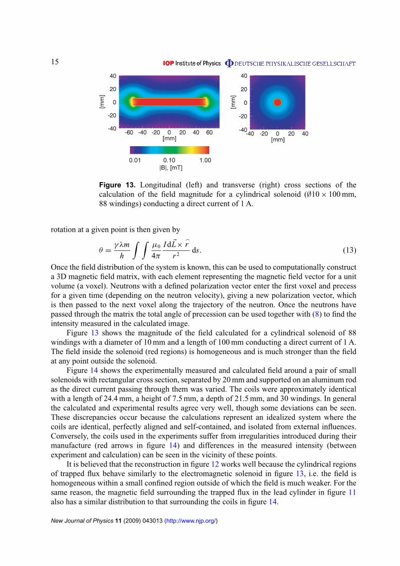
Figure 13. Longitudinal (left) and transverse (right) cross sections of thecalculation of the field magnitude for a cylindrical solenoid (∅10 × 100 mm,88 windings) conducting a direct current of 1 A.

rotation at a given point is then given by

θ =γ λm

h

∫ ∫µ0

4π

I d EL×_r

r 2ds. (13)

Once the field distribution of the system is known, this can be used to computationally constructa 3D magnetic field matrix, with each element representing the magnetic field vector for a unitvolume (a voxel). Neutrons with a defined polarization vector enter the first voxel and precessfor a given time (depending on the neutron velocity), giving a new polarization vector, whichis then passed to the next voxel along the trajectory of the neutron. Once the neutrons havepassed through the matrix the total angle of precession can be used together with (8) to find theintensity measured in the calculated image.

Figure 13 shows the magnitude of the field calculated for a cylindrical solenoid of 88windings with a diameter of 10 mm and a length of 100 mm conducting a direct current of 1 A.The field inside the solenoid (red regions) is homogeneous and is much stronger than the fieldat any point outside the solenoid.

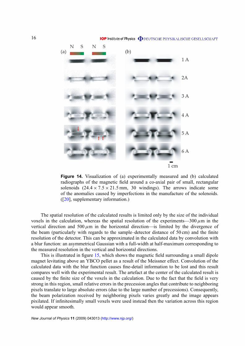
Figure 14 shows the experimentally measured and calculated field around a pair of smallsolenoids with rectangular cross section, separated by 20 mm and supported on an aluminum rodas the direct current passing through them was varied. The coils were approximately identicalwith a length of 24.4 mm, a height of 7.5 mm, a depth of 21.5 mm, and 30 windings. In generalthe calculated and experimental results agree very well, though some deviations can be seen.These discrepancies occur because the calculations represent an idealized system where thecoils are identical, perfectly aligned and self-contained, and isolated from external influences.Conversely, the coils used in the experiments suffer from irregularities introduced during theirmanufacture (red arrows in figure 14) and differences in the measured intensity (betweenexperiment and calculation) can be seen in the vicinity of these points.

It is believed that the reconstruction in figure 12 works well because the cylindrical regionsof trapped flux behave similarly to the electromagnetic solenoid in figure 13, i.e. the field ishomogeneous within a small confined region outside of which the field is much weaker. For thesame reason, the magnetic field surrounding the trapped flux in the lead cylinder in figure 11also has a similar distribution to that surrounding the coils in figure 14.

New Journal of Physics 11 (2009) 043013 (http://www.njp.org/)

16

Figure 14. Visualization of (a) experimentally measured and (b) calculatedradiographs of the magnetic field around a co-axial pair of small, rectangularsolenoids (24.4 × 7.5 × 21.5 mm, 30 windings). The arrows indicate someof the anomalies caused by imperfections in the manufacture of the solenoids.([20], supplementary information.)

The spatial resolution of the calculated results is limited only by the size of the individualvoxels in the calculation, whereas the spatial resolution of the experiments—300 µm in thevertical direction and 500 µm in the horizontal direction—is limited by the divergence ofthe beam (particularly with regards to the sample–detector distance of 50 cm) and the finiteresolution of the detector. This can be approximated in the calculated data by convolution witha blur function: an asymmetrical Gaussian with a full-width at half-maximum corresponding tothe measured resolution in the vertical and horizontal directions.

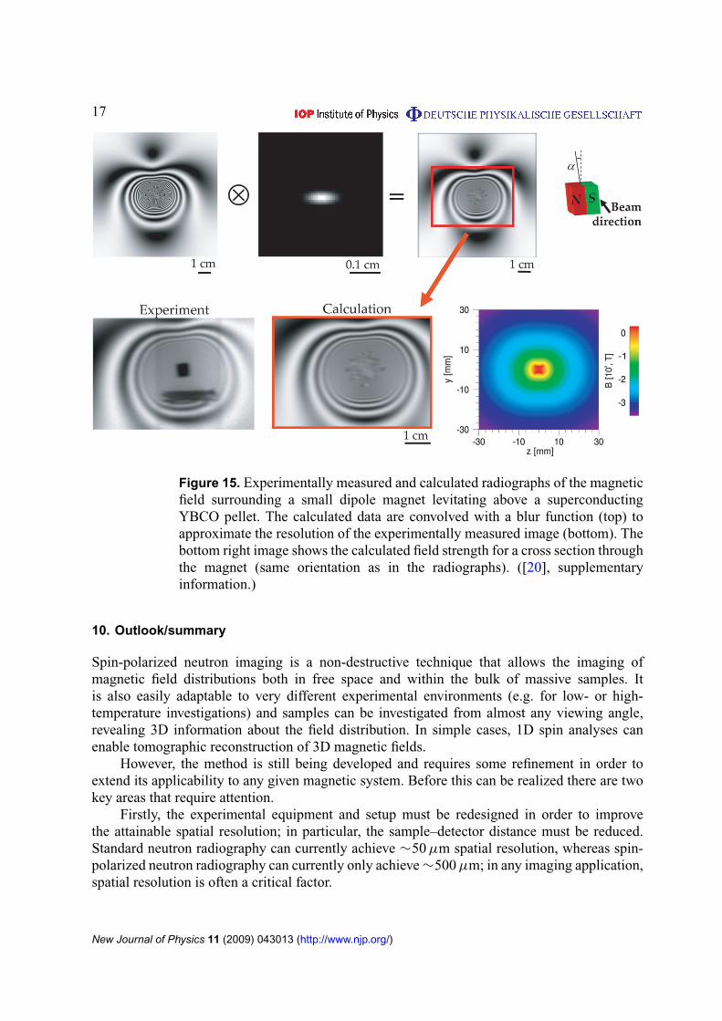
This is illustrated in figure 15, which shows the magnetic field surrounding a small dipolemagnet levitating above an YBCO pellet as a result of the Meissner effect. Convolution of thecalculated data with the blur function causes fine-detail information to be lost and this resultcompares well with the experimental result. The artefact at the center of the calculated result iscaused by the finite size of the voxels in the calculation. Due to the fact that the field is verystrong in this region, small relative errors in the precession angles that contribute to neighboringpixels translate to large absolute errors (due to the large number of precessions). Consequently,the beam polarization received by neighboring pixels varies greatly and the image appearspixilated. If infinitesimally small voxels were used instead then the variation across this regionwould appear smooth.

New Journal of Physics 11 (2009) 043013 (http://www.njp.org/)

17

Figure 15. Experimentally measured and calculated radiographs of the magneticfield surrounding a small dipole magnet levitating above a superconductingYBCO pellet. The calculated data are convolved with a blur function (top) toapproximate the resolution of the experimentally measured image (bottom). Thebottom right image shows the calculated field strength for a cross section throughthe magnet (same orientation as in the radiographs). ([20], supplementaryinformation.)

10. Outlook/summary

Spin-polarized neutron imaging is a non-destructive technique that allows the imaging ofmagnetic field distributions both in free space and within the bulk of massive samples. Itis also easily adaptable to very different experimental environments (e.g. for low- or high-temperature investigations) and samples can be investigated from almost any viewing angle,revealing 3D information about the field distribution. In simple cases, 1D spin analyses canenable tomographic reconstruction of 3D magnetic fields.

However, the method is still being developed and requires some refinement in order toextend its applicability to any given magnetic system. Before this can be realized there are twokey areas that require attention.

Firstly, the experimental equipment and setup must be redesigned in order to improvethe attainable spatial resolution; in particular, the sample–detector distance must be reduced.Standard neutron radiography can currently achieve ∼50 µm spatial resolution, whereas spin-polarized neutron radiography can currently only achieve ∼500 µm; in any imaging application,spatial resolution is often a critical factor.

New Journal of Physics 11 (2009) 043013 (http://www.njp.org/)

18

Secondly, and more importantly, is the conception of new algorithms that allow thetranslation of projections recorded at different viewing angles into 3D magnetic vector fieldmatrices.

Future applications of spin-polarized neutron imaging will include further investigationsof many effects in bulk magnetism. The most important of these could be magnetic domaindistributions in crystals, and magnetoelastic and magnetostrictive stress and strains.

References

[1] Lehmann E and Kardjilov N 2008 Advanced Tomographic Methods in Materials Research and Engineeringed J Banhart (New York: Oxford University Press) pp 375–406

[2] Herman G T 1980 Image Reconstruction from Projections: The Fundamentals of Computerized Tomography(New York: Academic)

[3] Schillinger B, Lehmann E and Vontobel P 2000 3D neutron computed tomography: requirements andapplications Physica B 276 59–62

[4] Kardjilov N, Hilger A, Manke I, Strobl M and Banhart J 2005 Industrial applications at the new cold neutronradiography and tomography facility of the HMI Nucl. Instrum. Methods A 542 16–21

[5] Allman B E, McMahon P J, Nugent K A, Paganin D, Jacobson D L, Arif M and Werner S A 2000 Phaseradiography with neutrons Nature 408 158–9

[6] Pfeiffer F, Grünzweig C, Bunk O, Frei G, Lehmann E and David C 2006 Neutron phase imaging andtomography Phys. Rev. Lett. 96 215505

[7] Manke I, Hartnig Ch, Grünerbel M, Kaczerowski J, Lehnert W, Kardjilov N, Hilger A, Banhart J, TreimerW and Strobl M 2007 Quasi-in situ neutron tomography on polymer electrolyte membrane fuel cell stacksAppl. Phys. Lett. 90 184101

[8] Strobl M, Grünzweig C, Hilger A, Manke I, Kardjilov N, David C and Pfeiffer F 2008 Neutron dark-fieldtomography Phys. Rev. Lett. 101 123902

[9] Hickner M A, Siegel N P, Chen K S, Hussey D S, Jacobson D L and Arif M 2008 In situ high-resolutionneutron radiography of cross-sectional liquid water profiles in proton exchange membrane fuel cellsJ. Electrochem. Soc. 155 B427–34

[10] Boillat P, Kramer D, Seyfang B C, Frei G, Lehmann E, Scherer G G, Wokaun A, Ichikawa Y, Tasaki Y andShinohara K 2008 In situ observation of the water distribution across a PEFC using high resultion neutronradiography Electrochem. Commun. 10 546–50

[11] Manke I, Hartnig Ch, Kardjilov N, Messerschmidt M, Hilger A, Strobl M, Lehnert W and Banhart J2008 Characterization of water exchange and two-phase flow in porous gas diffusion materials byhydrogen–deuterium contrast neutron radiography Appl. Phys. Lett. 92 244101

[12] Ankner J F and Felcher G P 1999 Polarized-neutron reflectometry J. Magn. Magn. Mater. 200 741–54[13] Gammel P and Bishop D 1998 Fingerprinting vortices with smoke Science 279 410–1[14] Jooss Ch, Albrecht J, Kuhn H, Leonhardt S and Kronmüller H 2002 Magneto-optical studies of current

distributions in high-Tc superconductors Rep. Prog. Phys. 65 651–788[15] Johansen T H and Shantsev D V 2004 Magneto-Optical Imaging (Dordrecht: Springer)[16] Mezei F 1972 Neutron spin echo: a new concept in polarized thermal neutron techniques Z. Phys. 255 146–60[17] Brandstätter G, Weber H W, Chattopadhyay T, Cubitt R, Fischer H, Wylie M, Emel’chenko G A and

Wiedenmann A 1997 Neutron diffraction by the flux line lattice in YBa2Cu3O7−δ single crystals J. Appl.Crystallogr. 30 571–4

[18] Schlenker M, Bauspiess W, Graeff W, Bonse U and Rauch H 1980 Imaging of feromagnitic domains byneutron interferometry J. Magn. Magn. Mater. 15–18 1507–9

[19] Rauch H and Werner S 2000 Neutron Interferometry (Oxford: Oxford University Press)[20] Kardjilov N, Manke I, Strobl M, Hilger A, Treimer W, Meissner M, Krist T and Banhart J 2008

Three-dimensional imaging of magnetic field with polarized neutrons Nat. Phys. 4 399–403

New Journal of Physics 11 (2009) 043013 (http://www.njp.org/)

19

[21] Kardjilov N, Manke I, Hilger A, Dawson M and Banhart J 2008 Tech spotlight: imaging with magneticneutrons Adv. Mater. Process. 166 43–4

[22] Manke I, Kardjilov N, Strobl M, Hilger A and Banhart J 2008 Investigation of the skin effect in the bulk ofelectrical conductors with spin-polarized neutron radiography J. Appl. Phys. 104 076109

[23] Strobl M, Treimer W, Walter P, Keil S and Manke I 2007 Magnetic field induced differential neutron phasecontrast imaging Appl. Phys. Lett. 91 254104

[24] Mezei F (ed) 1980 Neutron Spin Echo Lecture Notes in Physics vol 128 (Berlin: Springer)[25] Hilger A, Kardjilov N, Strobl M, Treimer W and Banhart J 2006 The new cold neutron radiography and

tomography instrument CONRAD at HMI Berlin Physica B 385–386 1213–5[26] Treimer W, Strobl M, Kardjilov N, Hilger A and Manke I 2006 Wavelength tunable device for neutron

radiography and tomography Appl. Phys. Lett. 89 203504[27] Krist T, Kennedy S J, Hick T J and Mezei F 1998 New compact neutron polarizer Physica B 241–243 82–5[28] Krist T, Peters J, Shimizu H M, Suzuki J and Oku T 2005 Transmission bender for polarizing neutrons Physica

B 356 197–200[29] Piegsa F M, van den Brandt B, Hautle P and Konter J A 2008 Neutron spin phase imaging Nucl. Instrum.

Methods A 586 15–7[30] Banhart J (ed) 2008 Advanced Tomographic Methods in Materials Research and Engineering (Oxford:

Oxford University Press)[31] Hochhold M, Leeb H and Badurek G 1996 Tensorial neutron tomography: a first approach J. Magn. Magn.

Mater. 157–158 575–6[32] Badurek G, Hochhold M and Leeb H 1997 Neutron magnetic tomography—a novel technique Physica

B 234–236 1171–3[33] Badurek G, Hochhold M, Leeb H, Buchelt R and Korinek F 1997 A proposal to visualize magnetic domains

within bulk materials Physica B 241–243 1207–9[34] Leeb H, Hochhold M, Badurek G, Buchelt R J and Schricker A 1998 Neutron magnetic tomography:

a feasibility study Aust. J. Phys. 51 401–13[35] Leeb H, Szeywerth R, Jericha E and Badurek G 2005 Towards manageable magnetic field retrieval in bulk

materials Physica B 356 187–91[36] Jericha E, Szeywerth R, Leeb H and Badurek G 2007 Reconstruction techniques for tensorial neutron

tomography Physica B 397 159–61[37] Herman G T 1980 Image Reconstruction from Projections: The Fundamentals of Computerized Tomography

(New York: Academic)

New Journal of Physics 11 (2009) 043013 (http://www.njp.org/)