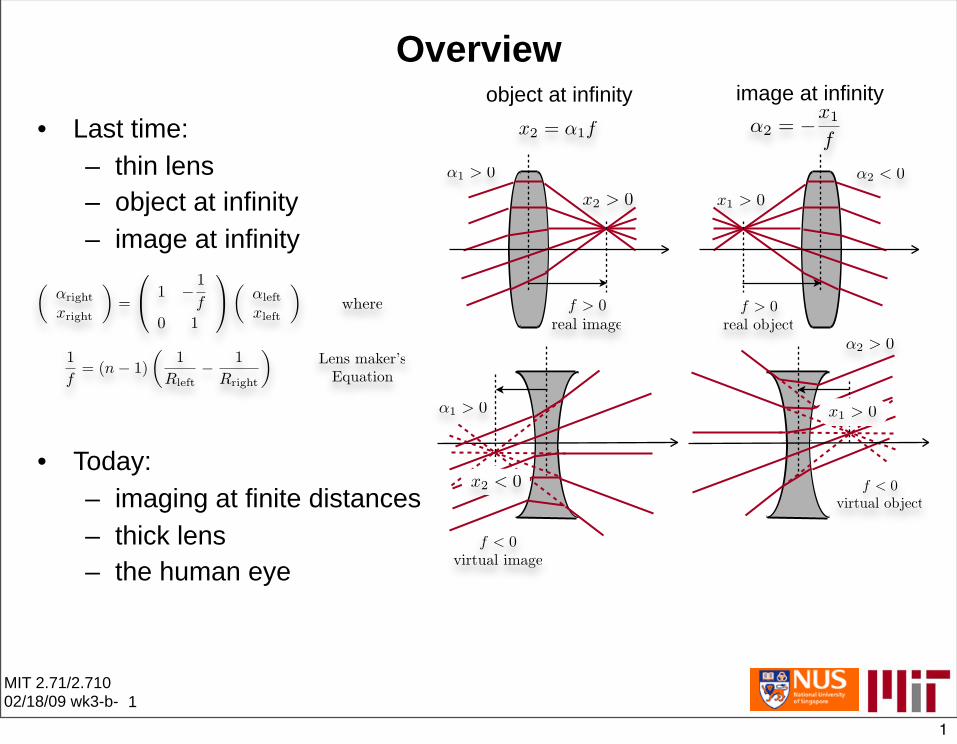
Overview object at infinity image at infinity

• Last time: – thin lens – object at infinity – image at infinity

• Today: – imaging at finite distances – thick lens – the human eye

MIT 2.71/2.710 02/18/09 wk3-b- 1

1

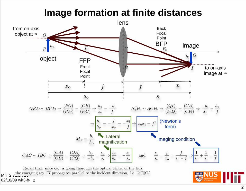
Image formation at finite distances

MIT 2.71/2.710 02/18/09 wk3-b- 2

object

image

FFP Front Focal Point

Back Focal Point BFP

lens from on-axis object at ∞

to on-axis image at ∞

Lateral magnification Imaging condition

(Newton’s form)

2

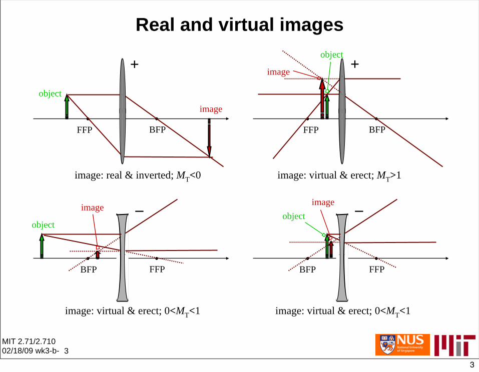
Real and virtual images

BFP

object

image

FFP BFP

object

image

FFP

+ +

image: real & inverted; MT<0 image: virtual & erect; MT>1

FFPBFP

object

image –

FFPBFP

object image –

image: virtual & erect; 0<MT<1 image: virtual & erect; 0<MT<1

MIT 2.71/2.710 02/18/09 wk3-b- 3

3

5

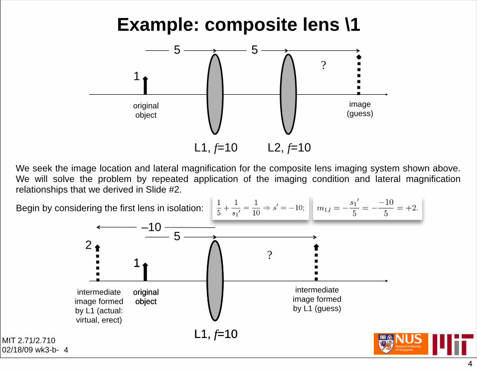
Example: composite lens \1

L1, f=10 L2, f=10

5 5

original object

image

? 1

(guess)

We seek the image location and lateral magnification for the composite lens imaging system shown above. We will solve the problem by repeated application of the imaging condition and lateral magnification relationships that we derived in Slide #2.

MIT 2.71/2.710 02/18/09 wk3-b- 4

Begin by considering the first lens in isolation:

L1, f=10L1,

original object

?1

intermediate image formed by L1 (guess)

5

original

f=10

object

12

intermediate image formed by L1 (actual: virtual, erect)

–10

4

L1, f=10 L2, f=10

5 5

originalobject

?1

image (guess)

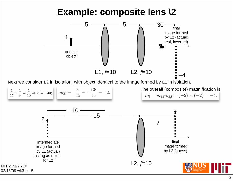
Example: composite lens \2 5 5

original object

1

30final

image formed by L2 (actual: real, inverted)

L1, f=10 L2, f=10 –4 Next we consider L2 in isolation, with object identical to the image formed by L1 in isolation.

The overall (composite) magnification is

2 ?

final image formed intermediate

image formed by L1 (actual) by L2 (guess)

acting as object for L2

–10 15

L2, f=10MIT 2.71/2.710 02/18/09 wk3-b- 5

5

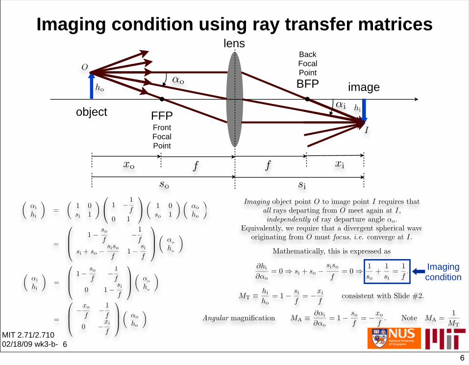
Imaging condition using ray transfer matrices lens

MIT 2.71/2.710 02/18/09 wk3-b- 6

object

image

FFP Front Focal Point

Back Focal Point BFP

Imaging condition

6

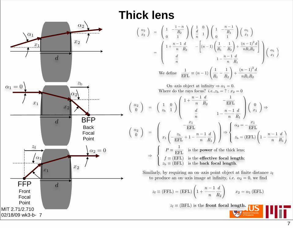
Thick lens

MIT 2.71/2.710

BFP Back Focal Point

FFP Front Focal Point

02/18/09 wk3-b- 7

7

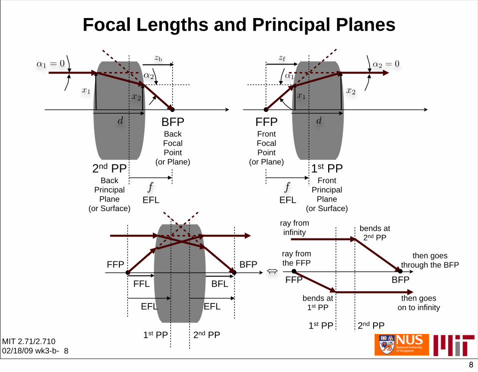
Focal Lengths and Principal Planes

BFP Back Focal Point

(or Plane)2nd PP

Back Principal

Plane (or Surface)

EFL

ray from infinity bends at

2nd PP

ray from the FFP

FFP Front Focal Point

(or Plane) 1st PP

Front Principal

Plane (or Surface)

EFL

FFP

1st PP 2nd PP

BFP

FFL BFL

EFL EFL

FFP BFP

bends at then goes 1st PP on to infinity

1st PP 2nd PP MIT 2.71/2.710 02/18/09 wk3-b- 8

then goes through the BFP

8

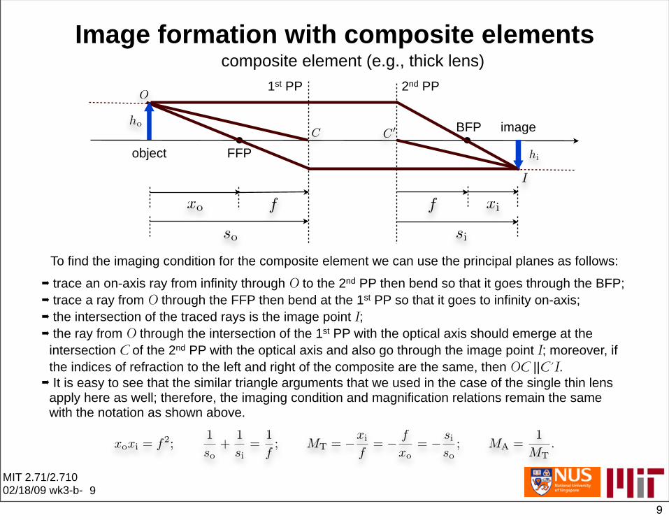
Image formation with composite elements composite element (e.g., thick lens)

object FFP

BFP image

1st PP 2nd PP

To find the imaging condition for the composite element we can use the principal planes as follows: ➡ trace an on-axis ray from infinity through O to the 2nd PP then bend so that it goes through the BFP; ➡ trace a ray from O through the FFP then bend at the 1st PP so that it goes to infinity on-axis; ➡ the intersection of the traced rays is the image point I; ➡ the ray from O through the intersection of the 1st PP with the optical axis should emerge at the

intersection C of the 2nd PP with the optical axis and also go through the image point I; moreover, if the indices of refraction to the left and right of the composite are the same, then OC ||C’I.

➡ It is easy to see that the similar triangle arguments that we used in the case of the single thin lens apply here as well; therefore, the imaging condition and magnification relations remain the same with the notation as shown above.

MIT 2.71/2.710 02/18/09 wk3-b- 9

9

Imaging systems in nature: chambered eyes

Image removed due to copyright restrictions. Please see Fig. 1 a,c,d,g in Fernald, Russell D. "Casting a Genetic Light on the Evolution of Eyes." Science 313 (2006): 1914-1918.

MIT 2.71/2.710 02/18/09 wk3-b-10

10

Imaging systems in nature: compound eyes

Image removed due to copyright restrictions. Please see Fig. 1 b, e, f, h in Fernald, Russell D. "Casting a Genetic Light on the Evolution of Eyes." Science 313 (2006): 1914-1918.

MIT 2.71/2.710 02/18/09 wk3-b-11

11

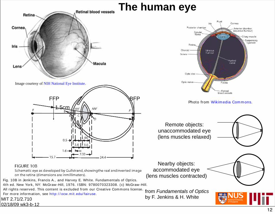
The human eye

Photo from Wikimedia Commons.

Image courtesy of NIH National Eye Institute.

Remote objects: unaccommodated eye (lens muscles relaxed)

Nearby objects: accommodated eye

(lens muscles contracted)

from Fundamentals of OpticsMIT 2.71/2.710 by F. Jenkins & H. White 02/18/09 wk3-b-12

FFP 1.5cm

BFP

12

Fig. 10B in Jenkins, Francis A., and Harvey E. White. Fundamentals of Optics.4th ed. New York, NY: McGraw-Hill, 1976. ISBN: 9780070323308. (c) McGraw-Hill. All rights reserved. This content is excluded from our Creative Commons license. For more information, see http://ocw.mit.edu/fairuse.

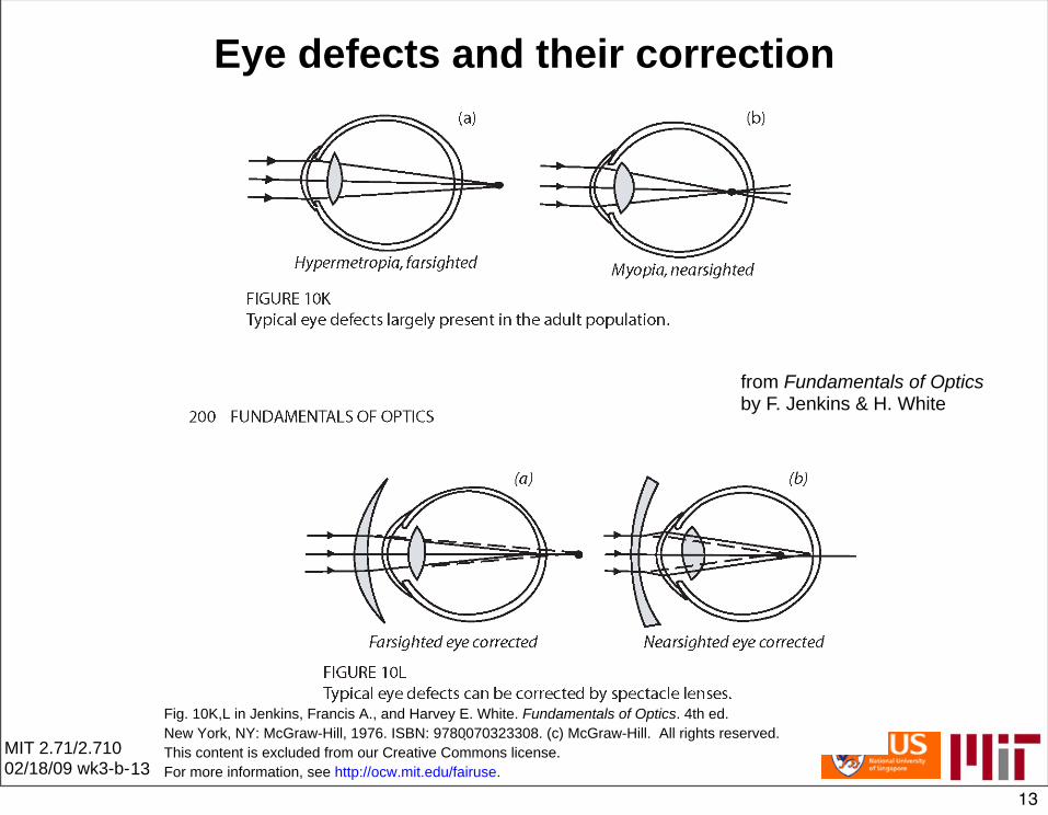
Eye defects and their correction

MIT 2.71/2.710 02/18/09 wk3-b-13

from Fundamentals of Optics by F. Jenkins & H. White

13

.Fig. 10K,L in Jenkins, Francis A., and Harvey E. White. Fundamentals of Optics. 4th ed.New York, NY: McGraw-Hill, 1976. ISBN: 9780070323308. (c) McGraw-Hill. All rights reserved.This content is excluded from our Creative Commons license.For more information, see http://ocw.mit.edu/fairuse.

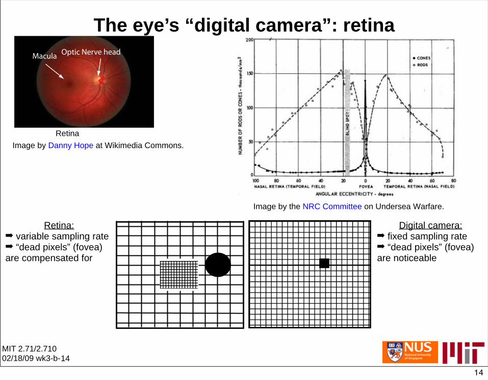
The eye’s “digital camera”: retina Macula Optic Nerve head

Image by Danny Hope at Wikimedia Commons.

Image by the NRC Committee on Undersea Warfare.

Retina: Digital camera: ➡ variable sampling rate ➡ fixed sampling rate ➡ “dead pixels” (fovea) ➡ “dead pixels” (fovea) are compensated for are noticeable

MIT 2.71/2.710 02/18/09 wk3-b-14

14

Retina

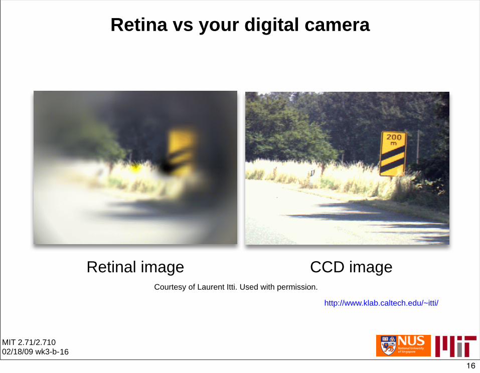
Retina vs your digital camera

Retinal image CCD image Courtesy of Laurent Itti. Used with permission.

http://www.klab.caltech.edu/~itti/

MIT 2.71/2.710 02/18/09 wk3-b-16

16

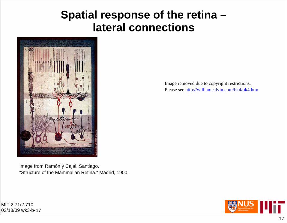
Spatial response of the retina – lateral connections

Image from Ramón y Cajal, Santiago. "Structure of the Mammalian Retina." Madrid, 1900.

MIT 2.71/2.710 02/18/09 wk3-b-17

17

Image removed due to copyright restrictions.Please see http://williamcalvin.com/bk4/bk4.htm

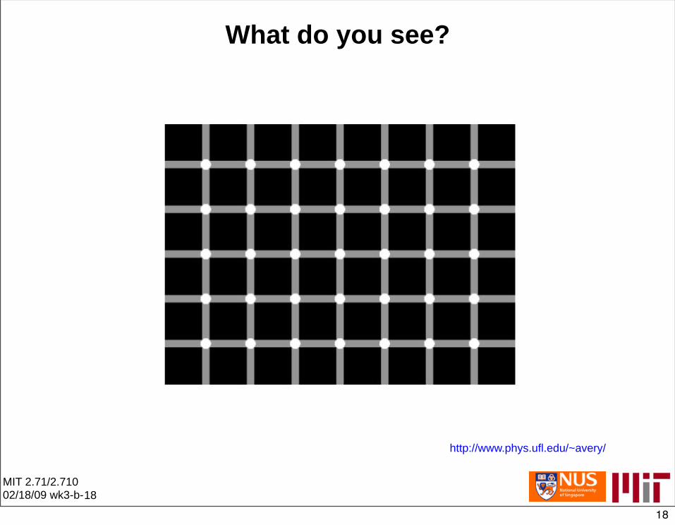
What do you see?

http://www.phys.ufl.edu/~avery/

MIT 2.71/2.710 02/18/09 wk3-b-18

18

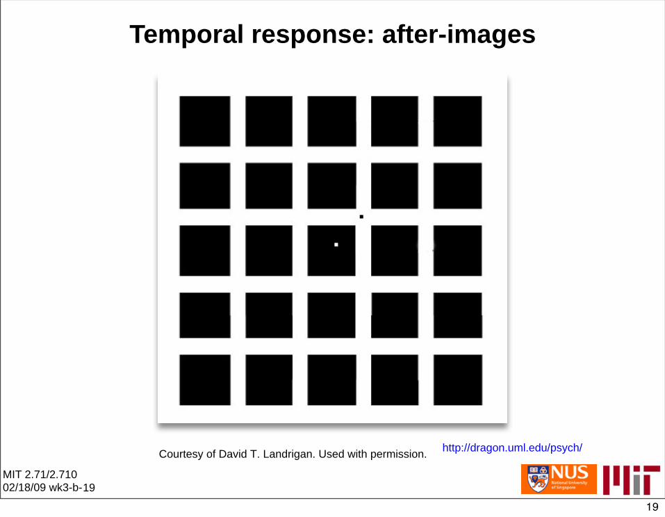
Temporal response: after-images

Courtesy of David T. Landrigan. Used with permission.

MIT 2.71/2.710 02/18/09 wk3-b-19

http://dragon.uml.edu/psych/

19

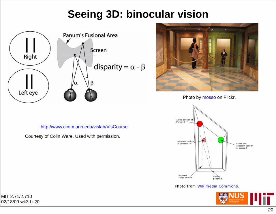
Seeing 3D: binocular vision

Photo by mosso on Flickr.

http://www.ccom.unh.edu/vislab/VisCourse

Courtesy of Colin Ware. Used with permission.

MIT 2.71/2.710 02/18/09 wk3-b-20

20

Photo from Wikimedia Commons.

MIT OpenCourseWarehttp://ocw.mit.edu

2.71 / 2.710 Optics Spring 2009

For information about citing these materials or our Terms of Use, visit: http://ocw.mit.edu/terms.