images of sagittarius a*
TRANSCRIPT
MNRAS 000, 1–9 (2017) Preprint 8 May 2018 Compiled using MNRAS LATEX style file v3.0
The impact of Faraday effects on polarized black holeimages of Sagittarius A*.
Alejandra Jimenez-Rosales? and Jason Dexter†Max-Plack-Institut fur Extraterrestrische Physik, Giessenbachstr. 1, 85748 Garching, Germany
Accepted XXX. Received YYY; in original form ZZZ
ABSTRACTWe study model images and polarization maps of Sagittarius A* at 230 GHz. Wepost-process GRMHD simulations and perform a fully relativistic radiative transfercalculation of the emitted synchrotron radiation to obtain polarized images for a rangeof mass accretion rates and electron temperatures. At low accretion rates, the polar-ization map traces the underlying toroidal magnetic field geometry. At high accretionrates, we find that Faraday rotation internal to the emission region can depolarize andscramble the map. We measure the net linear polarization fraction and find that highaccretion rate “jet-disc” models are heavily depolarized and are therefore disfavoured.We show how Event Horizon Telescope measurements of the polarized “correlationlength” over the image provide a model-independent upper limit on the strength ofthese Faraday effects, and constrain plasma properties like the electron temperatureand magnetic field strength.
Key words: accretion – black hole physics – Galaxy: centre – MHD – polarization– radiative transfer
1 INTRODUCTION
The compact radio source Sagittarius A* (Sgr A*) is theclosest supermassive black hole candidate to Earth (e.g.,Genzel et al. 2010; Falcke & Markoff 2013). With a massM ∼ 4.3 × 10⁶ solar masses and at a distance D ∼ 8.3 kpc(Boehle et al. 2016; Gillessen et al. 2017), Sgr A* is the blackhole with the largest apparent angular size on the sky (witha shadow of ∼ 50µas1), which makes it an excellent labora-tory for studying accretion physics around black holes andfor probing general relativistic effects. Sgr A* emits most ofits luminosity from synchrotron radiation in what is calledthe “submillimetre bump.” At these wavelengths (. 1 mm),the radiation is expected to be optically thin and originatefrom close to the black hole (Falcke & Markoff 2000; Boweret al. 2015).
Models of radiatively inefficient accretion flows (RIAFsNarayan & Yi 1995; Quataert & Narayan 1999; Yuan et al.2003) and magnetised jets (Falcke & Markoff 2000; Yuanet al. 2002) have been developed to explain the radio spec-trum of Sgr A*. Such models can now be realised using gen-eral relativistic magnetohydrodynamic (GRMHD) simula-
? E-mail: [email protected]† E-mail: [email protected] The angular size of Sgr A* is given by Rs/D ∼ 10 µas, whereRs ∼ 1.36 × 1012 cm is the Schwarzschild radius.
tions, which capture the time-dependent accretion processas a result of the magnetorotational instability (MRI, Bal-bus & Hawley 1991) including all relativistic effects. This isparticularly important for interpreting mm-VLBI data fromthe Event Horizon Telescope (EHT), which now resolves theemission at 230 GHz on event horizon scales. The compactsize found for Sgr A* is ' 4 Schwarzschild radii (Doelemanet al. 2008; Fish et al. 2011).
Total intensity images of submm synchrotron emissionfrom such models predict somewhat different morphologies(size, degree of asymmetry) due to differences in the initialconditions, such as magnetic field configuration, electron-proton coupling, electron temperature distribution functionand evolution, to name a few. Although any particular modelis well constrained (e.g., Dexter et al. 2010; Broderick et al.2011), the images are often dominated by the relativistic ef-fects of light bending and Doppler beaming due to an emis-sion radius close to the event horizon, resulting in a char-acteristic crescent shape (e.g., Bromley et al. 2001; Brod-erick & Loeb 2006; Moscibrodzka et al. 2009; Dexter et al.2010; Kamruddin & Dexter 2013; Moscibrodzka et al. 2014;Chan et al. 2015; Ressler et al. 2017). As a result, model-dependence in parameter estimation from total intensity im-ages is a major current issue.
The discovery of 5−10% linear polarization from Sgr A*at 230 GHz (Aitken et al. 2000) showed that the accretionrate is much less than that inferred from X-ray observa-
© 2017 The Authors
arX
iv:1
805.
0265
2v1
[as
tro-
ph.H
E]
7 M
ay 2
018

2 A. Jimenez-Rosales et al.
tions (Baganoff et al. 2001) of hot gas at the Bondi radius(Agol 2000; Quataert & Gruzinov 2000). At the Bondi accre-tion rate, the internal Faraday rotation within the emittingplasma should depolarize the synchrotron radiation at 230GHz. Later detections of external Faraday rotation allow anestimate of the accretion rate ∼ 10−9 − 10−7M� yr−1 (Boweret al. 2003; Marrone et al. 2006), a factor ' 100 smaller thanthe Bondi value.
EHT observations provide the opportunity to measurethe spatially resolved polarization, and show that this frac-tion can rise to up to 20−40% on event horizon scales (John-son et al. 2015). They interpret this as evidence for a bal-ance of order and disorder in the underlying polarizationmap, which can be well matched by maps from GRMHDsimulations (Gold et al. 2017).
Here we use polarized radiative transfer calculations ofa single snapshot from an axisymmetric GRMHD simulation(§2) to understand how the resulting polarization propertiesdepend on the physical parameters of the emitting plasma.We show that internal Faraday effects become strong in asignificant range of model parameter space, scrambling anddepolarizing the resulting polarization maps (§3). Measur-ing the correlation length of the polarization direction fromspatially resolved data provides the cleanest way to set lim-its on the underlying properties of the plasma. We show howthis can be measured from future EHT data as a novel con-straint on the mass accretion rate and electron temperatureof the Sgr A* accretion flow.
2 ACCRETION FLOW AND EMISSIONMODELS
We consider a snapshot of a 2D axisymmetric numerical so-lution (Dexter et al. 2010) from the public version of theGRMHD code HARM (Gammie et al. 2003; Noble et al.2006), where the initial conditions consist of a rotating blackhole with dimensionless spin a = 0.9375 surrounded by atorus in hydrostatic equilibrium (Fishbone & Moncrief 1976)threaded with a weak poloidal magnetic field. The systemevolves according to the ideal MHD equations in the Kerrspacetime.2 Turbulence due to the MRI produces stresseswithin the torus and leads to an outward transport of angu-lar momentum, causing accretion of material onto the blackhole.
Synchrotron radiation is produced by the hot, magne-tised plasma and travels through the emitting medium. Inthe absence of any other effects, the resulting polarizationconfiguration seen by a distant observer traces the mag-netic field structure of the gas.3 However, as light travelsthe polarization angle is rotated both by parallel transportin the curved spacetime near the black hole and by Faradayrotation in the magnetised accretion flow, the latter being
2 Our snapshot is taken at time t = 2000 GM/c3, where G is the
gravitational constant, M is the mass of the black hole and c is
the light speed.3 So that the emitted polarization vector is perpendicular to
the local magnetic field direction, we use EVPA = 1/2 tan−1(U/Q),where EVPA is the electric vector position angle and Q and Uare Stokes parameters.
characterised by the Faraday rotation depth, τρV =∫ρV dl,
where
ρV = (e3/πm2e c2) cos θBneB f (Te , ®B)/ν2; (1)
ρV is the Faraday rotation coefficient, e,me, ne are the elec-tron charge, mass and number density respectively, θB isthe angle between the line of sight and the magnetic field ®Bwith | ®B| = B, c and ν are the light speed and frequency, andf (Te , ®B) is a function of ®B and the electron temperature Te,but approximately f ≈ T−2
e (Jones & Hardee 1979; Quataert& Gruzinov 2000). All quantities are measured in the comov-ing orthonormal fluid frame (Shcherbakov & Huang 2011;Dexter 2016).
MHD simulations without radiation self-consistentlyevolve Pgas/n ∼ Tp and B2/n, where Pgas is the gas pres-sure, n and Tp are the proton density and temperature re-spectively. Choosing the black hole mass sets the lengthand timescales, while the mass accretion rate ÛM is a freeparameter which sets the density scale. The electron tem-perature Te is not self-consistently computed, and one mustmake a choice for it. Different approaches have been takento parametrise Te, from a constant Tp/Te within the accre-tion flow (Moscibrodzka et al. 2009) to directly evolving itwith the fluid (Ressler et al. 2015, 2017; Chael et al. 2018)assuming some electron heating prescription (Howes 2010;Rowan et al. 2017; Werner et al. 2018). We assume thatTe(η , α) = η Tp/α, with η ∈ (0 , 1] a constant ratio betweenthe electron and proton temperatures and α = α(µ , β) afunction that depends on the magnetisation of the plasmasimilar to the one used in Moscibrodzka et al. (2016): 4
α = µβ2
1 + β2 +1
1 + β2 , (2)
where the plasma parameter β = Pgas/Pmag states the ratiobetween the gas and magnetic pressures and µ is a free pa-rameter that describes the electron to proton coupling in theweakly magnetised zones (disc body) of the simulation.
The numerical solution we use has a Blandford-Znajekjet (McKinney 2006). Different choices of µ, the electron-proton coupling factor in Eq. 2, can cause the wall betweenthe accretion flow and the jet to shine. When µ in equation2 is small, the disc has a very high temperature and lightsup at 230 GHz due to the fact that, compared to the jet,it has both the highest density and magnetic field strength.However, the larger the µ the colder the disc is and thefainter it gets. If one wishes to maintain a fixed flux, theaccretion rate onto the black hole ÛM must increase. As aconsequence, the jet wall can light up first even given itslower density and field strength.
For a given choice of η and µ = (1 , 2 , 5 , 10 , 40 , 100), ÛM isthen chosen in such a way that the total flux Fν at 230 GHz iseither 3 Jy or 0.3 Jy. We chose the first value to model Sgr A*and the second, 0.3 Jy, arbitrarily to decrease αI/ρV , whereαI is the total absorption coefficient. This second option forFν gives us the opportunity to study models in the opticallythin regime to separate the effects of absorption and Faradayrotation.
Given that ne ∝ ÛM, B ∝ ÛM1/2, Fν ∝ nξe BκTeσ (where
4 We have taken µ = Rhigh and Rlow = 1 in the (Moscibrodzka
et al. 2016) expression.
MNRAS 000, 1–9 (2017)

Faraday effects and Sgr A* polarization. 3
typically ξ ∈ [0, 1], κ ∈ [0, 2], σ ∈ [1, 4]), and assuming aconstant Fν , we can express the Faraday rotation depth, τρV ,as a function of ÛM:
τρV ∼ neBTe−2 ∝ ÛMδ ; (3)
where δ ≡ 3/2+ (2ξ+ κ)/σ ' 3/2−7/2. It can be seen from eq.3 that τρV has a strong dependence on ÛM and small changesof this quantity reflect as big differences in τρV . Due to this,models with similar physical parameters can vary widely inthe strength of the internal Faraday effects and, for τρV & 1,in the resulting polarization structure.
To account for emission, absorption, parallel transportand Faraday effects locally within the accretion flow, we em-ploy the publicly available numerical code grtrans (Dex-ter & Agol 2009; Dexter 2016)5 to do a self-consistent fullyrelativistic ray tracing radiative transfer calculation at 230GHz. The output of the calculation is a polarized image ofour GRMHD snapshot as seen by a distant observer at a 50degree inclination from the black hole (and accretion flow)rotation axis.
3 RESULTS
Fig. 1 shows the resulting intensity-weighted, image-averaged electron temperature 〈Te〉, polar angle 〈cos θ〉, andFaraday rotation depth 〈τρV 〉 for each input model withvarying ( ÛM,Te). The steady decrease of 〈Te〉 with ÛM in theupper left panel of Fig 1 points to “disc-like” systems. Thetransition to “jet-like” systems happens when the circlesshow a constant behaviour with ÛM and is highly dependenton µ. As discussed before, at large µ the jet has a high enoughtemperature that it can outshine the cold disc.
This is shown as well in the right panel of Fig. 1, wherethe cosine of the inclination angle where most of the emissioncomes from, 〈cos θ〉, as a function of ÛM is plotted. It can beseen that at high ÛM, models that have the same accretionrate but different µ values have different emission regions.As the electron-proton coupling µ increases, the emissionregion moves towards the poles indicating a transition to amore “jet-like” system.
In the bottom panel of Fig. 1 we plot the intensity-weighted image-averaged Faraday rotation depth 〈τρV 〉 vsÛM and the scaling relation in eq. 3, with δ = 2.6 This panel
shows very nicely the wide spread in 〈τρV 〉 values as a func-tion of ÛM, supporting the idea that systems with similarphysical parameters can have widely varying strengths ofFaraday rotation. This makes 〈τρV 〉 a sensitive tracer of thephysical conditions of the plasma.
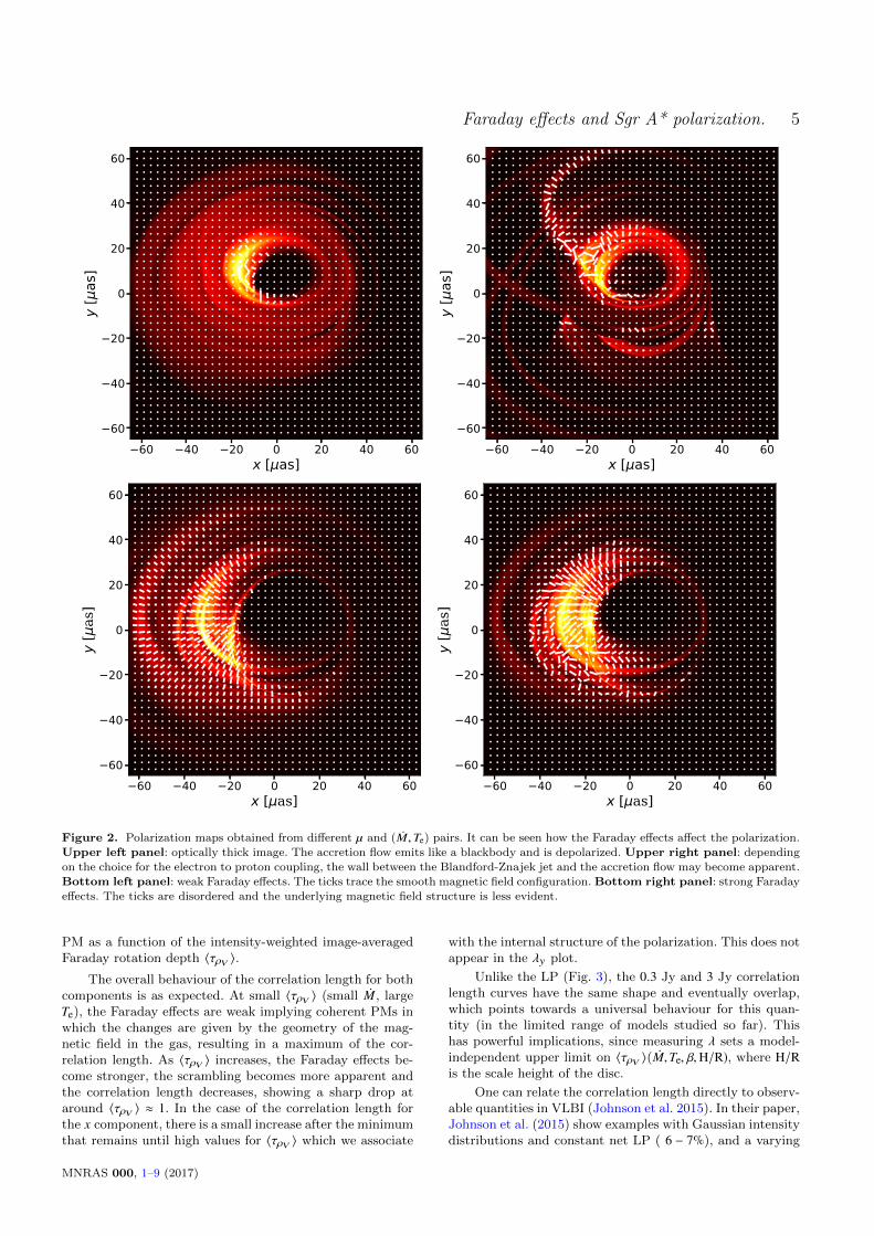
Fig. 2 shows four sample polarized images. Plotted inthe background is the total intensity image centred on theblack hole (colour shows total flux on a linear scale wherethe lighter the shade the greater the emission).
These images show the accreting material in character-istic asymmetric crescent shapes: due to Doppler beaming inthe rotation torus, the left side where the gas approaches theobserver is much brighter than the right side. Furthermore,
5 http://www.github.com/jadexter/grtrans6 We included the effects of Faraday conversion in the radiativetransfer calculation as well, but it is significantly weaker than
Faraday rotation, and so we focus our study to the latter.
strong relativistic light bending lets us see behind the blackhole, whose emission appears to be coming from above andbelow it in the images. In the foreground, white ticks showlinear polarization fraction (LP) direction with their length
proportional to the LP magnitude (given by√
Q2 +U2). Thisis what we refer to as a polarization map (PM).
The images shown in Fig. 2 have a variety of model pa-rameters. In the upper left panel an optically thick image isshown. In this case, the system resembles a black body, dom-inated by optical absorption and is completely depolarizedfrom self-absorption. We can see a case of the Blandford-Znajek jet wall lighting up in the upper right panel of Fig.2 for a case where µ = 100.
The bottom panels of Fig 2 are optically thin. In thecase of weak Faraday effects (hot, tenuous emitting medium- high Te and low ÛM, 〈τρV 〉 < 1; bottom left panel), thepolarization traces the toroidal magnetic field (horizontalwhere the light comes from the approaching gas and ver-tical where it comes from gas behind the black hole) anddisplays an ordered behaviour (due to the axisymmetry ofthe system). The combination of this with the crescent shapebackground image leads to such a characteristic polarizationmap (Bromley et al. 2001). When considering the polariza-tion over the whole image, the contributions from each ofthe vector components may cancel, resulting in a lower LPover the image (beam depolarization). Strong Faraday effects(colder, denser medium - low Te, high ÛM; bottom right panelof Fig. 2) can scramble and depolarize the image on smallscales.
3.1 Linear Polarization Fraction and RotationMeasure in the models.
Fig. 3 shows the net intensity-weighted LP integrated overthe image versus the intensity-weighted image-averagedFaraday rotation depth, 〈τρV 〉. The images generally depo-larize with increasing 〈τρV 〉, as expected. However, the in-dividual behaviour between both sets of models (diamondsand circles) is different, and no smooth or uniform LP trendas a function of 〈τρV 〉 can be extracted.
Given a measurement of LP, one could use Fig. 3 to setan upper limit on 〈τρV 〉 and obtain the models that satisfythe restriction set by the LP. As an example, a variety ofour “disc-like” models where 〈τρV 〉 varies over many orders
of magnitude (∼ 5×10⁻²−1×10²) satisfy the measured 5−10%LP for Sgr A* at 230 GHz (Aitken et al. 2000). The emis-sion is locally strongly polarized (& 40%) but is naturallybeam depolarized due to the combination of the crescentimage and toroidal magnetic field configuration. The “jet-like” models ( 〈τρV 〉 & 102) on the other hand are heavilydepolarized, and cannot match the observed LP of Sgr A*.
We looked at the dependence of the rotation measure(RM) of the images with 〈τρV 〉 as well and found, as ex-pected, that the RM increases with 〈τρV 〉. However, we couldnot get a clean measurement like in Bower et al. (2003) andMarrone et al. (2006) because our simulation domain is notas large as that in their work. We can look at this in thefuture, but it would require very long duration simulations(e.g., Narayan et al. 2012) to reach inflow equilibrium at thelarge radii of the external Faraday screen.
MNRAS 000, 1–9 (2017)

4 A. Jimenez-Rosales et al.
10 10 10 9 10 8
Accretion rate M [M /yr]
1010
1011
Ele
ctro
n te
mpe
ratu
re T
e [
K]
F = 0.3 =1F = 0.3 =2F = 0.3 =5F = 3.0 =1F = 3.0 =2F = 3.0 =5F = 3.0 =10F = 3.0 =40F = 3.0 =100
10 10 10 9 10 8
Accretion rate M [M /yr]
0.1
0.2
0.3
0.4
0.5
Pola
r an
gle
cos
F = 0.3 =1F = 0.3 =2F = 0.3 =5F = 3.0 =1F = 3.0 =2F = 3.0 =5F = 3.0 =10F = 3.0 =40F = 3.0 =100
10 10 10 9 10 8
Accretion rate M [M /yr]
10 1
100
101
102
103
104
105
106
Fara
day
rota
tion
dept
h V
V
M2
F = 0.3 =1F = 0.3 =2F = 0.3 =5F = 3.0 =1F = 3.0 =2F = 3.0 =5F = 3.0 =10F = 3.0 =40F = 3.0 =100
Figure 1. Intensity-weighted, image-integrated model quantities. Each dot is a chosen ( ÛM, Te) pair with Fν indicated by a colour scale:
diamonds for Fν = 0.3 Jy and circles for Fν = 3 Jy. The colour gradient shows the choice for µ, where the lighter (darker) the shade, thelower (higher) the µ value is. Upper left: Intensity-weighted, image-averaged electron temperature 〈Te 〉 vs ÛM . The models that show a
steady decrease of 〈Te 〉 with ÛM are more “disc-like” systems. The transition to “jet-like” systems happens where the decrement stops and
becomes constant with ÛM . Upper right: Intensity-weighted image-averaged emission angle 〈cos θ 〉 as a function of ÛM . At high ÛM , as µincreases the emission region moves towards the poles, indicating the transition to a more “jet-like” system. Bottom: Intensity-weighted
image-averaged Faraday rotation depth 〈τρV 〉 vs ÛM . It can be seen how 〈τρV 〉 extends over a wide range of values with ÛM . A scaling
relation between both quantities is shown with a dotted line where δ = 2.
3.2 The Correlation Length.
The upper panels of Fig 2 can be easily distinguished fromtheir total intensity images alone and might be disfavouredalready from the measured size of the source and spectralobservations. In the optically thin regimes however (bottompanels), the total intensity images are hard to tell apart andare generally consistent with the observational constraints(Moscibrodzka et al. 2009; Dexter et al. 2010). The polar-ization maps however, vary substantially. This spatial con-figuration of the polarization offers an alternative to learningabout the physical parameters of the models.
To characterise the degree of order of each map pro-duced by a particular ( ÛM, Te) pair, we use a quantity whichwe call the “correlation length”, λ. Large values of λ point toan ordered configuration, limited by the coherence of themagnetic field structure, whereas small values indicate amore disordered configuration.
To calculate this quantity we autocorrelate each map.Because the PM is a vector field, we look at each componentseparately and weight their value at each pixel by Stokes Iat the same pixel7 (left panel of Fig. 4). The result is a 2Dfunction that gives information on how the polarization com-ponent varies spatially. We then take 50 “1D slices” of thisfunction in different angular directions to account for thespatial changes in 2D and take the average of their widthsat 0.5 (FWHM, middle and right panels of Fig. 4). Twicethis value is the polarized correlation length in µas.
Figure 5 shows the correlation length (λx and λy , x andy subindices for each vector component) of each simulation’s
7 The reference system is orthonormal with one of the axesaligned with the spin axis of the black hole and the other in adirection perpendicular to the observer (Bardeen et al. 1972).
MNRAS 000, 1–9 (2017)
Faraday effects and Sgr A* polarization. 5
60 40 20 0 20 40 60x [ as]
60
40
20
0
20
40
60
y [
as]
60 40 20 0 20 40 60x [ as]
60
40
20
0
20
40
60
y [
as]
60 40 20 0 20 40 60x [ as]
60
40
20
0
20
40
60
y [
as]
Figure 2. Polarization maps obtained from different µ and ( ÛM, Te) pairs. It can be seen how the Faraday effects affect the polarization.Upper left panel: optically thick image. The accretion flow emits like a blackbody and is depolarized. Upper right panel: depending
on the choice for the electron to proton coupling, the wall between the Blandford-Znajek jet and the accretion flow may become apparent.
Bottom left panel: weak Faraday effects. The ticks trace the smooth magnetic field configuration. Bottom right panel: strong Faradayeffects. The ticks are disordered and the underlying magnetic field structure is less evident.
PM as a function of the intensity-weighted image-averagedFaraday rotation depth 〈τρV 〉.
The overall behaviour of the correlation length for bothcomponents is as expected. At small 〈τρV 〉 (small ÛM, largeTe), the Faraday effects are weak implying coherent PMs inwhich the changes are given by the geometry of the mag-netic field in the gas, resulting in a maximum of the cor-relation length. As 〈τρV 〉 increases, the Faraday effects be-come stronger, the scrambling becomes more apparent andthe correlation length decreases, showing a sharp drop ataround 〈τρV 〉 ≈ 1. In the case of the correlation length forthe x component, there is a small increase after the minimumthat remains until high values for 〈τρV 〉 which we associate
with the internal structure of the polarization. This does notappear in the λy plot.
Unlike the LP (Fig. 3), the 0.3 Jy and 3 Jy correlationlength curves have the same shape and eventually overlap,which points towards a universal behaviour for this quan-tity (in the limited range of models studied so far). Thishas powerful implications, since measuring λ sets a model-independent upper limit on 〈τρV 〉( ÛM,Te, β,H/R), where H/Ris the scale height of the disc.
One can relate the correlation length directly to observ-able quantities in VLBI (Johnson et al. 2015). In their paper,Johnson et al. (2015) show examples with Gaussian intensitydistributions and constant net LP ( 6 − 7%), and a varying
MNRAS 000, 1–9 (2017)

6 A. Jimenez-Rosales et al.
10 1 100 101 102 103 104 105 106
Faraday rotation depth V
0.0
2.5
5.0
7.5
10.0
12.5
15.0
17.5
20.0
Line
ar P
olar
izat
ion
[ % ]
F = 0.3 =1F = 0.3 =2F = 0.3 =5F = 3.0 =1F = 3.0 =2F = 3.0 =5F = 3.0 =10F = 3.0 =40F = 3.0 =100
Figure 3. Net linear polarization fraction plotted against the intensity-weighted image-averaged Faraday rotation depth 〈τρV 〉. The
same colour and marker criteria has been used as that in figure Fig. 1. As the Faraday effects become stronger, the LP decreases, as
expected. However the behaviour is neither smooth nor universal ( 〈τρV 〉 . 102). “Jet-like” models have high Faraday optical depths (〈τρV 〉 & 102) from the cold, dense disc and are heavily depolarized, failing to reproduce the Sgr A* LP of ' 5 − 10%.
60 40 20 0 20 40 60x [ as]
60
40
20
0
20
40
60
y [
as]
x component
0 10 20 30 40 50 60x [ as]
0
10
20
30
40
50
60
y [
as]
Autocorrelation function
0 10 20 30 40 50 60x [ as]
0.0
0.2
0.4
0.6
0.8
1.0Au
toco
rrel
atio
n fu
nctio
n va
lues
FWHM = 15.633 [ as]
Correlation length: x = 31.265 [ as]
1D slices
Figure 4. Illustration of the calculation of the polarized correlation length. Left: take one of the vector components of the polarization(x component shown here) and auto-correlate the map. Middle: Plotted in the background in shades of purple is the 2D autocorrelation
function. We take 1D slices of this function in different angular directions (coloured solid lines in the foreground) to account for the 2D
behaviour. Right: 1D slices from the autocorrelation function. Twice the average of their values at 0.5 (FWHM) is how we define as thepolarized correlation length, λx , in µas.
polarization structure with a prescribed coherence length.They find a correlation length of 0.29 times the GaussianFWHM of the model. Measuring an approximate GaussianFWHM for our images and multiplying it by 0.29 gives usan estimated correlation length of 11.6µas. We then useFig. 5 to set an upper limit on the 〈τρV 〉 . 1, in agreementwith the qualitative argument of Agol (2000) and Quataert& Gruzinov (2000). However, our models are not Gaussiansand it is not clear that the λ value inferred by Johnson et al.(2015) applies here.
We can extend the analysis further into visibility space.Fig. 6 shows the Stokes parameters I, Q and U (top) andtheir respective visibilities I, Q and U (bottom) of one of
our simulations. On large scales, it can be seen that Q and Uresemble I, showing the same crescent structure. However,on smaller scales some deviation becomes evident becausethe polarization, ®p, is changing. Therefore, on the largestscales one gets information on I and on the smallest scalesone sees the polarization properties.
If we study this in the visibility space uv and take theFourier Transform (FT) of the Stokes parameters (bottomimages of Fig. 6), the roles are inverted. Large scale featuresbecome small and vice versa. In this respect, the shape of thetotal intensity image becomes a small “beam” in uv, whereasthe large scale structure observed in the Q and U images
MNRAS 000, 1–9 (2017)

Faraday effects and Sgr A* polarization. 7
10 1 100 101 102 103 104 105 106
Faraday rotation depth V
0
5
10
15
20
25
30
35
Cor
rela
tion
leng
th
x [
as]
F = 0.3 =1F = 0.3 =2F = 0.3 =5F = 3.0 =1F = 3.0 =2F = 3.0 =5F = 3.0 =10F = 3.0 =40F = 3.0 =100
10 1 100 101 102 103 104 105 106
Faraday rotation depth V
0
5
10
15
20
25
30
35
Cor
rela
tion
leng
th
y [
as]
F = 0.3 =1F = 0.3 =2F = 0.3 =5F = 3.0 =1F = 3.0 =2F = 3.0 =5F = 3.0 =10F = 3.0 =40F = 3.0 =100
Figure 5. Correlation length measured for x and y vector components (left and right panels respectively) of PMs with different µ and
( ÛM ,Te) values plotted against the intensity-weighted image-averaged Faraday rotation depth 〈τρV 〉. The same colour and marker criteria
is used as that in Fig. 1 and Fig. 3. Coherent maps are obtained when 〈τρV 〉 . 1 and scrambling appears as the Faraday effects becomestronger. A measurement of the correlation length places a model-independent upper limit on 〈τρV 〉, and in turn the lower limits on the
plasma electron temperature and relative magnetic field strength.
corresponds to the smallest angular scales in Q and U andreflects the properties of the polarization map.
One can think of the images as the convolution of I with®p, with the result interpreted as I being smeared out by ®pwith some characteristic scale that reflects the inner struc-ture of the latter. In the case of a completely disordered po-larization map, taking the FT of the image would give whatwould basically be a noise map in the visibility space, withno characteristic scale at which the polarization’s behaviourstands out. On the other hand, the FT of the convolutionbetween I and a completely ordered ®p would give an imagewith a nice beam centred at uv = 0 and no noise whatsoever.
We are interested in finding the characteristic scale atwhich the random fluctuations or noise in the polarizationis suppressed. We call this the polarized correlation lengthof the visibility, λx , where x is one of the Stokes parameters.
We measure this as the uv distance at which the visibil-ity’s amplitude drops permanently below a certain value. Asan example, we have chosen this quantity to be 10% of Qmaxand Umax, where Qmax and Umax are the maximum visibilityamplitudes. We define the visibility correlation length as theinverse of the averaged distances which satisfy this criteria.The calculated λ
Qand λ
Ufor our models are shown in Fig.
7.As shown in Fig. 7, the correlation length measured in
the visibility space can also constrain 〈τρV 〉 and is measureddirectly from VLBI observables. With upcoming data fromthe EHT, this quantity may be promising for inferring thecharacteristics of the plasma in the system.
4 DISCUSSION
Sgr A* is a great laboratory for testing accretion physicsand general relativity. Polarization is a powerful tool fordetermining the plasma properties and the magnetic fieldstructure.
From a GRMHD simulation of a torus of magnetisedplasma in initial hydrostatic equilibrium with a poloidalmagnetic field, we have done self-consistent fully relativisticray tracing radiative transfer calculations of the radiation at230 GHz. We have analysed the different polarized imagesand characterised the degree of coherence in the polariza-tion map as a function of the Faraday rotation depth. Thiscoherence scale we call the correlation length. Large valuesof this quantity are expected when the Faraday effects areweak and the maps are ordered. Small values of the corre-lation length in our models point to large Faraday rotationdepth values and disordered maps.
We have proposed a method to relate the polarized cor-relation length calculated from the images to direct observ-ables of VLBI by taking the Fourier Transform of the imagesand analysing the large scale structure of the visibilities inthe Fourier domain. This shows a similar behaviour to thatshowed in the image space, with the advantage that it usesVLBI observables.
In the past, unresolved polarization of Sgr A* has beenvery helpful in constraining models. With the new EHT mea-surements this can be done with the polarization map itselffor the first time through the correlation length. So far, thebehaviour of this new quantity appears to be model inde-pendent, which makes it a promising approach that can beused to set restrictions on the plasma parameters around theblack hole and distinguish models robustly in a way that isoften difficult with total intensity images alone.
Constraining 〈τρV 〉 ∼ neBT−2e places limits on the phys-
ical properties of the accreting gas, most directly Te. In ad-dition, B2 ∼ β−1nTp. From hydrostatic equilibrium, Tp ∼Tvir(H/R)2, where Tvir ∼ mpc2/r is the virial temperature atdimensionless radius r = R/Rs and H/R is the scale heightof the accretion flow. The relative field strength then scalesas B2/n ∼ β−1(H/R)2. At fixed flux density, a limit on 〈τρV 〉
MNRAS 000, 1–9 (2017)

8 A. Jimenez-Rosales et al.
50 25 0 25 50x [ as]
60
40
20
0
20
40
60
y [
as]
Stokes I
50 25 0 25 50x [ as]
60
40
20
0
20
40
60
y [
as]
Stokes Q
50 25 0 25 50x [ as]
60
40
20
0
20
40
60
y [
as]
Stokes U
5 0 5u [G ]
8
6
4
2
0
2
4
6
8
v [G
]
Visibility I
5 0 5u [G ]
8
6
4
2
0
2
4
6
8
v [G
]
Visibility Q
5 0 5u [G ]
8
6
4
2
0
2
4
6
8
v [G
]
Visibility U
Figure 6. I , Q and U Stokes parameters for one of our simulations in image (top panels) and visibility space (bottom panels). On the
top images, it can be seen that Q and U resemble I on large scales, with different substructure due to the changing polarization. On
the visibility space however (bottom panels), small scale features in Q and U give information on I whereas the large scale structure
corresponds to the polarization.
constrains a combination of the magnetic field strength anddisc scale height as well as the electron temperature.
We have only considered one inclination. We expect thatthe trend of decreasing LP and correlation length with in-creasing Faraday rotation optical depth holds at all viewinggeometries, but their maximum values at low Faraday rota-tion depth will be model-dependent.
We have also neglected the effects of interstellar scatter-ing. The diffusive part of the scattering should not affect thecorrelation length results, since we use ratios of the Stokesparameters which are all modified in the same way. The re-fractive part of the scattering (e.g., Gwinn et al. 2014) couldin particular complicate our proposed method for measuringthe correlation length in the Fourier domain, since it willintroduce signal beyond that corresponding to small scalestructure in the polarization map.
We have demonstrated the technique with a single snap-shot from an axisymmetric GRMHD simulation. This is hassome limitations given that the MRI is unsustainable in2D and the simulation can only be studied for short times.Therefore, the degree of order seen for 〈τρV 〉 < 1 (bottom leftpanel of Fig. 2) is somewhat overestimated compared to 3D
simulations. Extensions to 3D and studying time variabilityare goals for future work. The time variable polarized cor-relation length could for example be used to measure theproperties of MRI turbulence in EHT data.
We have focused here on the case of mm-VLBI of SgrA*, but the same technique should apply to M87 (Mosci-brodzka et al. 2017) or any other synchrotron source with aresolved polarization map. In particular, in polarized VLBIimages of radio jets past work has focused on measuring theFaraday rotation across the image (e.g., Zavala & Taylor2003; O’Sullivan et al. 2018). Here we have shown that thecorrelation length may be a more robust indicator of theFaraday optical depth, if there is a significant contributionfrom within the emission region.
ACKNOWLEDGEMENTS
The authors thank M. Johnson, M. Moscibrodzka, C. Gam-mie, A. Broderick, R. Gold, J. Kim, and D. P. Marronefor useful discussions related to Sgr A* polarization andradiative transfer. This work was supported by a CONA-
MNRAS 000, 1–9 (2017)

Faraday effects and Sgr A* polarization. 9
10 2 100 102 104 106
Faraday rotation depth V
10
15
20
25
30
Visi
bilit
y co
rrel
atio
n le
ngth
Q [
as]
F = 0.3 =1F = 0.3 =2F = 0.3 =5F = 3.0 =1F = 3.0 =2F = 3.0 =5F = 3.0 =10F = 3.0 =40F = 3.0 =100
10 2 100 102 104 106
Faraday rotation depth V
10
15
20
25
30
Visi
bilit
y co
rrel
atio
n le
ngth
U [
as]
F = 0.3 =1F = 0.3 =2F = 0.3 =5F = 3.0 =1F = 3.0 =2F = 3.0 =5F = 3.0 =10F = 3.0 =40F = 3.0 =100
Figure 7. Polarized correlation length in the Fourier domain using Q (left panel) and U (right panel) for our models. The criteria usedwas to take the inverse of the averaged uv distances at which the amplitude of the visibility drops below 10% of each respective visibility
maximum, Qmax and Umax for each model. As in the image domain, the correlation length drops sharply for 〈τρV 〉 & 1.
CyT/DAAD grant (57265507) and by a Sofja Kovalevskajaaward from the Alexander von Humboldt foundation.
REFERENCES
Agol E., 2000, ApJ, 538, L121
Aitken D. K., Greaves J., Chrysostomou A., Jenness T., HollandW., Hough J. H., Pierce-Price D., Richer J., 2000, ApJ, 534,
L173
Baganoff F. K., et al., 2001, Nature, 413, 45
Balbus S. A., Hawley J. F., 1991, ApJ, 376, 214
Bardeen J. M., Press W. H., Teukolsky S. A., 1972, ApJ, 178, 347
Boehle A., et al., 2016, ApJ, 830, 17
Bower G. C., Wright M. C. H., Falcke H., Backer D. C., 2003,
ApJ, 588, 331
Bower G. C., et al., 2015, ApJ, 802, 69
Broderick A. E., Loeb A., 2006, MNRAS, 367, 905
Broderick A. E., Fish V. L., Doeleman S. S., Loeb A., 2011, ApJ,735, 110
Bromley B. C., Melia F., Liu S., 2001, ApJ, 555, L83
Chael A., Rowan M. E., Narayan R., Johnson M. D., Sironi L.,2018, preprint, (arXiv:1804.06416)
Chan C.-K., Psaltis D., Ozel F., Narayan R., Sadowski A., 2015,
ApJ, 799, 1
Dexter J., 2016, MNRAS, 462, 115
Dexter J., Agol E., 2009, ApJ, 696, 1616
Dexter J., Agol E., Fragile P. C., McKinney J. C., 2010, ApJ, 717,1092
Doeleman S. S., et al., 2008, Nature, 455, 78
Falcke H., Markoff S., 2000, A&A, 362, 113
Falcke H., Markoff S. B., 2013, Classical and Quantum Gravity,30, 244003
Fish V. L., et al., 2011, ApJ, 727, L36
Fishbone L. G., Moncrief V., 1976, ApJ, 207, 962
Gammie C. F., McKinney J. C., Toth G., 2003, ApJ, 589, 444
Genzel R., Eisenhauer F., Gillessen S., 2010, Reviews of Modern
Physics, 82, 3121
Gillessen S., et al., 2017, ApJ, 837, 30
Gold R., McKinney J. C., Johnson M. D., Doeleman S. S., 2017,
ApJ, 837, 180Gwinn C. R., Kovalev Y. Y., Johnson M. D., Soglasnov V. A.,
2014, ApJ, 794, L14
Howes G. G., 2010, MNRAS, 409, L104Johnson M. D., et al., 2015, Science, 350, 1242
Jones T. W., Hardee P. E., 1979, ApJ, 228, 268
Kamruddin A. B., Dexter J., 2013, MNRAS, 434, 765Marrone D. P., Moran J. M., Zhao J.-H., Rao R., 2006, ApJ, 640,
308
McKinney J. C., 2006, MNRAS, 368, 1561Moscibrodzka M., Gammie C. F., Dolence J. C., Shiokawa H.,
Leung P. K., 2009, ApJ, 706, 497
Moscibrodzka M., Falcke H., Shiokawa H., Gammie C. F., 2014,A&A, 570, A7
Moscibrodzka M., Falcke H., Shiokawa H., 2016, A&A, 586, A38Moscibrodzka M., Dexter J., Davelaar J., Falcke H., 2017, MN-
RAS, 468, 2214
Narayan R., Yi I., 1995, ApJ, 452, 710Narayan R., SA dowski A., Penna R. F., Kulkarni A. K., 2012,
MNRAS, 426, 3241
Noble S. C., Gammie C. F., McKinney J. C., Del Zanna L., 2006,ApJ, 641, 626
O’Sullivan S. P., Lenc E., Anderson C. S., Gaensler B. M., Murphy
T., 2018, MNRAS, 475, 4263Quataert E., Gruzinov A., 2000, ApJ, 545, 842
Quataert E., Narayan R., 1999, ApJ, 516, 399
Ressler S. M., Tchekhovskoy A., Quataert E., Chandra M., Gam-mie C. F., 2015, MNRAS, 454, 1848
Ressler S. M., Tchekhovskoy A., Quataert E., Gammie C. F.,2017, MNRAS, 467, 3604
Rowan M. E., Sironi L., Narayan R., 2017, ApJ, 850, 29
Shcherbakov R. V., Huang L., 2011, MNRAS, 410, 1052Werner G. R., Uzdensky D. A., Begelman M. C., Cerutti B., Nale-
wajko K., 2018, MNRAS, 473, 4840
Yuan F., Markoff S., Falcke H., 2002, A&A, 383, 854Yuan F., Quataert E., Narayan R., 2003, ApJ, 598, 301
Zavala R. T., Taylor G. B., 2003, ApJ, 589, 126
MNRAS 000, 1–9 (2017)