image stitching - university of washington · image stitching . slides from rick szeliski, steve...
TRANSCRIPT

Image Stitching
Slides from Rick Szeliski, Steve Seitz, Derek Hoiem, Ira Kemelmacher, Ali Farhadi
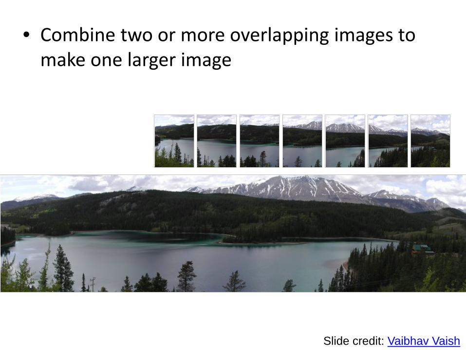
• Combine two or more overlapping images to make one larger image
Add example
Slide credit: Vaibhav Vaish
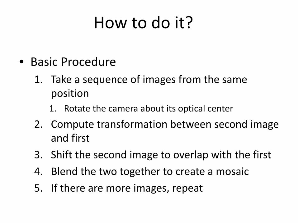
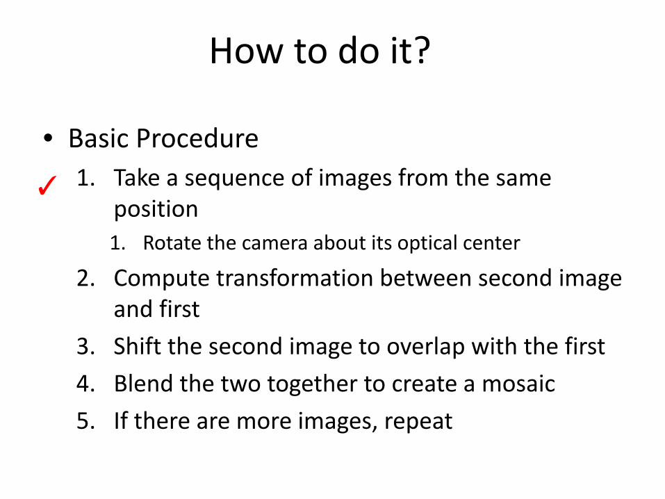
How to do it?
• Basic Procedure 1. Take a sequence of images from the same
position 1. Rotate the camera about its optical center
2. Compute transformation between second image and first
3. Shift the second image to overlap with the first 4. Blend the two together to create a mosaic 5. If there are more images, repeat
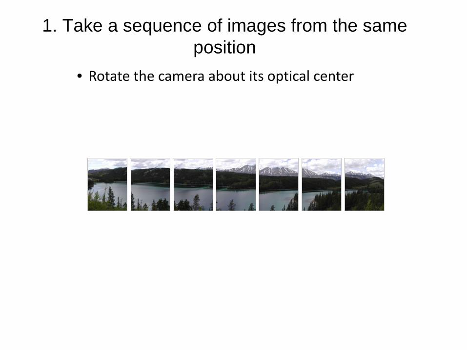
1. Take a sequence of images from the same position
• Rotate the camera about its optical center
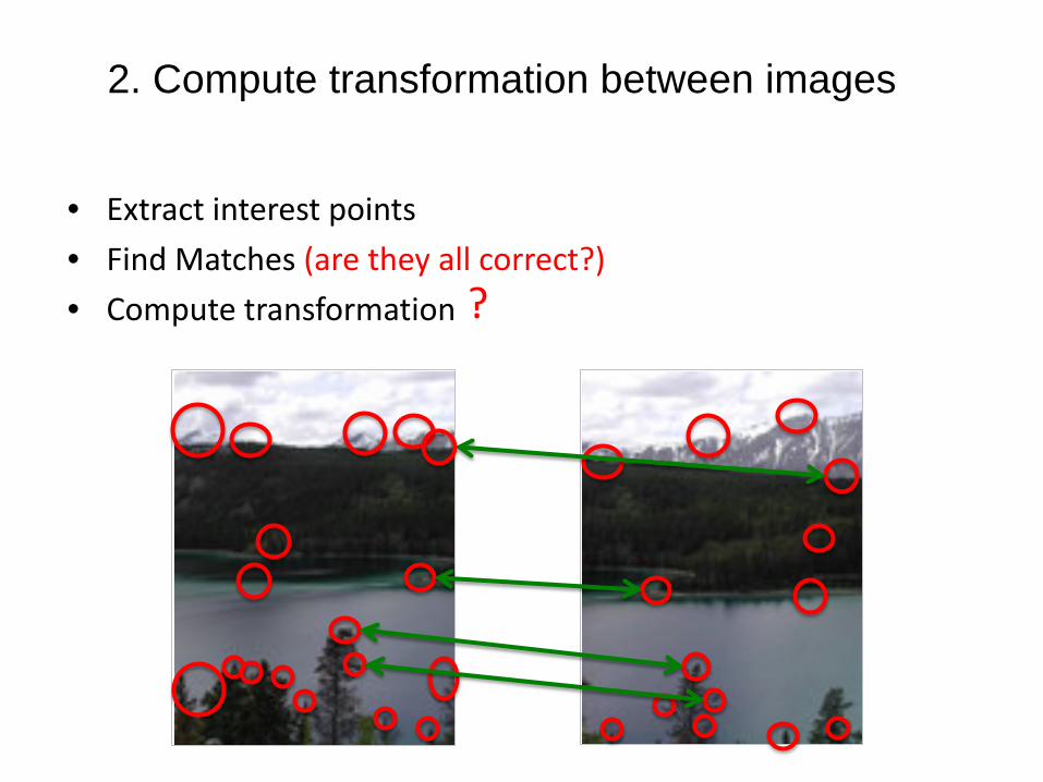
2. Compute transformation between images
• Extract interest points • Find Matches (are they all correct?) • Compute transformation ?
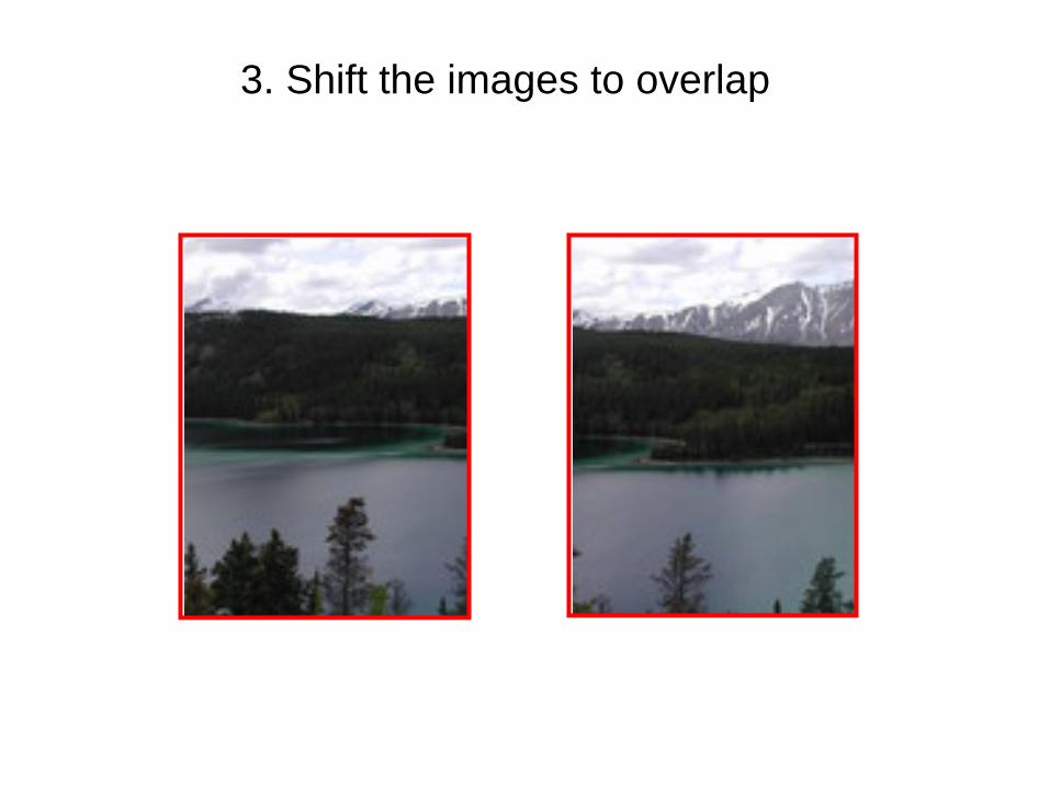
3. Shift the images to overlap
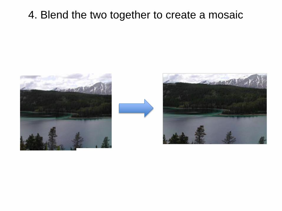
4. Blend the two together to create a mosaic

5. Repeat for all images
How to do it?
• Basic Procedure 1. Take a sequence of images from the same
position 1. Rotate the camera about its optical center
2. Compute transformation between second image and first
3. Shift the second image to overlap with the first 4. Blend the two together to create a mosaic 5. If there are more images, repeat
✓
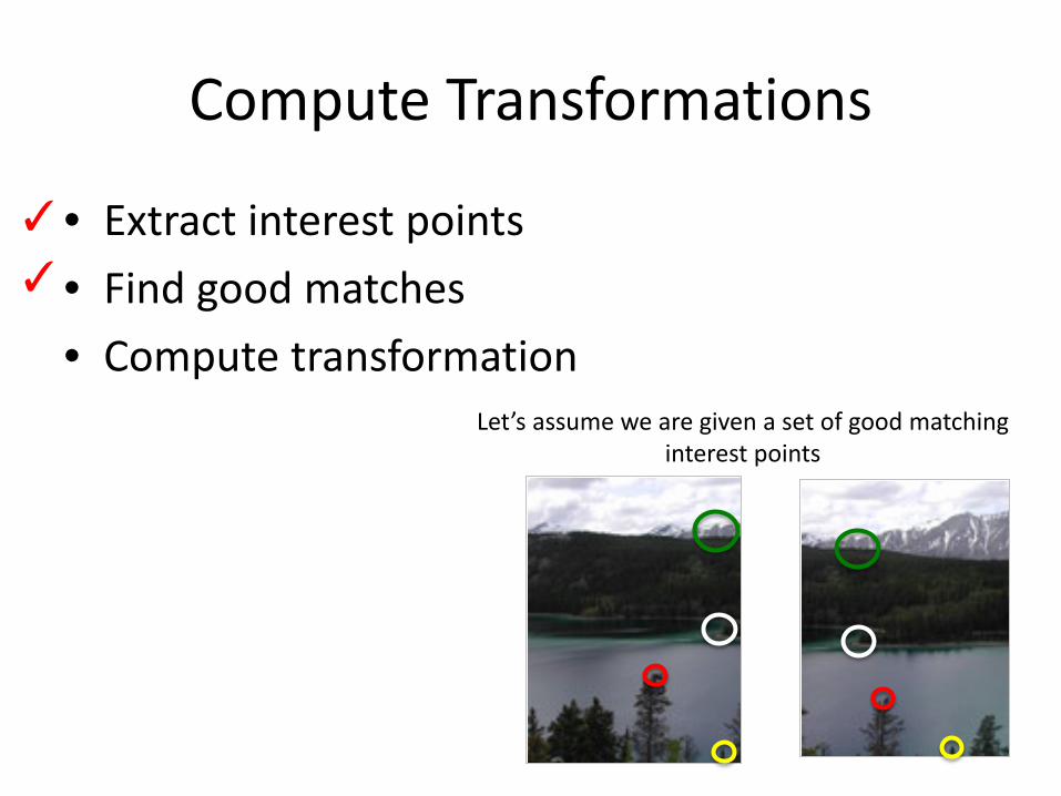
Compute Transformations
• Extract interest points • Find good matches • Compute transformation
✓
Let’s assume we are given a set of good matching interest points
✓

mosaic PP
Image reprojection
• The mosaic has a natural interpretation in 3D – The images are reprojected onto a common plane – The mosaic is formed on this plane
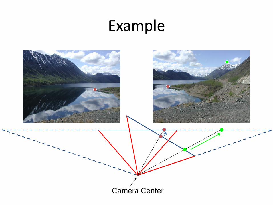
Example
Camera Center
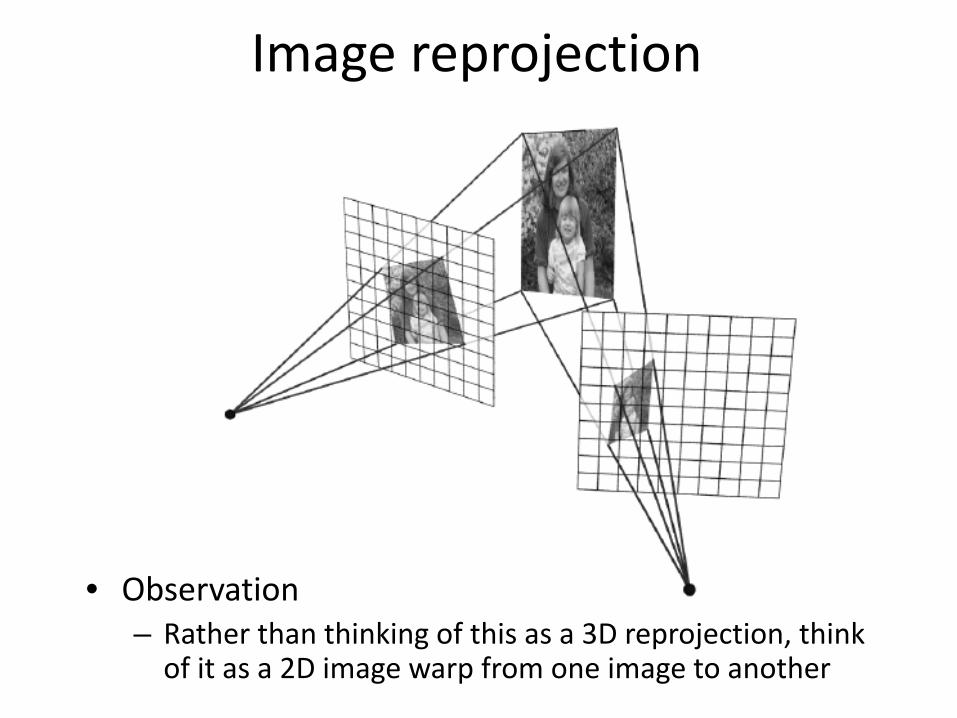
Image reprojection
• Observation – Rather than thinking of this as a 3D reprojection, think
of it as a 2D image warp from one image to another
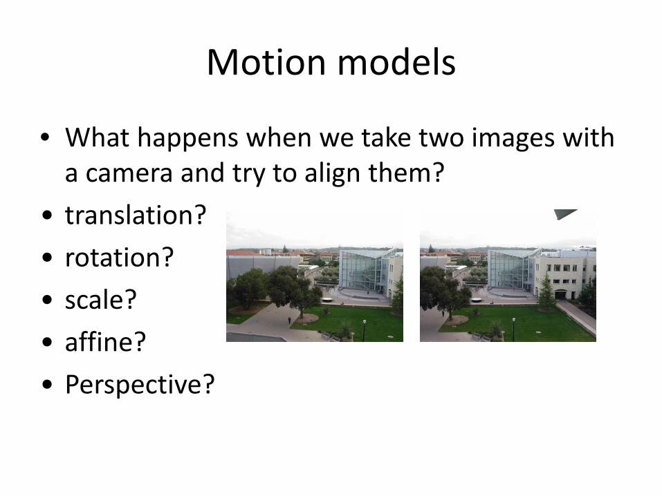
Motion models
• What happens when we take two images with a camera and try to align them?
• translation? • rotation? • scale? • affine? • Perspective?
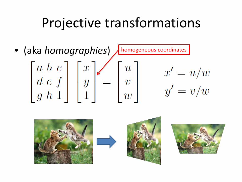
Projective transformations
• (aka homographies) homogeneous coordinates

Parametric (global) warping
• Examples of parametric warps:
translation rotation aspect
affine perspective
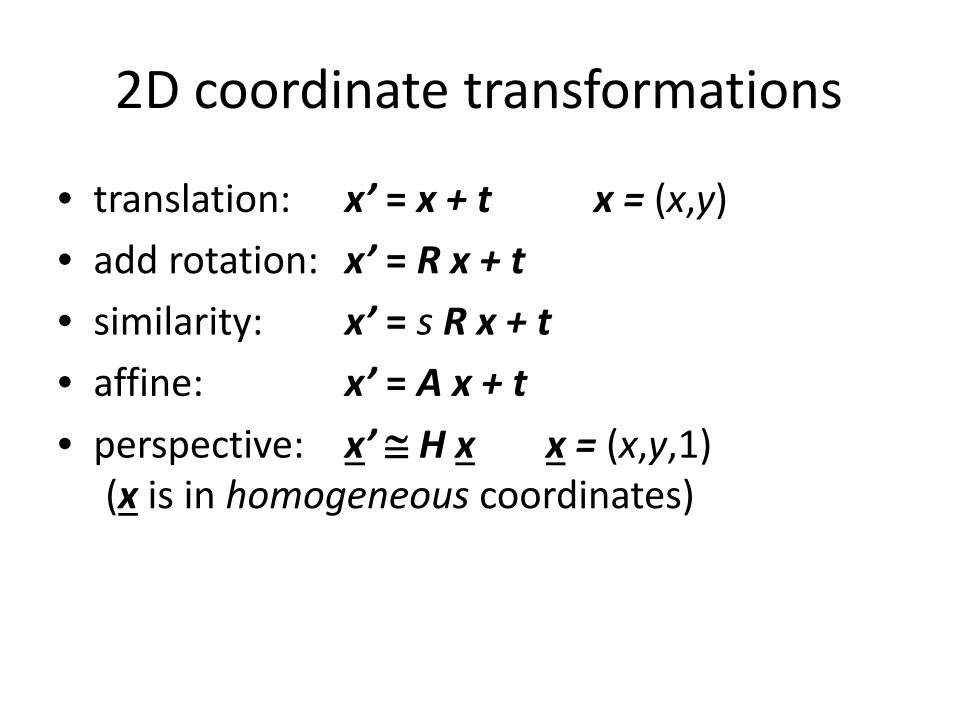
2D coordinate transformations
• translation: x’ = x + t x = (x,y) • add rotation: x’ = R x + t • similarity: x’ = s R x + t • affine: x’ = A x + t • perspective: x’ ≅ H x x = (x,y,1)
(x is in homogeneous coordinates)
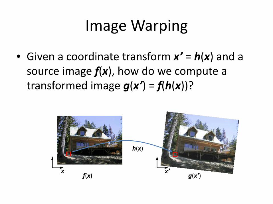
Image Warping
• Given a coordinate transform x’ = h(x) and a source image f(x), how do we compute a transformed image g(x’) = f(h(x))?
f(x) g(x’) x x’
h(x)
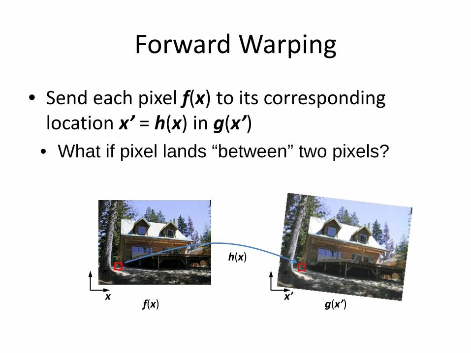
Forward Warping
• Send each pixel f(x) to its corresponding location x’ = h(x) in g(x’)
f(x) g(x’) x x’
h(x)
• What if pixel lands “between” two pixels?
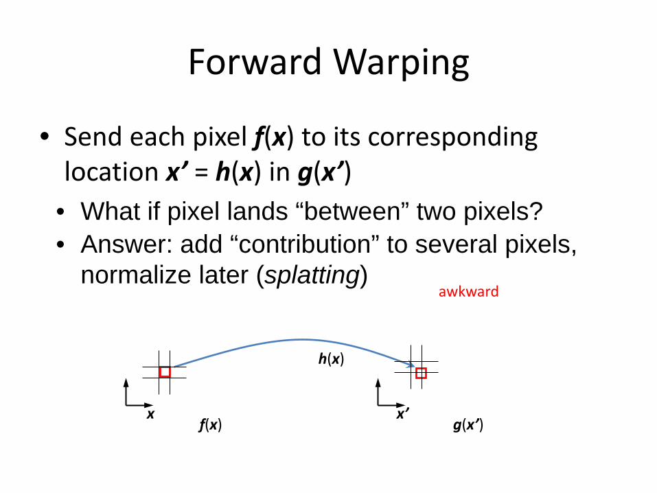
Forward Warping
• Send each pixel f(x) to its corresponding location x’ = h(x) in g(x’)
f(x) g(x’) x x’
h(x)
• What if pixel lands “between” two pixels? • Answer: add “contribution” to several pixels,
normalize later (splatting) awkward
Richard Szeliski Image Stitching 21
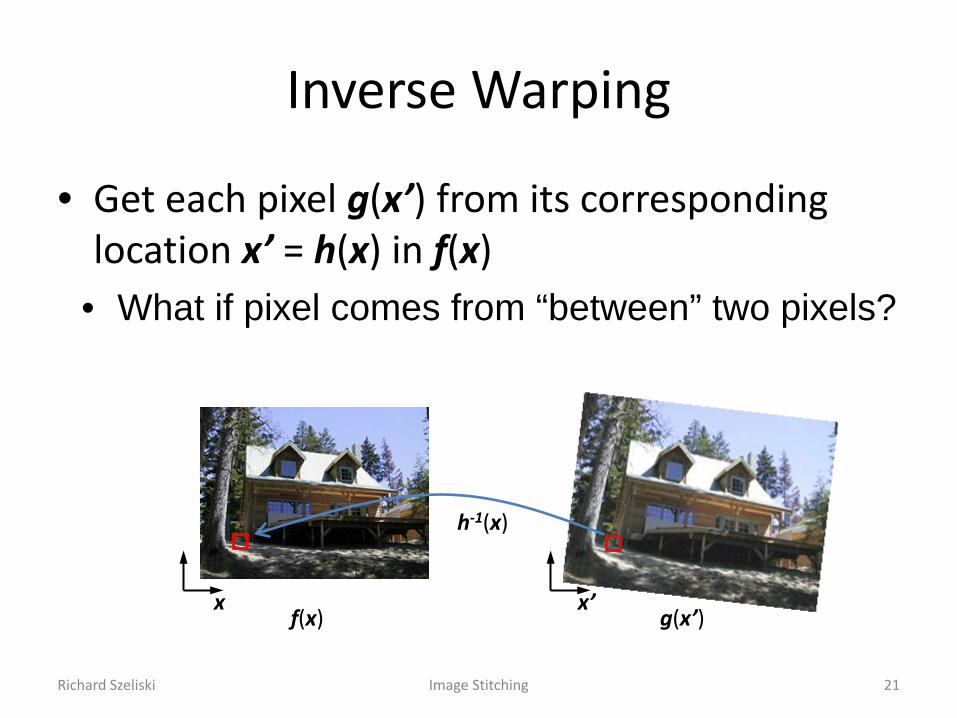
Inverse Warping
• Get each pixel g(x’) from its corresponding location x’ = h(x) in f(x)
f(x) g(x’) x x’
h-1(x)
• What if pixel comes from “between” two pixels?
Richard Szeliski Image Stitching 22
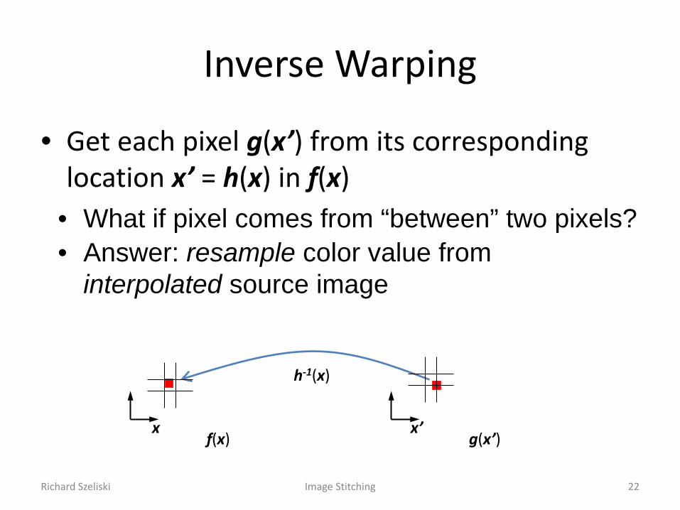
Inverse Warping
• Get each pixel g(x’) from its corresponding location x’ = h(x) in f(x)
• What if pixel comes from “between” two pixels? • Answer: resample color value from
interpolated source image
f(x) g(x’) x x’
h-1(x)
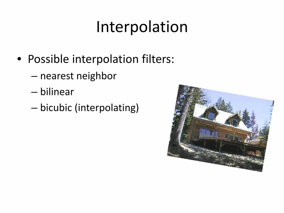
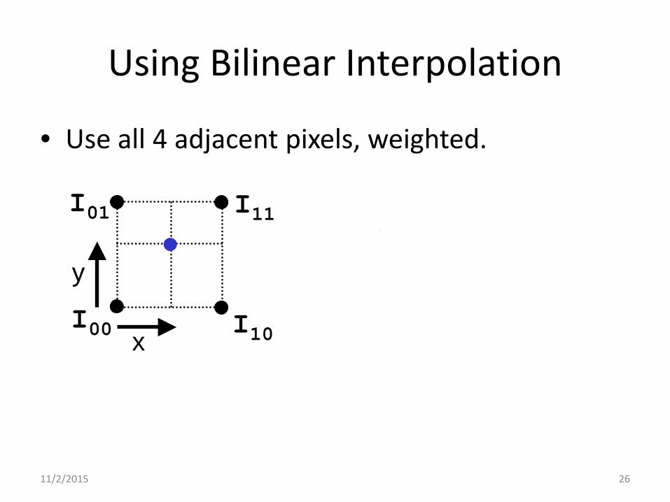
Interpolation
• Possible interpolation filters: – nearest neighbor – bilinear – bicubic (interpolating)
11/2/2015 24
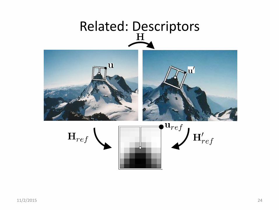
Related: Descriptors
11/2/2015 25
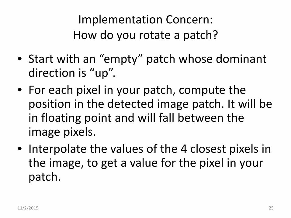
Implementation Concern: How do you rotate a patch?
• Start with an “empty” patch whose dominant direction is “up”.
• For each pixel in your patch, compute the position in the detected image patch. It will be in floating point and will fall between the image pixels.
• Interpolate the values of the 4 closest pixels in the image, to get a value for the pixel in your patch.
11/2/2015 26
Using Bilinear Interpolation
• Use all 4 adjacent pixels, weighted.
x
y
I00 I10
I01 I11
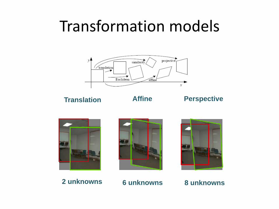
Transformation models
Translation
2 unknowns
Affine
6 unknowns
Perspective
8 unknowns

Finding the transformation
• Translation = 2 degrees of freedom • Similarity = 4 degrees of freedom • Affine = 6 degrees of freedom • Homography = 8 degrees of freedom
• How many corresponding points do we need
to solve?
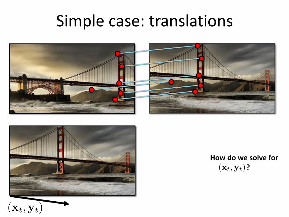
Simple case: translations
How do we solve for ?
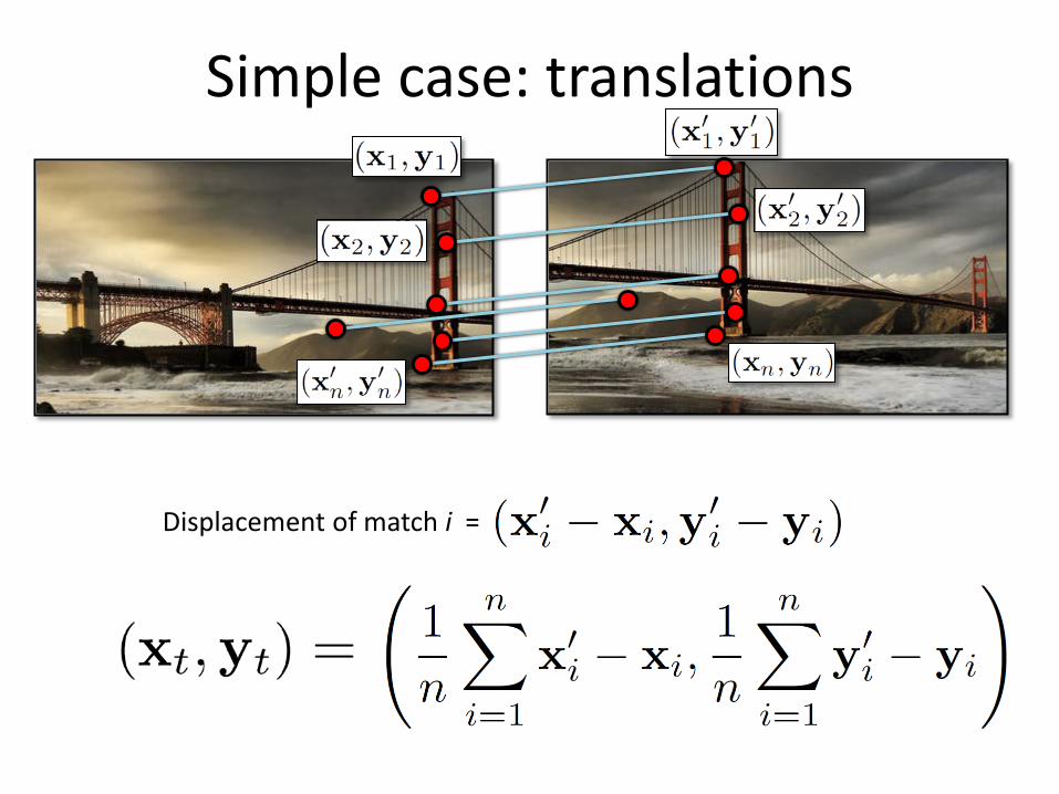
Mean displacement =
Simple case: translations
Displacement of match i =
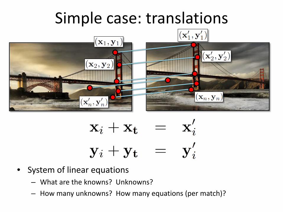
Simple case: translations
• System of linear equations – What are the knowns? Unknowns? – How many unknowns? How many equations (per match)?
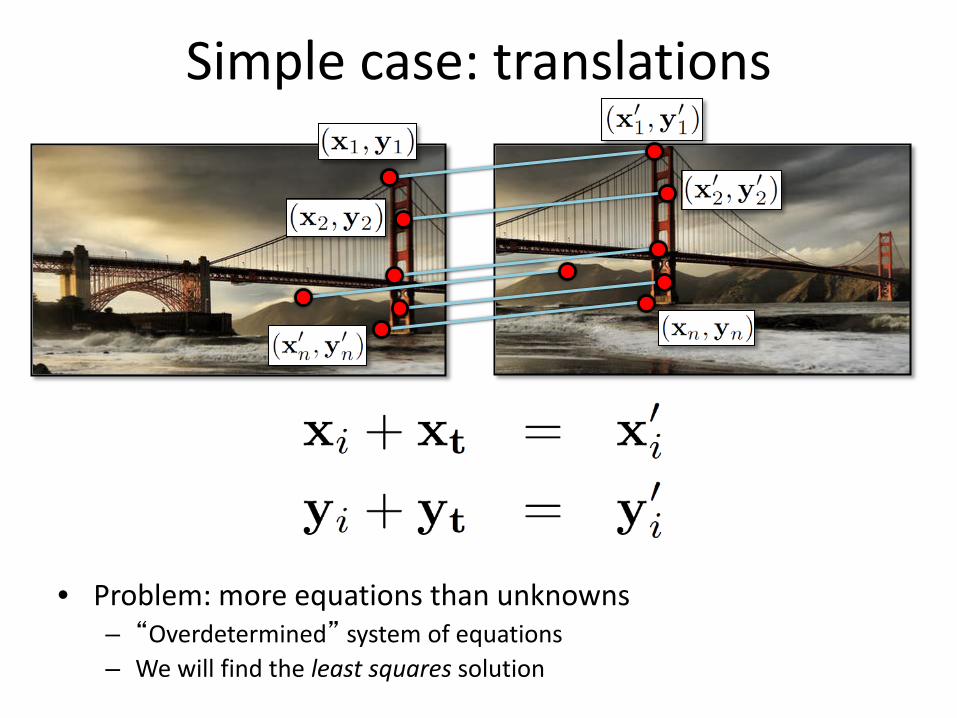
Simple case: translations
• Problem: more equations than unknowns – “Overdetermined” system of equations – We will find the least squares solution
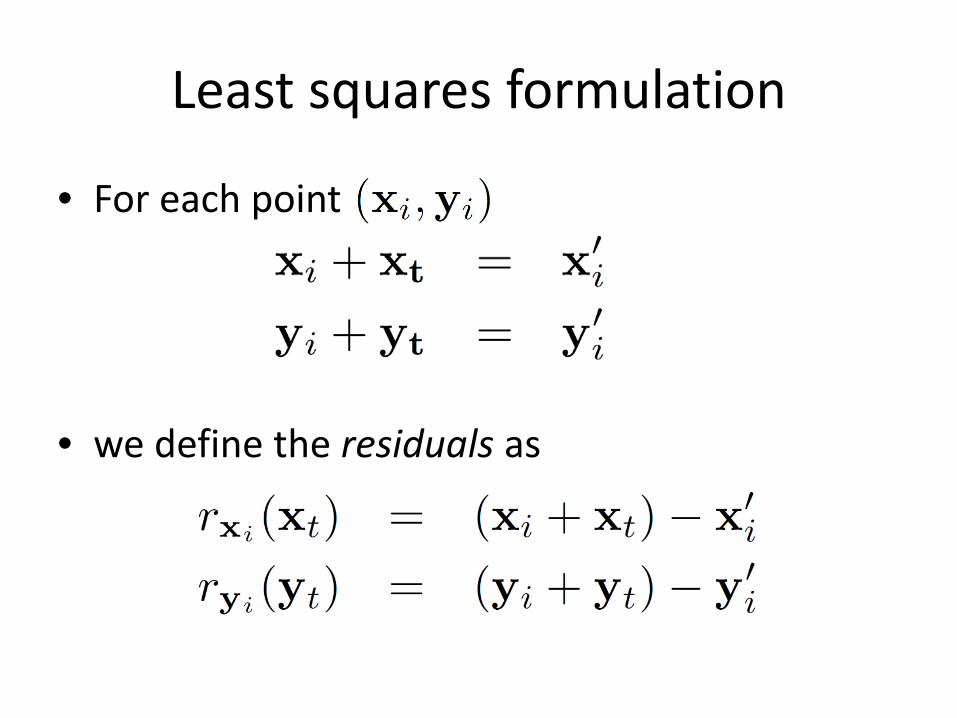
Least squares formulation
• For each point
• we define the residuals as
Least squares formulation
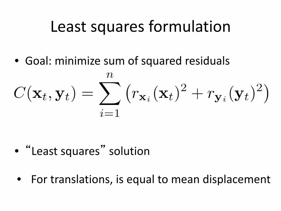
• Goal: minimize sum of squared residuals
• “Least squares” solution
• For translations, is equal to mean displacement
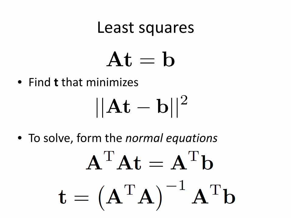
Least squares
• Find t that minimizes
• To solve, form the normal equations
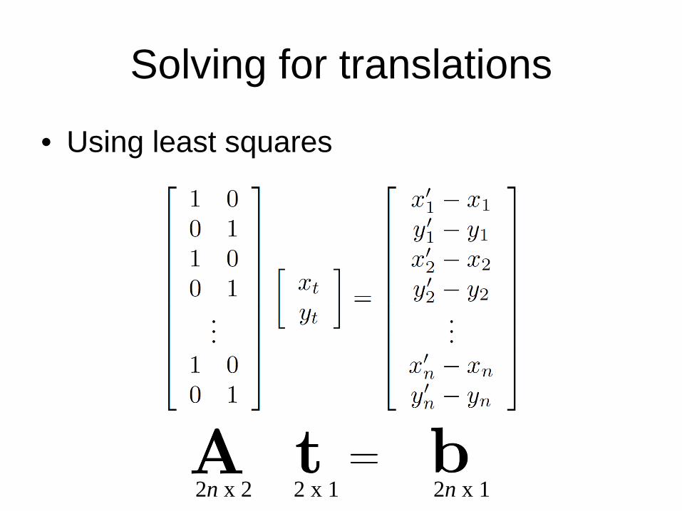
Solving for translations
• Using least squares
2n x 2 2 x 1 2n x 1
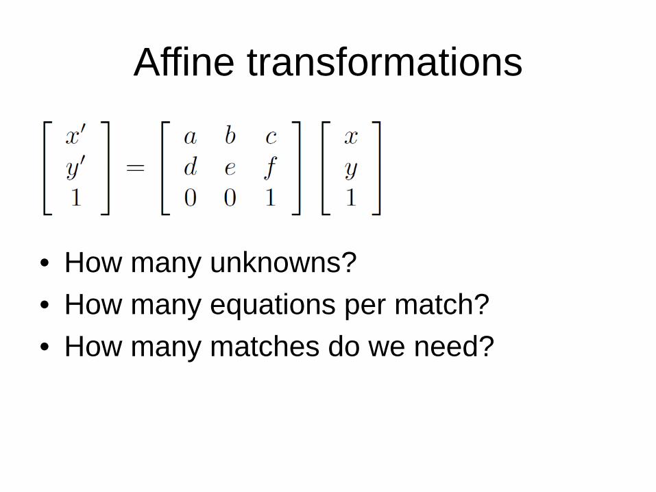
Affine transformations
• How many unknowns? • How many equations per match? • How many matches do we need?
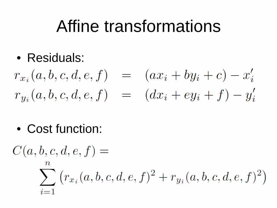
Affine transformations
• Residuals:
• Cost function:
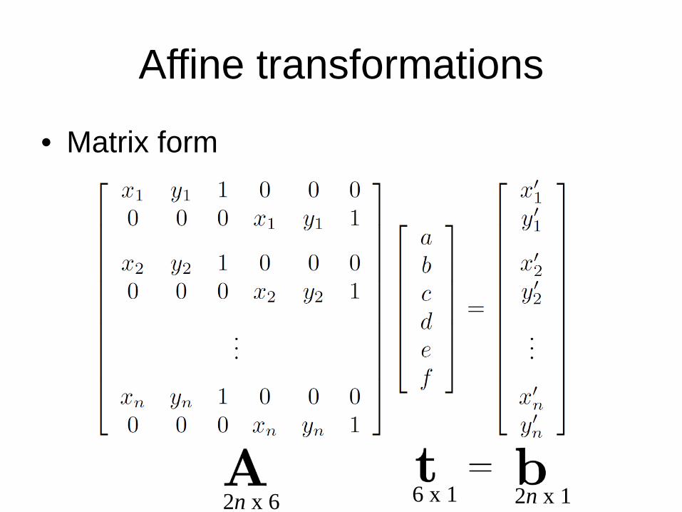
Affine transformations
• Matrix form
2n x 6 6 x 1 2n x 1
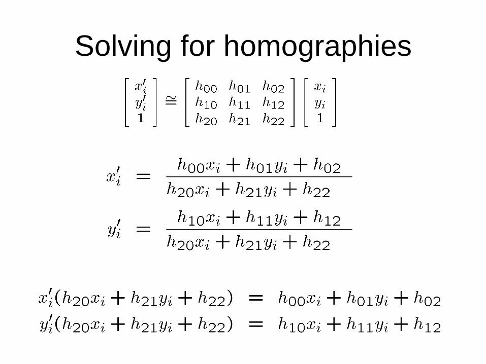
Solving for homographies

Solving for homographies

Direct Linear Transforms
Defines a least squares problem:
• Since is only defined up to scale, solve for unit vector • Solution: = eigenvector of with smallest eigenvalue • Works with 4 or more points
2n × 9 9 2n
Richard Szeliski Image Stitching 44
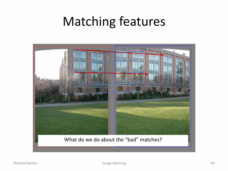
Matching features
What do we do about the “bad” matches?

Richard Szeliski Image Stitching 45
RAndom SAmple Consensus
Select one match, count inliers
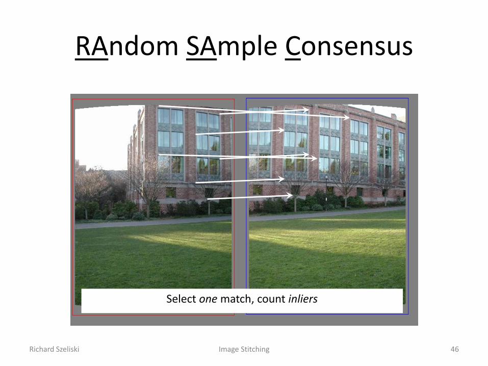
Richard Szeliski Image Stitching 46
RAndom SAmple Consensus
Select one match, count inliers
Richard Szeliski Image Stitching 47
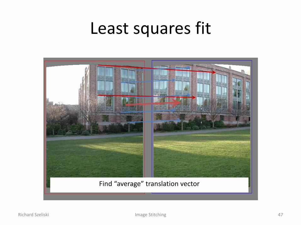
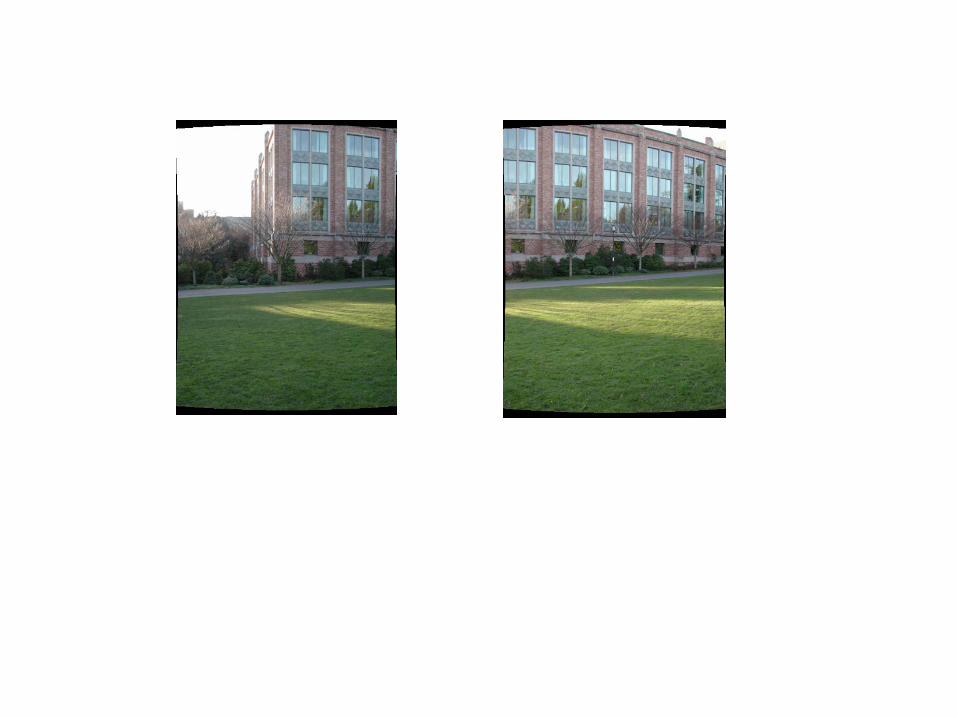
Least squares fit
Find “average” translation vector
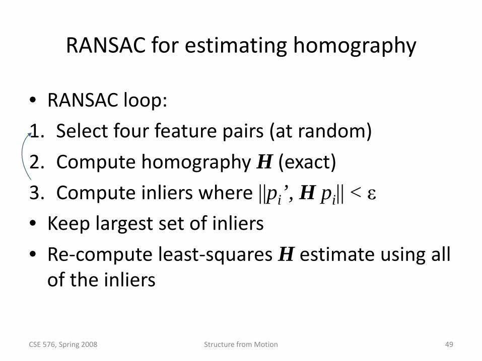
RANSAC for estimating homography
• RANSAC loop: 1. Select four feature pairs (at random) 2. Compute homography H (exact) 3. Compute inliers where ||pi’, H pi|| < ε • Keep largest set of inliers • Re-compute least-squares H estimate using all
of the inliers
CSE 576, Spring 2008 Structure from Motion 49
50
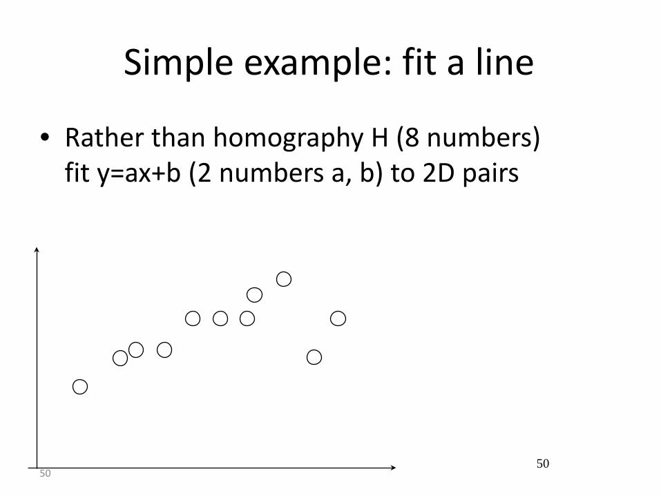
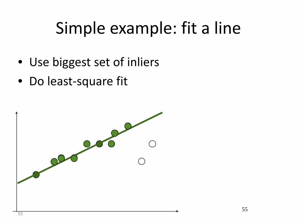
Simple example: fit a line
• Rather than homography H (8 numbers) fit y=ax+b (2 numbers a, b) to 2D pairs
50

51
Simple example: fit a line
• Pick 2 points • Fit line • Count inliers
51
3 inliers
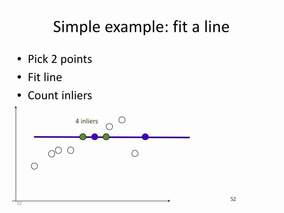
52
Simple example: fit a line
• Pick 2 points • Fit line • Count inliers
52
4 inliers
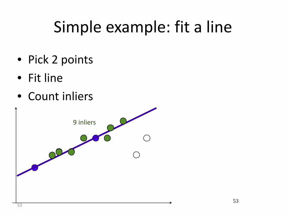
53
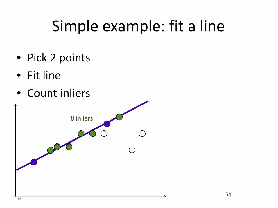
Simple example: fit a line
• Pick 2 points • Fit line • Count inliers
53
9 inliers
54
Simple example: fit a line
• Pick 2 points • Fit line • Count inliers
54
8 inliers
55
Simple example: fit a line
• Use biggest set of inliers • Do least-square fit
55

RANSAC
Red: rejected by 2nd nearest neighbor criterion Blue: Ransac outliers Yellow: inliers
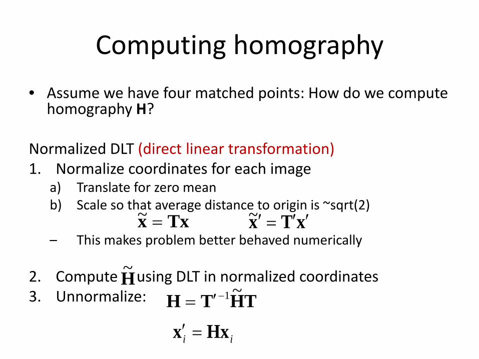
Computing homography • Assume we have four matched points: How do we compute
homography H? Normalized DLT (direct linear transformation) 1. Normalize coordinates for each image
a) Translate for zero mean b) Scale so that average distance to origin is ~sqrt(2)
– This makes problem better behaved numerically
2. Compute using DLT in normalized coordinates 3. Unnormalize:
Txx =~ xTx ′′=′~
THTH ~1−′=
ii Hxx =′
H~
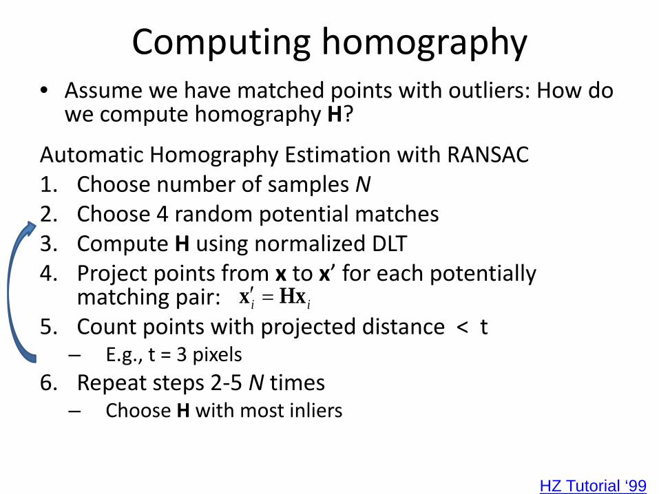
Computing homography • Assume we have matched points with outliers: How do
we compute homography H?
Automatic Homography Estimation with RANSAC 1. Choose number of samples N 2. Choose 4 random potential matches 3. Compute H using normalized DLT 4. Project points from x to x’ for each potentially
matching pair: 5. Count points with projected distance < t
– E.g., t = 3 pixels 6. Repeat steps 2-5 N times
– Choose H with most inliers
HZ Tutorial ‘99
ii Hxx =′
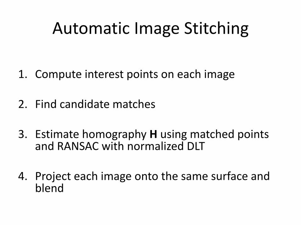
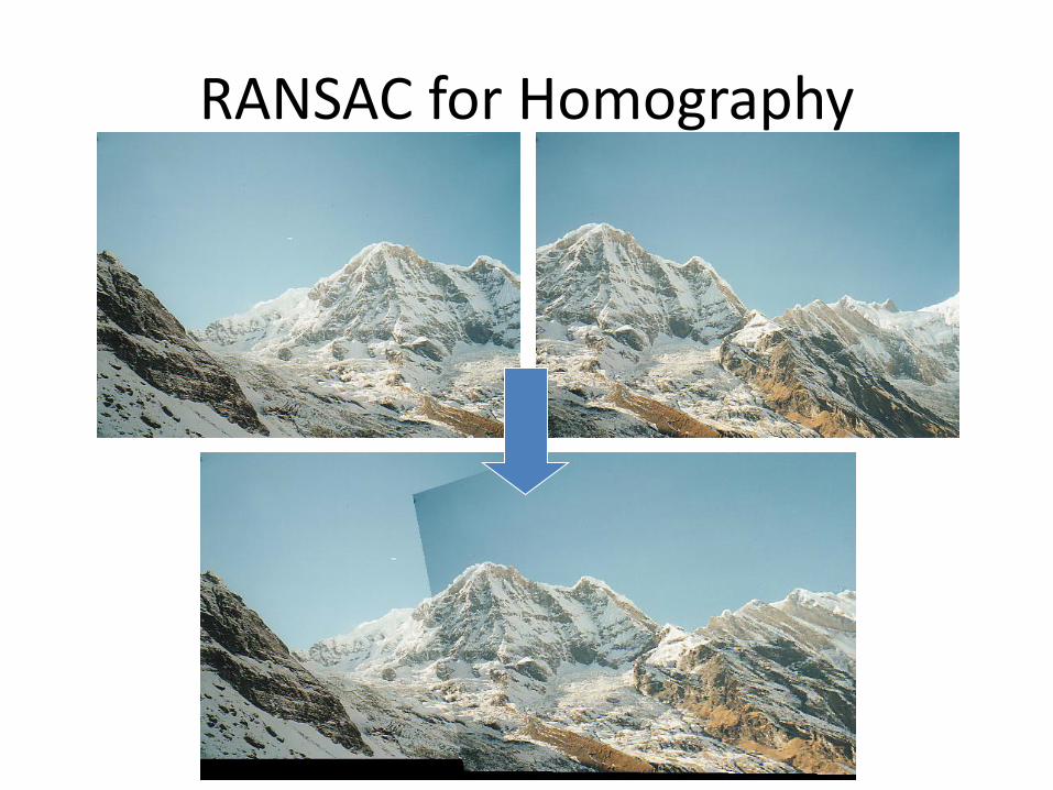
Automatic Image Stitching
1. Compute interest points on each image
2. Find candidate matches
3. Estimate homography H using matched points
and RANSAC with normalized DLT
4. Project each image onto the same surface and blend
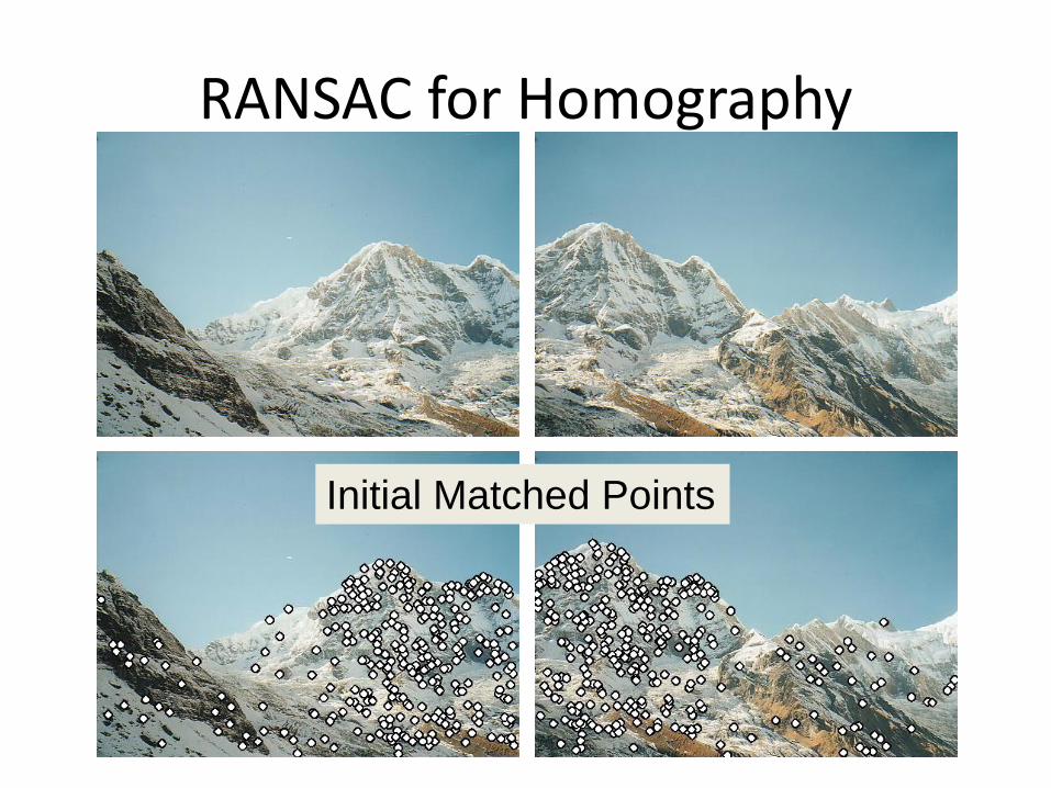
RANSAC for Homography
Initial Matched Points
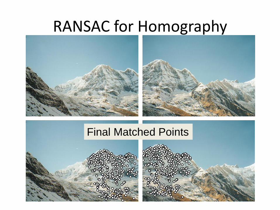
RANSAC for Homography
Final Matched Points
RANSAC for Homography

Image Blending
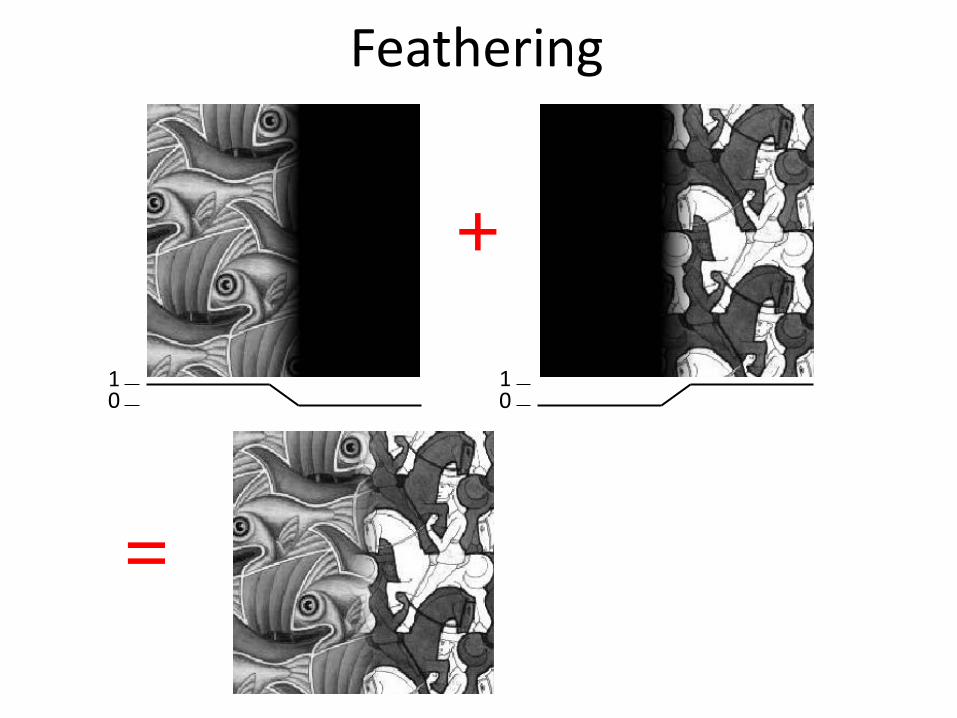
Feathering
0 1
0 1
+
=
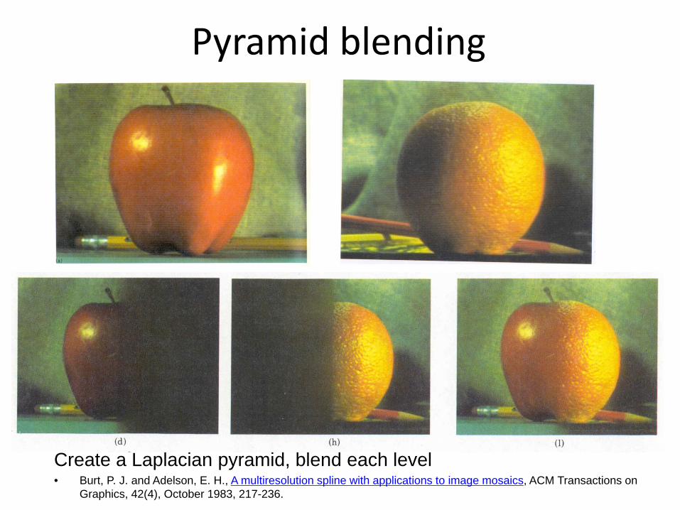
Pyramid blending
Create a Laplacian pyramid, blend each level • Burt, P. J. and Adelson, E. H., A multiresolution spline with applications to image mosaics, ACM Transactions on
Graphics, 42(4), October 1983, 217-236.
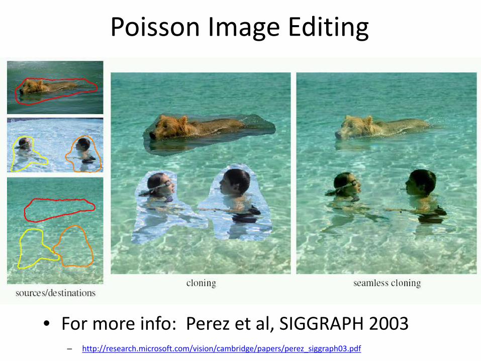
Poisson Image Editing
• For more info: Perez et al, SIGGRAPH 2003 – http://research.microsoft.com/vision/cambridge/papers/perez_siggraph03.pdf
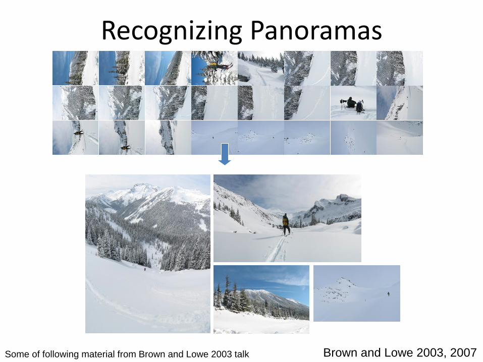
Recognizing Panoramas
Brown and Lowe 2003, 2007 Some of following material from Brown and Lowe 2003 talk
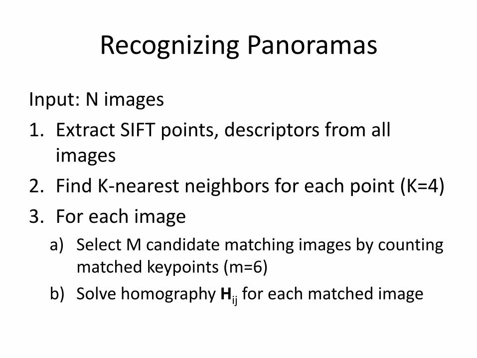
Recognizing Panoramas
Input: N images 1. Extract SIFT points, descriptors from all
images 2. Find K-nearest neighbors for each point (K=4) 3. For each image
a) Select M candidate matching images by counting matched keypoints (m=6)
b) Solve homography Hij for each matched image

Recognizing Panoramas
Input: N images 1. Extract SIFT points, descriptors from all
images 2. Find K-nearest neighbors for each point (K=4) 3. For each image
a) Select M candidate matching images by counting matched keypoints (m=6)
b) Solve homography Hij for each matched image c) Decide if match is valid (ni > 8 + 0.3 nf )
# inliers # keypoints in overlapping area
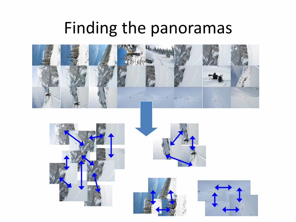
Recognizing Panoramas (cont.)
(now we have matched pairs of images) 4. Find connected components

Finding the panoramas
Finding the panoramas
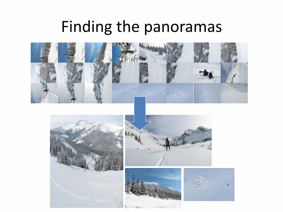
Finding the panoramas

Recognizing Panoramas (cont.)
(now we have matched pairs of images) 4. Find connected components 5. For each connected component
a) Solve for rotation and f b) Project to a surface (plane, cylinder, or sphere) c) Render with multiband blending