Image Modeling amp

SegmentationAly Farag and Asem Ali

Lecture 2

Intensity ModelldquoDensity Estimationrdquo

3

Intensity Models

The histogram of the whole image will represent the rate of occurrence for all the classes in the given empirical density

Each class can be described by the histogram of the occurrences of the gray levels within that class

Intensity models describe the statistical characteristics of each class in the given image marginal density

The objective of the intensity model is to estimate the marginal density for each class from the mixed normalized histogram of the occurrences of the gray levels

4

Density estimation can be studied under two primary umbrellas

Parametric methods and Nonparametric methods

Intensity Models

Nonparametric methods take a strong stance of letting the data (eg pixelsrsquo gray levels) represent themselves

One of the core methods that nonparametric density estimation approaches based on is the k-nearest neighbors (k-NN) method These approaches calculate the probability of a sample by combining the memorized responses for the k nearest neighbors of this sample in the training data

Nonparametric methods achieve good estimation for any input distribution as more data are observed

Flexible they can fit almost any data well No prior knowledge is required

However they apparently often have a high computational cost and have many parameters that need to be tuned

5

Nonparametric methods1

Based on the fact that the probability P that a given sample x falls within a region (window) of R is given by

This integral can be approximated either by the product of the value of p(x) with the areavolume of the region or by the ratio of number of samples fall within the region

if we observe a large number n of fish and count those whose length fall within the range defined by R then kn can be used as n estimate of P as nrarrinfin

1 Chapter 4 Duda R Hart P Stork D 2001 Pattern Classification 2nd edR John Wiley amp Sons

6

Nonparametric methods

In order to make sure that we get a good estimate of p(x) at each point we have to have lots of data points (instances) for any given R (or volume V) This can be done in two ways

1 We can fix V and take more and more samples in this volume Then knrarrP however we then estimate only an average of of p(x) not the p(x) itself because P can change in any region of nonzero volume

2 Alternatively we can fix n and make Vrarr0 so that p(x) is constant in that region However in practice we have a finite number of training data so as Vrarr0 V will be so small that it will eventually contain no samples k=01048774 p(x)=0 a useless result

Therefore Vrarr0 is not feasible and there will always be some variance in kn and hence some averaging in p(x) within the finite non-zero volume V

A compromise need to be found for V so that

It will be large enough to contain sufficient number of samples

It will be small enough to justify our assumption of p(x) be constant within the chosen volumeregion

7

Nonparametric methods

To make sure that kn is a good estimate of P and consequently pn(x) is a good estimate p(x) the following need to be satisfied

8

Nonparametric methods

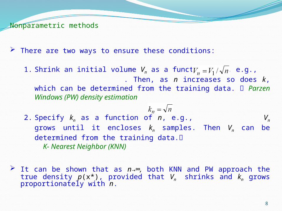
There are two ways to ensure these conditions

1 Shrink an initial volume Vn as a function of n eg Then as n increases so does k which can be determined from the training data 1048774 Parzen Windows (PW) density estimation

2 Specify kn as a function of n eg Vn grows until it encloses kn samples Then Vn can be determined from the training data1048774 K- Nearest Neighbor (KNN)

It can be shown that as nrarrinfin both KNN and PW approach the true density p(x) provided that Vn shrinks and kn grows proportionately with n

9

Parzen Windows

The number of samples falling into the specified region is obtained by the help of a windowing function hence the name Parzen windowsWe first assume that R is a d-dimensional hypercube of each side h whose volume is then V=(h)d1048774Then define a window function φ(u) called a kernel function to count the number of samples k that fall into R

10

Parzen Windows

ExampleGiven this image D = 1251123551515

For h=1 compute p(25)d = V = n = K = p(25) =

11

Parzen Windows

Now consider ϕ() as a general function typically a smooth and continuous function instead of a hypercube The general expression of p(x) remains unchanged

Then p(x) is an interpolation of ϕ()s where each ϕ() measures how far a given xi is from x

In practice xi are the training data points and we estimate p(x) by interpolating the contributions of each sample data point xi based on its distance from x the point at which we want to estimate the density The kernel function ϕ() provides the numerical value of this distance

If ϕ() is itself a distribution then p(x) will converge to p(x) as n increases A typical choice for ϕ() is the Gaussian

The density p(x) is then estimated simply by a superposition of Gaussians where each Gaussian is centered at the training data instances The parameter h is then the variance of the Gaussian

12

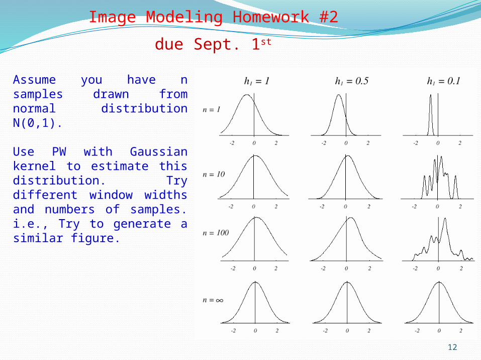
Assume you have n samples drawn from normal distribution N(01)

Use PW with Gaussian kernel to estimate this distribution Try different window widths and numbers of samples ie Try to generate a similar figure

Image Modeling Homework 2

due Sept 1st

K

jj

ii

cp

cpcP

1

)(

)()|(

x

xx

13

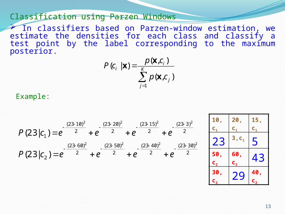
Classification using Parzen Windows In classifiers based on Parzen-window estimation we estimate the densities for each class and classify a test point by the label corresponding to the maximum posterior

10c1 20c1 15c1

23 3c1 550c2 60c2 4330c2 29 40c2

2

)3023(

2

)4023(

2

)5023(

2

)6023(

2

2

)323(

2

)1523(

2

)2023(

2

)1023(

1

2222

2222

)|23(

)|23(

eeeecP

eeeecP

Example

• Slide 1
• Slide 2
• Slide 3
• Slide 4
• Slide 5
• Slide 6
• Slide 7
• Slide 8
• Slide 9
• Slide 10
• Slide 11
• Slide 12
• Slide 13

Intensity ModelldquoDensity Estimationrdquo

3

Intensity Models

The histogram of the whole image will represent the rate of occurrence for all the classes in the given empirical density

Each class can be described by the histogram of the occurrences of the gray levels within that class

Intensity models describe the statistical characteristics of each class in the given image marginal density

The objective of the intensity model is to estimate the marginal density for each class from the mixed normalized histogram of the occurrences of the gray levels

4

Density estimation can be studied under two primary umbrellas

Parametric methods and Nonparametric methods

Intensity Models

Nonparametric methods take a strong stance of letting the data (eg pixelsrsquo gray levels) represent themselves

One of the core methods that nonparametric density estimation approaches based on is the k-nearest neighbors (k-NN) method These approaches calculate the probability of a sample by combining the memorized responses for the k nearest neighbors of this sample in the training data

Nonparametric methods achieve good estimation for any input distribution as more data are observed

Flexible they can fit almost any data well No prior knowledge is required

However they apparently often have a high computational cost and have many parameters that need to be tuned

5

Nonparametric methods1

Based on the fact that the probability P that a given sample x falls within a region (window) of R is given by

This integral can be approximated either by the product of the value of p(x) with the areavolume of the region or by the ratio of number of samples fall within the region

if we observe a large number n of fish and count those whose length fall within the range defined by R then kn can be used as n estimate of P as nrarrinfin

1 Chapter 4 Duda R Hart P Stork D 2001 Pattern Classification 2nd edR John Wiley amp Sons

6

Nonparametric methods

In order to make sure that we get a good estimate of p(x) at each point we have to have lots of data points (instances) for any given R (or volume V) This can be done in two ways

1 We can fix V and take more and more samples in this volume Then knrarrP however we then estimate only an average of of p(x) not the p(x) itself because P can change in any region of nonzero volume

2 Alternatively we can fix n and make Vrarr0 so that p(x) is constant in that region However in practice we have a finite number of training data so as Vrarr0 V will be so small that it will eventually contain no samples k=01048774 p(x)=0 a useless result

Therefore Vrarr0 is not feasible and there will always be some variance in kn and hence some averaging in p(x) within the finite non-zero volume V

A compromise need to be found for V so that

It will be large enough to contain sufficient number of samples

It will be small enough to justify our assumption of p(x) be constant within the chosen volumeregion

7

Nonparametric methods

To make sure that kn is a good estimate of P and consequently pn(x) is a good estimate p(x) the following need to be satisfied

8

Nonparametric methods

There are two ways to ensure these conditions

1 Shrink an initial volume Vn as a function of n eg Then as n increases so does k which can be determined from the training data 1048774 Parzen Windows (PW) density estimation

2 Specify kn as a function of n eg Vn grows until it encloses kn samples Then Vn can be determined from the training data1048774 K- Nearest Neighbor (KNN)

It can be shown that as nrarrinfin both KNN and PW approach the true density p(x) provided that Vn shrinks and kn grows proportionately with n

9

Parzen Windows

The number of samples falling into the specified region is obtained by the help of a windowing function hence the name Parzen windowsWe first assume that R is a d-dimensional hypercube of each side h whose volume is then V=(h)d1048774Then define a window function φ(u) called a kernel function to count the number of samples k that fall into R

10

Parzen Windows

ExampleGiven this image D = 1251123551515

For h=1 compute p(25)d = V = n = K = p(25) =

11

Parzen Windows

Now consider ϕ() as a general function typically a smooth and continuous function instead of a hypercube The general expression of p(x) remains unchanged

Then p(x) is an interpolation of ϕ()s where each ϕ() measures how far a given xi is from x

In practice xi are the training data points and we estimate p(x) by interpolating the contributions of each sample data point xi based on its distance from x the point at which we want to estimate the density The kernel function ϕ() provides the numerical value of this distance

If ϕ() is itself a distribution then p(x) will converge to p(x) as n increases A typical choice for ϕ() is the Gaussian

The density p(x) is then estimated simply by a superposition of Gaussians where each Gaussian is centered at the training data instances The parameter h is then the variance of the Gaussian

12

Assume you have n samples drawn from normal distribution N(01)

Use PW with Gaussian kernel to estimate this distribution Try different window widths and numbers of samples ie Try to generate a similar figure

Image Modeling Homework 2

due Sept 1st

K

jj

ii

cp

cpcP

1

)(

)()|(

x

xx

13

Classification using Parzen Windows In classifiers based on Parzen-window estimation we estimate the densities for each class and classify a test point by the label corresponding to the maximum posterior

10c1 20c1 15c1

23 3c1 550c2 60c2 4330c2 29 40c2

2

)3023(

2

)4023(

2

)5023(

2

)6023(

2

2

)323(

2

)1523(

2

)2023(

2

)1023(

1

2222

2222

)|23(

)|23(

eeeecP

eeeecP

Example

• Slide 1
• Slide 2
• Slide 3
• Slide 4
• Slide 5
• Slide 6
• Slide 7
• Slide 8
• Slide 9
• Slide 10
• Slide 11
• Slide 12
• Slide 13

3

Intensity Models

The histogram of the whole image will represent the rate of occurrence for all the classes in the given empirical density

Each class can be described by the histogram of the occurrences of the gray levels within that class

Intensity models describe the statistical characteristics of each class in the given image marginal density

The objective of the intensity model is to estimate the marginal density for each class from the mixed normalized histogram of the occurrences of the gray levels

4

Density estimation can be studied under two primary umbrellas

Parametric methods and Nonparametric methods

Intensity Models

Nonparametric methods take a strong stance of letting the data (eg pixelsrsquo gray levels) represent themselves

One of the core methods that nonparametric density estimation approaches based on is the k-nearest neighbors (k-NN) method These approaches calculate the probability of a sample by combining the memorized responses for the k nearest neighbors of this sample in the training data

Nonparametric methods achieve good estimation for any input distribution as more data are observed

Flexible they can fit almost any data well No prior knowledge is required

However they apparently often have a high computational cost and have many parameters that need to be tuned

5

Nonparametric methods1

Based on the fact that the probability P that a given sample x falls within a region (window) of R is given by

This integral can be approximated either by the product of the value of p(x) with the areavolume of the region or by the ratio of number of samples fall within the region

if we observe a large number n of fish and count those whose length fall within the range defined by R then kn can be used as n estimate of P as nrarrinfin

1 Chapter 4 Duda R Hart P Stork D 2001 Pattern Classification 2nd edR John Wiley amp Sons

6

Nonparametric methods

In order to make sure that we get a good estimate of p(x) at each point we have to have lots of data points (instances) for any given R (or volume V) This can be done in two ways

1 We can fix V and take more and more samples in this volume Then knrarrP however we then estimate only an average of of p(x) not the p(x) itself because P can change in any region of nonzero volume

2 Alternatively we can fix n and make Vrarr0 so that p(x) is constant in that region However in practice we have a finite number of training data so as Vrarr0 V will be so small that it will eventually contain no samples k=01048774 p(x)=0 a useless result

Therefore Vrarr0 is not feasible and there will always be some variance in kn and hence some averaging in p(x) within the finite non-zero volume V

A compromise need to be found for V so that

It will be large enough to contain sufficient number of samples

It will be small enough to justify our assumption of p(x) be constant within the chosen volumeregion

7

Nonparametric methods

To make sure that kn is a good estimate of P and consequently pn(x) is a good estimate p(x) the following need to be satisfied

8

Nonparametric methods

There are two ways to ensure these conditions

1 Shrink an initial volume Vn as a function of n eg Then as n increases so does k which can be determined from the training data 1048774 Parzen Windows (PW) density estimation

2 Specify kn as a function of n eg Vn grows until it encloses kn samples Then Vn can be determined from the training data1048774 K- Nearest Neighbor (KNN)

It can be shown that as nrarrinfin both KNN and PW approach the true density p(x) provided that Vn shrinks and kn grows proportionately with n

9

Parzen Windows

The number of samples falling into the specified region is obtained by the help of a windowing function hence the name Parzen windowsWe first assume that R is a d-dimensional hypercube of each side h whose volume is then V=(h)d1048774Then define a window function φ(u) called a kernel function to count the number of samples k that fall into R

10

Parzen Windows

ExampleGiven this image D = 1251123551515

For h=1 compute p(25)d = V = n = K = p(25) =

11

Parzen Windows

Now consider ϕ() as a general function typically a smooth and continuous function instead of a hypercube The general expression of p(x) remains unchanged

Then p(x) is an interpolation of ϕ()s where each ϕ() measures how far a given xi is from x

In practice xi are the training data points and we estimate p(x) by interpolating the contributions of each sample data point xi based on its distance from x the point at which we want to estimate the density The kernel function ϕ() provides the numerical value of this distance

If ϕ() is itself a distribution then p(x) will converge to p(x) as n increases A typical choice for ϕ() is the Gaussian

The density p(x) is then estimated simply by a superposition of Gaussians where each Gaussian is centered at the training data instances The parameter h is then the variance of the Gaussian

12

Assume you have n samples drawn from normal distribution N(01)

Use PW with Gaussian kernel to estimate this distribution Try different window widths and numbers of samples ie Try to generate a similar figure

Image Modeling Homework 2

due Sept 1st

K

jj

ii

cp

cpcP

1

)(

)()|(

x

xx

13

Classification using Parzen Windows In classifiers based on Parzen-window estimation we estimate the densities for each class and classify a test point by the label corresponding to the maximum posterior

10c1 20c1 15c1

23 3c1 550c2 60c2 4330c2 29 40c2

2

)3023(

2

)4023(

2

)5023(

2

)6023(

2

2

)323(

2

)1523(

2

)2023(

2

)1023(

1

2222

2222

)|23(

)|23(

eeeecP

eeeecP

Example

• Slide 1
• Slide 2
• Slide 3
• Slide 4
• Slide 5
• Slide 6
• Slide 7
• Slide 8
• Slide 9
• Slide 10
• Slide 11
• Slide 12
• Slide 13

4

Density estimation can be studied under two primary umbrellas

Parametric methods and Nonparametric methods

Intensity Models

Nonparametric methods take a strong stance of letting the data (eg pixelsrsquo gray levels) represent themselves

One of the core methods that nonparametric density estimation approaches based on is the k-nearest neighbors (k-NN) method These approaches calculate the probability of a sample by combining the memorized responses for the k nearest neighbors of this sample in the training data

Nonparametric methods achieve good estimation for any input distribution as more data are observed

Flexible they can fit almost any data well No prior knowledge is required

However they apparently often have a high computational cost and have many parameters that need to be tuned

5

Nonparametric methods1

Based on the fact that the probability P that a given sample x falls within a region (window) of R is given by

This integral can be approximated either by the product of the value of p(x) with the areavolume of the region or by the ratio of number of samples fall within the region

if we observe a large number n of fish and count those whose length fall within the range defined by R then kn can be used as n estimate of P as nrarrinfin

1 Chapter 4 Duda R Hart P Stork D 2001 Pattern Classification 2nd edR John Wiley amp Sons

6

Nonparametric methods

In order to make sure that we get a good estimate of p(x) at each point we have to have lots of data points (instances) for any given R (or volume V) This can be done in two ways

1 We can fix V and take more and more samples in this volume Then knrarrP however we then estimate only an average of of p(x) not the p(x) itself because P can change in any region of nonzero volume

2 Alternatively we can fix n and make Vrarr0 so that p(x) is constant in that region However in practice we have a finite number of training data so as Vrarr0 V will be so small that it will eventually contain no samples k=01048774 p(x)=0 a useless result

Therefore Vrarr0 is not feasible and there will always be some variance in kn and hence some averaging in p(x) within the finite non-zero volume V

A compromise need to be found for V so that

It will be large enough to contain sufficient number of samples

It will be small enough to justify our assumption of p(x) be constant within the chosen volumeregion

7

Nonparametric methods

To make sure that kn is a good estimate of P and consequently pn(x) is a good estimate p(x) the following need to be satisfied

8

Nonparametric methods

There are two ways to ensure these conditions

1 Shrink an initial volume Vn as a function of n eg Then as n increases so does k which can be determined from the training data 1048774 Parzen Windows (PW) density estimation

2 Specify kn as a function of n eg Vn grows until it encloses kn samples Then Vn can be determined from the training data1048774 K- Nearest Neighbor (KNN)

It can be shown that as nrarrinfin both KNN and PW approach the true density p(x) provided that Vn shrinks and kn grows proportionately with n

9

Parzen Windows

The number of samples falling into the specified region is obtained by the help of a windowing function hence the name Parzen windowsWe first assume that R is a d-dimensional hypercube of each side h whose volume is then V=(h)d1048774Then define a window function φ(u) called a kernel function to count the number of samples k that fall into R

10

Parzen Windows

ExampleGiven this image D = 1251123551515

For h=1 compute p(25)d = V = n = K = p(25) =

11

Parzen Windows

Now consider ϕ() as a general function typically a smooth and continuous function instead of a hypercube The general expression of p(x) remains unchanged

Then p(x) is an interpolation of ϕ()s where each ϕ() measures how far a given xi is from x

In practice xi are the training data points and we estimate p(x) by interpolating the contributions of each sample data point xi based on its distance from x the point at which we want to estimate the density The kernel function ϕ() provides the numerical value of this distance

If ϕ() is itself a distribution then p(x) will converge to p(x) as n increases A typical choice for ϕ() is the Gaussian

The density p(x) is then estimated simply by a superposition of Gaussians where each Gaussian is centered at the training data instances The parameter h is then the variance of the Gaussian

12

Assume you have n samples drawn from normal distribution N(01)

Use PW with Gaussian kernel to estimate this distribution Try different window widths and numbers of samples ie Try to generate a similar figure

Image Modeling Homework 2

due Sept 1st

K

jj

ii

cp

cpcP

1

)(

)()|(

x

xx

13

Classification using Parzen Windows In classifiers based on Parzen-window estimation we estimate the densities for each class and classify a test point by the label corresponding to the maximum posterior

10c1 20c1 15c1

23 3c1 550c2 60c2 4330c2 29 40c2

2

)3023(

2

)4023(

2

)5023(

2

)6023(

2

2

)323(

2

)1523(

2

)2023(

2

)1023(

1

2222

2222

)|23(

)|23(

eeeecP

eeeecP

Example

• Slide 1
• Slide 2
• Slide 3
• Slide 4
• Slide 5
• Slide 6
• Slide 7
• Slide 8
• Slide 9
• Slide 10
• Slide 11
• Slide 12
• Slide 13

5

Nonparametric methods1

Based on the fact that the probability P that a given sample x falls within a region (window) of R is given by

This integral can be approximated either by the product of the value of p(x) with the areavolume of the region or by the ratio of number of samples fall within the region

if we observe a large number n of fish and count those whose length fall within the range defined by R then kn can be used as n estimate of P as nrarrinfin

1 Chapter 4 Duda R Hart P Stork D 2001 Pattern Classification 2nd edR John Wiley amp Sons

6

Nonparametric methods

In order to make sure that we get a good estimate of p(x) at each point we have to have lots of data points (instances) for any given R (or volume V) This can be done in two ways

1 We can fix V and take more and more samples in this volume Then knrarrP however we then estimate only an average of of p(x) not the p(x) itself because P can change in any region of nonzero volume

2 Alternatively we can fix n and make Vrarr0 so that p(x) is constant in that region However in practice we have a finite number of training data so as Vrarr0 V will be so small that it will eventually contain no samples k=01048774 p(x)=0 a useless result

Therefore Vrarr0 is not feasible and there will always be some variance in kn and hence some averaging in p(x) within the finite non-zero volume V

A compromise need to be found for V so that

It will be large enough to contain sufficient number of samples

It will be small enough to justify our assumption of p(x) be constant within the chosen volumeregion

7

Nonparametric methods

To make sure that kn is a good estimate of P and consequently pn(x) is a good estimate p(x) the following need to be satisfied

8

Nonparametric methods

There are two ways to ensure these conditions

1 Shrink an initial volume Vn as a function of n eg Then as n increases so does k which can be determined from the training data 1048774 Parzen Windows (PW) density estimation

2 Specify kn as a function of n eg Vn grows until it encloses kn samples Then Vn can be determined from the training data1048774 K- Nearest Neighbor (KNN)

It can be shown that as nrarrinfin both KNN and PW approach the true density p(x) provided that Vn shrinks and kn grows proportionately with n

9

Parzen Windows

The number of samples falling into the specified region is obtained by the help of a windowing function hence the name Parzen windowsWe first assume that R is a d-dimensional hypercube of each side h whose volume is then V=(h)d1048774Then define a window function φ(u) called a kernel function to count the number of samples k that fall into R

10

Parzen Windows

ExampleGiven this image D = 1251123551515

For h=1 compute p(25)d = V = n = K = p(25) =

11

Parzen Windows

Now consider ϕ() as a general function typically a smooth and continuous function instead of a hypercube The general expression of p(x) remains unchanged

Then p(x) is an interpolation of ϕ()s where each ϕ() measures how far a given xi is from x

In practice xi are the training data points and we estimate p(x) by interpolating the contributions of each sample data point xi based on its distance from x the point at which we want to estimate the density The kernel function ϕ() provides the numerical value of this distance

If ϕ() is itself a distribution then p(x) will converge to p(x) as n increases A typical choice for ϕ() is the Gaussian

The density p(x) is then estimated simply by a superposition of Gaussians where each Gaussian is centered at the training data instances The parameter h is then the variance of the Gaussian

12

Assume you have n samples drawn from normal distribution N(01)

Use PW with Gaussian kernel to estimate this distribution Try different window widths and numbers of samples ie Try to generate a similar figure

Image Modeling Homework 2

due Sept 1st

K

jj

ii

cp

cpcP

1

)(

)()|(

x

xx

13

Classification using Parzen Windows In classifiers based on Parzen-window estimation we estimate the densities for each class and classify a test point by the label corresponding to the maximum posterior

10c1 20c1 15c1

23 3c1 550c2 60c2 4330c2 29 40c2

2

)3023(

2

)4023(

2

)5023(

2

)6023(

2

2

)323(

2

)1523(

2

)2023(

2

)1023(

1

2222

2222

)|23(

)|23(

eeeecP

eeeecP

Example

• Slide 1
• Slide 2
• Slide 3
• Slide 4
• Slide 5
• Slide 6
• Slide 7
• Slide 8
• Slide 9
• Slide 10
• Slide 11
• Slide 12
• Slide 13

6

Nonparametric methods

In order to make sure that we get a good estimate of p(x) at each point we have to have lots of data points (instances) for any given R (or volume V) This can be done in two ways

1 We can fix V and take more and more samples in this volume Then knrarrP however we then estimate only an average of of p(x) not the p(x) itself because P can change in any region of nonzero volume

2 Alternatively we can fix n and make Vrarr0 so that p(x) is constant in that region However in practice we have a finite number of training data so as Vrarr0 V will be so small that it will eventually contain no samples k=01048774 p(x)=0 a useless result

Therefore Vrarr0 is not feasible and there will always be some variance in kn and hence some averaging in p(x) within the finite non-zero volume V

A compromise need to be found for V so that

It will be large enough to contain sufficient number of samples

It will be small enough to justify our assumption of p(x) be constant within the chosen volumeregion

7

Nonparametric methods

To make sure that kn is a good estimate of P and consequently pn(x) is a good estimate p(x) the following need to be satisfied

8

Nonparametric methods

There are two ways to ensure these conditions

1 Shrink an initial volume Vn as a function of n eg Then as n increases so does k which can be determined from the training data 1048774 Parzen Windows (PW) density estimation

2 Specify kn as a function of n eg Vn grows until it encloses kn samples Then Vn can be determined from the training data1048774 K- Nearest Neighbor (KNN)

It can be shown that as nrarrinfin both KNN and PW approach the true density p(x) provided that Vn shrinks and kn grows proportionately with n

9

Parzen Windows

The number of samples falling into the specified region is obtained by the help of a windowing function hence the name Parzen windowsWe first assume that R is a d-dimensional hypercube of each side h whose volume is then V=(h)d1048774Then define a window function φ(u) called a kernel function to count the number of samples k that fall into R

10

Parzen Windows

ExampleGiven this image D = 1251123551515

For h=1 compute p(25)d = V = n = K = p(25) =

11

Parzen Windows

Now consider ϕ() as a general function typically a smooth and continuous function instead of a hypercube The general expression of p(x) remains unchanged

Then p(x) is an interpolation of ϕ()s where each ϕ() measures how far a given xi is from x

In practice xi are the training data points and we estimate p(x) by interpolating the contributions of each sample data point xi based on its distance from x the point at which we want to estimate the density The kernel function ϕ() provides the numerical value of this distance

If ϕ() is itself a distribution then p(x) will converge to p(x) as n increases A typical choice for ϕ() is the Gaussian

The density p(x) is then estimated simply by a superposition of Gaussians where each Gaussian is centered at the training data instances The parameter h is then the variance of the Gaussian

12

Assume you have n samples drawn from normal distribution N(01)

Use PW with Gaussian kernel to estimate this distribution Try different window widths and numbers of samples ie Try to generate a similar figure

Image Modeling Homework 2

due Sept 1st

K

jj

ii

cp

cpcP

1

)(

)()|(

x

xx

13

Classification using Parzen Windows In classifiers based on Parzen-window estimation we estimate the densities for each class and classify a test point by the label corresponding to the maximum posterior

10c1 20c1 15c1

23 3c1 550c2 60c2 4330c2 29 40c2

2

)3023(

2

)4023(

2

)5023(

2

)6023(

2

2

)323(

2

)1523(

2

)2023(

2

)1023(

1

2222

2222

)|23(

)|23(

eeeecP

eeeecP

Example

• Slide 1
• Slide 2
• Slide 3
• Slide 4
• Slide 5
• Slide 6
• Slide 7
• Slide 8
• Slide 9
• Slide 10
• Slide 11
• Slide 12
• Slide 13

7

Nonparametric methods

To make sure that kn is a good estimate of P and consequently pn(x) is a good estimate p(x) the following need to be satisfied

8

Nonparametric methods

There are two ways to ensure these conditions

1 Shrink an initial volume Vn as a function of n eg Then as n increases so does k which can be determined from the training data 1048774 Parzen Windows (PW) density estimation

2 Specify kn as a function of n eg Vn grows until it encloses kn samples Then Vn can be determined from the training data1048774 K- Nearest Neighbor (KNN)

It can be shown that as nrarrinfin both KNN and PW approach the true density p(x) provided that Vn shrinks and kn grows proportionately with n

9

Parzen Windows

The number of samples falling into the specified region is obtained by the help of a windowing function hence the name Parzen windowsWe first assume that R is a d-dimensional hypercube of each side h whose volume is then V=(h)d1048774Then define a window function φ(u) called a kernel function to count the number of samples k that fall into R

10

Parzen Windows

ExampleGiven this image D = 1251123551515

For h=1 compute p(25)d = V = n = K = p(25) =

11

Parzen Windows

Now consider ϕ() as a general function typically a smooth and continuous function instead of a hypercube The general expression of p(x) remains unchanged

Then p(x) is an interpolation of ϕ()s where each ϕ() measures how far a given xi is from x

In practice xi are the training data points and we estimate p(x) by interpolating the contributions of each sample data point xi based on its distance from x the point at which we want to estimate the density The kernel function ϕ() provides the numerical value of this distance

If ϕ() is itself a distribution then p(x) will converge to p(x) as n increases A typical choice for ϕ() is the Gaussian

The density p(x) is then estimated simply by a superposition of Gaussians where each Gaussian is centered at the training data instances The parameter h is then the variance of the Gaussian

12

Assume you have n samples drawn from normal distribution N(01)

Use PW with Gaussian kernel to estimate this distribution Try different window widths and numbers of samples ie Try to generate a similar figure

Image Modeling Homework 2

due Sept 1st

K

jj

ii

cp

cpcP

1

)(

)()|(

x

xx

13

Classification using Parzen Windows In classifiers based on Parzen-window estimation we estimate the densities for each class and classify a test point by the label corresponding to the maximum posterior

10c1 20c1 15c1

23 3c1 550c2 60c2 4330c2 29 40c2

2

)3023(

2

)4023(

2

)5023(

2

)6023(

2

2

)323(

2

)1523(

2

)2023(

2

)1023(

1

2222

2222

)|23(

)|23(

eeeecP

eeeecP

Example

• Slide 1
• Slide 2
• Slide 3
• Slide 4
• Slide 5
• Slide 6
• Slide 7
• Slide 8
• Slide 9
• Slide 10
• Slide 11
• Slide 12
• Slide 13

8

Nonparametric methods

There are two ways to ensure these conditions

1 Shrink an initial volume Vn as a function of n eg Then as n increases so does k which can be determined from the training data 1048774 Parzen Windows (PW) density estimation

2 Specify kn as a function of n eg Vn grows until it encloses kn samples Then Vn can be determined from the training data1048774 K- Nearest Neighbor (KNN)

It can be shown that as nrarrinfin both KNN and PW approach the true density p(x) provided that Vn shrinks and kn grows proportionately with n

9

Parzen Windows

The number of samples falling into the specified region is obtained by the help of a windowing function hence the name Parzen windowsWe first assume that R is a d-dimensional hypercube of each side h whose volume is then V=(h)d1048774Then define a window function φ(u) called a kernel function to count the number of samples k that fall into R

10

Parzen Windows

ExampleGiven this image D = 1251123551515

For h=1 compute p(25)d = V = n = K = p(25) =

11

Parzen Windows

Now consider ϕ() as a general function typically a smooth and continuous function instead of a hypercube The general expression of p(x) remains unchanged

Then p(x) is an interpolation of ϕ()s where each ϕ() measures how far a given xi is from x

In practice xi are the training data points and we estimate p(x) by interpolating the contributions of each sample data point xi based on its distance from x the point at which we want to estimate the density The kernel function ϕ() provides the numerical value of this distance

If ϕ() is itself a distribution then p(x) will converge to p(x) as n increases A typical choice for ϕ() is the Gaussian

The density p(x) is then estimated simply by a superposition of Gaussians where each Gaussian is centered at the training data instances The parameter h is then the variance of the Gaussian

12

Assume you have n samples drawn from normal distribution N(01)

Use PW with Gaussian kernel to estimate this distribution Try different window widths and numbers of samples ie Try to generate a similar figure

Image Modeling Homework 2

due Sept 1st

K

jj

ii

cp

cpcP

1

)(

)()|(

x

xx

13

Classification using Parzen Windows In classifiers based on Parzen-window estimation we estimate the densities for each class and classify a test point by the label corresponding to the maximum posterior

10c1 20c1 15c1

23 3c1 550c2 60c2 4330c2 29 40c2

2

)3023(

2

)4023(

2

)5023(

2

)6023(

2

2

)323(

2

)1523(

2

)2023(

2

)1023(

1

2222

2222

)|23(

)|23(

eeeecP

eeeecP

Example

• Slide 1
• Slide 2
• Slide 3
• Slide 4
• Slide 5
• Slide 6
• Slide 7
• Slide 8
• Slide 9
• Slide 10
• Slide 11
• Slide 12
• Slide 13

9

Parzen Windows

The number of samples falling into the specified region is obtained by the help of a windowing function hence the name Parzen windowsWe first assume that R is a d-dimensional hypercube of each side h whose volume is then V=(h)d1048774Then define a window function φ(u) called a kernel function to count the number of samples k that fall into R

10

Parzen Windows

ExampleGiven this image D = 1251123551515

For h=1 compute p(25)d = V = n = K = p(25) =

11

Parzen Windows

Now consider ϕ() as a general function typically a smooth and continuous function instead of a hypercube The general expression of p(x) remains unchanged

Then p(x) is an interpolation of ϕ()s where each ϕ() measures how far a given xi is from x

In practice xi are the training data points and we estimate p(x) by interpolating the contributions of each sample data point xi based on its distance from x the point at which we want to estimate the density The kernel function ϕ() provides the numerical value of this distance

If ϕ() is itself a distribution then p(x) will converge to p(x) as n increases A typical choice for ϕ() is the Gaussian

The density p(x) is then estimated simply by a superposition of Gaussians where each Gaussian is centered at the training data instances The parameter h is then the variance of the Gaussian

12

Assume you have n samples drawn from normal distribution N(01)

Use PW with Gaussian kernel to estimate this distribution Try different window widths and numbers of samples ie Try to generate a similar figure

Image Modeling Homework 2

due Sept 1st

K

jj

ii

cp

cpcP

1

)(

)()|(

x

xx

13

Classification using Parzen Windows In classifiers based on Parzen-window estimation we estimate the densities for each class and classify a test point by the label corresponding to the maximum posterior

10c1 20c1 15c1

23 3c1 550c2 60c2 4330c2 29 40c2

2

)3023(

2

)4023(

2

)5023(

2

)6023(

2

2

)323(

2

)1523(

2

)2023(

2

)1023(

1

2222

2222

)|23(

)|23(

eeeecP

eeeecP

Example

• Slide 1
• Slide 2
• Slide 3
• Slide 4
• Slide 5
• Slide 6
• Slide 7
• Slide 8
• Slide 9
• Slide 10
• Slide 11
• Slide 12
• Slide 13

10

Parzen Windows

ExampleGiven this image D = 1251123551515

For h=1 compute p(25)d = V = n = K = p(25) =

11

Parzen Windows

Now consider ϕ() as a general function typically a smooth and continuous function instead of a hypercube The general expression of p(x) remains unchanged

Then p(x) is an interpolation of ϕ()s where each ϕ() measures how far a given xi is from x

In practice xi are the training data points and we estimate p(x) by interpolating the contributions of each sample data point xi based on its distance from x the point at which we want to estimate the density The kernel function ϕ() provides the numerical value of this distance

If ϕ() is itself a distribution then p(x) will converge to p(x) as n increases A typical choice for ϕ() is the Gaussian

The density p(x) is then estimated simply by a superposition of Gaussians where each Gaussian is centered at the training data instances The parameter h is then the variance of the Gaussian

12

Assume you have n samples drawn from normal distribution N(01)

Use PW with Gaussian kernel to estimate this distribution Try different window widths and numbers of samples ie Try to generate a similar figure

Image Modeling Homework 2

due Sept 1st

K

jj

ii

cp

cpcP

1

)(

)()|(

x

xx

13

Classification using Parzen Windows In classifiers based on Parzen-window estimation we estimate the densities for each class and classify a test point by the label corresponding to the maximum posterior

10c1 20c1 15c1

23 3c1 550c2 60c2 4330c2 29 40c2

2

)3023(

2

)4023(

2

)5023(

2

)6023(

2

2

)323(

2

)1523(

2

)2023(

2

)1023(

1

2222

2222

)|23(

)|23(

eeeecP

eeeecP

Example

• Slide 1
• Slide 2
• Slide 3
• Slide 4
• Slide 5
• Slide 6
• Slide 7
• Slide 8
• Slide 9
• Slide 10
• Slide 11
• Slide 12
• Slide 13

11

Parzen Windows

Now consider ϕ() as a general function typically a smooth and continuous function instead of a hypercube The general expression of p(x) remains unchanged

Then p(x) is an interpolation of ϕ()s where each ϕ() measures how far a given xi is from x

In practice xi are the training data points and we estimate p(x) by interpolating the contributions of each sample data point xi based on its distance from x the point at which we want to estimate the density The kernel function ϕ() provides the numerical value of this distance

If ϕ() is itself a distribution then p(x) will converge to p(x) as n increases A typical choice for ϕ() is the Gaussian

The density p(x) is then estimated simply by a superposition of Gaussians where each Gaussian is centered at the training data instances The parameter h is then the variance of the Gaussian

12

Assume you have n samples drawn from normal distribution N(01)

Use PW with Gaussian kernel to estimate this distribution Try different window widths and numbers of samples ie Try to generate a similar figure

Image Modeling Homework 2

due Sept 1st

K

jj

ii

cp

cpcP

1

)(

)()|(

x

xx

13

Classification using Parzen Windows In classifiers based on Parzen-window estimation we estimate the densities for each class and classify a test point by the label corresponding to the maximum posterior

10c1 20c1 15c1

23 3c1 550c2 60c2 4330c2 29 40c2

2

)3023(

2

)4023(

2

)5023(

2

)6023(

2

2

)323(

2

)1523(

2

)2023(

2

)1023(

1

2222

2222

)|23(

)|23(

eeeecP

eeeecP

Example

• Slide 1
• Slide 2
• Slide 3
• Slide 4
• Slide 5
• Slide 6
• Slide 7
• Slide 8
• Slide 9
• Slide 10
• Slide 11
• Slide 12
• Slide 13

12

Assume you have n samples drawn from normal distribution N(01)

Use PW with Gaussian kernel to estimate this distribution Try different window widths and numbers of samples ie Try to generate a similar figure

Image Modeling Homework 2

due Sept 1st

K

jj

ii

cp

cpcP

1

)(

)()|(

x

xx

13

Classification using Parzen Windows In classifiers based on Parzen-window estimation we estimate the densities for each class and classify a test point by the label corresponding to the maximum posterior

10c1 20c1 15c1

23 3c1 550c2 60c2 4330c2 29 40c2

2

)3023(

2

)4023(

2

)5023(

2

)6023(

2

2

)323(

2

)1523(

2

)2023(

2

)1023(

1

2222

2222

)|23(

)|23(

eeeecP

eeeecP

Example

• Slide 1
• Slide 2
• Slide 3
• Slide 4
• Slide 5
• Slide 6
• Slide 7
• Slide 8
• Slide 9
• Slide 10
• Slide 11
• Slide 12
• Slide 13

K

jj

ii

cp

cpcP

1

)(

)()|(

x

xx

13

Classification using Parzen Windows In classifiers based on Parzen-window estimation we estimate the densities for each class and classify a test point by the label corresponding to the maximum posterior

10c1 20c1 15c1

23 3c1 550c2 60c2 4330c2 29 40c2

2

)3023(

2

)4023(

2

)5023(

2

)6023(

2

2

)323(

2

)1523(

2

)2023(

2

)1023(

1

2222

2222

)|23(

)|23(

eeeecP

eeeecP

Example

• Slide 1
• Slide 2
• Slide 3
• Slide 4
• Slide 5
• Slide 6
• Slide 7
• Slide 8
• Slide 9
• Slide 10
• Slide 11
• Slide 12
• Slide 13