image compression using burrows-wheeler transformlib.tkk.fi/dipl/2009/urn100116.pdf · image...

HELSINKI UNIVERSITY OF TECHNOLOGY

Faculty of Electronics, Communications and Automation

Department of Signal Processing and Acoustics

Vo Si Van

Image Compression Using Burrows-Wheeler Transform

Master’s Thesis submitted in partial fulfillment of the requirements for the degree of

Master of Science in Technology

Espoo, 25.11. 2009

Supervisor: Professor Jorma Skyttä

Instructor: D.Sc (Tech.) Jan Eriksson

ii

HELSINKI UNIVERSITY ABSTRACT OF THE

OF TECHNOLOGY MASTER’S THESIS

Author: Vo Si Van

Name of the thesis: Image Compression Using Burrows-Wheeler Transform

Date: 25.11. 2009 Number of Pages: 8+57

Faculty: Electronics, Communications and Automation

Professorship: S-88 Signal Processing in Telecommunications

Supervisor Professor Jorma Skyttä

Instructor: D.Sc (Tech.) Jan Eriksson

The purpose of this thesis was to study image compression using the Burrows-

Wheeler transform. The aim of image compression is to compress the image into a

format which saves the storage space and provides an efficient format for transmission

via telecommunication channels. The Burrows-Wheeler transform is based on block

sorting, which rearranges data into an easier format for compressing.

Before utilizing the Burrows-Wheeler transform, the image need to be pre-process by

using a discrete cosine transform, a discrete wavelet transform or predictive coding.

Then the image is converted from a 2-dimensional to a 1-dimensional pixel sequence

with different scanning methods. The forward Burrows-Wheeler transform is applied

on block of the image data.

While compressing the image into the smallest storage space, the move-to-front and

run-length encoding can be used to improve the compression ratio before entropy

encoding. This thesis studies both lossless and lossy image compression.

Keywords: the Burrows-Wheeler transform, image compression, lossless and lossy

compression

iii

TEKNILLINEN KORKEAKOULU DIPLOMITYÖN TIIVISTELMÄ

Tekijä: Vo Si Van

Työn nimi: Image Compression Using Burrows-Wheeler Transform

Päivämäärä: 25.11. 2009 Sivumäärä: 8+57

Tiedekunta: Elektroniikka, Tietoliikenne ja Automaatio

Professuuri: S-88 Tietoliikenteen Signaalinkäsittely

Työn valvoja: Professori Jorma Skyttä

Työn ohjaaja: TkT Jan Eriksson

Tämän työn tarkoituksena on tutkia kuvan pakkausta Burrows-Wheelerin muunnosta

käyttämällä. Kuvan tiivistämisessä tarkoituksena on tiivistää kuva muotoon, joka

tallennetaessa saatetaan mahdollisimman pieneen tilaan, sekä nopeuttaa kuvan

siirtämistä tietoliikenteen välityksellä. Burrwos-Wheeler muunnos perustuu annettuun

datan uudelleenjärjestämiseen, niin että muunnoksen jälkeen data on helpompi pakata.

Ennen kuin voidaan käyttää Burrows-Wheelerin muunnosta, kuva pitäisi ensin

esikäsitellä diskreettillä kosinimuunnoksellä, diskreettilllä aallokemuunnosellä tai

ennustuskoodauksellä. Tämän jälkeen 2D-kuvan pikseliit skannataan käyttämällä

esilaisia skannausmenetelmiä, ja voidaan hyödyntää Burrows-Wheelerin

menetelmällä.

Burrows-Wheelerin yhteydessä käytetään hyväksi esim. move-to-front ja run-length-

koodaus menetelmiä ennen varsinaista entropiakoodausta, jotta kuva voitaisiin tiivistää

mahdollisimman pieneen tilaan. Työssä tutkitaan sekä häviöllistä että häviötöntä

kuvan pakkausta.

Avainsanat: Burrows-Wheeler muunnos, kuvanpakkaus, häviöllinen-, häviötön

pakkaus.

iv

Acknowledgements

I wish to thank my instructor Dr. Jan Eriksson for his guidance and advice and professor

Jorma Skyttä for supervising and commenting on this thesis.

I would also like to thank all my friends, especially Hannele, for her supports and

discussions during my study at Helsinki University of Technology and during this work.

Special thanks are due to William Martin from Faculty of Electronics, Communications

and Automation, Helsinki university of Technology, for reviewing my thesis, and his

constructive feedback and comments.

Lastly, I want to express my warmest gratitude to my parents, my brother, my sisters,

my daughter Thao Mai and the rest of my family, for their love, support, motivation and

for standing by me through my educational career.

Vantaa, 25.11. 2009

Vo Si Van

v

Contents

List of Abbreviations .................................................................................................... vii

List of Notations ........................................................................................................... viii

Chapter 1: Introduction ................................................................................................. 1

1.1 Thesis Organization ................................................................................................ 2

Chapter 2: Basic of Image Compression ...................................................................... 2

2.1 Digital Image .......................................................................................................... 2

2.2 Information Theory ................................................................................................ 3

2.3 Data Redundancy ................................................................................................... 4

2.3.1 Coding Redundancy ........................................................................................ 5

2.3.2 Interpixel Redundancy .................................................................................... 6

2.3.3 Psychovisual Redundancy ............................................................................... 6

2.4 Felicity Criteria ....................................................................................................... 7

2.5 Data Compression .................................................................................................. 8

2.5.1 Lossless Image Compression .......................................................................... 9

2.5.2 Lossy Image Compression ............................................................................ 10

Chapter 3: Digital Image Processing .......................................................................... 11

3.1 Discrete Cosine Transform (DCT) ....................................................................... 12

3.2 Discrete Wavelet Transform (DWT) .................................................................... 15

3.3 Lossless Predictive Coding .................................................................................. 18

3.4 Lossy Predictive Coding ...................................................................................... 19

3.5 Quantization Block Size ........................................................................................ 21

vi

3.6 Entropy Encoding ................................................................................................. 22

3.6.1 Huffman Coding ............................................................................................ 22

3.6.2 Arithmetic Coding ......................................................................................... 23

Chapter 4: Burrows-Wheeler Compression .............................................................. 25

4.1 The forward transform .......................................................................................... 26

4.2 The reverse Burrows-Wheeler Transform ............................................................ 27

4.3 Variant of the Burrows-Wheeler Transform ........................................................ 28

4.3.1 Lexical Permutation Sorting .......................................................................... 28

4.4 Pre and post processing ......................................................................................... 29

4.4.1 Path Scanning ................................................................................................. 30

4.4.2 Move-To-Front .............................................................................................. 34

4.4.3 Inversion Frequencies .................................................................................... 35

4.4.4 Distance Coding ............................................................................................ 36

4.4.5 Run–Length Encoding ................................................................................... 37

Chapter 5: Experimental results ................................................................................. 39

5.1 Experimental Data ................................................................................................. 39

5.2 Explaining Given Methods .................................................................................... 40

5.3 Experimental Result using Discrete Cosine Transform ........................................ 40

5.3.1 Comparison with Different Methods .............................................................. 40

5.3.2 Effect of Scanning Paths ................................................................................ 41

5.3.3 Effect of Block Sizes ...................................................................................... 42

5.4 Effect of Different Threshold in DWT .................................................................. 45

5.5 Experimental Result using Predictive Coding ....................................................... 46

5.5.1 Effect of Scanning Paths on Predictive Coding ............................................. 48

Chapter 6: Conclusions ................................................................................................ 50

References ...................................................................................................................... 53

Appendix A .................................................................................................................... 56

vii

List of Abbreviations

RGB Red, Blue, Green

BWT Burrows-Wheeler Transform

DCT Discrete Cosine Transform

DM Delta Modulation

DPCM Differential Pulse Code Modulation

DWT Discrete Wavelet Transform

IF Inversion Frequencies

MTF Move-To-Front

RLE Run-length-Encoding

RH Raster Horizontal Scan

RV Raster Vertical Scan

SH Snake Horizontal Scan

SV Snake Horizontal Scan

SS Spiral Scan

VSS Vertical Spiral Scan

JPEG Joint Photographic Experts Group

viii

List of Notations

),( yxf Original image

),(ˆ yxf Reconstructed image

),( yxe Error between images

rmse Root-mean square error

rmsSNR Mean-square signal-to-noise ratio

),( vuF Discrete Cosine Transform

),( vuQ Quantizer step-size parameter

),( vuFq Quantization of discrete cosine transform

),( yx Scaling function

),( yx Basic function of wavelet

),,( 0 nmjW Discrete wavelet transform of function ),( yxf

),( xtT Hard or soft threshold

neQ Quantizer of DPCM

1 INTRODUCTION

1

Chapter 1: Introduction

The aim of this Master’s thesis is to study the Burrows-Wheeler Transform [7] for use

in image compression; the purpose is to compress images into the smallest space as

possible. The Burrows-Wheeler transform (BWT) is a data compression algorithm,

which was presented for the first time in 1994 by Burrows and Wheeler. The main idea

is to achieve better data compression ratio to save storage space and to allow faster data

transmission via different networks. The BWT based compression is close to the best

known algorithm for text data nowadays, it could also perhaps be used to improve the

compression performance of images. This thesis studies the BWT method for image

compression and also some variants of the BWT method. The BWT is applied in

combination with other additional methods of image compression techniques, for

example, with move-to-front and run-length encoding, as well as with different

scanning path methods and tested with various block sizes to get the competitive result

for image compression. The results are obtained by testing empirically the pre-

processing methods such as discrete cosine transform (DCT), discrete wavelet transform

(DWT) and predictive coding. This thesis will set the JPEG image compression

standard as a basic target for comparison to our methods.

1 INTRODUCTION

2

There are many types of data, for example, sound, text, video and image that could

benefit in some way from applying the BWT for compression purposes. The scope of

this Master’s thesis, however, concentrates on working with still image data.

1.1 Thesis Organization

In Chapter 2, the basic idea of image compression is introduced: the general concepts

related to digital images and information theory including the measurement methods

between images. Few transformation techniques such as DCT, DWT and Predictive

coding for pre-processing of digital image data are introduced in Chapter 3. There are

two important entropy coding techniques: Huffman and the Arithmetic coding.

Predictive coding is also discussed from the perspective of lossless and lossy methods.

Chapter 4 shows several techniques for converting the 2-dimensional image into 1-

dimensional sequence. In this thesis, the zig-zag, Hilbert, raster, snake, and spiral scans

are used for linearization of the 2-dimensional image. The Burrows-Wheeler Transform

(BWT) is presented along with few techniques to improve the efficient in image

compression. Chapter 5 shows the experimental results and the analysis parts of this

thesis, which is the core of this thesis investigation. Finally, in Chapter 6, conclusions of

this thesis are presented and suggestions are made for possible areas of further study.

2 BASIC OF IMAGE COMPRESSION

2

Chapter 2: Basic of Image Compression

This chapter begins with an introduction about the representation of the digital image,

the mathematics of lossless and lossy image compression, and presents the basic

elements of an image. Then some fundamental concepts of information theory such as

average the amount of data and entropy are discussed. After this, three data

redundancies are shown briefly to give the reader a better understanding of the concept

of compression ratio, which is important in image compression. And finally, some

felicity criteria classes showing the calculation of compressed image data are presented

and the signal-to-noise ratio is used to compare the original image with the compressed

image.

2.1 Digital Image

A digital image is represented by a two-dimensional array of picture elements (or

pixels), which are arranged in rows and columns. A digital image can be presented as an

NM matrix [4]


3

)1,1()1,1()0,1(

)1,1()1,1()0,1(

)1,0()1,0()0,0(

),(

NMfMfMf

Nfff

Nfff

yxf

, (2.1)

where )0,0(f gives the pixel of the first row and the first column of the image and

)1,1( NMf defines the thM row and thN column of the image. A Grey-scale

image, also referred to as a monochrome image contains the values ranging from 0 and

255, where 0 is black, 255 is white and values in between are shades of grey.

In a color digital image, each pixel of the image is represented by three different color

channels, usually red, green and blue, shortly RGB. Each R, G and B is also in the range

of 0 and 255 and each pixel is represented in three bytes, except in a Grey-scale image

is represented only by one byte, which, naturally, makes the storage space of color

images three times the size of Gray-scale images. The color image can be represented

in pixel-interleaved or a color-interleaved format. In a pixel-interleaved format, each

image pixel is represented by three color values. In a color-interleaved format, the color

is represented by three different color matrices, one for each color channel [20].

Figure 1: 3636 grey scale image of human eye

2.2 Information Theory

One of the most important features in the field of information theory is entropy, which

was introduced by C. E. Shannon in 1948 in his paper A Mathematical Theory of


4

Communication. In Shannon’s theory, entropy is the quantitative measure of

information, choice and uncertainty [22]. Suppose an image contains pixels referred to

as the symbols, ,...,, 10 rr kr and the each symbol has a probability of its occurrence

)(),...,(),( 10 krprprp . The amount of information for each symbol is defined as

)(log 2 krp , and, thus, is usually expressed in bits. Applying the previous definition,

the entropy is defined as follows. The entropy )(SH is the average amount of

information, in other words, the entropy is the average number of bits needed for coding

an image pixel,

)(SH )(log)(1

0

2 k

L

k

k rprp

(2.2)

2.3 Data Redundancy

Data redundancy is a central issue in digital image compression. Because transmission

bandwidth and space storage are limited, at the same time, the aim is to maximum

amount of data within those constraints. To solve this problem by removing information

that is redundant. Data with redundancy can be compressed; on the other hand, data

without any redundancy can not be compressed. The idea is to reduce or remove the

redundant information contained within data. Suppose 1n and 2n are two units of a set

of data representing the same information. The compression ratio, RC , is denoted as [4]

2

1

n

nCR (2.3)

The relative Redundancy DR of the data set, 1n , is defined as

R

DC

R1

1 (2.4)


5

There are three types of redundancies to explore in image compression and coding

techniques:

Coding Redundancy

Interpixel Redundancy

Psychovisual Redundancy

Coding redundancy and interpixel redundancy can be explored by lossless image

compression. Psychovisual redundancy can be explored by lossy image compression.

2.3.1 Coding Redundancy

Image compression reduces the amount of data required to describe a digital image by

removing the redundant data in the image, because in image data, some pixel values

occur more common than others. Lossless image compression deals with reducing

coding redundancy. A variable length coding is commonly used for coding redundancy

reduction, where the average number of bits used per pixel in the image is reduced [10].

For example, Huffman and arithmetic coding are techniques which explore coding

redundancy using in image compression to reduce or to remove the redundant data from

the image. Coding redundancy utilizes histogram analysis to construct codes to reduce

the amount of data used in the image representation [9].

)( kr rp =n

nk 1,...,2,1,0 Lk (2.5)

The average length of the number of bits used to represent each pixel is

)()(1

0

kr

L

k

kavg rprlL

(2.6)


6

where )( krl is the length of the codeword used in pixel kr and )( kr rp is the occurrence

probability of each kr . The total codeword length used in image NM is avgLNM

[4].

2.3.2 Interpixel Redundancy

The interpixel redundancy technique which is related to interpixel correlation within the

image is another form of data redundancy. The values of the neighboring pixels of

image are usually highly correlated to each other. The grey levels of pixels are usually

similar to neighboring pixels. Thus, the values of pixels can be predicted or

approximated from examining the neighboring pixels: it is said that the image contains

interpixel redundancy. Interpixel redundancy is reversible, thus the reconstructed image

can be exactly the same as the original image. For example, predictive coding and run-

length coding techniques will reduce the interpixel redundancies efficiently.

2.3.3 Psychovisual Redundancy

It is known that the human eye does not respond to all visual information with equal

sensitivity, some information being more important than other information [10]. The

psychovisual redundant image data can be reduced or removed without changing the

visual quality of the image [11]. This type of reduction is referred to as quantization.

Since some information is lost, however, the process is not reversible. Therefore, this

compression technique is known as lossy. The end result of applying these techniques is

a compressed image file, whose size and quality are smaller than the original

information, but whose resulting quality is still acceptable for the application at hand

[24].


7

2.4 Felicity Criteria

In lossy compression methods, there will be some information loss during these

methods. Thus, a reconstructed image may not be identical to the original image.

Felicity Criteria are used for lossy image compression to measure the difference

between the reconstructed images compared to the original image. There are two

different Felicity Criteria classes: Objective felicity criteria and subjective felicity

criteria. Below are two definitions of objective felicity criteria, where ),( yxf presents

an original image, and ),(ˆ yxf is the approximation of original image. The difference of

the original image and the reconstructed image is given as [4]

),( yxe ),(),(ˆ yxfyxf . (2.7)

The root mean-square error between the original image and the reconstructed image is

defined as

2/12 ])],([1

[ y x

rms yxeMN

e , (2.8)

the Mean-square signal-to-noise ratio between original image ),( yxf , and the

reconstructed ),(ˆ yxf is

y x

y x

rms

yxe

yxf

SNR2

2

)],([

),(ˆ

. (2.9)

Although objective felicity criteria offer a simply and convenient mechanism for

evaluating information loss, most decompressed images ultimately are viewed by

humans. Subjective felicity criteria shows how the quality of the image is measured

depends on the number of human observers. This is done be showing the evaluators a

sample image of the original image and the reconstructed image using the absolute


8

rating scale for their average evaluations. The absolute rating scale can be used side-by-

side, which compares the images within the scale of {-3, -2, -1, 0, 1, 2, 3} to represent

the subjective evaluations {much worse, worse, slightly worse, the same, slightly better,

better, much better}, another example rating scale for the quality of the sample image

could be a scale from 1- 6, with 1 standing for “excellent” and 6 standing for

“unusable”. [4][16]

2.5 Data Compression

In data compression, the main idea is to convert the original data into a new data form,

which contains the same information but can use a smaller space for storing the data.

This is very important for saving expensive data storage space and for achieving a faster

data transmission ratio. As mentioned earlier, data compression can be divided into

lossless and lossy compression techniques presented briefly in the next sub-section. The

compression system model consists of two important parts, which are an encoder and a

decoder. At the encoder block, the original image ),( yxf is converted into another

representation, which can be transferred through the channel to the receivers. When

reading the data, compressed data has to be uncompressed at the receiver side using a

decoder block.. In the lossless compression method, ),( yxf and ),(ˆ yxf are actually

the same but in the lossy compression method, the reconstructed images contain some

error, and the images are not equal.


9

Figure 2: A general compression system model

Figure 2 shows the compression system model for the image. The original input image

is pre-processing in encoder block, where the result of the image is a 1-dimensional bit

stream sequence. Then the sequence is transmitted via different telecommunication

channels to decoder block, where the sequence of data is decoded. After transmission

over the channel, the encoded representation is fed to the decoder, where a

reconstructed output image is generated. In general, the output image may or may not

be an exact replica of input image [4].

2.5.1 Lossless Image Compression

In lossless image compression methods, when the images have been compressed with

some specific methods, the original images can be reconstructed from the compressed

images without losing any information, that is

),( yxf = ),(ˆ yxf , (2.10)

where ),( yxf denotes the original image and ),(ˆ yxf is the reconstructed image.

Lossless compression methods are also known as reversible because of this lossless

feature. Besides using the lossless compression methods for images, it is widely used

Input image Output image

Encoder

Source encoder

Channel encoder Channel decoder

Source decoder

Channel

Decoder


10

also for text compression, where it is important that the original text data can be

recovered exactly from the compressed data [2]. The disadvantage is that the

compression ratio is not so high, precisely because no data is lost. For instance, lossless

compression is generally the technique of choice for text files, where losing words data

could cause a problem.

2.5.2 Lossy Image Compression

Using lossy image compression methods will always yield some loss of information. In

lossy compression images can not be reconstructed exactly to their original form, that is

),( yxf ),(ˆ yxf . (2.11)

This is because of some small errors of information are introduced into the original

image. The lossy methods usually compress images to a smaller size than any known

lossless methods, thus achieving a higher compression ratio. Lossy compression is

usually used in applications where a slight loss of information does not cause any harm.

This is why lossy compression is commonly used to compress videos, images and

sound, where small errors may be acceptable, and the idea only is to loose information

that would not be detected by most human users. In the next chapter, lossy image

compression methods using with discrete cosine transform, wavelet transform, and

lossy predictive coding are presented.

3 DIGITAL IMAGE PROCESSING

11

Chapter 3: Digital Image Processing

In this chapter, the aim is to give an overview of different image processing methods,

for example, discrete transformation and quantization using for image processing. The

idea of transform coding is to map pixels of an image into the format such that the

pixels are less correlated compared to the original image. The transform is a lossless

method, since while doing the inverse transform there is no loss of information. The

transform coding focuses the energy only on a few important elements, and quantizes

those elements which have less important information, in lossy coding. There are many

different transform methods for image compression, however, in this thesis the discrete

cosine transform (DCT) and discrete wavelet transform (DWT) methods are utilized.

For image processing, it is also possible to use predictive coding that predicts the

following pixels of image instant of a transformation. The following step in image

processing is quantization, which makes the transform coding and predictive coding to

be lossy. During the quantization step, the majority of the less important coefficients are

quantized to zero by applying the quantization table. In subsection (3.5) is showing the

idea of obtaining different size of quantization table. In the end of this chapter, two

entropy encoding methods, Huffman and Arithmetic coding, are presented.


12

3.1 Discrete Cosine Transform (DCT)

Discrete cosine transform is one of the most used transformation techniques in image

compression. The idea of DCT is to decorrelate the image data by converting the image

into elementary frequency components. By using DCT-based coding, the digitized

image needs to be split into blocks of pixels, typically 88 blocks. The DCT scheme

itself is lossless, but it can also be said that the DCT technique is a near-lossless

compression technique, because of the rounding of pixel values. A quantization step,

where the process will produce a lot of zero coefficients for better compression ratio

could be applied here, but there is some loss of information during this step. The

forward discrete cosine transform of a 2-dimensional 88 block image is given as

follows

16

)12(cos

16

)12(cos),()()(

4

1),(

7

0

7

0

vjuiyxfvCuCvuF

x y

(3.1)

The forward discrete cosine transform concentrates the energy on low frequency

elements, which are located in the top-left corner of the subimage. Following equation

(3.2) is inverse cosine transform (IDCT) using for decoding the compressed image

defined as [1]

16

)12(cos

16

)12(cos),()()(

4

1),(

7

0

7

0

vjuivuFvCuCyxf

u v

, (3.2)

where

otherwise

vuvCuC

1

0,2

1

)()( , (3.3)

),( vuF is the transformed DCT coefficient and ),( yxf is the value of the pixel of the

original sample of the block [1].


13

As an example, consider using the discrete cosine transform to an original image of size

256256 pixels. First the image is split into 88 pixel blocks, as an example consider

17593402944808466

9629535752378670

3765382460454671

544628726322747

6825221315161817

3514141216222019

2218161720212420

2914283331345749

),( yxf (3.4)

After shifting the pixels of the ),( yxf matrix by -128 pixel levels to yield pixel values

between [-128, 127], it is then cosine transformed by forward DCT using the equation

(Eq. 3.1). Note that, large values, also called the lower frequencies, are now

concentrated in the top-left corner of the matrix and the higher frequencies are in the

bottom-right corner.

3-514-351112-

82-2510-7-4512

14-033-161312-114

595-3-25-3427-21

6-10-234-3826-459

1-5-30-319-181076

6029-3053-28131-

17-513-1740-7811-709-

),( vuF (3.5)

DCT transformation is said to be near-lossless, because Equation 3.5 is already rounded

to the nearest integer.

Now the 64 DCT coefficients are ready for quantization. Each of the DCT coefficients

),( vuF are divided by the JPEG quantization table ),( vuQ , and then rounded to the

nearest integer [4]


14

),(

),(),(

vuQ

vuFRoundvuFq , (3.6)

where ),( vuQ is defined as

9910310011298959272

10112012110387786449

921131048164553524

771031096856372218

6280875129221714

5669574024161314

5560582619141212

6151402416101116

),( vuQ (3.7)

The table ),( vuQ is called a JPEG standard quantization table. The quantization step is

mainly a lossy operation; the resulting matrix contains many zero-values at the higher

frequency components, which can be seen in the following matrix

00000000

00100000

00000000

0000011-1

001011-31

001-01-115

000024-211-

00013-81-44-

),( vuFq (3.8)

After de-quantization, the inverse discrete cosine transform is used yielding in to the

following matrix, also known as the reconstructed matrix of the original image:


15

16785403640719066

10058364252687667

5045413452525268

5155261435292559

55531612315432

35269102517512

258142826273023

348243921315649

),( yxf (3.9)

By comparing the 88 subimage ),( yxf and ),(ˆ yxf , the difference of the original and

the reconstructed image is given by

),( yxe ),(),(ˆ yxfyxf . (3.9) - (3.4)

Obviously there are slight differences between these matrices, because of the

quantization step applied after forward DCT.

3.2 Discrete Wavelet Transform (DWT)

Discrete wavelet transform (DWT) is one of the most effective methods in image

compression. DWT transforms a discrete time signal into a discrete wavelet

representation by splitting frequency band of image in difference subbands. In 2-

dimensional DWT, it is first necessary to apply 1-dimensional DWT in each row of the

image before applying one-dimensional column-wise to produce the final result [36].

Four subband images named as LL, LH, HL and HH, are created from the original

image. LL is the subband containing lowest frequency, which is located in the top left

corner of the image and other three are subbands with higher frequencies. In a 2-

dimensional image signal in wavelet transform, it is containing one scaling function,

),( yx , and three 2-dimensional wavelet ),( yxH , ),( yxV , ),( yxD , are required.


16

Each is a product of a one-dimensional scaling function and corresponding wavelet

[4]. The definition of scaling function is defined as

)()(),( yxyx (3.10)

There are three different basic functions of the wavelet: ),( yxH is for the horizontal,

),( yxV for the vertical and ),( yxD for the diagonal subband. Wavelets are defined

as

)()(),(

)()(),(

)()(),(

yxyx

yxyx

yxyx

D

V

H

(3.11)

The discrete wavelet transform of function ),( yxf of the size NM is then given by

[4]

1

0

1

0

,,0 ),(),(1

),,(0

M

x

N

y

nmj yxyxfMN

nmjW (3.12)

1

0

1

0

,, ),(),(1

),,(M

x

N

y

nmjii yxyxf

MNnmjW . (3.13)

Figure 3 shows four quarter-size output subimages, which are denoted as W , HW , VW

and DW

Figure 3: Discrete Wavelet Transform [4]


17

The top-left corner subimage is almost the same as the original image, due to the energy

of an image being usually distributed around the lower band. A top-left corner subimage

is called the approximation and others are the details [12][13].

Figure 4: 1-level and 2-level decomposition of WT

Figure 4 shows the discrete wavelet of the 1-level and the 2-level decomposition using

discrete wavelet transform. The 1-level decomposition has four subimages, where the

most important sub-image in located at top-left corner of the image. For the 2-level

decomposition, the final image consists of seven subimages.

The quantization step of the wavelet is also referred to as thresholding. Hard threshold

and soft threshold are two different threshold types used in image compression. In the

hard threshold technique, if the value of the coefficient is less than the defined value of

threshold, then the coefficient is scaled to zero, otherwise the value of the coefficient is

maintained as it is. That is [20],

otherwisex

txifxtT

0),( . (3.14)

In the soft threshold technique, if the value of the coefficient is less than the defined

value of the threshold, then the coefficient is scaled to zero, otherwise the value of the


18

coefficient is reduced by the amount of the defined value of the threshold. Note that a

threshold is set only for the detail coefficients [15]. The soft threshold is given by

otherwisetxxsign

txifxtT

))((

0),( . (3.15)

3.3 Lossless Predictive Coding

Predictive coding is a technique used to predict the future values of the image pixels

based on pixels already received. The aim is to reduce the interpixel redundancy. In

lossless predictive coding, is based on eliminating the interpixel redundancies of closely

spaced by extracting and coding only the new information in each pixel. The new

information of the pixel is defined as the difference between the actual and predicted

value of that pixel [4]. The difference between the actual and the predicted value of that

pixel, ne , also referred to as prediction error. The prediction error is the subtraction of

the original image pixel values and predicted pixels

nn fe nf̂ . (3.16)

The encoder of the lossless predictive coding system consists of a predictor.

][roundˆ

1

m

i

inin ff (3.17)

nf is defined as original image and nf̂ denotes a predicted pixel which is rounded to the

nearest integer. The system model of the encoder for lossless predictive coding is shown

in Figure 5. The model contains the identical predictor and the prediction error for

encoding.


19

Figure 5: Lossless Predictive coding system model [4]

Here are examples of the first and the second orders of our predictor in the 2-

dimensional model used in this thesis [4]

),1(5.0)1,(5.0),(ˆ

),1()1,(),(ˆ

yxfyxfyxf

yxfyxfyxf

(3.18)

The predictive error images using the original images are shown below with the first

and the second order predictor applied

Figure 6: The first and the second order predictive error

3.4 Lossy Predictive Coding

A general system model of an encoder for lossy predictive coding is shown in Figure 7,

which is consisting of a quantizer, identical predictor and the output of the system also

referred as the prediction error


20

Figure 7: Lossy predictive coding system model [16]

Differential pulse code modulation (DPCM) is one of the most commonly used lossy

predictive coding techniques for image compression. The idea of DPCM is to predict

the value of the neighboring pixels, which are highly correlated to each other, utilizing

the identical predictor of the system. The difference between the original pixel and the

predicted pixel, referred to as an error pixel, is then quantized and encoded [19]. For

lossy predictive coding, we applied the same prediction error and the predictors used in

the lossless predictive coding. The difference of the original image and the predicted

image to referred as the prediction error ne , is defined as

nn fe nf̂ , (3.19)

and the predictor 1),( yxf

is denoted as a first order predictor and 2),( yxf

is the second

order predictor

),1(5.0)1,(5.0),(ˆ

),1()1,(),(ˆ

2

1

yxfyxfyxf

yxfyxfyxf

(3.20)

The example quantizer of the DPCM can be defined as

nn eQe ~

= 16* 825616

255

ne (3.21)

The other well known form of lossy predictive coding is Delta Modulation (DM), which

is a simplified version of DPCM, the quantizer being defined as [4]


21

ne~

otherwise

efor n

0 (3.22)

The output of the quantized error is then encoded using Huffman or Arithmetic coding.

3.5 Quantization Block Size

In JPEG, each block of 88 samples is independently transformed using the two-

dimensional discrete cosine transform. This is compromise between contrasting

requirements; larger blocks would provide higher coding efficiency, whereas smaller

blocks limit complexity. The 88 discrete cosine transform coefficients of each block

have to be quantized before entropy coding [26]. But the question remains, what if we

want to divide the image data into a different block size, such as 22 , 44 , 1616 ,

3232 or 6464 ? The quantization table must be able to process in the same size as

image block size, which is able to quantize.

9910310011298959272

10112012110387786449

921131048164553524

771031096856372218

6280875129221714

5669574024161314

5560582619141212

6151402416101116

),( vuQ

When reducing the quantization matrix ),(88 vuQ x into the ),(44 vuQ x block size, it can

be done easily by dividing the matrix into 44 blocks, and then average the four

values in each block. On the other hand, the interpolation of the quantization matrix

),(88 vuQ x can be simply done by expanding the matrix to ),(1616 vuQ x , then the resulted

matrix is interpolated to ),(3232 vuQ x or ),(6464 vuQ x quantization matrices.


22

3.6 Entropy Encoding

In this thesis entropy encoding is used for compression of image pixels after scanning

the pixels into a 1-dimensional sequence. The aim of entropy encoding is to compress

the image data into less memory space for storage, which also makes it easier to

transmit the image data. Huffman coding and Arithmetic coding are the two most

widely used entropy encoding methods [18].

3.6.1 Huffman Coding

Huffman coding is a data compression technique which has been used also in image

compression. Huffman coding is based on the probabilities of the data occurring in the

sequence. Symbols which occur more frequently will need fewer bits than symbols with

less frequency. Consider we have a pixel symbol sequence consisting of 6 pixels; the

probability of occurrence pixels are shown in Figure 8.

Figure 8: Huffman Coding [4]

First, Huffman code sums together the two lowest probability pixels into a new pixel

with a new probability (0.06+0.04 =0.1), repeating this until there is only one pixel, and

the probability is 1. The reverse step to code each probability with binary code starts

with the smallest source and works back to the original source. Given the binary 0 and 1

to the source on the right, then go backward with the same path, adding to the source 0


23

and 1. The operation is repeated for each reduced source until the original source is

reached. The final code appears on the far left of Figure 9.

Figure 9: Huffman Coding reverse [4]

As can be seen from Figure 9, the symbol 2a gives only the code with only 1 bit, and

the 5a has the code with 5 bits. In other words, the symbols that occur more frequently

are coded with fewer bits than those symbols with least frequency.

3.6.2 Arithmetic Coding

Arithmetic coding [4] is another entropy coding technique. Like in Huffman coding, the

occurrence probabilities of the symbols in the encoding message needs to be known in

Arithmetic coding. Arithmetic coding encodes the data by creating a real number

between 0 and 1 representing the value sequence. For ease of understanding, let us

encode a sequence, 43321 aaaaa with probabilities given in Figure 10. In arithmetic

coding, the process starts with an interval [0, 1), all symbols have their occurrence

probability and are set into a subinterval of the frequency at which it occupies in the

message. Because the first symbol of the message being coded, the message interval is

initially narrowed to [0.0, 0.2). The next step is to divide message interval again into

smaller subinterval for the next symbol, 2a , yielding a subinterval [0.04, 0.08) . For the

next symbol, 3a , the interval is divided into a new subinterval, producing [0.056,


24

0.072). By continuing this, we will arrive at the final interval [0.0688, 0.06752). The

sequence of symbols can be coded with any number within the interval representing the

data.

Source Symbol Probability Initial Subinterval

1a 0.2 [0.0, 0.2)

2a 0.2 [0.2, 0.4)

3a 0.4 [0.4, 0.8)

4a 0.2 [0.8, 1.0)

Figure 10: Probabilities and the Initial Subinterval of symbol

Figure 10 shows four symbol of source and the probability of each symbol, as well as

the initial subinterval of which symbol is associated. Figure 11 shows the basic process

of arithmetic coding. There are five symbol of message and four symbol of source is

coded.

Figure 11: Arithmetic Coding [4]

4 BURROWS-WHEELER COMPRESSION

25

Chapter 4: Burrows-Wheeler Compression

The Burrows-Wheeler transform is based on the block-sorting lossless data compression

algorithms [7] which are used in many practical applications, especially in data

compression. The BWT transforms a block of data into a form, which is easier to

compress. The BWT is widely used in text data, but also is rapidly becoming popular in

image data compression. In this thesis, we applied the discrete wavelet transform

(DWT), discrete cosine transform (DCT) and predictive coding methods before using

the Burrows-Wheeler transformation to achieve the better compression rate of the

image. One-dimensional sequences of pixels are obtained by path scanning; two-

dimensional transformed image is converted into a one-dimensional sequence of pixels

by using zigzag, Hilbert path filling or raster scanning methods. The Burrows-Wheeler

transformation is then applied for the sequence transform it to an easier form for

compression. In this chapter, BWT is defined, and some pre and post processing

methods are discussed. The move-to-front, inversion frequencies, distance coding and

run-length-encoding methods are used after the BWT to obtain better compression

performance in image compression.


26

4.1 The forward transform

Consider a 1-dimensional pixel sequence obtained by path scanning

p [3 2 5 3 1 4 2 6]

The original sequence p is copied to the first row, also referred to as index 0. The

sequence is then sorted with all left-cyclic permutations into each next index row. The

step 1 of the BWT is presented in Table 1.

Table 1: Step 1 of BWT

index Step 1

0 3 2 5 3 1 4 2 6

1 2 5 3 1 4 2 6 3

2 5 3 1 4 2 6 3 2

3 3 1 4 2 6 3 2 5

4 1 4 2 6 3 2 5 3

5 4 2 6 3 2 5 3 1

6 2 6 3 2 5 3 1 4

7 6 3 2 5 3 1 4 2

Next rows are sorted lexicographically. The step 2 of the BWT is shown in Table 2.

Step 3 is the final step of the BWT process consisting of output of the BWT and the

final index.

Table 2: Step 2 and 3 of BWT

The original sequence 62413523p appears in the fifth row of Table 2, and the

output of the BWT transform is the last column, indicated by TL 22165433 ,

index Step 2

0 1 4 2 6 3 2 5 3

1 2 5 3 1 4 2 6 3

2 2 6 3 2 5 3 1 4

3 3 1 4 2 6 3 2 5

4 3 2 5 3 1 4 2 6

5 4 2 6 3 2 5 2 1

6 5 3 1 4 2 6 3 2

7 6 3 2 5 3 1 4 2

index Step3

0 3

1 3

2 4

3 5

4 6

5 1

6 2

7 2


27

with the index = 4. The result can be written as BWT = [index, L], where L is the output

of the Burrows-Wheeler transform and index describes the location of the original

sequence in the lexicographically ordered sequence. For later on we also utilize the first

column TF 65433221 , which can be obtain from L by sorting to perform the

reverse transform of the BWT. Obviously there are some repetitions of pixels at the

transformed form of the output sequence.

4.2 The reverse Burrows-Wheeler Transform

The BWT is a reversible transformation which can recover the original sequence from

the BWT output sequence. In reverse transform only the BWT output sequence L and

index are needed for reconstructing the original sequence. To solve the reverse BWT

using output of the BWT L and index, the reverse BWT is presented in Table 3.

Here 1BWT [index, 3 3 4 5 6 1 2 2] = [3 2 5 3 1 4 2 6].

Table Construction: For i=1….n-1,

Step (3i-2): Place column n in front of column 1 ….i-1.

Step (3i-1): Order the resulting length i strings lexicographically.

Step 3i: Place the ordered list in the first I columns of the table.

Table 3: Reverse BWT- transform modified form [6]

index

(i=1) (i=2) (i=3)

a b c a b c a b c

0 3 1 1…3 31 14 14…3 314 142 142…3

1 3 2 2…3 32 25 25…3 325 253 253…3

2 4 2 2…4 42 26 26…4 426 263 263…4

3 5 3 3…5 53 31 31…5 531 314 314…5

4 6 3 3…6 63 32 32…6 632 325 325…6

5 1 4 4…1 14 42 42…1 142 426 426…1

6 2 5 5…2 25 53 53…2 253 531 531…2

7 2 6 6…2 26 63 63…2 263 632 632…2


28

index

(i=7)

a b c

0 3142632 1426325 1426325…3

1 3253142 2531426 2531426…3

2 4263253 2632531 2632531…4

3 5314263 3142632 3142632…5

4 6325314 3253142 3253142…6

5 1426325 4263253 4263253…1

6 2531426 5314263 5314263…2

7 2632531 6325314 6325314…2

The output of the reverse transform is also at the index 4, which is why the index is

utilized to represented the output of the forward transform and the sequence is

62413523 , which is the same as the original sequence p.

4.3 Variant of the Burrows-Wheeler Transform

Since publication of the Burrows-Wheeler transform in the early 1990s, many

extensions and variants of the original BWT have been developed for the aim of

possibly getting even better compression ratio. In this thesis, we only show briefly on

the idea level of one variant of BWT; Lexical permutation sorting.

4.3.1 Lexical Permutation Sorting

The lexical permutation sorting is a variant of the traditional Burrows-Wheeler

Transform, which was developed for the first time by Arnavut and Magliveras [8]. In

index

(i=4) (i=5) (i=6)

a b c a b c a b c

0 3142 1426 1426…3 31426 14263 14263…3 314263 142632 142632…3

1 3253 2531 2531…3 32531 25314 25314…3 325314 253142 253142…3

2 4263 2632 2632…4 42632 26325 26325…4 426325 263253 263253…4

3 5314 3142 3142…5 53142 31426 31426…5 531426 314263 314263…5

4 6325 3253 3253…6 63253 32531 32531…6 632531 325314 325314…6

5 1426 4263 4263…1 14263 42632 42632…1 142632 426325 426325…1

6 2531 5314 5314…2 25314 53142 53142…2 253142 531426 531426…2

7 2632 6325 6325…2 26325 63253 63253…2 263253 632531 632531…2


29

the traditionally BWT, the pair of index and the last column of the lexically ordered

(index, L) of the matrix are transmitted. In lexical permutation sorting any other

columns of the lexically ordered can be selected and recovered into the original

sequence without yielding any error. In the studies of Arnavut and Magliveras, it has

been shown that it is possible to select any of the other columns and still recover the

data [3].

Let us recall the sequence 62413523p , the sequence first sorted by cyclic

permutations, then is ordered lexically similarly in the BWT. The difference of lexical

permutation sorting compared to the traditional forward BWT is the selection of the

output column of the matrix shown below. Instead of selecting the last column, any

other columns can be selected, for example, choosing the second column

TS 33221654 to be transmitted.

Table 4: Lexical permutation sorting

4.4 Pre and post processing

In this section several techniques, which could be used to pre and post process the

Burrows-Wheeler transform to obtain better image data performance, are introduced.

Path scanning is a process which is done before using the BWT to convert the 2-

index Step 2

0 4

1 5

2 6

3 1

4 2

5 2

6 3

7 3

index Step 1

0 1 4 2 6 3 2 5 3

1 2 5 3 1 4 2 6 3

2 2 6 3 2 5 3 1 4

3 3 1 4 2 6 3 2 5

4 3 2 5 3 1 4 2 6

5 4 2 6 3 2 5 2 1

6 5 3 1 4 2 6 3 2

7 6 3 2 5 3 1 4 2


30

dimensional data into a 1-dimensional form. After using the BWT the data could be post

processed by using several methods such as move-to-front and run-length-encoding for

easier image entropy coding.

4.4.1 Path Scanning

Because the Burrows-Wheeler transformation only works with sequential data, the

image data first needs to be convert from a 2-dimensional to a 1-dimensional pixel

sequence. Considering the NN image, the result of path scanning is the form of

21 N . There are various scanning techniques for scanning the pixels of the image. In

this chapter we use several typical techniques for reading the pixels for later Burrows-

Wheeler transformation.

4.4.1.1 Zig-Zag Scan

Zig-Zag scans the image along the anti-diagonals beginning with the top-most anti-

diagonal. Each anti-diagonal is scanned from the left top corner to the right bottom

corner [6]. The result of the 2-dimentional image using a zig-zag scan yields a

coefficient ordering sequence which is

16 15, 12, 8, 11, 14, 13, 10, 7, 4, 3, 6, 9, 5, 2, 1,ZigZag .

Figure 12: Zig-zag scan

1 2 3 4

5 6 7 8

9 10 11 12

13 14 15 16


31

4.4.1.2 Hilbert Scan

The Hilbert curve method scans every pixel of the image in the square image with any

size of kk 22 [6]. The Hilbert curve has a basic element of a square with one open side,

referred to as a subcurve [6]. The open side of the subcurve can be top, bottom, left and

right. Each subcurve has two end-points, and each of these can be the “entry” point of

the “exit” point. A first level Hilbert curve is just a single curve. The second level

Hilbert curve replaces that with four smaller curves, which can inter-connected with

each others by three joins yielding a second level Hilbert curve. Every next level repeats

the process or replacing each subcurve by four smaller subcurves and three joins

1st level 2

nd level

Figure 13: 1st and 2

nd level of the Hilbert Scan

4.4.1.3 Raster Scan

A raster horizontal scan is the simplest scanning technique where the image is scanned

row by row from top to bottom and from left to right within each row [6]. The result of

the raster horizontal scan of the 2-dimentional image of size 44 is

)16,15,14,13,12,11,10,9,8,7,6,5,4,3,2,1(RH .

The raster vertical (RV) scans in a way similar to RH, but vertically; the image is

scanned column by column from left to right and from top to bottom within each

1 2 3 4

5 6 7 8

9 10 11 12

13 14 15 16

1 2

3 4


32

column [6]. The result of the raster vertical scan performed on the 2-dimentional image

is )16,12,8,4,15,11,7,3,14,10,6,2,13,9,5,1(RV .

Raster horizontal scan: Raster vertical scan:

RH VH

Figure 14: Raster scan

In snake horizontal scan (SH), the image is scanned row by row starting from the top

left corner pixel going though to the right, scanning to the end of the first row, and

continue scanning the next row starting from the right to the left pixel. This is a variant

of the raster horizontal scan method described above [6]. The result of snake horizontal

scan of the 2-dimentional image is )13,14,15,16,12,11,10,9,5,6,7,8,4,3,2,1(SH .

In snake vertical scan (SV), the image is scanned column by column starting from the

top left corner pixel going to the end of the column, continuing with scanning the next

column by starting from the bottom to the top pixel. This is a variant of the raster

vertical scan method described above [6]. The result of the snake horizontal scan of the

example image is )4,8,12,16,15,11,7,3,2,6,10,14,13,9,5,1(SV .

1 2 3 4

5 6 7 8

9 10 11 12

13 14 15 16

1 2 3 4

5 6 7 8

9 10 11 12

13 14 15 16


33

Snake horizontal scan Snake vertical scan

SH SV

Figure 15: Snake scan

4.4.1.4 Spiral-Scan

In spiral scan (SS), the image is scanned from the outside to the inside, beginning from

the left top corner of the image. The result of the spiral scan performed on the 2-

dimentional image is )10,11,7,6,5,9,13,14,15,16,12,8,4,3,2,1(SS .

The vertical spiral scan is a variants of the spiral scan, with the image being scanned

from the outside to the inside, beginning from the left top corner of the image, scanning

vertically to the bottom. The result of the spiral scan of the 2-dimentional image is

)7,11,10,6,2,3,4,8,12,16,15,14,10,9,5,1(VSS .

Spiral scan Vertical spiral scan

SS VSS

Figure 16: Spiral scan

1 2 3 4

5 6 7 8

9 10 11 12

13 14 15 16

1 2 3 4

5 6 7 8

9 10 11 12

13 14 15 16

1 2 3 4

5 6 7 8

9 10 11 12

13 14 15 16

1 2 3 4

5 6 7 8

9 10 11 12

13 14 15 16


34

4.4.2 Move-To-Front

The move-to-front transform (MTF) is an encoding of data designed to improve

performance of entropy encoding techniques of compression. The move-to-front is a

process that is usually used after Burrows-Wheeler transformation to ranking the

symbols according to their relative frequency. Move-to-front is base on a dynamic

alphabet kept in a move-to-front list, where the current character during scanning is

always moved to beginning of the alphabet [25]. After processing MTF, the sequence is

as long as the original sequence because it does not compress the original sequence. The

main idea is to achieve a better compression performance in entropy coding.

Consider, the Burrows-Wheeler transforms output sequence is

221754230 L .

Now we want to transform the sequence using MTF. First we need to initialize the

index value list. In practice, the list is the order by byte value with 256 entries. In this

case we have the list

765432100 l

The first pixel of the sequence is ‘3’, which can be found in the fourth index of the list.

We add the particular index to the Rank column, and then move the index to the front of

the list, given

1l = [3 0 1 2 4 5 6 7]


35

Table 5: Move-to-Front

Sequence List Rank

3 3 4 6 7 1 2 2 0 1 2 3 4 5 6 7 3

3 3 4 6 7 1 2 2 3 0 1 2 4 5 6 7 0

3 3 4 6 7 1 2 2 3 0 1 2 4 5 6 7 4

3 3 4 6 7 1 2 2 4 3 0 1 2 5 6 7 6

3 3 4 6 7 1 2 2 6 4 3 0 1 2 5 7 7

3 3 4 6 7 1 2 2 7 6 4 3 0 1 2 5 5

3 3 4 6 7 1 2 2 1 7 6 4 3 0 2 5 5

3 3 4 6 7 1 2 2 2 1 7 6 4 3 0 5 0

By doing this to the end of the sequence, the final output of rank is obtained

MTF [3 0 4 6 7 5 5 0]

From the result of Move-to-Front the Rank, a data sequence is containing a lot of

symbol in the low integer range.

4.4.3 Inversion Frequencies

The inversion frequencies (IF) method was introduced by Arnavut and Magliveras [8],

the aim being to replace the move-to-front stage. The idea of the inversion frequencies

method is based on the distance between the occurrences of the symbols after the BWT

stage [3]. For example, the sequence L = [3 2 5 1 4 1 3 4 5 6 1 2 2] is the output of the

BWT. The first step is to create a list of each symbol. Here we have a list of symbol

654321S . Starting with the first symbol of the list by counting the distance of

the symbol then removes the symbol from the original sequence, and so on. For better

understanding, let us look at the table below.

Table 6: Inversion Frequencies

List Occurrence Sequence

1 3, 1, 4 3 2 5 1 4 1 3 4 5 6 1 2 2

2 1, 6, 0 3 2 5 4 3 4 5 6 2 2

3 0, 2 3 5 4 3 4 5 6

4 1, 0 5 4 4 5 6

5 0, 0 5 5 6

6 0 6


36

The output of the inversion frequency is [3 1 4 1 6 0 0 2 1 0 0 0 0]. Compared to the

original sequence, there are notably more zero-value created by the inversion

frequencies method.

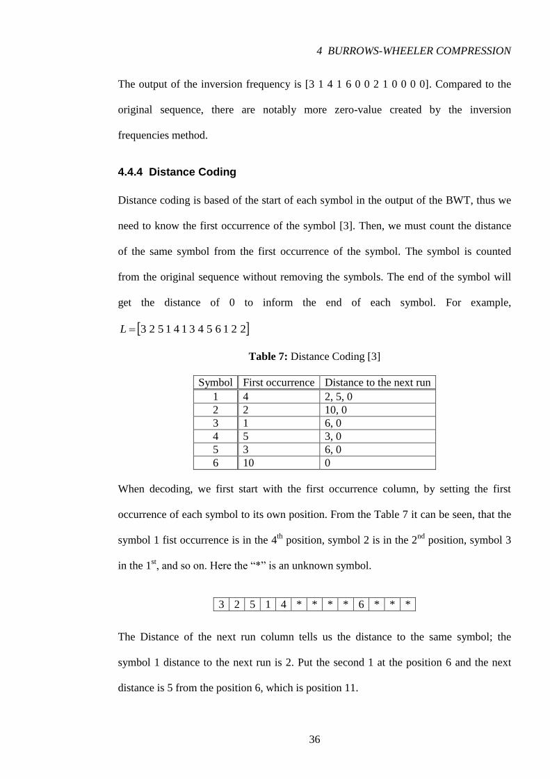
4.4.4 Distance Coding

Distance coding is based of the start of each symbol in the output of the BWT, thus we

need to know the first occurrence of the symbol [3]. Then, we must count the distance

of the same symbol from the first occurrence of the symbol. The symbol is counted

from the original sequence without removing the symbols. The end of the symbol will

get the distance of 0 to inform the end of each symbol. For example,

2216543141523L

Table 7: Distance Coding [3]

Symbol First occurrence Distance to the next run

1 4 2, 5, 0

2 2 10, 0

3 1 6, 0

4 5 3, 0

5 3 6, 0

6 10 0

When decoding, we first start with the first occurrence column, by setting the first

occurrence of each symbol to its own position. From the Table 7 it can be seen, that the

symbol 1 fist occurrence is in the 4th

position, symbol 2 is in the 2nd

position, symbol 3

in the 1st, and so on. Here the “*” is an unknown symbol.

3 2 5 1 4 * * * * 6 * * *

The Distance of the next run column tells us the distance to the same symbol; the

symbol 1 distance to the next run is 2. Put the second 1 at the position 6 and the next

distance is 5 from the position 6, which is position 11.


37

3 2 5 1 4 1 * * * 6 1 * *

After continuing this with all symbols, the final result of decoder of distance coding

became the following sequence, which is the same as the original sequence

2216543141523L

3 2 5 1 4 1 3 4 5 6 1 2 2

4.4.5 Run–Length Encoding

The run-length encoding (RLE) is a simple compression technique, which can be used

either before or after the BWT to reduce the number of runs in data sequence. RLE is

more efficient when the sequence includes much data that is duplicated. The main idea

of RLE is to count the runs that are repeated in the input data and replace the pixels with

a different number of repetitions. For example, the one-dimensional sequence pixels of

input data 1, 1, 1, 2, 2, 2, 3, 3, 3, 4, 4, 4, 4, 4, 4, the pixel “1” has repeated with 3 times,

and the pixel “2” has 4 repetitions, the values can represented as (1,3), (2,4),… The

sequence can be encoded by pairs of (value, repetition) to the end of the original data.

Input data: 1, 1, 1, 2, 2, 2, 3, 3, 3, 4, 4, 4, 4, 4, 4

Encoder: 1, 3, 2, 4, 3, 3, 4, 6

To decode the run-length, the first symbol of the encoder table is known by the value of

the symbol, the second symbol is the repetition of such a value, which is 3 times that of

the symbol 1.

Decoder: 1, 1, 1, X, X, X, X, X, X, X, X, X, X, X, X


38

While decoding to the end of the value, the output of the decoder will becomes exactly

the same as the input data.

Output data: 1, 1, 1, 2, 2, 2, 3, 3, 3, 4, 4, 4, 4, 4, 4

RLE encoding will compress the pixels of the sequence efficiently with the pixels

which contain three or more runs. But if the repetitions of runs are less than 2, there is

no reducing compressed ratio of the sequence [17], [6].

Input data: 1, 1, 2, 3, 3, 4

Encoder: 1, 2, 2, 1, 3, 2, 4, 1

5 EXPERIMENTAL RESULTS

39

Chapter 5: Experimental results

This chapter shows the image compression experimental result of different methods,

and comparisons of images are given for several methods. The results are tabled and

also shown some of the reconstructed images recovered from the original image. The

results are presented for three different image compression techniques, which are

discrete cosine transform, discrete wavelet transform and predictive coding. Included

are methods such as move-to-front, run-length encoding, as well as the Burrows-

Wheeler transform, which has been discussed in previous chapters of the thesis. Also

shown are the results of the effect of different scanning paths; zig-zag, Hilbert, raster

and snake. The image comparisons also have been done for various block sizes.

Huffman coding is the entropy encoding which is used to compress the image data.

Comparisons between the Burrows-Wheeler transform methods and the JPEG standard

is also considered.

5.1 Experimental Data

There are seven test images, which are used for test data – GoldHill, Bridge, Boat,

Barb, Birds, Airplane and Lena.


40

5.2 Explaining Given Methods

There are some abbreviations of different methods shown in this subsection. Here are

some abbreviations along with an explanation of what they stand for:

a) JPEG: JPEG (Joint Photographic Experts Group) standard (Section 3.2)

b) BM: Burrows-Wheeler transform and move-to-front (Section 4.4.2)

c) BR: Burrows-Wheeler transform and run-length encoding (Section 4.4.5)

d) BMR: Burrows-Wheeler transform, move-to-front and run-length encoding

e) Zig-Zag: Zig-zag scanning path (Section 4.4.1.1)

f) Hilbert: Hilbert scanning path (Section 4.4.1.2)

g) Raster: Horizontal raster scanning path scans from the left to right and from

top to bottom (Section 4.4.1.3)

h) Snake: Horizontal snake scanning path starts from the left top corner (Section

4.4.1.3)

i) DWT: Only discrete wavelet transform is used without BWT is applied

(Section 3.3)

j) Predictive: Only predictive coding is used without BWT is applied (Section

3.4)

5.3 Experimental Result using Discrete Cosine Transform

5.3.1 Comparison with Different Methods

This subsection contains an evaluation of the results by applying the discrete cosine

transform. Variations of the Burrows-Wheeler transform are compared to the JPEG

standard. The JPEG standard applies the DCT as a basic technique using the block size

of 8x8. The DCT coefficients are scanned in zig-zag order, and coefficients are


41

encoding with RLE. These techniques are also applied in BM, BR and BMR to give

better comparison for the simulation results.

Table 8 shows that the JPEG standard gives the compression ratio (see Eq. 2.3) of 28:1

on average, while Burrows-Wheeler transform with run length encoding gives a

compression ratio of 30:1. However, the move-to-front method gives over 29:1 on

average. This suggests that, applying the BWT will yield a better result compared to the

original JPEG standard.

Table 8: Comparison of JPEG with BM, BR and BMR

Method GoldHill Bridge Boat Barb Birds Airplane Average

JPEG 24.45 26.34 23.54 31.03 36.90 29.25 28.58

BM 29.68 26.68 22.68 25.68 37.57 31.87 29.05

BR 29.07 26.74 26.19 28.78 34.91 34.05 29.96

BMR 27.39 24.08 20.94 23.40 34.27 31.50 26.92

5.3.2 Effect of Scanning Paths

To evaluate the effect of the different scanning paths used in the study method, we

applied the block size 3232 of the DCT, Burrows-Wheeler transform and run-length

encoding to see the results of each scanning method. Zig-zag, Hilbert, horizontal raster

and horizontal snake scanning methods are performed.

The order of encoding is

- DCT Scanning path BWT RLE

The Table 9 shows that applying the zig-zag scanning path achieved the best

compression ratio which is nearly 30:1, while the Hilbert curve is worst, giving a

compression ratio only on average 29:1.


42

Table 9: Comparing scanning paths

Scan GoldHill Brigde Boat Barb Birds Airplane Average

Zig-Zag 24.52 28.34 25.12 30.91 35.30 33.16 29.56

Hilbert 25.84 23.07 23.07 31.75 33.71 29.89 28.80

Raster 22.08 28.53 24.60 30.79 35.15 34.71 29.31

Snake 22.94 28.94 24.37 30.91 35.30 31.87 29.05

Most of higher frequency coefficients are converted into zeros after the forward discrete

cosine transformation, which are in the right-bottom corner. The zig-zag is suitable for

this situation to scans the sequence of zeros at the end, achieving higher entropy and

run-length coding efficiency.

The difference in results of Table 8 and Table 9 is due to block size of process. In zig-

zag scanning path is applied 3232 , while in BR method the block size is only 88 .

5.3.3 Effect of Block Sizes

In the DCT, the image data is split into smaller block to pre-process the data. Generally,

DCT is broken into 88 blocks of pixels. However, in our application, we also tried

various block sizes. For comparing different block sizes in DCT, we apply six different

block sizes: 22 , 44 , 88 , 1616 , 3232 and 6464 . The DCT coefficients of

the block are scanned using the zig-zag scan and JPEG standard quantization table (see

section 3.3.1).

The order of encoding is following:

- DCT (block size) Zig-Zag BWT RLE


43

Table 10: Comparing block sizes

Block size GoldHill Brigde Boat Barb Birds Airplane Average

22 26.42 26.14 27.38 29.46 32.85 30.71 28.82

44 27.36 24.89 28.00 29.88 34.72 32.64 29.58

88 29.07 26.74 26.19 28.78 34.91 34.05 29.96

1616 21.48 22.92 25.28 20.68 41.79 46.54 29.77

3232 24.52 28.34 25.12 30.91 35.30 33.16 29.56

6464 36.56 25.60 19.68 36.56 25.60 19.68 27.28

From the result shown in the Table 10, it is appear that the block size of 88 gives on

average the best compression ratio, and the next best compression ratio is given by the

block size of 1616 . The worst is the block size of 6464 . Also the block size of

22 and 44 give comparative result in this application. The conclusion of this

subsection is that the small block size gives better result. However the smallest block

size that could be used is 8x8.

The Figure 17 shows the compression ratio for each block size.

Figure 17: DCT with different block size

The Lena image with six different block size of DCT is shown in Figure 18. As can be

observed, the reconstructed image with block size of 88 and 1616 give it visually

almost the same image. But with the block size of 22 and 6464 give a poor

reconstructed image because of the lower compression ratio shown in Table 10.


44

Figure 18: Lena with different blocks size of DCT


45

5.4 Effect of Different Threshold in DWT

In this part, we evaluate the results of different thresholds while using the discrete

wavelet transform for lossy compression. There are three tested methods with three

kinds of thresholds: 10, 30 and 50. In this application we have used Scale 1

decomposition and Scale 2 decomposition for the DWT. The block size of 6464 is

performed.

The orders of encodings are

a) DWT Threshold

b) DWT Threshold BWT MTF

c) DWT Threshold BWT RLE

Table 11a: Scale 1 decomposition with different threshold

Scale 1 Threshold-10 Threshold-30 Threshold-50

Image DWT BM BR DWT BM BR DWT BM BR

GoldHill 23.18 19.97 20.18 28.59 21.52 20.72 32.86 22.53 23.22

Bridge 16.63 14.79 14.88 18.83 14.80 15.55 21.67 15.96 16.45

Boat 18.77 16.64 17.48 22.72 17.02 17.85 27.41 18.68 19.01

Barb 17.74 15.63 15.16 20.04 15.56 16.11 22.70 17.23 17.2

Birds 20.44 17.84 18.33 24.95 18.91 19.05 27.53 20.22 19.63

Airplane 16.79 15.91 14.96 18.77 16.79 16.04 21.96 17.27 16.54

Average 18.52 16.80 16.78 22.32 17.43 17.63 25.68 18.64 18.67

As can be seen from the result in Table 11a, in Scale 1 decomposition, applying the

DWT without any use of Burrows-Wheeler transform will achieve the highest

compression ratio. Obviously, the greater threshold gives the higher compression ratio

compared to the smaller threshold. Here the threshold-50 gives a compression ratio of

almost 26:1, when threshold-10 gives only 18:1. When comparing move-to-front and

run-length-encoding with each other, in threshold-10 move-to-front is slightly better,

but when the threshold is higher, run-length-encoding gives better results.


46

Table 11b: Scale 2 decomposition with different threshold

Scale 2 Threshold-10 Threshold-30 Threshold-50

Image DWT BM BR DWT BM BR DWT BM BR

GoldHill 36.81 25.96 31.02 54.24 30.91 32.83 74.64 37.06 34.78

Bridge 18.27 17.73 16.12 20.67 19.24 17.56 25.06 21.32 18.23

Boat 20.24 18.89 18.24 25.16 20.76 19.72 30.36 30.32 21.21

Barb 20.51 18.63 18.00 25.26 20.24 19.92 30.36 22.40 19.83

Birds 18.33 17.95 16.62 22.22 17.90 17.86 25.28 20.08 18.49

Airplane 22.72 20.90 19.90 26.50 22.42 21.74 33.50 24.14 22.39

Average 22.81 20.00 19.98 29.00 21.91 21.60 36.53 24.94 22.48

The results of Table 11b show that Scale 2 will give a much higher compression ratio

compared to Scale 1 decomposition. Also, independent of the threshold, the move-to-

front method yields a better ratio than the run-length encoding.

5.5 Experimental Result using Predictive Coding

This part of the thesis pre-processes the image data, and then compares it with different

variants of the Burrow-Wheeler-transform, such as move-to-front, run-length-encoding

and also a combination of these two methods. The zig-zag scanning order is applies in

this technique after predictive coding.

By only using predictive coding without including any BWT methods, the compression

ratio will be highest. The next best ratio is to apply the BWT and RLE. When applying

the BWT, MTF and RLE together, the result is the lowest ratio.

Table 12: Predictive coding and different methods of BWT


Predictive 30.00 22.94 25.28 18.32 25.28 20.68 23.74

BM 14.60 13.04 14.296 10.07 12.92 11.40 12.72

BR 23.33 19.08 19.68 14.86 19.83 17.13 18.98

BMR 13.25 11.81 12.85 9.072 11.73 10.35 11.51


47

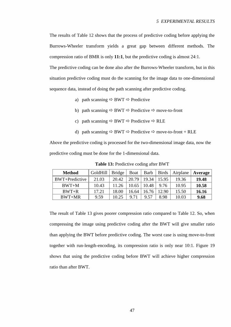
The results of Table 12 shows that the process of predictive coding before applying the

Burrows-Wheeler transform yields a great gap between different methods. The

compression ratio of BMR is only 11:1, but the predictive coding is almost 24:1.

The predictive coding can be done also after the Burrows-Wheeler transform, but in this

situation predictive coding must do the scanning for the image data to one-dimensional

sequence data, instead of doing the path scanning after predictive coding.

a) path scanning BWT Predictive

b) path scanning BWT Predictive move-to-front

c) path scanning BWT Predictive RLE

d) path scanning BWT Predictive move-to-front + RLE

Above the predictive coding is processed for the two-dimensional image data, now the

predictive coding must be done for the 1-dimensional data.

Table 13: Predictive coding after BWT


BWT+Predictive 21.03 20.42 20.79 19.34 15.95 19.36 19.48

BWT+M 10.43 11.26 10.65 10.48 9.76 10.95 10.58

BWT+R 17.21 18.00 16.64 16.76 12.90 15.50 16.16

BWT+MR 9.59 10.25 9.71 9.57 8.98 10.03 9.68

The result of Table 13 gives poorer compression ratio compared to Table 12. So, when

compressing the image using predictive coding after the BWT will give smaller ratio

than applying the BWT before predictive coding. The worst case is using move-to-front

together with run-length-encoding, its compression ratio is only near 10:1. Figure 19

shows that using the predictive coding before BWT will achieve higher compression

ratio than after BWT.


48

Figure 19: Predictive coding before and after BWT

As can be seen at Figure 19, the use of the Burrows-Wheeler transfrom before

predictive (BWT+P) will achieve quite good compression ratio compared to the use of

the Burrows-Wheeler transform before run-length encoding (BWT+R). The applying of

the Burrows-Wheeler transform gave worst compression ratio.

5.5.1 Effect of Scanning Paths on Predictive Coding

To compare different scanning path, here we also apply the same scanning paths as

before: zig-zag, Hilbert, Raster and Snake.

The phase of using predictive coding for the scanning path is the following:

- Predictive Coding Scanning path BWT RLE

There are four path scanning methods being applied, it is noticeable that the raster and

the snake scanning did not give any significant advantages of compression performance.

As Table 14 shows, every scanning method gave almost the same compression ratio

after applying the BWT and RLE. However the zig-zag scanning path gives the best

overall result compared to the others.


49

Table 14: Predictive coding and different methods of BWT

Scan GoldHill Brigde Boat Barb Birds Airplane Average

Zig-Zag 23.33 19.08 19.68 14.86 19.83 17.13 18.98

Hilbert 22.13 19.00 19.22 14.88 18.32 16.12 18.28

Raster 22.81 19.544 19.36 14.54 17.68 16.31 18.37

Snake 23.60 18.96 18.16 14.54 19.00 15.90 18.36

6 CONCLUSIONS

50

Chapter 6: Conclusions

In this thesis, the use of the Burrows-Wheeler transform in image compression was

studied. A few discrete transformations, as well as predictive coding were considered.

The difference of the quantization block sizes are presented and have been shown the

results for the effect of the various block size of quantization table. Several

linearization techniques were introduced to convert the 2-dimensional image to 1-

dimensional linear data sequence. Also, variants of the Burrows-Wheeler transform

methods have been considered.

The experimental results show that application the Burrows-Wheeler transformation

gives a slightly improved performance on average compared to the JPEG standard.

Also a combination of BWT with move-to-front and run-length encoding yield even

better results when compared to JPEG standard. For linearizing the image a into linear

pixel sequence by zig-zag scanning path after pre-processing with the discrete cosine

transform gives the best result compared to the other scanning methods such as the

raster, the snake or the Hilbert scanning path. Furthermore, the raster scan and the snake

scan are competitive methods that were discovered while studying methods for

linearizing the pixels sequence. As results show, the block size of 88 applying in

6 CONCLUSIONS

51

DCT will achieve a better result in the instance of using 22 , 44 , 1616 , 3232

or 6464 block sizes. But the neighboring block size of 88 are gave quite good

compression ratio compared to, for example, the block size of 22 and 6464 . The

Figure 18 showed the discrete cosine transform with different block sizes, visually the

block size of 88 gave the best result for the reconstructed image.

The effect of using a different threshold will play an important role while processing a

discrete wavelet transform. The experimental result shows that when tested the DWT

with a higher threshold, the reconstructed image compression is better than in the case

of a smaller threshold. This is noticeable from the pre-processing image, because the

higher threshold will yield much more zeros at details coefficients of DWT. Scale 2

decomposition of DWT yields also a better compression ratio result, but on the other

hand, the reconstructed image is poorer than by applying only scale 1 decomposition.

For predictive coding, the uses of the Burrows-Wheeler transform and other variants of

the BWT did not yield any better average results than applying only the predictive

coding for image compression. The use of predictive coding after the Burrows-Wheeler

transform as well as the move-to-front and the RLE was also tested. The result did not

gave any better compression ratio compared to the predictive used before the Burrows-

Wheeler transform. The use of a zig-zag scanning path gives also the best result in

predictive coding as well as in DCT.

Generally, the use of Burrows-Wheeler Transform is suitable for image compression as

well as others standard compression methods. When using discrete cosine transform

with zig-zag scanning path and run-length coding, the result of compression ratio will

even better than JPEG standard. On the other hand, one additional method causes an

6 CONCLUSIONS

52

extra execution time in the processors, because of the slowness in processing steps of

BWT, which is a one of drawbacks when using this technique.

In the future the study will concentrate on different improvement algorithms of BWT to

minimize execution time and the study of the compression in speech and video data

using Burrows-Wheeler Transform.

REFERENCES

53

References

[1] Yun Q. Shi and Huifang Sun, Image and Video Compression for Multimedia

Engineering, 2nd

edition, CRC Press, 2008.

[2] Khlid Sayood, Introduction to Data Compression, 2nd

edition, Morgan Kaufmann

Publishers, CA, 2000.

[3] Donald Adjerob, Timothy Bell and Amar Mukherjee, The Burrows-Wheeler

Transform: Data Compression, Suffix Arrays, and Pattern matching, Springer, New

York, 2008.

[4] R. C. Gonzalez and R. E. Woods, Digital Image Processing, 2nd

edition, Prentice

Hall, New Jersey, 2002.

[5] R. C. Gonzalez, R. E. Woods, S. L. Eddins, Digital Image Processing Using Matlab,

Prentice Hall, New Jersey, 2004.

[6] Nandakishore R. Jalumuri, A Study of Scanning Paths for BWT Based Image

Compression, Master’s thesis, Morgantown, West Virginia 2004.

[7] M. Burrows and D.J. Wheeler, A Block-sorting Lossless Data Compression

Algorithm, Research Report 124, System Research Center, Digital System Research

Center, Palo Alto, CA, 1994.

REFERENCES

54

[8] Ziya Arnavut and Spyros S. Megluveras, Block Sorting and Compression. Data

Compression Conference 1997: 181-190.

[9] Sanjiv K. Bhatia, Visual Data Processing, Lecture note, May 2006.

[10] Paymen Zehtab Fard, Still Image Compression, Lecture note, 1996.

[11] Ingela Nyström, Image Coding and Compression, Centre for Image Analysis,

Uppsala Universitet, November 2007.

[12] Kang-Hua Hsu, introduction to wavelet transform and image compression,

Graduate Institute of Communication Engineering, National Taiwan University, Taipei,

Taiwan.

[13] Yao Wang, Wavelet Transform and JPEG2000, Polytechnic University, Brooklyn,

NY 11201, USA

[14] Sharon Shen, Discrete Wavelet Transform (DWT), Lecture note, University of

Maryland, Baltimore County, 2006

[15] Kharate, Patil and Bhale, Selection of Mother Wavelet For Image Compression on

Basis of Nature of Image, Journal of Multimedia, Vol. 2, No. 6, November 2007.

[16] Ayadi, Syiam and Gamgoum, Comparative Study of Lossy Image Compression

Techniques, IJCIS, Vol.6, No.1, January 2006.

[17] Arturo San Emeterio Campos, Run Length Encoding, Arturo San Emeterio

Campos, Barcelona 1999.

[18] Pizurica and Philips, Digital Image Processing, Ghent University, Lecture notes in

Computer science, January 2007.

[19] Subramanya and Youssef, Performance Evaluation of Lossy DPCM Coding of

images Using Different Predictors and Quantizers, ISCA CAINE98 Conference, Las

Vegas, Nevada, November 1998.

http://www.cs.umsl.edu/~sanjiv/classes/cs5420/lectures/compress.pdf

http://www.seas.gwu.edu/~ayoussef/papers/LossyDPCM-ISCA98

http://www.seas.gwu.edu/~ayoussef/papers/LossyDPCM-ISCA98

REFERENCES

55

[20] S. P. Nanavati and P. K. Panigrahi, Wavelet: Application to Image Compression-II,

Springer India, in co-publication with Indian Academy of Sciences, Volume 10, Number

3 / March, 2005

[21] Mariusz Jankowski, Digital Image Processing, Mathematica Second Edition

Published by Wolfram research, 2007

[22] A Mathematical Theory of Communication, C. E. Shannon, The Bell System

Technical Journal, Vol. 27. pp. 379-423, 623-656, July, October, 1948

[23] Ping-Sing Tsai and Tinku Acharya, Image Up-Sampling Using Discrete Wavelet

Transform, JCIS-2006 Proceedings, October 2006

[24] Oge Marques, Image Compressiong and Coding, Department of Computer Science

and Engineering, Florida Atlantic University, Boca Raton, FL, USA

[25] Myllyoja Jani, Burrows-Wheeler-pakausmenetelmä ja sen variaatiot, Master’s

Thesis, Turku University , Summer 2003

[26] Mauro Barmi, Document and image compression, CRC Press, USA, 2006

http://www.springerlink.com/content/p716p41183h4/?p=c24f0dd067bd4d07be0f5cbcff327ad9&pi=0

http://www.springerlink.com/content/p716p41183h4/?p=c24f0dd067bd4d07be0f5cbcff327ad9&pi=0

http://www.wolfram.com/products/applications/digitalimage/quicktour/representat%20ion.html

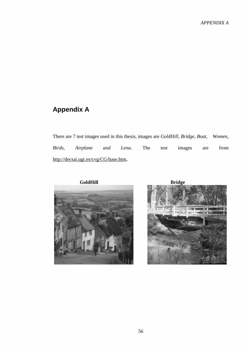
APPENDIX A

56

Appendix A

There are 7 test images used in this thesis, images are GoldHill, Bridge, Boat, Women,

Birds, Airplane and Lena. The test images are from

http://decsai.ugr.es/cvg/CG/base.htm.

GoldHill Bridge

http://decsai.ugr.es/cvg/CG/base.htm

APPENDIX A

57

Boat Barb

Birds Airplane

Lena

image compression using burrows-wheeler transformlib.tkk.fi/dipl/2009/urn100116.pdf · image...

Documents