iise user manual - vrtech – tecnologias...
TRANSCRIPT

iiSE
Industrial Integrated
Simulation Environment
User Guide
www.vrtech.com.br
September 18, 2015

Contents
1 Introduction 1
1.1 Introduction to iiSE . . . . . . . . . . . . . . . . 2
1.2 Technology . . . . . . . . . . . . . . . . . . . . . 2
1.2.1 Thermodynamic Packages . . . . . . . . . 3
1.2.2 Equation-oriented approach . . . . . . . . 3
1.2.3 Developed using Java© . . . . . . . . . . 4
1.3 Installation . . . . . . . . . . . . . . . . . . . . . 4
1.4 Compatibility . . . . . . . . . . . . . . . . . . . . 5
2 Getting Started 6
2.1 Starting iiSE . . . . . . . . . . . . . . . . . . . . 7
2.2 Creating a new Project . . . . . . . . . . . . . . 8
2.3 Process �owsheet diagram . . . . . . . . . . . . . 11
2.3.1 Menu Bar . . . . . . . . . . . . . . . . . 12
2.3.2 Button bar . . . . . . . . . . . . . . . . . 13
2.3.3 Library Palette . . . . . . . . . . . . . . . 13
2.3.4 Center Page . . . . . . . . . . . . . . . . 14
2.3.5 Variables tab . . . . . . . . . . . . . . . . 14
2.3.6 Satellite view . . . . . . . . . . . . . . . . 15
2.3.7 Message bar . . . . . . . . . . . . . . . . 15
2.3.8 Status Bar . . . . . . . . . . . . . . . . . 16
2.3.9 Progress Bar . . . . . . . . . . . . . . . . 17
2.4 Hot keys . . . . . . . . . . . . . . . . . . . . . . 19

3 Creating Simulation Diagrams 20
3.1 Degrees of Freedom . . . . . . . . . . . . . . . . 21
3.2 Equation Oriented solution . . . . . . . . . . . . 21
3.3 Equipments Overview . . . . . . . . . . . . . . . 22
3.4 Connecting devices . . . . . . . . . . . . . . . . . 23
3.5 Specifying variables . . . . . . . . . . . . . . . . 24
3.6 Matching the degrees of freedom . . . . . . . . . 25
3.7 Observability and Redundancy Report . . . . . . . 30
3.8 Solving a simulation . . . . . . . . . . . . . . . . 39
3.9 Visualizing the Results . . . . . . . . . . . . . . . 39
4 Water Steam Library 43
4.1 Introduction . . . . . . . . . . . . . . . . . . . . 44
4.2 Streams . . . . . . . . . . . . . . . . . . . . . . 45
4.2.1 Material stream for water and steam . . . 45
4.2.2 Energy Stream . . . . . . . . . . . . . . . 46
4.3 Equipment Models . . . . . . . . . . . . . . . . . 47
4.3.1 Source Saturated . . . . . . . . . . . . 47
4.3.2 Source . . . . . . . . . . . . . . . . . . . 48
4.3.3 Sink . . . . . . . . . . . . . . . . . . . . 49
4.3.4 Source Sugar . . . . . . . . . . . . . . . 49
4.3.5 Energy Source . . . . . . . . . . . . . . 50
4.3.6 Energy Source Gross HV . . . . . . . . 51
4.3.7 Turbine . . . . . . . . . . . . . . . . . . 52
4.3.8 Turbine Bleeding . . . . . . . . . . . . 52
4.3.9 Boiler . . . . . . . . . . . . . . . . . . . 53
4.3.10 Evaporator . . . . . . . . . . . . . . . . 54
4.3.11 Boiler Reheat . . . . . . . . . . . . . . 55
4.3.12 Pump . . . . . . . . . . . . . . . . . . . 56
4.3.13 Condenser . . . . . . . . . . . . . . . . 57
4.3.14 Heater . . . . . . . . . . . . . . . . . . . 58

4.3.15 Heat Exchanger . . . . . . . . . . . . . 59
4.3.16 Mixer . . . . . . . . . . . . . . . . . . . 60
4.3.17 Splitter . . . . . . . . . . . . . . . . . . 61
4.3.18 Recycle . . . . . . . . . . . . . . . . . . 62
5 Process Engineering Library 63
5.1 Introduction . . . . . . . . . . . . . . . . . . . . 64
5.2 Thermodynamics . . . . . . . . . . . . . . . . . . 65
5.2.1 Cubic equations of state . . . . . . . . . . 67
5.2.2 Activity/Gibbs excess models . . . . . . . 69
5.2.3 FA-ME-W Package . . . . . . . . . . . . . 70
5.2.4 Petroleum modeling . . . . . . . . . . . . 73
5.3 Streams . . . . . . . . . . . . . . . . . . . . . . 75
5.3.1 Material stream . . . . . . . . . . . . . . 75
5.3.2 Energy Stream . . . . . . . . . . . . . . . 76
5.4 Equipment Models . . . . . . . . . . . . . . . . . 77
5.4.1 Source . . . . . . . . . . . . . . . . . . . 77
5.4.2 Sink . . . . . . . . . . . . . . . . . . . . 77
5.4.3 Mixer . . . . . . . . . . . . . . . . . . . 78
5.4.4 Mixer3 . . . . . . . . . . . . . . . . . . 79
5.4.5 Splitter . . . . . . . . . . . . . . . . . . 80
5.4.6 Energy Source . . . . . . . . . . . . . . 80
5.4.7 Energy Source Gross HV . . . . . . . . 81
5.4.8 Energy Splitter . . . . . . . . . . . . . 82
5.4.9 Flash . . . . . . . . . . . . . . . . . . . 82
5.4.10 FlashPH . . . . . . . . . . . . . . . . . 84
5.4.11 Flash-VLL . . . . . . . . . . . . . . . . 85
5.4.12 Column . . . . . . . . . . . . . . . . . . 86
5.4.13 Separator . . . . . . . . . . . . . . . . . 87
5.4.14 Compressor . . . . . . . . . . . . . . . . 88
5.4.15 Turbine . . . . . . . . . . . . . . . . . . 89

5.4.16 Pump . . . . . . . . . . . . . . . . . . . 90
5.4.17 Equilibrium Reactor . . . . . . . . . . . 91
5.4.18 Gibbs Reactor . . . . . . . . . . . . . . 92
5.4.19 Stoichiometric Reactor . . . . . . . . . 93
5.4.20 Heat Exchanger . . . . . . . . . . . . . 94
5.4.21 Heater . . . . . . . . . . . . . . . . . . . 95
5.4.22 Cooler . . . . . . . . . . . . . . . . . . . 96
5.4.23 Recycle . . . . . . . . . . . . . . . . . . 97
5.4.24 Valve . . . . . . . . . . . . . . . . . . . 98
6 Interfaces with other software 100
6.1 Variable links . . . . . . . . . . . . . . . . . . . . 101
6.2 Microsoft Excel©Add-in . . . . . . . . . . . . . . 101
6.3 Java, Scilab, and Matlab interfaces . . . . . . . . 105
6.3.1 Preparing the CLASSPATH . . . . . . . . 105
6.3.2 Using the iiSE simulation engine . . . . . . 106
6.3.3 Thermodynamics server . . . . . . . . . . 107
6.4 Python gateway . . . . . . . . . . . . . . . . . . 111
6.4.1 Simulation engine . . . . . . . . . . . . . 111
6.4.2 Thermodynamics server . . . . . . . . . . 112
6.5 EMSO . . . . . . . . . . . . . . . . . . . . . . . 114
6.5.1 Plugin con�guration . . . . . . . . . . . . 114
6.5.2 Exporting iiSE simulations to EMSO . . . 115
References 116

Copyright
The Copyright of this software, guide, examples and otherdocuments are property of VRTech Tecnologias Industriais Ltdaand are sold or distributed according to the license that hasuse restrictions.
The copy, distribution, reproduction of this software andassociated documents as a whole or in parts under any way(electronic, recording, photocopy, internet distribution andothers) is prohibited without the written permission of VRTechTecnologias Industriais Ltda.
(C) 2006-2012 VRTech Tecnologias Industriais Ltda.
All rights reserved.
iiSE is a VRTech Tecnologias Industriais Ltda() property.All other brand and product names are trademarks or registeredtrademarks of their respective companies.All rights reserved.

Symbols e Conventions
In this document, some symbols and conventions are adopted:
Commands or �les: commands and �le names inserted in thetext are emphasized as: command and file.
Note: Sometimes, important information is given as a note, e.g.:iiSE is an equation�oriented simulator.
Warning: To highlight possible problems or good practices inprocess simulation, e.g.: It is important to choose the appropriatethermodynamic model.
Tip: Helpful hint for the user, e.g.: For mixtures containing polarsubstances, choose UMR or UGMR mixing rule.
Linux: Speci�c note for POSIX platform (Linux and Unix).
Windows: Speci�c note for Win32 platform (Windows 95 andderivatives, Windows NT 4 and derivatives).
Under Development: Noti�es a topic under construction.

Suport, Contact and Updates
For iiSE suport, contact VRTech:
� On the internet www.vrtech.com.br
� By e-mail [email protected]
iiSE is under continuous developmment, so please feel free to contact us with suggestions,bug reports or any other issues.

1 Introduction
In this chapter iiSE process simulator is brie�y presented with its main structural features.Simple installation instructions are depicted at the end of this chapter.
Contents
1.1 Introduction to iiSE . . . . . . . . . . . . . . . . . . . . . . . . . . 2
1.2 Technology . . . . . . . . . . . . . . . . . . . . . . . . . . . . . . . 2
1.3 Installation . . . . . . . . . . . . . . . . . . . . . . . . . . . . . . . 4
1.4 Compatibility . . . . . . . . . . . . . . . . . . . . . . . . . . . . . . 5

2 1 Introduction
1.1 Introduction to iiSE
iiSE (read easy) is a steady state process simulator based on theequation-oriented technology. Some of the most important unitoperations present in chemical and petrochemical industries aswell as energy generation and co-generation processes are avail-able in the iiSE model libraries.
iiSE has a physical and thermodynamic data bank with more than1200 compounds and speci�c data for water and steam processes(IAPWS [14]). The most recent thermodynamic models (equa-tions of state, mixing rules, activity models) are implemented toensure a good representation of pure substance and mixture be-havior.
iiSE (read easy) is an acronym for Industrial Integrated SimulationEnvironment. Its main goal is to consolidate a process simulatorwith friendly user interface, capable of simulate complex diagramswith just few clicks in an easy and intuitive way.
iiSE is continuously under development. Any king of feed-back istruly appreciated regarding the following aspects:
� results report;
� graphic user interface;
� communication with other softwares;
� new equipment models;
� new thermodynamic models;
� documentation improvements;
always focusing the �nal user needs.
1.2 Technology
iiSE development is based on modern technologies:
� the most recent thermodynamic models for mixture prop-erties evaluation, more details in section 5.2;
� equation-oriented approach with enhanced convergence pro-cedures;
� written in Java language with solvers and optimizers writtenin C, C++ and FORTRAN.

1.2 Technology 3
1.2.1 Thermodynamic Packages
Regarding water and steam processes, iiSE counts with an imple-mentation of the IAPWS formulation, precise for industrial andscienti�c use [14]. The formulation is valid in the entire stable�uid region from the melting curve to 1273 K at pressures to1000 MPa. It extrapolates in a physically reasonable way outsidethis region. For more details, please check chapter 4.
For process engineering processes, iiSE implements modern pre-dictive thermodynamic models for mixture calculations. The mostrecently developed mixing rules are available (PSRK, UMR, UGMR,SCMR) coupling the classical cubic equations of state with ac-tivity coe�cient models (UNIFAC (Do), UNIFAC (PSRK), etc.).This enables the representation of highly asymmetric mixturesand/or mixture behavior in high conditions of temperature andpressure without the need of empirical corrections. For more de-tails please check chapter 5.
1.2.2 Equation-oriented approach
Most of the commercial simulators available today are based onthe old sequential-modular technology, which requires an indi-vidual calculation engine for each equipment in the �owsheet.Further, another convergence mechanism is needed for diagramswith recycle streams. This thechnology impose several limitationsto the user. For instance, the possible variable speci�cations arecompletely dependent on the implementation available.
iiSE software, on the other hand, implements the equation-orientedconcept, also known as the simultaneous solution technology. Asa consequence, the user speci�cations are not limited to eachpiece of equipment and hence a more �exible set of speci�ca-tions is possible as long as the global degree of freedom is re-spected. In this way, a broader view of the entire �owsheet ispossible and processes with internal recycles are directly treated.Equation-oriented simulators are also taken as better for processoptimization.
Regarding processes with recycle streams, the equation-orientedmethod has some advantages. In the example of Figure 1.1 aprocess of methanol and ketone separation is shown. This mixturehas an azeotrope and needs two distillation columns for completeseparation. The columns operate in di�erent pressures for theazeotrope separation (pressure swing system). The top product ofone column is recycled to the �rst one. This process is simulatedusing iiSE without any problem or special care.

4 1 Introduction
Figure 1.1: Example ofprocess with recycle.
1.2.3 Developed using Java©
Java© is an object oriented language that brings several advan-tages for developers and �nal users.
Java© is maintained by Sun Microsystems©, which providesupdates and new features are implemented by experienced pro-fessional that guarantees highly e�cient and bug free code. Javahas a huge development community and also many software engi-neering tools which makes the software development and deployfast and e�cient. For the �nal user it means an inexpensive, fast,robust and user friendly software with advanced features.
Java© software can be used in di�erent platforms, such as Win-dows, Linux and the web.
Other commercial process simulators are developed in old pro-gramming languages such as FORTRAN or C, making the codemaintenance and deployment di�cult. This ends up forcing tosupport a single platform.
1.3 Installation
The iiSE demonstration version can be installed by simply unzip-ping the downloaded package to an appropriate folder.
The full version comes blunded in a setup wizard, in that casejust follow the on screen instructions.
1.4 Compatibility 5
Windows: In order to start the iiSE program simply double clickon the iise.exe �le.
Linux: iiSE can be launched either by double clicking in theexecutable �le named iiSE or iise.desktop or from theterminal by running the iise.desktop.sh script.
1.4 Compatibility
iiSE is compatible with all Windows versions supported by Mi-crosoft, from Windows XP to Vista and Seven and is also com-patible with most recent Linux distributions.
Please let us know if any environment incompatibility is found.

2 Getting Started
In this Chapter, the main features of iiSE user's interface and its basic functionalities aredescribed.
Contents
2.1 Starting iiSE . . . . . . . . . . . . . . . . . . . . . . . . . . . . . . 7
2.2 Creating a new Project . . . . . . . . . . . . . . . . . . . . . . . . 8
2.3 Process �owsheet diagram . . . . . . . . . . . . . . . . . . . . . . 11
2.4 Hot keys . . . . . . . . . . . . . . . . . . . . . . . . . . . . . . . . 19

2.1 Starting iiSE 7
2.1 Starting iiSE
Once you start iiSE, an initial screen as the one illustrated inFigure 2.1 appears.
Note: Sometimes, the screen shots presented in this guide maydi�er from those found by the user. This is due to di�erences inuser con�gurations, operational systems and software updates.
Figure 2.1: Initial iiSE screenshot.
In the �rst iiSE window, the following options are available:
� Common Actions: Create a new project, open existingproject, quit simulator.
� Recent Projects: last projects list with its respective dateand time of last change.
� Example Projects: list of simulation cases distributedwith iiSE.
In the list of simulation cases included in iiSE distributions, clas-sic literature problems as well as special simulation cases can befound as multiple phases equilibrium and process mass and heatintegration. The preliminary list of cases is shown in Figure 2.2.
It is worth mentioning that the functionalities found in CommonActions options are also available from File menu on the maintool bar.

8 2 Getting Started
Figure 2.2: List of simulationcases of iiSE distribution.
2.2 Creating a new Project
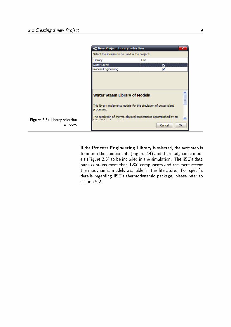
When a New Project option is chosen, a window like the one inFigure 2.3 is opened. In this window the user selects the librariesavailable in iiSE simulator.
The Water Steam library contains speci�c routines to evaluatesteam power cycles, thermodynamic and physical properties ac-cording to IAPWS95. More details about this library of modelscan be found in chapter 4.
The Process Engineering Library holds the main models neededto represent an industrial process: distillation columns, separationdevices, reactors, heat exchangers, pumps compressors, valvesand etc. More details about this library of models can be foundin chapter 5.
Warning: After selecting the libraries to be used, it is not possibleto change the libraries for the project.
2.2 Creating a new Project 9
Figure 2.3: Library selectionwindow.
If the Process Engineering Library is selected, the next step isto inform the components (Figure 2.4) and thermodynamic mod-els (Figure 2.5) to be included in the simulation. The iiSE's databank contains more than 1200 components and the more recentthermodynamic models available in the literature. For speci�cdetails regarding iiSE's thermodynamic package, please refer tosection 5.2.

10 2 Getting Started
Figure 2.4: Addingcomponents to the simulation.
Figure 2.5: Setting thethermodynamic models of the
simulation.

2.3 Process �owsheet diagram 11
Tip: If the Process Engineering Library was selected, thethermodynamic models can be freely changed during the projectconstruction.
2.3 Process �owsheet diagram
After the initial con�gurations (libraries, components and thermo-dynamic models) a blank diagram is presented like in Figure 2.6.
Figure 2.6: Initial blankdiagram.
Around the blank �owsheet area, the following functionalities canbe identi�ed:
1. Menu bar;
2. Button bar;
3. Library Pallet;
4. Center Page;
5. Variable area;
6. Satellite view;
7. Message bar;

12 2 Getting Started
8. Status bar;
9. Progress bar.
2.3.1 Menu Bar
Through the menu bar the user can access the basic actions ofiiSE simulator.
Note: iiSE projects are store in �les with the .ise extension.
The following operations are found in the File menu:
� New Project: Creates a new project like shown in sec-tion 2.2. If an existing project is already opened with un-saved modi�cations, it is asked for the user to save thecurrent project before creating a new one.
� Save: Saves the current project. If a project is been savedfor the �rst time a new window is opened to set the �lename and location.
� Open Project ...: Opens an existing project. If a projectis already opened with unsaved modi�cations, it is asked forthe user to save the current project before opening a newone.
� Save as ...: Saves the existing �le in a di�erent path orname.
� Close Project: Closes the current opened project. If the�le is not saved, iiSE will ask for Save the project. Afterclosing project the simulator goes back to the initial screen(section 2.3).
� Quit: Quit the program. Before closing the simulator, theuser will be asked to save the unsaved modi�cations to avoidloosing the work done.
In View Menu it is possible to adapt the simulator interface,activating/deactivating the following tools:
� Palette;
� Satellite View;
� Variables.
Besides show or hide the di�erent tools, the user can change itsposition in the interface.

2.3 Process �owsheet diagram 13
In Simulation menu the following buttons can be found:
� Run: Runs the simulation �owsheet.
� Report: Shows the results of a simulation for the selectedequipment.
� Cancel: Cancels the simulation.
It is worth mentioning that before running a simulation it is nec-essary to ful�ll the degrees of freedom of the �owsheet with theequipment speci�cations. The Report action needs a completesimulation run to be activated.
Canceling a simulation can be a useful option in cases where thesimulation is taking too much time caused by bad user speci�ca-tions or numerical instabilities.
In the Help Menu, basic information about iiSE software areavailable in the About option.
2.3.2 Button bar
The button bar contains shortcuts to the most common actions
Figure 2.7: Button bar.
1. Create a new project;
2. Save project;
3. Open project;
4. Run simulation.
These functionalities are the same as those presented in the Menubar section.
2.3.3 Library Palette
The Library palette is displayed, by default, to the left of thecentral page Using the Library palette, all pieces of equipment ofthe selected libraries can be accesses by the user to create a newproject.
It is also possible to contract or expand each library clicking onthe right icon of library's name.
For further details about the libraries, see chapter 4 and chapter 5.

14 2 Getting Started
Figure 2.8: Library Palette.
2.3.4 Center Page
The central page is the space where the simulation diagram isbuilt, containing the equipment and streams that connect them.
In order to add new devices to the simulation �owsheet, a singleclick is required on the equipment icon in the library palette. Thedevice will appear in the main diagram as shown in Figure 2.9.The device can be renamed (by clicking twice on the originalname), moved, resized (using the small square in the lower-rightcorner of the selected equipment) the little square in the rightlower corner) and connected to other equipment through its outletconnections.
The user can zoom-in to get a closeup view of the diagram orzoom-out to see more of the page at a reduced size. To do so, itis necessary to right click on a empty diagram area.
2.3.5 Variables tab
In the variables tab the variables of the currently selected equip-ment are shown, as can be seen in Figure 2.10.
Actually, the variables tab comes with more information than thelist of variables:
� Table with model variables, its values and units of measure;

2.3 Process �owsheet diagram 15
Figure 2.9: Center page witha compressor.
� Brief description, lower and upper bounds of each variable;
� Local degree of freedom (Local DF);
� Results status.
In the variable table the user must close the degrees of freedomto run a simulation.
If no equipment was selected, in the variable area the message NoObject Selected is presented. The message Results outdatedmeans that the shown variable values were not updated with thelast modi�cations in the �owsheet. After a simulation run themessage Results Available is shown.
2.3.6 Satellite view
The satellite view consists of a small scale reproduction of thediagram. It is very useful when a big diagram is been built, allow-ing an overview of the entire �owsheet. Also, it o�ers a simpleway to navigate through the diagram, by simply clicking on thedesired location or dragging the frame corresponding to the viewof the central page.
2.3.7 Message bar
The message bar shows the current state diagram simulation. Themessages shown are as follows:

16 2 Getting Started
Figure 2.10: Variables forthe model of a compressor.
When starting a new �owsheet, the following messages can bedisplayed:
� Diagram is Empty. This message appears when a newproject is created or when all equipment of a diagram areremoved.
� Add/remove specs to close the DF. This message ap-pears when a new equipment is added to the diagram andremains until the global degree of freedom is ful�lled. Forfurther details about DF, see section 3.1 and section 3.6.
� Results Outdated, run a simulation. This messageindicates that a simulation can be run in order to updatethe variable values.
� Results available. This message indicated that the sim-ulation was completed successfully and the variable valueswere updated.
2.3.8 Status Bar
The status bar indicates the total degree of freedom of the dia-gram.

2.3 Process �owsheet diagram 17
Figure 2.11: Satellite view ofa �owsheet.
Figure 2.12: Message bar.
2.3.9 Progress Bar
Through the progress bar, the user can visualize the simulationprogress.
The numerical methods of simulation resolution, whenever pos-sible, split the global problem in smaller subproblems, and theprogress bar gives the user an idea of the progress of the resolu-tion of the simulation.
Figure 2.13: Degree offreedom.

18 2 Getting Started
Figure 2.14: Progress bar.

2.4 Hot keys 19
2.4 Hot keys
Some of the most frequent actions may be accomplished usingshortcuts as shown in Table 2.1.
Action Hot keySave current project ctrl + S
Run simulation ctrl + RCancel simulation ctrl + bckspc
Quit iiSE alt + F4
Table 2.1: Hot keys.

3 Creating Simulation Diagrams
In the Chapter that follows, some important concepts are presented: degrees of freedom,equation oriented solution and redundancy. Also, the creation of simulation diagrams isshown along with the tools for result analysis.
Contents
3.1 Degrees of Freedom . . . . . . . . . . . . . . . . . . . . . . . . . . 21
3.2 Equation Oriented solution . . . . . . . . . . . . . . . . . . . . . . 21
3.3 Equipments Overview . . . . . . . . . . . . . . . . . . . . . . . . . 22
3.4 Connecting devices . . . . . . . . . . . . . . . . . . . . . . . . . . 23
3.5 Specifying variables . . . . . . . . . . . . . . . . . . . . . . . . . . 24
3.6 Matching the degrees of freedom . . . . . . . . . . . . . . . . . . 25
3.7 Observability and Redundancy Report . . . . . . . . . . . . . . . . 30
3.8 Solving a simulation . . . . . . . . . . . . . . . . . . . . . . . . . . 39
3.9 Visualizing the Results . . . . . . . . . . . . . . . . . . . . . . . . 39

3.1 Degrees of Freedom 21
It is worth recalling that the iiSE is based on the equation orientedapproach in which the �nal system of equations to be solved ina simulation contains all the equations (and variables) of eachequipment added to the diagram. Once the degrees of freedomof such system are satis�ed, the software proceeds the solution ofthe simulation.
3.1 Degrees of Freedom
The de�nition of degrees of freedom for process simulation isrepresented by the following equation:
DF = Nvars −Neqs −Nspec (3.1)
Where:DF : Degrees of freedomNvars: Number of variablesNeqs: Number of equationsNspecs: Number of speci�cations
In order to match the global DF of a simulation, DF speci�cationsmust be provided by the user. The global degree of freedom of asimulation diagram (Global DF) is shown in the status bar as insubsection 2.3.8.
Each model available in the iiSEModel Library have its own
equations and variables. When anew device is inserted into the
�owsheet, its equations andvariables are added to the global
system of equations and the globalDF is modi�ed.
For each model, the degrees of freedom are also available for theuser and are called as Local DF. As a general recommendation,each model should have its degrees of freedom satis�ed to matchthe global DF, but in some cases, it is possible to over specifyone device and under specify another in order to close the globalDF. More information about model speci�cations can be found inChapters 4 and 5.
3.2 Equation Oriented solution
In iiSE the NLA (non-linear algebraic system of equations) result-ing from the process �owsheet is solved using speci�c methods.The mentioned system is represented by:
F (x) = 0subject toxl ≥ x ≥ xu
, (3.2)
where F (x) is the total set of equations containing each modelequations and the �owsheet speci�cations, x are the variables ofthe systems and xl and xu are, respectively, the lower and uppervariable boundaries.

22 3 Creating Simulation Diagrams
3.3 Equipments Overview
Basically, all devices contain a mathematical model (that is, vari-ables and equations), inlet and outlet streams, which can be mate-rial or energy streams. In the diagram, the inlets are representedby blue squares with a dark spot in the center and outlets arerepresented by blue squares.
Figure 3.1 presents a compressor device with 2 inlets and 1 outlet.
Figure 3.1: Representationof a compressor instance.
Source and sink are special equipments used in almost all dia-grams. They are included into the �owsheet to de�ne generalinlets and outlets of the whole process. These instances haveonly one connection port (inlet or outlet) and variables used todescribe material or energy streams.
While a Source stream contains only one outlet and requires userspeci�cations (one for energy source and three for material source)the Sink stream does not alter the diagram DF and contains onlyone inlet port. In Figure 3.2 a Source stream is connected to aSink stream as an example of ports compatibility.
Figure 3.2: Source and Sinkstream in a illustrative
diagram.

3.4 Connecting devices 23
3.4 Connecting devicesMaterial streams are compatible,and consequently, allowed to be
connected as long as they belongto equipments from the same
model library. Otherwise, energystreams can be freely connected
between libraries in order to allowprocess heat integration studies.
To connect the devices of a simulation diagram, it is just click theleft-click button on the outlet icon of one equipment and drag itto an inlet port of the desired device, as represented in Figure 3.3.A stream is then created.
Figure 3.3: Connecting asource outlet port to a heat
exchanger inlet.
Warning: It is not possible to connect energy outlets to materialinlets and vise versa. Besides, the user cannot connect materialstreams that belong to models of di�erent model libraries.
Tip: During the connection process, iiSE highlights the compat-ible ports to help their identi�cation.

24 3 Creating Simulation Diagrams
3.5 Specifying variables
As already mention in section 3.1 the Global DF of the diagrammust be satis�ed to run a simulation.
When a variable is speci�ed its value remains constant duringthe simulation and the other quantities are evaluated based onthe speci�ed values. In general, the speci�cations correspond tooperation process conditions previously known by the user.
In order to specify a variable:
� select the device;
� locate the target variable in the variable tab;
� verify the unit of measure of the speci�cation;
� click on the variable value;
� type the value;
� click Enter to con�rm.
After the speci�cation, the variable value turns blue. The spec-i�cation process is shown in Figure 3.4. It is important payingattention to the upper and lower limits of the variables, depictedbelow the variable list and specify a number between the bound-aries.
Figure 3.4: Specifying astream feed �ow rate.
Tip: The iiSE automatically convert units of measure.
Some variables, although available in the variables list cannotbe speci�ed. As an example, we can cite the stream enthalpy.As long as its absolute value is meaningless (only di�erences areimportant) it makes no sense in directly specifying its value. Thiskind of variable is identi�ed in the variable list with a padlockicon, as in Figure 3.5.

3.6 Matching the degrees of freedom 25
Figure 3.5: Locked variableswhich cannot be edited by the
user.
Another variables, as stream compositions, are actually vectors.In these cases, a new window is opened for the edition, as shownin Figure 3.6. In the new window, the composition values can bespeci�ed and should be normalized in case the fractions do notsum 1.
Figure 3.6: Specifying molefractions, z, of a 3
components stream.
3.6 Matching the degrees of freedom
Redundancy is an important concept that the user must havein mind, specially when using equation oriented simulators like

26 3 Creating Simulation Diagrams
iiSE. This is because the correct set of speci�cations is a userresponsibility.
Redundancies will occur when a variable is speci�ed while its de-termination is already possible as a function of the other �xedvalues. As an example, a simple diagram with mass and energeticintegration is depicted in Figure 3.7.
Figure 3.7: Example ofredundancy.
In this case, a material feed stream is splitted in two. Each re-sulting stream is connected to di�erent equipments, a cooler anda heater, and are eventually mixed and connected to a sink. Also,a heat integration takes place between the energy streams of thecooler and the heater devices.
In this diagram, the local DF are:
� 3 +N in the source (feed stream);
� 1 in the splitter;
� 1 in the heater;
� 2 in the cooler;
� 0 in the mixer;
� 0 in the sink.
Which yields a global DF of 7 + N , where N is the number ofcomponents.
A possible set of speci�cations could be:
� Temperature, pressure, �ow rate and the composition vec-tor of the feed stream (N components).
� In the splitter, which has one degree of freedom, one outlet�ow rate stream, corresponding the the split ration of thesplitter.

3.6 Matching the degrees of freedom 27
� For the heater, just one operation condition: temperatureor pressure. The heat duty information comes from theenergy port.
� In the cooler, 2 speci�cations must be given out of three:temperature, pressure and heat removed.
� None speci�cations for mixer and sink, since their degree offreedom is zero.
Although some sets of speci�cation are recommended for eachspeci�c diagram, the user can choose alternative sets of variablesto be �xed according to the information available from the systembeing studied. What it is important to emphasize is the correctanalysis of the simulation diagram avoiding redundancy problems.As an example, in the process shown in Figure 3.7, through themass balance it is clear that the heater and cooler �ow rates areconnected with the feed stream by
Fheater + Fcooler = Ffeed
As a consequence, we could specify only two �ow rates, otherwisewe would be committing redundancy.
The same must be applied to the energy balance of the process.The process heat duty is tied by
Qheater = −Qcooler
, that is, the operation conditions of the two devices cannot bespeci�ed in a way that violates the energy balance, otherwise wewould be, again, committing redundancy.
iiSE automatically check for the degrees of freedom and redun-dancy every time the user modi�es the diagram. This analysis isaccomplished by state of the art structural methods [20].
One of the most importantadvantages of the equation
oriented approach is the greater�exibility when building the
simulation diagram by choosingwhich variables will be calculated.But, at the same time, the usermust be completely aware of themodel to be solved in order toavoid wrong speci�cations that
prevent the resolution of theproblem.
Still, the example of Figure 3.7, with mass and energy integration,o�ers di�erent sets of speci�cations. Another alternative couldbe the over speci�cation of the cooler and the heater by �xingboth temperature and pressure of the outlet streams. By doingthat the global DF gets negative implying in the release of onevariable already speci�ed. The user could choose between thecooler �ow rate or the feed temperature.
In Figure 3.8 both heater and cooler are over speci�ed, resultingin a global DF of −2. It is important noting that the speci�cationof the cooler �ow rate (5 kgmol/h) implies in no splitter spec-i�cation given also the feed �ow rate (10 kgmol/h). With thisnumbers the split ratio is already calculated as 50%.

28 3 Creating Simulation Diagrams
Figure 3.8: Changing the setof speci�cations.
The last degree of freedom is released by unspecifying the feedtemperature. This variable is calculated by the simulation as29,5◦C, as shown in the tooltip on the diagram in Figure 3.8.
As the size of the diagram increases, speci�cation mistakes caneasily lead to redundancy, especially when heat and mass inte-grations are common. In these cases, the global DF is zero butthe problem cannot be solved by the iiSE simulator. In this casea message will be reported saying that not all variables can becalculated.
In order to help the user in this di�cult task of choosing the properset of speci�cations, the iiSE simulator presents a very useful toolas shown in Figure 3.9. The redundant speci�cations present a rederror icon and its speci�ed value must be removed. The variablesthat are not redundant present a clock icon and the variablesthat cannot be determined by simulation show a question markicon, indicating missing speci�cation in the diagram. Finally, thevariables that can be solved show an equation symbol (X+Y =?).If the diagram was correctly speci�ed, the variables panel wouldlook like in Figure 3.10.
Tip: In order to avoid problems when building big diagrams agood practice is the match of the global DF as the devices areincluded in the diagram. Also it is important to run intermediatesimulations whenever possible.

3.6 Matching the degrees of freedom 29
Figure 3.9: The variablestatus during speci�cation
process.
Figure 3.10: Correctlyspeci�ed diagram.

30 3 Creating Simulation Diagrams
3.7 Observability and Redundancy Report
The observability and redundancy report is an auxiliary tool tohelp the user to build simulation �owsheets. To open a reportthe user should press the report button next to the simulation runbutton as shown in Figure 3.11, or access the Menu Simulation,Observability Report as in Figure 3.12.
Tip: To know each equipment model and its most common setof speci�cations, read the Model Libraries documentation alsoincluded in this document.
Figure 3.11: Observabilityand redundancy report
button.
Figure 3.12: AccessingReport button using the
Simulation menu.
An example of observability and redundancy report can be seenin Figure 3.13, where 3 regions are identi�ed. At the top, the theglobal status of the diagram is presented indicating whether thesystem was properly speci�ed and is ready to be simulated. Inthis part of the report, the redundant variables or the ones thatcannot be determined will be identi�ed, if they exist.
Right after the global diagram status, the user have a text boxused to �lter the columns of the report.
Finally, a spreadsheet is present containing the variable and itsindividual status:
� First column: Variable equipment.
� Second column: Variable name.

3.7 Observability and Redundancy Report 31
Figure 3.13: Observabilityand redundancy report.
� Third column: Variable status regarding observability.
� Fourth column: Variable status regarding redundancy.
� Fifth column: Indicates whether the variable is a speci�ca-tion or not.
The equipments in �rst column will appear sorted alphabetically.All columns can be modi�ed by clicking on the column label (alittle triangle icon will appear) and be classi�ed in ascending anddescending order as in Figure 3.14. More than one column canbe classi�ed at the same time by holding the "Ctrl" key.
In ?? an example of data �lter is shown, applied to the "Speci-�ed" column.
Using the observability and redundancy report
The observability and redundancy report can be generate at anytime, even before the complete variable speci�cation, when theglobal DF is di�erent from 0. The :
1 The diagram has GL = 0, with neither unobservable norredundant variables, that is, it is complete and ready tosimulate.
2 The diagram has GL = 0 but there are unobservable andredundant variables, that is, incomplete.

32 3 Creating Simulation Diagrams
Figure 3.14: Sorting columnsof the observability and
redundancy report: column 1unsorted; column 2 sorted in
ascending order (A-Z);column 3 sorted in descending
order (Z-A).
3 The diagram has GL greater than 0 with only non observablevariables, that is, incomplete.
4 The diagram has GL greater than 0 and there are unobserv-able and redundant variables, that is, incomplete.
5 The diagram has GL smaller than 0 with unobservable andredundant variables, that is, over speci�ed.
Case 1The diagram is complete and ready to simulate, as shown in Fig-ure 3.15.

3.7 Observability and Redundancy Report 33
Figure 3.15: Case 1,complete diagram.
Case 2When GL is zero and the diagram is incomplete. There are unob-servable and redundant variables simultaneously, as in Figure 3.16.In the global status of the diagram all pending variables are listed.In order to help identifying, and removing the redundant variables,the user can sort the redundant variables simultaneously with thespeci�ed variable as in Figure 3.17. The same can be done withthe unobservable quantities visualizing the possible variables tobe �xed. This procedure can be followed until the diagram getscomplete.

34 3 Creating Simulation Diagrams
Figure 3.16: Case 2,incomplete diagram.
Figure 3.17: Case 2,incomplete diagram after
sorting procedure.
Case 3When GL is bigger than zero with only unobservable variable.This usually happens when the diagram in being built and somespeci�cations are missing like shown in Figure 3.18. In Figure 3.19the unobservable variables are identi�ed.

3.7 Observability and Redundancy Report 35
Figure 3.18: Case 3,incomplete diagram.
Figure 3.19: Case 3,incomplete diagram with
unobservable variablesidenti�ed.
Case 4:When GL is bigger than zero with both unobservable and redun-dant variables as shown in Figure 3.20. Firstly, the user shouldremove the redundant variables by classifying simultaneously thespeci�cations and the redundant variables as in Figure 3.21. Afterthis procedure, the diagram will be in "Case 2".

36 3 Creating Simulation Diagrams
Figure 3.20: Case 4,incomplete diagram.
Figure 3.21: Case 4,incomplete diagram afterredundancy identi�cation.

3.7 Observability and Redundancy Report 37
Case 5 When a diagram has negative GL, some redundant vari-able will be identi�ed as in Figure 3.22. The redundant variablescan be sorted at the same time with the speci�cations like shownin Figure 3.23 in order to be identi�ed and removed. After that"Case 1" or "Case 2" will occur.
Figure 3.22: Case 5, overspeci�ed diagram.

38 3 Creating Simulation Diagrams
Figure 3.23: Case 5, overspeci�ed diagram after
redundant variablesidenti�cation.

3.8 Solving a simulation 39
3.8 Solving a simulation
Once the process diagram has global DF equal zero, the messagebar will show the following text "Results Outdated, run asimulation". At this point the �owsheet is ready to be simulated.To do so, it is just click the Run button (Figure 3.24) or gothrough the Simulation menu and click in Run.
Figure 3.24: Initializingsimulation.
The solution process shown in the progress bar at the right lowercorner in the iiSE interface.
Figure 3.25: Progress bar forsimulation solution.
When it is not possible to solve the simulation, an error messageis shown like in Figure 3.26.
Figure 3.26: Numeric errorin solving simulation.
3.9 Visualizing the Results
The results of a simulation in iiSE can be analyzed by the followingways:
� In the Variables area, where the calculated variables havetheir values updated after the simulation;

40 3 Creating Simulation Diagrams
� with Tooltips when the cursor is set under an inlet or outletport in the diagram as in Figure 3.27.
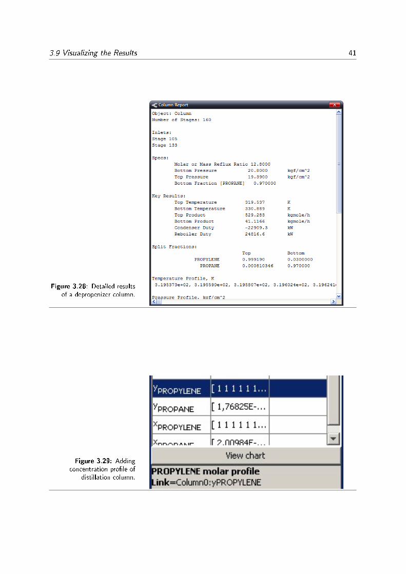
� with speci�c equipment reports (not available for all equip-ments, so far) as in Figure 3.28 for a distillation column.
� Using the interface with Microsoft Excel©, read ??.
After running a simulation the message "Results Available"is shown meaning that the values of the variables were updatedaccording to the simulation result.
Figure 3.27: Visualization ofthe top results of a
depropenizer column.
When a variable is actually a vector, like composition or columnpro�les, the result for these entities can be seen by selecting thetarget variable and clicking on the "view chart" button, as seen inFigure 3.29. A graphic, like the one of Figure 3.30 is generated.
3.9 Visualizing the Results 41
Figure 3.28: Detailed resultsof a depropenizer column.
Figure 3.29: Addingconcentration pro�le of
distillation column.

42 3 Creating Simulation Diagrams
Figure 3.30: Result ofconcentration pro�le in a
distillation column.

4 Water Steam Library
In this chapter the iiSE Water Steam Library is described. Each library has it's ownequipment set and physical chemical property data to build simulation diagrams.
Contents
4.1 Introduction . . . . . . . . . . . . . . . . . . . . . . . . . . . . . . 44
4.2 Streams . . . . . . . . . . . . . . . . . . . . . . . . . . . . . . . . . 45
4.3 Equipment Models . . . . . . . . . . . . . . . . . . . . . . . . . . . 47

44 4 Water Steam Library
4.1 Introduction
The Water Steam Library has the most common models fromenergy generation and co-generation industries based on waterand steam energy transfer. Currently available equipment modelsare shown in Figure 4.1.
Figure 4.1: Water Steam
Library equipments pallet.
When using the Water Steam Library, rigorous mass and en-ergy balances are taken into account in all equipments. A listeddescription of the models available is given in section 4.3.
Thermodynamic calculations are according to the International
Association for the Properties of Water and Steam (IAPWS) cor-relations, precise for industrial and scienti�c use [14]. The for-mulation is valid in the entire stable �uid region from the meltingcurve to 1273 K at pressures to 1000 MPa. Further, it extrap-olates in a physically reasonable way outside this region. Theprecision for di�erent regions is shown in Figure 4.2.
Remember that the Libraries should be selected by the user when

4.2 Streams 45
Figure 4.2: Precision of theIAPWS correlations [14]
availabe in iiSE.
creating a new project, as described in section 2.2. The user canselect more than one library for the same project but the materialstreams will only be compatible with streams of the same libraywhile energy streams are interchangeble. This allows, for instance,energy integration between processes based on di�erent libraries.
4.2 Streams
4.2.1 Material stream for water and steam
Material stream which can connect input and output materialports, contains the following variables:
Variable Description UOM
Mass Flowkgs
Temperature ◦CPressure MPa
Enthalpy kJkg
Entropy kJkg·K
This set of variables was chosen as a compromise between min-imal information and reduced recomputation of quantities when

46 4 Water Steam Library
an stream is shared between equipments. Thus, not all thesevariables are independent.
4.2.2 Energy Stream
Energy streams are an useful simpli�cation, since they are mentto represent any kind of energy (heat �ow, mechanical, electrical,etc.). Thus, energy streams are vey simple, holding only theinformation of the energy rate (or power) being exchanged.
While, in one hand, the energy streams provide great �exibility,on the other hand, there is no distinction between heat and workexchange.
Warning: According to the second law of thermodynamics, it isnot possible to fully convert heat in work, then special care shouldbe taken when using energy streams.

4.3 Equipment Models 47
4.3 Equipment Models
In this section all equipment models are described. Typical spec-i�cation sets are given for each model along with a brief modeldescription.
Tip: Although some speci�cations are advised in this manual,since iiSE is an equation-oriented simulator any other globallyfeasible speci�cation can be given.
For each model all variables available for speci�cation or inspec-tion in the iiSE user interface are also listed. Note that the modelscan have internal variables not listed here and not shown in theuser interface. These internal variables are hidden from the userto avoid unecessary confusion.
4.3.1 Source Saturated
Figure 4.3: Source Saturatedfrom Water Steam Library.
The following connection ports are available in this model:
Port Description TypeOutlet Material stream for water and steam pro-
cesses.output
This equipment provides a saturated water steam material stream.
Since the stream is assumed to be saturated, the temperature andpressure should not be speci�ed simultaneously.
The model have 3 local degrees of freedom. Usually the mass (orvolume) �owrate, pressure (or temperature) and vapor quality arespeci�ed.
This model contains the following visible variables:

48 4 Water Steam Library
Variable Description UOM
Mass Flowkgs
Temperature ◦C
Pressure MPa
Vapor quality (mass base) -
Volume Flow m3
sEnthalpy kJ
kg
Entropy kJkg·K
Speci�c masskgm3
4.3.2 Source
Figure 4.4: Source fromWater Steam Library.
The following connection ports are available in this model:
Port Description TypeOutlet Material stream for water and steam pro-
cesses.output
This equipment provides a water/steam material stream. All dif-ferent states are possible: compressed liquid (subcooled), super-heated (overheated) or saturated vapor
If the stream is saturated, please prefer the Source Saturatedmodel.
The model have 3 local degrees of freedom. Usually the mass (orvolume) �owrate, pressure and temperature are speci�ed.
This model contains the following visible variables:

4.3 Equipment Models 49
Variable Description UOM
Mass Flowkgs
Temperature ◦C
Pressure MPa
Volume Flow m3
sEnthalpy kJ
kg
Entropy kJkg·K
Speci�c masskgm3
4.3.3 Sink
Figure 4.5: Sink from Water
Steam Library.
The following connection ports are available in this model:
Port Description TypeInlet Material stream for water and steam pro-
cesses.input
This equipment provides a sink for a water/steam material stream.
This model is always optional, but it can be useful if the userwants to specify product properties instead of feed properties.For instance, specifying the sink �ow rate will make the simulator(if possible) to compute the other �ows as a function of it.
This model contains the following visible variables:
Variable Description UOM
Mass Flowkgs
Temperature ◦C
Pressure MPa
Enthalpy kJkg
Entropy kJkg·K
4.3.4 Source Sugar
The following connection ports are available in this model:

50 4 Water Steam Library
Figure 4.6: Source Sugarfrom Water Steam Library.
Port Description TypeOutlet Material stream for juice (water+sugar) output
This model contains the following visible variables:
Variable Description UOM
Mass Flowkgs
Mass Flowkgs
Mass Flowkgs
Volume Flow m3
sTemperature ◦C
Pressure MPa
Percent -
Fraction -
Fraction -
Enthalpy kJkg
Speci�c masskgm3
Enthalpy kJkg
Enthalpy kJkg
Enthalpy kJkg
4.3.5 Energy Source
Figure 4.7: Energy Sourcefrom Water Steam Library.
The following connection ports are available in this model:
Port Description TypeOutlet Outlet power (either heat or work) output
This equipment provides an energy stream.
Note that there is no distinction between heat and work energy

4.3 Equipment Models 51
sources. This equipment has only one variable and one localdegree of freedom (no equations). Usually the outlet energy isspeci�ed, e.g. zero for an adiabatic processes.
If this equipment is left unspeci�ed, it might get calculated by theenergy balance of the other equipment it is connected with.
This model contains the following visible variables:
Variable Description UOM
Outlet power (either heat or work) MW
4.3.6 Energy Source Gross HV
Figure 4.8: Energy SourceGross HV from Water Steam
Library.
The following connection ports are available in this model:
Port Description TypeOutletQ Power output
This equipment represents another energy source, but the amountof energy provided is computed as a function of the gross heatingvalue of a given fuel.
The resulting energy source can be used, for insance, to feed aboiler.
This model contains 3 local degrees of freedom. The user tipicallyspeci�es the fuel mass �ow, the gross heating value and e�ciency.
This model contains the following visible variables:
Variable Description UOM
Fuel mass �owkgs
Fuel gross heating value kJkg
Power MW
E�ciency (fraction of energy actuallyobtained)
-

52 4 Water Steam Library
Figure 4.9: Turbine fromWater Steam Library.
4.3.7 Turbine
The following connection ports are available in this model:
Port Description TypeInlet Material stream for water and steam pro-
cesses.input
Outlet Material stream for water and steam pro-cesses.
output
W Turbine Shaft Work output
This equipment represents a turbine, frequently used in vaporcycles for energy generation.
In this equipment, usually a steam stream is fed at high pressureand high temperature, discharging it at a lower pressure. Energyis converted in shaft work according to an isentropic e�ciency.
The model have 2 local degrees of freedom. Usually the pressureand e�ciency are speci�ed.
This model contains the following visible variables:
Variable Description UOM
Mass Flowkgs
Temperature ◦C
Pressure MPa
E�ciency (isentropic) -
Turbine Shaft Work MW
4.3.8 Turbine Bleeding
The following connection ports are available in this model:

4.3 Equipment Models 53
Figure 4.10: TurbineBleeding from Water Steam
Library.
Port Description TypeInlet Material stream for water and steam pro-
cesses.input
Outlet Material stream for water and steam pro-cesses.
output
Bleeding Material stream for water and steam pro-cesses.
output
W Turbine Shaft Work output
This model is a steam turbine with bleeding, where steam con-densation is considered.
This equipment extends the Turbine model, there is an additionaloulet material stream for condensed steam, named bleeding. Theenergy is converted in shaft work according to an isentropic e�-ciency.
This model has 3 local degrees of freedom, usually the pressure,e�ciency and bleeding are speci�ed.
This model contains the following visible variables:
Variable Description UOM
Mass Flowkgs
Temperature ◦C
Pressure MPa
E�ciency (isentropic) -
Bleeding mass fraction -
Turbine Shaft Work MW
4.3.9 Boiler
The following connection ports are available in this model:

54 4 Water Steam Library
Figure 4.11: Boiler fromWater Steam Library.
Port Description TypeInlet Material stream for water and steam pro-
cesses.input
Outlet Material stream for water and steam pro-cesses.
output
Q Boiler heat duty input
This equipment is a boiler used in water steam cicles to obtainhigh pressure steam by adding heat.
The boiler usually operates at a given pressure and temperature,fed by liquid water and discharging (usually) superheated (over-heated) steam.
The model has only 1 local degree of freedom. However, usuallythe pressure of operation is speci�ed as well as the temperature,the connected energy source is left unspeci�ed and is calculatedas a consequence.
This model contains the following visible variables:
Variable Description UOM
Boiler heat duty MW
Pressure MPa
Temperature ◦C
4.3.10 Evaporator
Figure 4.12: Evaporatorfrom Water Steam Library.

4.3 Equipment Models 55
The following connection ports are available in this model:
Port Description TypeInletVapor Material stream for water and steam pro-
cesses.input
OutletCondensate Material stream for water and steam pro-cesses.
output
OutletVapor Material stream for water and steam pro-cesses.
output
InletLiquor InletLiquor inputOutletLiquor Material stream for juice (water+sugar) output
This model contains the following visible variables:
Variable Description UOM
Temperature ◦C
Pressure MPa
Percent -
Evaporator heat duty MW
Area m2
Heat transfer coe�cient Wm2·K
Generic variable -
Pure water saturation temperature ◦C
Temperature elevation by concentration ∆◦C
4.3.11 Boiler Reheat
Figure 4.13: Boiler Reheatfrom Water Steam Library.
The following connection ports are available in this model:

56 4 Water Steam Library
Port Description TypeInlet Material stream for water and steam pro-
cesses.input
InletReheat Material stream for water and steam pro-cesses.
input
Outlet Material stream for water and steam pro-cesses.
output
OutletReheat Material stream for water and steam pro-cesses.
output
This equipment is a steam boiler with 2 heating stages, discharg-ing steam at 2 di�erent conditions. The main and second feedsare heated by the boiler but do not exchange mass with eachother.
Usually, the energy of the high pressure steam coming from themain feed is spent in the process and then comes back to the boilerto be re-heated, resulting in an intermediate pressure steam.
The model has 4 local degrees of freedom. The usual speci�ca-tions are the pressure and temperature of both stages.
This model contains the following visible variables:
Variable Description UOM
Total heat duty MW
Heat duty for the main stream MW
Heat duty for the re-heated stream MW
Outlet Flowkgs
Outlet Temperature ◦C
Outlet Pressure MPa
Reheated Flowkgs
Reheated Temperature ◦C
Reheated Pressure MPa
4.3.12 Pump
Figure 4.14: Pump fromWater Steam Library.
The following connection ports are available in this model:

4.3 Equipment Models 57
Port Description TypeInlet Material stream for water and steam pro-
cesses.input
Outlet Material stream for water and steam pro-cesses.
output
This equipment is a pump that adds energy to a material stream,increasing its pressure.
The pump is usually fed with sub-cooled (compressed liquid) wa-ter. Non-idealities are taken into account according to an isen-tropic e�ciency.
The model has 2 local degrees of freedom. Usually the pressure(or power) and e�ciency are speci�ed.
This model contains the following visible variables:
Variable Description UOM
Mass Flowkgs
Pressure MPa
Temperature ◦C
Pressure gain MPa
E�ciency -
Isentropic enthalpy kJkg
Potency MW
4.3.13 Condenser
Figure 4.15: Condenser fromWater Steam Library.
The following connection ports are available in this model:

58 4 Water Steam Library
Port Description TypeInlet Material stream for water and steam pro-
cesses.input
Outlet Material stream for water and steam pro-cesses.
output
Q Heat removed output
This equipment is a total condenser, a steam stream should begiven from which heat is removed. The equipment discharges asubcooled liquid stream.
The feed is usually an over-heated steam stream. In the con-denser, heat is removed until the steam becomes saturated, andthen subcooled.
The model has only 1 local degree of freedom, since zero pressuredrop is assumed in this equipment. The recomended speci�cationis the degree of subcooling, de�ned as the di�erence between thesaturation temperature and the current temperature for the givenpressure.
This model contains the following visible variables:
Variable Description UOM
Temperature ◦C
Pressure MPa
Enthalpy kJkg
Heat removed MW
Saturation temperature ◦C
Subcooling degree ∆◦C
4.3.14 Heater
Figure 4.16: Heater fromWater Steam Library.
The following connection ports are available in this model:

4.3 Equipment Models 59
Port Description TypeInlet Material stream for water and steam pro-
cesses.input
Outlet Material stream for water and steam pro-cesses.
output
Q Heat added input
A heater where a material stream is heated (or cooled) by anenergy stream. If the heat added is negative, it can act as acooler.
This model can be used in any process where heat is added or re-moved from a material stream in any state (subcooled, saturatedor superheated).
The model has only 1 local degree of freedom, however bothtemperature and pressure can be speci�ed if the energy stream isleft unspeci�ed.
This model contains the following visible variables:
Variable Description UOM
Heat added MW
Mass Flowkgs
Temperature ◦C
Pressure MPa
4.3.15 Heat Exchanger
Figure 4.17: Heat Exchangerfrom Water Steam Library.
The following connection ports are available in this model:

60 4 Water Steam Library
Port Description TypeInletCold Material stream for water and steam pro-
cesses.input
OutletCold Material stream for water and steam pro-cesses.
output
InletHot Material stream for water and steam pro-cesses.
input
outletHot Material stream for water and steam pro-cesses.
output
A heat exchanger model calculated by the LMTD method.
This model contains the following visible variables:
Variable Description UOM
Heat transfered from Hot to Cold MW
Heat Exchanger Area m2
Global Heat Transfer Coe�cient Wm2·K
Temperature Delta of input streams ∆◦C
Temperature Delta of output streams ∆◦C
Log Mean Temperature Delta ∆◦C
Hot Temperature ◦C
Hot Enthalpy kJkg
Hot Pressure MPa
Cold Temperature ◦C
Cold Enthalpy kJkg
Cold Pressure MPa
Saturation temperature ◦C
Subcooling degree ∆◦C
4.3.16 Mixer
Figure 4.18: Mixer fromWater Steam Library.

4.3 Equipment Models 61
The following connection ports are available in this model:
Port Description TypeInlet Material stream for water and steam pro-
cesses.input
Inlet2 Material stream for water and steam pro-cesses.
input
Outlet Material stream for water and steam pro-cesses.
output
This equipment is a simple mixer, the resulting stream is calcu-lated according to material and energy balances.
The model assumes that the resulting pressure is given by theminimum pressure of the inlet streams. The number of degreesof freedom is zero, then usually no speci�cation should be proviedin this model.
This model contains the following visible variables:
Variable Description UOM
Mass Flowkgs
Temperature ◦C
Pressure MPa
4.3.17 Splitter
Figure 4.19: Splitter fromWater Steam Library.
The following connection ports are available in this model:
Port Description TypeInlet Material stream for water and steam pro-
cesses.input
Outlet1 Material stream for water and steam pro-cesses.
output
Outlet2 Material stream for water and steam pro-cesses.
output
This equipment is a simple stream splitter, the resulting streamshave identical intensive properties (identical state) but possiblydi�erent �ow rates.
This model has 1 local degree of freedom, tipically the split frac-tion or the �ow rate of one of the outlet streams is speci�ed.

62 4 Water Steam Library
This model contains the following visible variables:
Variable Description UOM
Outlet1 split fraction -
Outlet1 Flowkgs
Outlet2 Flowkgs
Pressure MPa
Temperature ◦C
4.3.18 Recycle
Figure 4.20: Recycle fromWater Steam Library.
The following connection ports are available in this model:
Port Description TypeInlet Material stream for water and steam pro-
cesses.input
Outlet Material stream for water and steam pro-cesses.
output
This recycle equipment is an optional utility model for closedloop systems. This model is needed only when the process is fullyclosed (no material stream source or sink).
This is actually a side-e�ect of the equation-oriented method,since we have material balances in every other model, when thereis no source or sink, the model becomes singular, because anymass �ow rate would satify the model.
By using this model, the user will be able to specify the mass �owrate in closed loop systems, for instance in a Rankine cycle.
This model contains the following visible variables:
Variable Description UOM
Mass Flowkgs
Pressure MPa
Temperature ◦C

5 Process Engineering Library
In this chapter the iiSE Process Engineering Library is described. Each library has it'sown equipment set and physical chemical property data to build simulation diagrams.
Contents
5.1 Introduction . . . . . . . . . . . . . . . . . . . . . . . . . . . . . . 64
5.2 Thermodynamics . . . . . . . . . . . . . . . . . . . . . . . . . . . . 65
5.3 Streams . . . . . . . . . . . . . . . . . . . . . . . . . . . . . . . . . 75
5.4 Equipment Models . . . . . . . . . . . . . . . . . . . . . . . . . . . 77

64 5 Process Engineering Library
5.1 Introduction
The Process Engineering Library has several models for themost common equipments present in chemical and petrochemicalindustrial processes. The currently available equipment modelscan be seen in Figure 5.1.
Figure 5.1: ProcessEngineering Libraryequipments pallet.
Rigorous mass and energy balances are taken into account inall equipments. A listed description of the models available isgiven in section 5.4. Rigorous phase equilibria is also calculatedin several equipments, for more details on the thermodynamics,please check the section 5.2.

5.2 Thermodynamics 65
Remember that the Libraries should be selected by the user whencreating a new project, as described in section 2.2. The user canselect more than one library for the same project but the materialstreams will only be compatible with streams of the same libraywhile energy streams are interchangeble. This allows, for instance,energy integration between processes based on di�erent libraries.
5.2 Thermodynamics
When working with the Process Engineering Library, the �rststep is to select the chemical compounds to be considered in thesimulation. The iiSE database currently contains more than 1200compounds. In order to add the compounds to the simulation,
Please contact our support if yoursimulation needs a compound notpresent in the default database.
the user should search by compound name or formula, as can beseen in Figure 5.2.
Figure 5.2: Searching forcompounds.
The window shown in Figure 5.2 is always prompted when a newprocess �ow diagram is started with the Process EngineeringLibrary. At any moment the user can recon�gure the compo-nents or property models by selecting the Thermodynamicsbutton (�rst element in Figure 5.1).
For each compound in the database, several pure substance pa-rameters are available, as well as correlations and parameters for

66 5 Process Engineering Library
the prediction of real mixture behavior.
Each compound added will be considered in the simulation, be-ing one of the elements carried by the material streams. Afterthe compound selection, the user should con�gure the themo-dynamics model options to be used in the computations. Thisis accomplished by selecting the options present in the Modelstab, as shown in Figure 5.3.
Figure 5.3: Con�guring thethermodynamic models.
The �rst option is the Vapor as Ideal Gas check. If thisoption is selected, any vapor phase will be computed as an idealgas. This option can be used for low pressure systems or as aninitial attempt for di�cult to converge systems.
The ideal gas approximation usuallyagrees very well with experimentaldata for vapor phases below 5 atm.
The next step to be accomplished by the user is the selectionof the Equation of State/Package. Several equationsof state are available as well as special packages. More detailsare given in subsection 5.2.1 for cubic equations of state and insubsection 5.2.3 for the formaldehyde special package.
Depending on the equation selected, the user will be able to se-lect a mixing rule. Mixing rules can extend the applicability ofcubic equations of state to the prediction of high-pressure, high-temperature vapor-liquid equilibria of polar and/or asymmetricmixtures. The possibility to freely combine di�erent equations ofstate with di�erent mixing rules is a new concept in the processsimulation �eld. To the best of our knowledge, iiSE is the onlysimulator with support for this.

5.2 Thermodynamics 67
Warning: Although some directions on thermodynamic modelselection are given in this document, the user should always testthe model performance against experimental data.
Unless an ideal gas phase was selected, by default, the equation ofstate or package selected will compute both, gas and liquid phasebehavior. Optionally, the user can select a speci�c model for theactivity of liquid mixtures. By doing this, the liquid fugacities willbe computed by the activity model instead of using the equationof state.
Note: Since activity models do not take into account pressuree�ects, the Use Activity Model option should be selectedonly for low pressure systems. For high-pressure processes anequation of state combined with an advanced mixing rule shouldbe preferred.
The available activity models are detailed in subsection 5.2.2.
5.2.1 Cubic equations of state
When using the Process Engineering Library, several cubicequations of state are available:
PR : Peng-Robinson equation of state
SRK : Soave-Redlich-Kwong equation of state
SRK-MC : Soave-Redlich-Kwong equation of state with Mathias-Copemanconstants [12] for improved saturation pressures
RK : Redlich-Kwong equation of state
vdW : van der Waals equation of state
The RK and vdW equations of state usually do not produce goodquantitative results and should be used only for testing purposes.
Regarding pure �uids, the PR and SRK equations usually producevery good results for the vapor phase as well as good saturationtemperatures (pressures). One of the de�ciencies of these equa-tions is the poor prediction of liquid volumes. In a study with 91di�erent substances, the average error in the prediction of pure�uid liquid speci�c mass was 5.91 % for PR and 12.4 % for SRK[17].

68 5 Process Engineering Library
In order to improve the prediction quality for liquid volumes, theuser can make use of corrections known as volume translation.Currently two volume translation models are available:
VTPR : A temperature-dependent volume correction for the PR equa-tion of state. The average relative deviations for the 91 sat-urated pure compounds tested was as small as 1.37 %[17].The authors also tested the saturated liquid density of bi-nary mixtures with a relative deviation of 0.98 %.
Peneloux-ZRa : A correction to improve volume estimations with the SRKequation of state as described by [19]. The version imple-mented here is the one that uses the Rackett compressibilityfactor.
When dealing with mixtures, the performance of the cubic equa-tions of states is strongly dependent on the mixing rule selected.The mixing rules currently available for cubic equations of stateare described below.
vdW
In process simulators, although not clear to the user, the vdWmixing rule is typically used. Then, empirical binary interaction
parameters (BIPs) are needed for the description systems withsubstances dissimilar in size, shape and chemical nature.
Within iiSE the classic van der Waals mixing rule is referred simplyas vdW. When this option is active, no binary interaction param-eters are considered. Thus, the vdW mixing rule should be usedfor mixtures of small hydrocaborns only or if the simulation doesnot contain a liquid phase.
For some particular mixtures there are correlations for the pre-diction of binary interaction parameters (BIPs) available in theliterature. Within iiSE the cases available are:
vdW (HC-HC) : The most commonly used correlation for estimating BIPsof hydrocarbon-hydrocarbon (HC-HC) based on critical vol-umes [6]
vdW (H2-HC) : The correlations for hydrogen-hydrocarbon of Gray et. albased on critical temperatures [24], mainly for the predic-tion of hydrogen solubility in hydrocarbon mixtures
Advanced mixing rules, follow the idea of combining equations ofstate with activity coe�cient (Gibbs Excess) models [13]. Theycan extend the applicability of cubic equations of state to the pre-diction of high-pressure, high-temperature vapor-liquid equilibria

5.2 Thermodynamics 69
of polar and/or asymmetric mixtures. This concept is adopted iniiSE and several mixing rules are available, listed below:
PSRK
The predictive-SRK (PSRK) mixing rule [11]. This method shouldbe preferrably combined with the UNIFAC (PSRK) Gibbs Excessmodel. Currently, there is a great acceptance of PSRK, mainly ifgas related systems are considered [12].
UMR
The universal mixing rule (UMR) [22]. This mixing rule has someempirical modi�cations with the objective of improving predictionsfor asymmetric systems by eliminating the �double combinatoriale�ect� of the equation of state and Gibbs Excess model [16].Therefore, the method cannot be combined with any Gibbs Excessmodel, currenty the only option available is UNIFAC (PSRK).
MHV1
The modi�ed Huron-Vidal 1 (MHV1) mixing rule. One of themost famous mixing rules, enabling the application of cubic equa-tions of state to polar systems. Any Gibbs Excess model can becombined with this mixing rule. It is not recommended for mix-tures with molecules too dissimilar in size.
SCMR
The self-consistent mixing rule (SCMR) [21]. A recently proposedmixing rule which reproduce very well the low pressure behavior ofthe activity coe�cient it is coupled with as well as can be used inhigh-temperature and high-pressure conditions. Should be usedwith care, as it is a very recent model (2012).
5.2.2 Activity/Gibbs excess models
Activity coe�cient models and Gibbs excess models are usuallytaken as synonyms, since one quantity can be computed from theother by standard thermodynamic relations. In the iiSE simula-tor, these models are referred as Gibbs excess models (ge) in thecontext of mixing rules. When using these models for directlycomputing the fugacities of liquid phases, they are referred asactivity models.
The activity/Gibbs excess models currently available are:

70 5 Process Engineering Library
UNIFAC (Do)
The famous modi�ed UNIFAC, with parameters from a series ofsources [7, 8, 9, 18, 15]. Care should be taken for molecules withmore then one functional group other than hydrocarbon groups.
UNIFAC (PSRK)
A modi�ed UNIFAC model with parameters specially �tted to beused with the PSRK mixing rule [12]. Although the model wascalibrated with the PSRK mixing rule, good results are also oftenobtained when using this model alone (as an activity coe�cientmodel) or when this model is combined with other mixing rules.
Scatchard-Hildebrand
Scatchard-Hildebrand regular solution activity coe�cient modelwith parameters for hydrocarbons and some other common com-pounds in the petroleum industry (light gases and water). Thismodel is predictive in the sense that mixture behavior can becalculated from pure properties only. This model is used in theclassical Chao-Seader method. In iiSE this model can be selectedin association with the SCMR mixing rule in order to simulatepetroleum fractionation processes, see also subsection 5.2.4. Thismethod will predict separate water and oil phases. The water richphase will be nearly pure water and a small water solubility ofwater in oil is predicted.
IdealLiquid
This package assumes an ideal liquid mixture � unitary activitycoe�cients for all substances in mixture. The behavior will beidentical to the Raoult's law if this model is selected for the ac-tivity of the liquid phase and if an ideal gas is selected for thevapor phase.
5.2.3 FA-ME-W Package
The FA-ME-W is a special package for modeling mixtures offormaldehyde (FA), methanol (ME), and water (W). Formalde-hyde is a very important intermediate industrial chemical. Model-ing the thermodynamic properties of formaldehyde solutions hasbeen a research topic of several groups for many years [3].
Because formaldehyde is highly reactive, it is not possible to storeit as a pure substance. Then, it is usually stabilized in binary solu-tions with water. Methanol can also be present (added or formed

5.2 Thermodynamics 71
during the reaction process). With methanol, the amount of watercan be reduced as the solubility of formaldehyde in an aqueousphase is enhanced. Therefore, it is necessary to take into ac-
However, at low temperaturessmall amounts of methanol may
result in a considerable increase inthe volatility of formaldehyde [10].
count the strong interactions in the ternary system formaldehyde-methanol-water.
Mixtures of formaldehyde with methanol or with water are notbinary in the usual sense, since they react to form a variety ofproducts. Several investigations have shown that solutions offormaldehyde (FA) and methanol (ME) react to form hemiformal(HF) and poly-oxymethylene hemiformals (HFn) while solutionsof FA and water (W) react to form methylene glycol (MG) andpoly-oxymethylene glycols (MGn), as follows:
FA + ME −−⇀↽−− MG
MGn−1 + MG −−⇀↽−− MGn + ME (n ≥ 2)
FA + W −−⇀↽−− HF
HFn−1 + HF −−⇀↽−− HFn + W (n ≥ 2)
(5.1)
All these reaction products are taken into account by the iiSEpackage known as FA-W-ME Package. Actually, if using thispackage, before any computation the true composition accordingto the reactions in Equation 5.1 is determined. The user does notneed to worry about true compostion in terms of hemiformals(HF and HFn) and methylene glycols (MG and MGn), becauseonly the apparent compostions in terms of the original quantities(FA, ME, and W) are exposed to the user.
Typical results, in comparision with experimental data of vapor-liquid equilibrium (VLE), are shown in Figure 5.4 for ME-W, inFigure 5.5 for FA-ME and Figure 5.6 for FA-W.
Figure 5.4: Methanol-waterVLE, exp. data from [2].

72 5 Process Engineering Library
Figure 5.5:
Formaldehyde-methanol VLE,exp. data from [10].
Figure 5.6:
Formaldehyde-water VLE,exp. data from [4].
The vapor phase behavior is corrected by considering an idealgas mixture in terms of the true compostion resulting from thechemical equilibrium given by Equation 5.1. By assuming this,good agreement with experimental data is expected for pressuresbelow 5 atm.
For the liquid phase, the real interaction between the true speciesis taken into account by a speci�cally calibrated UNIFAC model.Good agreement with experimental data is obtained for temper-atures ranging from 292 to 413 K and for (apparent) molar con-centrations of formaldehyde below 40% [3].
Liquid volumes are computed by the Rackett [23] correlation withspecially �tted parameters for pure �uid liquid volumes. Mixturee�ects are ignored when computing the liquid volumes (zero ex-cess volume). Heat of mixture e�ects, on the other hand, areconsidered [3].
Good predictions are also obtained by the FA-W-ME Packagefor ternary mixtures of formaldehyde-methanol-water, with errors

5.2 Thermodynamics 73
below 5% in pressure and compostions, as reported by [3].
Compounds other than formaldehyde, methanol, and water canalso be present in the mixture but good results are expected onlyif these other compounds are inert in the system and are presentin small amounts in the liquid phase. This is the case of lightgases like H2, N2, O2, etc.
5.2.4 Petroleum modeling
Petroleum fractions are mixtures of countless hydrocarbon com-pounds from di�erent families. Thus, the determination of theexact composition of all components existing in the mixtures be-comes impractical. For this reason, a limited number of com-pounds that best represent the mixture behavior is used. Theselimited compounds are di�erent from the real ones in mixtureand are known as pseudocomponents. Once a list of pseudo-components and its composition is determined, the simulation isaccomplished as usual.
In order to con�gure a petroleum the user should open the thermo-dynamics dialog (see section 5.2) and then select Oil manager...,as shown in Figure 5.7
Figure 5.7: Opening the oilmanager dialog.
Once the oil manager dialog is opened, the �rst thing to do is tocreate a new oil.
A just created oil is shown in Figure 5.8. The Assay name isused in all future references of this oil and should be unique inthe simulation. The other con�guration �elds should be �lled asdescribed in the bottom left portion of the dialog.
The user should provide at least a distillation curve experiment.True boiling point (TBP) experiments are more reliable but ASTM

74 5 Process Engineering Library
D86 curves are also allowed. As more information is provided,more reliable pseudocomponents are generated.
Figure 5.8: Con�guring anew oil, �ll the �elds as
described in the bottom leftdetails.
Instead of entering manually the assay data, the user can also im-port data from other databases by using the Import... button.Currently only Petrobras BDAP import is supported. After thedata is successfully imported the user can add/correct the assaydata.
With a distillation curve (and preferrably more) data added, theuser should check how the statistical distribution model proposedby Riazi [1] �t the data by selecting the Check fit button.Typical results are shown in Figure 5.9.
If a poor �t is observed the user should double check the distil-lation data. If the user considers the �t good enouth, the pseu-docomponents can be genarated by selecting the Cut Assaybutton.
As can be seen in Figure 5.9, light compounds are also iden-ti�ed. Pseudocompounds are created only for compounds withmore than 5 carbons. For light gases and hydrocarbons until N-PENTANE real components are used. Experimental light endscan be informed (preferred) as well as automatically generatedfrom the distillation curve data. When experimental light endsare added, a smoth transition from the lights to the pseudocom-ponents should be observed. Otherwise, the user should doublecheck both the experimental light end values as well as the distil-lation curve data.
In order to actually use the oil in a simulation the user should in-

5.3 Streams 75
Figure 5.9: Oil con�guredand installed, with
pseudocomponents and lightsidenti�ed.
stall the created pseudocomponents by means of the Installbutton. Once installed the oil pseudocomponents cannot be al-tered untill it is uninstalled. The resulting oil composition in termsof the lights and created pseudocomponents can be imported intoany material stream source object. The user just need to select amaterial stream source and edit the composition (molar or mass).When editing the composition a dialog as shown in the Figure 5.10is be prompted. The user can then import the composition fromany installed oil by clicking the From Oil... button.
Figure 5.10: Material streamcomposition from oil.
5.3 Streams
5.3.1 Material stream
Material stream which can connect input and output materialports, contains the following variables:

76 5 Process Engineering Library
Variable Description UOM
Molar Flowkgmole
hTemperature ◦CPressure atm
Enthalpy Jgmole
Vapour fraction -Overall molar composition -
This set of variables was chosen as a compromise between min-imal information and reduced recomputation of quantities whenan stream is shared between equipments. Thus, not all thesevariables are independent.
Note: Some streams may carry more information than the statedabove. For instance, molar compostions of the liquid and vaporphases besides the overall composition.
Source and sink streams also contain the standard ideal liquid vol-ume �ow. This is the volumetric �ow at 15.5 C (60 F) of the idealliquid, i.e. without mixing e�ects (zero excess volume). For lighthydrocarbons like CH4, an apparent liquid volume is assumed, asdescribed either in ASTM D2421 [5] or in GPSA engineering databook. For substances with density data at conditions other thanthe standard ones, the pure liquid volume is extrapolated to thestandard conditions by the Rackett correlation [23].
5.3.2 Energy Stream
Energy streams are an useful simpli�cation, since they are mentto represent any kind of energy (heat �ow, mechanical, electrical,etc.). Thus, energy streams are vey simple, holding only theinformation of the energy rate (or power) being exchanged.
While, in one hand, the energy streams provide great �exibility,on the other hand, there is no distinction between heat and workexchange.
Warning: According to the second law of thermodynamics, it isnot possible to fully convert heat in work, then special care shouldbe taken when using energy streams.

5.4 Equipment Models 77
5.4 Equipment Models
5.4.1 Source
Figure 5.11: Source fromProcess Engineering
Library.
The following connection ports are available in this model:
Port Description TypeOutlet Process engineering material stream output
This equipment provides a material stream as its outlet.
The model has 3+C local degrees of freedom. The usual speci�-ation consists in the �ow rate (molar, mass or volume), tempera-ture, pressure and composition (mass or molar). If the simulationcontains one or more oils con�gured, the composition can be im-ported from the oil manager.
This model contains the following visible variables:
Variable Description UOM
Molar Flowkgmole
hMass Flow
kgh
Volumetric Flow m3
hTemperature ◦C
Pressure atm
Enthalpy Jgmole
Vapour fraction -
Molar composition -
Mass composition -
Average molecular weightg
gmole
5.4.2 Sink
The following connection ports are available in this model:
Port Description TypeInlet Process engineering material stream input
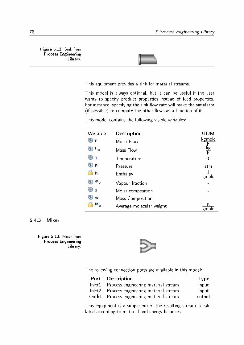
78 5 Process Engineering Library
Figure 5.12: Sink fromProcess Engineering
Library.
This equipment provides a sink for material streams.
This model is always optional, but it can be useful if the userwants to specify product properties instead of feed properties.For instance, specifying the sink �ow rate will make the simulator(if possible) to compute the other �ows as a function of it.
This model contains the following visible variables:
Variable Description UOM
Molar Flowkgmole
hMass Flow
kgh
Temperature ◦C
Pressure atm
Enthalpy Jgmole
Vapour fraction -
Molar composition -
Mass Composition -
Average molecular weightg
gmole
5.4.3 Mixer
Figure 5.13: Mixer fromProcess Engineering
Library.
The following connection ports are available in this model:
Port Description TypeInlet1 Process engineering material stream inputInlet2 Process engineering material stream inputOutlet Process engineering material stream output
This equipment is a simple mixer, the resulting stream is calcu-lated according to material and energy balances.

5.4 Equipment Models 79
The model assumes that the resulting pressure is given by theminimum pressure of the inlet streams. The number of degreesof freedom is zero, then usually no speci�cation should be proviedin this model.
This model contains the following visible variables:
Variable Description UOM
Molar Flowkgmole
hTemperature ◦C
Pressure atm
5.4.4 Mixer3
Figure 5.14: Mixer3 fromProcess Engineering
Library.
The following connection ports are available in this model:
Port Description TypeInlet1 Process engineering material stream inputInlet2 Process engineering material stream inputInlet3 Process engineering material stream inputOutlet Process engineering material stream output
This equipment is a simple mixer, but with 3 inlet ports. Theresulting stream is calculated according to material and energybalances.
The model assumes that the resulting pressure is given by theminimum pressure of the inlet streams. The number of degreesof freedom is zero, then usually no speci�cation should be proviedin this model.
This model contains the following visible variables:
Variable Description UOM
Molar Flowkgmole
hTemperature ◦C
Pressure atm

80 5 Process Engineering Library
5.4.5 Splitter
Figure 5.15: Splitter fromProcess Engineering
Library.
The following connection ports are available in this model:
Port Description TypeInlet1 Process engineering material stream inputOutlet1 Process engineering material stream outputOutlet2 Process engineering material stream output
This equipment is a simple stream splitter, the resulting streamshave identical intensive properties (identical state) but possiblydi�erent �ow rates.
This model has 1 local degree of freedom, tipically the split frac-tion or the �ow rate of one of the outlet streams is speci�ed.
This model contains the following visible variables:
Variable Description UOM
Temperature ◦C
Pressure atm
Outlet1 fraction -
Outlet 1 molar �owkgmole
hOutlet 2 molar �ow
kgmoleh
Outlet 1 mass �owkgh
Outlet 2 mass �owkgh
Average molecular weightg
gmole
5.4.6 Energy Source
Figure 5.16: Energy Sourcefrom Process Engineering
Library.
The following connection ports are available in this model:

5.4 Equipment Models 81
Port Description TypeOutlet Outlet energy stream output
This equipment provides an energy stream.
Note that there is no distinction between heat and work energysources. This equipment has only one variable and one localdegree of freedom (no equations). Usually the outlet energy isspeci�ed, e.g. zero for an adiabatic processes.
If this equipment is left unspeci�ed, it might get calculated by theenergy balance of the other equipment it is connected with.
This model contains the following visible variables:
Variable Description UOM
Outlet energy stream kW
5.4.7 Energy Source Gross HV
Figure 5.17: Energy SourceGross HV from Process
Engineering Library.
The following connection ports are available in this model:
Port Description TypeOutletQ Outlet energy stream output
This equipment represents another energy source, but the amountof energy provided is computed as a function of the gross heatingvalue of a given fuel.
The resulting energy source can be used, for insance, to feed aboiler.
This model contains 3 local degrees of freedom. The user tipicallyspeci�es the fuel mass �ow, the gross heating value and e�ciency.
This model contains the following visible variables:

82 5 Process Engineering Library
Variable Description UOM
Mass Flowkgs
Gross Heating Value kJkg
Outlet energy stream MW
E�ciency -
5.4.8 Energy Splitter
Figure 5.18: Energy Splitterfrom Process Engineering
Library.
The following connection ports are available in this model:
Port Description TypeInlet1 Inlet energy stream. inputOutlet1 Outlet 1 energy stream. outputOutlet2 Outlet 2 energy stream. output
This is an energy splitter to be used when an energy source willbe used in more than one equipment.
Note that there is no distinction between heat and work energystreams.
This model contains only 1 local degrees of freedom. The usertipically speci�es the split fraction or the one of the outlet powers.
This model contains the following visible variables:
Variable Description UOM
Inlet energy stream. kW
Outlet 1 energy stream. kW
Outlet 2 energy stream. kW
Outlet 1 fraction -
Outlet 2 fraction -
5.4.9 Flash
The following connection ports are available in this model:

5.4 Equipment Models 83
Figure 5.19: Flash fromProcess Engineering
Library.
Port Description TypeInlet Process engineering material stream input
OutletV Process engineering material stream outputOutletL Process engineering material stream outputInletQ Heat Input input
A standard �ash drum for vapor-liquid equilibrium.
This model contains only 1 local degree of freedom, consideringan speci�ed energy inlet stream. Usually, the energy inlet streamis left unspeci�ed, then 2 speci�cations are given in the �ash, forinstance: temperature and pressure, temperature and vaporiza-tion fraction, etc. If the inlet energy stream is missing, then the�ash is adiabatic.
This model contains the following visible variables:
Variable Description UOM
Heat Input kW
Temperature ◦C
Pressure atm
Liquid Molar Flowkgmole
hVapour Molar Flow
kgmoleh
Vaporization fraction -
Pressure drop with respect to the inletpressure
atm
Pressure drop ratio with respect to theinlet pressure
-

84 5 Process Engineering Library
5.4.10 FlashPH
Figure 5.20: FlashPH fromProcess Engineering
Library.
The following connection ports are available in this model:
Port Description TypeInlet Process engineering material stream input
OutletV Process engineering material stream outputOutletL Process engineering material stream outputInletQ Heat Input input
A �ash drum for vapor-liquid equilibrium similar to the Flashmodel, but with a di�erent algorithm.
The behavior is identical to the standard Flash but this modeluses an pressure-enthalpy algorithm.
This model contains the following visible variables:
Variable Description UOM
Heat Input kW
Temperature ◦C
Pressure atm
Liquid Molar Flowkgmole
hVapour Molar Flow
kgmoleh
Vaporization fraction -
Pressure drop ratio with respect to theinlet pressure
-
Pressure drop with respect to the inletpressure
atm
Enthalpy Jgmole

5.4 Equipment Models 85
5.4.11 Flash-VLL
Figure 5.21: Flash-VLL fromProcess Engineering
Library.
The following connection ports are available in this model:
Port Description TypeInlet Process engineering material stream input
OutletV Process engineering material stream outputOutletL Process engineering material stream outputOutletL2 Process engineering material stream outputInletQ Heat Input input
A �ash drum for vapor-liquid-liquid equilibrium.
This model contains only 1 local degree of freedom, consideringan speci�ed energy inlet stream. Usually, the energy inlet streamis left unspeci�ed and the user speci�es the �ash temperature andpressure. If the inlet energy stream is missing, then the �ash isadiabatic.
This model contains the following visible variables:

86 5 Process Engineering Library
Variable Description UOM
Heat Input kW
Temperature ◦C
Pressure atm
Vapour Molar Flowkgmole
hLiquid Molar Flow
kgmoleh
Liquid2 Molar Flowkgmole
hVaporization fraction -
Liquid 1 fraction -
Liquid 2 fraction -
5.4.12 Column
Figure 5.22: Column fromProcess Engineering
Library.
The following connection ports are available in this model:
Port Description Typefeed1 Process engineering material stream input
TopProduct Process engineering material stream outputBottomProduct Process engineering material stream output
A rigorous distillation column model. Thermodynamic equilibriumis assumed in each stage and the model contains the so calledMESH equations. The model can be used for tray or packedcolumns as long as the number of theoretical stages is known.

5.4 Equipment Models 87
Multiple feed and product streams can be added as well as mul-tiple column con�gurations by selecting the presence or not of acondenser and reboiler.
If no condenser and no reboiler are selected, then there are zerodegrees of freedom and the user should add feed streams to the�rst (top) and last tray (bottom). Each side stream adds an addi-tional degree of freedom and its �owrate is usually speci�ed. For astandard distillation column, a typical speci�cation set consists inthe re�ux rate and top product �ow rate. Several other combina-tions of speci�cations are also possible, including the composition(purity) of a component on top or bottom.
This model contains the following visible variables:
Variable Description UOM
Molar or Mass Re�ux ratio -
Distillate molar �ow ratekgmole
hBottom molar �ow rate
kgmoleh
Distillate Temperature ◦C
Bottom Temperature ◦C
Column top pressure. atm
Column bottom pressure. atm
Pressure drop per stage. atm
Condenser heat duty. kW
Reboiler heat duty. kW
Distillate molar �ow composition -
Bottom molar �ow composition -
Temperature pro�le ◦C
for each compound COMP, molar pro�le -
for each compound COMP, molar pro�le -
5.4.13 Separator
The following connection ports are available in this model:
Port Description TypeInlet1 Process engineering material stream inputOutlet1 Process engineering material stream outputOutlet2 Process engineering material stream output
This model contains the following visible variables:

88 5 Process Engineering Library
Figure 5.23: Separator fromProcess Engineering
Library.
Variable Description UOM
Temperature ◦C
Pressure atm
Top molar �owkgmole
hBottoms molar �ow
kgmoleh
Top mass �owkgh
Bottoms mass �owkgh
Top molar composition -
Bottoms molar composition -
Overall top molar or mass fraction -
Top split fraction -
5.4.14 Compressor
The following connection ports are available in this model:
Port Description TypeInlet Process engineering material stream input
OutletV Process engineering material stream outputW Compressor work duty input
A model for compressing gas streams by means of mechanicalwork.

5.4 Equipment Models 89
Figure 5.24: Compressorfrom Process Engineering
Library.
This model assumes that the inlet and outlet streams contain noliquid. Mechanical work is used in order to compress the �uid.Mass and energy balances are applied and an isentropic e�ciencyis considered. For proper functioning an inlet energy stream mustbe connected.
The model has only 1 local degrees of freedom. But, usually, theinlet energy stream is left unspeci�ed and then the pressure ande�ciency are speci�ed on this equipment.
This model contains the following visible variables:
Variable Description UOM
Molar Flowkgmole
hTemperature ◦C
Pressure atm
Molar composition -
Pressure gain atm
Isentropic e�ciency -
Isentropic temperature ◦C
Isentropic enthalpy Jgmole
Compressor work duty kW
5.4.15 Turbine
Figure 5.25: Turbine fromProcess Engineering
Library.

90 5 Process Engineering Library
The following connection ports are available in this model:
Port Description TypeInlet Process engineering material stream input
OutletV Process engineering material stream outputW Turbine shaft work output
A model for a gas turbine, producing mechanical work from ahigh pressure �uid.
This model assumes that the inlet and outlet streams containno liquid. Mechanical work is obtained from the �uid. Massand energy balances are applied and an isentropic e�ciency isconsidered.
The model has 2 local degrees of freedom, usually the pressureand e�ciency are speci�ed.
This model contains the following visible variables:
Variable Description UOM
Molar Flowkgmole
hTemperature ◦C
Pressure atm
Molar composition -
Pressure drop atm
Isentropic e�ciency -
Isentropic temperature ◦C
Isentropic enthalpy Jgmole
Turbine shaft work kW
5.4.16 Pump
Figure 5.26: Pump fromProcess Engineering
Library.
The following connection ports are available in this model:
Port Description TypeInlet Process engineering material stream inputOutlet Process engineering material stream output

5.4 Equipment Models 91
This is the model for a pump, converting mechanical work into�uid pressure.
This model assumes that the inlet and outlet streams are com-pressed (subcooled) liquids. Mechanical work is converted into�uid pressure according to an isentropic e�ciency. Mass and en-ergy balances are also applied.
The model has only 1 local degree of freedom. But, usually, theinlet energy stream is left unspeci�ed and then the pressure ande�ciency are speci�ed on this equipment.
This model contains the following visible variables:
Variable Description UOM
Molar Flowkgmole
hTemperature ◦C
Pressure atm
Pressure gain atm
Isentropic E�ciency -
Pump work duty kW
5.4.17 Equilibrium Reactor
Figure 5.27: EquilibriumReactor from Process
Engineering Library.
The following connection ports are available in this model:
Port Description TypeInlet Process engineering material stream inputOutlet Process engineering material stream outputInletQ Heat Input input
A model for gas phase thermodynamic equilibrium reaction.

92 5 Process Engineering Library
In this model a single reaction in gas phase is assumed. Thereaction stoichiometry is given by the user and then the thermo-dynamic equilibrium, according to standard formation properties,is calculated.
The model has only 1 local degree of freedom. But, usually, theinlet energy stream is left unspeci�ed and then the pressure andtemperature are speci�ed on this equipment.
This model contains the following visible variables:
Variable Description UOM
Heat Input kW
Heat of reaction at the reaction temper-ature
Jgmole
Molar Flowkgmole
hTemperature ◦C
Pressure atm
Molar composition -
Fugacity coe�cient of the compounds inmixture
-
Reaction stoichiometry -
Equilibrium Constant -
Ideal gas Gibbs energy of formation Jgmole
Ideal gas enthalpy of formation Jgmole
Reaction Advancekgmole
h
5.4.18 Gibbs Reactor
Figure 5.28: Gibbs Reactorfrom Process Engineering
Library.

5.4 Equipment Models 93
The following connection ports are available in this model:
Port Description TypeInlet Process engineering material stream inputOutlet Process engineering material stream outputInletQ Reactor Heat Duty input
A model for gas phase thermodynamic equilibrium reaction byGibbs energy minimization.
In this model, all possible reactions in gas phase are taken intoaccount. Thus, no stoichiometry need to be informed. The re-sulting composition is given by the thermodynamic equilibrium,according to standard formation properties when all possible re-actions between the compounds in mixture are considered.
The model has only 1 local degree of freedom. But, usually, theinlet energy stream is left unspeci�ed and then the pressure andtemperature are speci�ed on this equipment.
This model contains the following visible variables:
Variable Description UOM
Reactor Heat Duty kW
Total heat of reaction at the reactor tem-perature
kW
Molar Flowkgmole
hTemperature ◦C
Pressure atm
Molar composition -
5.4.19 Stoichiometric Reactor
Figure 5.29: StoichiometricReactor from Process
Engineering Library.

94 5 Process Engineering Library
The following connection ports are available in this model:
Port Description TypeInlet Process engineering material stream inputOutlet Process engineering material stream outputInletQ Heat input input
A simple reactor with known reaction stoichiometry.
This model can be used for liquid and gas phase reaction as wellas for mixed liquid-vapor mixtures. The reaction stoichiometry isgiven by the user and no reaction equilibrium is assumed. Thereaction extent and conversion are constrained by mass balances.
The model has 2+C local degrees of freedom. A typical speci�-cation consists in the stoichiometric coe�cients for the C com-pounds, the pressure and the conversion. Additionaly, the tem-perature can also be speci�ed if the inlet energy stream is leftunspeci�ed.
This model contains the following visible variables:
Variable Description UOM
Heat input kW
Molar Flowkgmole
hTemperature ◦C
Pressure atm
Molar composition -
Reaction stoichiometry -
Conversion with respect to for each com-pound COMP,
-
Extent of Reactionkgmole
hStandard heat of reaction at the reactiontemperature
Jgmole
Standard enthalpy of formation at the re-action temperature
Jgmole
5.4.20 Heat Exchanger
The following connection ports are available in this model:

5.4 Equipment Models 95
Figure 5.30: Heat Exchangerfrom Process Engineering
Library.
Port Description TypeInletCold Process engineering material stream inputOutletCold Process engineering material stream outputInletHot Process engineering material stream inputoutletHot Process engineering material stream output
A heat exchanger model calculated according to the LMTDmethod.
This model contains the following visible variables:
Variable Description UOM
Heat transfered from Hot to Cold MW
Heat Exchanger Area m2
Global Heat Transfer Coe�cient Wm2·K
Temperature Delta of input streams ∆◦C
Temperature Delta of output streams ∆◦C
Log Mean Temperature Delta ∆◦C
Hot outlet temperature ◦C
Hot outlet enthalpy Jgmole
Hot outlet pressure atm
Cold outlet temperature ◦C
Cold outlet enthalpy Jgmole
Cold outlet pressure atm
5.4.21 Heater
The following connection ports are available in this model:
Port Description TypeInlet Process engineering material stream inputOutlet Process engineering material stream outputInletQ Heat Input input

96 5 Process Engineering Library
Figure 5.31: Heater fromProcess Engineering
Library.
The model for a heater where a material stream is heated by anenergy stream.
If the inlet energy stream is actually negative, the the model willbehave as a cooler.
The model has only 1 local degree of feedom. Typically the pres-sure drop is speci�ed. If the inlet energy stream is unspeci�ed,then both temperature and pressure can be speci�ed in this equip-ment.
This model contains the following visible variables:
Variable Description UOM
Heat Input kW
Molar Flowkgmole
hTemperature ◦C
Pressure atm
Molar composition -
Pressure drop atm
5.4.22 Cooler
Figure 5.32: Cooler fromProcess Engineering
Library.
The following connection ports are available in this model:

5.4 Equipment Models 97
Port Description TypeInlet Process engineering material stream inputOutlet Process engineering material stream outputOutletQ Heat Output output
The model for a cooler where a material stream is cooled, resultingin an energy stream.
If the outlet energy stream is actually negative, the the model willbehave as a heater.
The model has 2 local degrees of feedom. Typically the pressuredrop and the temperature (or heat)are speci�ed.
This model contains the following visible variables:
Variable Description UOM
Heat Output kW
Molar Flowkgmole
hTemperature ◦C
Pressure atm
Molar composition -
Pressure drop atm
5.4.23 Recycle
Figure 5.33: Recycle fromProcess Engineering
Library.
The following connection ports are available in this model:
Port Description TypeInlet Process engineering material stream inputOutlet Process engineering material stream output
This recycle equipment is an optional utility model for closedloop systems. This model is needed only when the process is fullyclosed (no material stream source or sink).
This is actually a side-e�ect of the equation-oriented method,since we have material balances in every other model, when thereis no source or sink, the model becomes singular, because anymass �ow rate would satify the model.

98 5 Process Engineering Library
By using this model, the user will be able to specify the mass �owrate in closed loop systems, for instance in a Rankine cycle.
This model contains the following visible variables:
Variable Description UOM
Molar Flowkgmole
hTemperature ◦C
Pressure atm
Molar composition -
5.4.24 Valve
Figure 5.34: Valve fromProcess Engineering
Library.
The following connection ports are available in this model:
Port Description TypeInlet Process engineering material stream inputOutlet Process engineering material stream output
This is the model for a process valve operating with liquid streams.
The model is considered adiabatic and the valve intruduces apressure drop into the �uid. The �ow coe�cient is computedassuming liquid �ow only and no viscosity correction is applied aswell as no �ashing or cavitation are considered.
The model has 2 local degrees of feedom. Typical speci�cation isgiven by the pressure and valve �ow coe�cient.
This model contains the following visible variables:

5.4 Equipment Models 99
Variable Description UOM
Valve pressure drop atm
Pressure drop ratio with respect to theinlet pressure
-
Valve opening fraction (linear valve) -
Volumetric Flow m3
hValve �ow coe�cient, GPM when fullyopened at 60 F for 1 psi of pressure drop
-
Speci�c gravity (with respec to to waterat 60 F)
-
Speci�c masskgm3
Speci�c volume m3
gmole

6 Interfaces with other software
In this Chapter the several iiSE interfaces with other sotware are presented. Currently thereare ready to use interfaces for Microsoft Excel©, Scilab, Matlab, Java and Python.
Using the Java interface through JNI, C/C++ code can also make use of the iiSE simulationengine and thermodynamics server.

6.1 Variable links 101
6.1 Variable links
In order to identify the iiSE simulation variables in the severalinterfaces for other software each variable has a unique Link.
In order to discover the link of a variable, the user must select thedesired equipment in the diagram, then select the variable in theVariables panel. The Link will be shown at the very bottomof the Variables panel, as shown in Figure 6.1.
Figure 6.1: Identifying avariable Link in iiSE.
For the example shown in Figure 6.1, the turbine shaft work isidenti�ed by the link Turbine:W. This Link can be used in allinterfaces with other software in order to either change speci�ca-tion values or retrieve simulation values.
Note: For this particular example, since the shaft work is notbeing speci�ed in the simulation it will not be possible to changeits speci�cation value.
6.2 Microsoft Excel©Add-in
The results of a iiSE simulation can be retrieved by MicrosoftExcel© using the iiSE add-in. It is also possible to modify speci-�cation values, run simulations and retrieve results.

102 6 Interfaces with other software
Firstly, the iiSE simulator must be opened and the process �owdiagram of interest simulated with success. To start the iiSE- Microsoft Excel© interface, the user have to select the menuConfigurations, and then Excel Link, as shown in Fig-ure 6.2. After, it is necessary to open the iiseXLL.xll add-in,found in the iiSE installation folder, as shown in Figure 6.3.
Figure 6.2: StartingMicrosoft Excel©
communication with iiSE .
Figure 6.3: Locating thecommunication add-in.
After the add-in is opened a message like the one in Figure 6.4will be shown. Choose the option Enable this add-in (or similarin your language).
Figure 6.4: Enabling ISEXLLplugin message.
Once the add-in is enabled, the user can create a spreadsheet tocapture the iiSE simulation results as well as modify speci�ca-

6.2 Microsoft Excel©Add-in 103
tions and run new simulations. There iiSE add-in provides somefunctions to be used in Microsoft Excel© spreadsheets. The func-tion iise.desc retrieves a variable description. The functioniise.value returns a variable value. These functions can beused freely in Microsoft Excel© cells as follows:
=iise.desc("Link")=iise.value("Link";"UOM")
The Link is the variable unique identi�er (see section 6.1) andUOM is the desired unit of measurement for the given variable.
Both arguments, Link and UOM, must be identi�ed using doublequotes " " since they are strings. It is also important to em-phasize that the equal sign = is mandatory before the functioncalling.
For example, if the turbine shaft work is identi�ed by the linkTurbine:W, then this variable value can be retrieved in Mi-crosoft Excel© with the following command:
=iise.value("Turbine:W";"MW")
Naturally, the Link and UOM can also come from di�erent cellsby using standard cell references:
=iise.desc(A9)=iise.value(A9;B9)
where A9 contains the text of the variable link and B9 the UOM.
Warning: Always run a simulation before retrieving the resultsin Microsoft Excel© with the iise.value function to ensurethat the results are updated.
Tip: In order to update the retrieved values in Microsoft Excel©
after a new iiSE simulation, press the F9 key.
If the variable is a vector, as the temperature pro�le in a distilla-tion column, a di�erent procedure is required:
� Select as many cells as the size of the desired vector to beretrieved;
� Type the function. For instance, assuming Column.T asthe variable link it could be =iise.value("Column:T";"K")

104 6 Interfaces with other software
� Press Ctrl + Shift + Enter and a matrix will becreated in Microsoft Excel© with the resulting vector data.
Warning: Ensure that the selected cells correspond to the sizeof the vector to be retrieved.
It is worth mentioning that the iiSE - Microsoft Excel© add-inremains available while the iiSE simulator is opened. If for somereason iiSE is closed, the values will be no longer ready for use.In order to keep the simulated values independent from iiSE, theuser could copy the resulting values and use paste special withvalues only.
Some ready to use examples exploring the iiSE add-in are availablein the iiSE example folder. Figure 6.5 shows the spreadsheet forthe EB-SM Column.xls example.
Figure 6.5: Compositionpro�le in Microsoft Excel©
using iiSE simulation results.
If the user wants to modify one ore more speci�cations given inthe simulation the =iise.sim function should be used instead.With this function a list of new speci�cation values is given and alist of resulting variables can be requested all in a single function

6.3 Java, Scilab, and Matlab interfaces 105
call. Again, if there is more than one resulting variable the Ctrl+ Shift + Enter procedure described before is needed.
6.3 Java, Scilab, and Matlab interfaces
Since Matlab and Scilab can almost seamlessly work with Javalibraries the integration with these three platforms are all de-scribed in this section. These interfaces only work when theiiSE user interface is running. If iiSE is not running you will geta ConnectException with a message saying Connectionrefused. However, there is no need to enable the Java inter-
On the other hand, MicrosoftExcel© as well as Python
interfaces need to be explicitlyenabled.
face, it is enabled by default as long as iiSE is running.
Note: The iiSE Java interface is compatible with Java version 5and superior; with Matlab version 6 and superior; and with Scilabversion 5.4 and superior.
6.3.1 Preparing the CLASSPATH
The key library for the integration with iiSE can be found in theinstallation folder under the name iise_client.jar. Thus,the �rst thing to do is to make this library part of the so calledCLASSPATH.
For java programming environments add this library to your CLASS-PATH. Please consult the documentation of your IDE (integrateddevelopment environment) for more details.
iiSE itself is developed using theEclipse IDE, for more details check
http://www.eclipse.org.
For Matlab the CLASSPATH can be modi�ed as follows:
% First add iiSE to the classpath (adjust the path% below for your installation folder)javaaddpath('c:\Program Files\iise\iise_client.jar');
Warning: Always use absolute �le paths when con�guring theCLASSPATH for Matlab and Scilab.
For Scilab, �rst the user needs to install the Java interface sup-port (JIMS � Java Interaction Mechanism in Scilab). This can beautomatically accomplished by using the atomsInstall com-mand:
The atomsInstall(’JIMS’)command will permanently install
Java support for your Scilabenvironment, you need to run it
only once. atomsInstall('JIMS')

106 6 Interfaces with other software
With the JIMS installed in your Scilab environment, restart theenvironment in order to actually load JIMS. Then, with JIMSloaded, the Java CLASSPATH can be modi�ed as follows:
// First add iiSE to the classpath (adjust the path// below for your installation folder)javaclasspath('c:\Program Files\iise\iise_client.jar');
// Set the auto unwrap for java callsjautoUnwrap(%t);
The last command in the code above (jautoUnwrap) is neededin order to automatically convert between Java and Scilab variabletypes.
6.3.2 Using the iiSE simulation engine
With the CLASSPATH set, the iiSE simulation engine can beaccessed. Speci�cation values can be adjusted, simulations exe-cuted, and results retrieved.
In Java code, this can be accomplished as exempli�ed below:
import br.com.vrtech.iise.Engine;import br.com.vrtech.iise.IISEClient;
public class SimulationTest {
public static void main(String[] args) {try{
// Get a reference for the iiSE simulation engineEngine iiSE = IISEClient.getEngine();
// We will use this ID for our process flow diagramint pfdID = 1;
// Open an existing project, paths can be either relative to your iiSE folder orabsolute
iiSE.openProject(pfdID, "examples/Absorber (Perry - Fig 13-44).ise");
// Change a spec value, the link below should be consulted in the iiSE user interfaceiiSE.setSpec(pfdID, "Source0:T", 100.0, "F");
// Run a simulation and retrieve a resultiiSE.simulate(pfdID);double [] T = iiSE.getValue(pfdID, "Column:T", "F");
System.out.println("Simulation results:");System.out.println("Stage\tTemperature [F]");for (int i = 0; i < T.length; i++) {System.out.println((i+1) + "\t" + T[i]);
}}catch (Exception e) {
e.printStackTrace();}
}}

6.3 Java, Scilab, and Matlab interfaces 107
Tip: The code above is fully functional and is also available inthe examples folder, accompanying the iiSE distribution.
For Matlab and Scilab, the usage is very similar. There are onlysmall di�erences on how to import the iiSE client and, of course,particularities of each language.
In the following code it is demonstrated how to obtain the iiSEsimulation engine, load an existing project, run a simulation, andretrieve results within Matlab:
% Get the iiSE simulation engine objectiise = br.com.vrtech.iise.IISEClient.getEngine();
% We will use this ID for our process flow diagrampfdID = 1;
% Now open one of the examplesiise.openProject(pfdID,'examples/Absorber (Perry - Fig 13-44).ise');
% Run a simulation and then retrieve the resultsiise.simulate(pfdID);T = iise.getValue(pfdID, 'Column:T', 'F');
The same is possible within Scilab with the following piece ofcode:
// Importing the iiSE client for Scilabjimport('br.com.vrtech.iise.IISEClient');
// Get the iiSE simulation engine objectiise = IISEClient.getEngine();
// We will use this ID for our process flow diagrampfdID = 1;
// Now open one of the examplesiise.openProject(pfdID, 'examples/Absorber (Perry - Fig 13-44).ise');
// Run a simulation and then retrieve the resultsiise.simulate(pfdID);Tin = iise.getValue(pfdID, 'Column:T', 'F');
6.3.3 Thermodynamics server
Another interesting feature of the iise_client.jar library isto directly use the powerful thermodynamics server which comeswith iiSE.
In the code below it is shown how to access the iiSE thermody-namics server in Java:

108 6 Interfaces with other software
import br.com.vrtech.iise.IISEClient;import br.com.vrtech.iise.ThermoServer;
public class ThermoTest {
public static void main(String[] args) {try{
// Get a reference for the iiSE thermodynamics serverThermoServer thermo = IISEClient.getThermo();
// Lets use the first mixture "slot" and two phase "slots".// There is no limit (other than the machine memory) for the number// of "slots" for mixtures and phases.// Most applications will use only 1 or 2 slots.int mix = 1;int liq = 1;int vap = 2;
// Configure the mixture with the desired components.String comps[] = {"n-butane", "isobutane", "n-pentane", "n-hexane"};thermo.configureMixture(mix, comps);
// With the mixture set, it is possible to retrieve pure component properties:double Tb[] = thermo.getPureProperty(mix, ThermoServer.NormalBoilingPoint, "K");
// Once the mixture is configured we can configure phases.// In the phase configuration we need to specify:// - the mixture to be used// - the phase type (Liquid or Vapour)// - the equation of state for calculations ("PR", "SRK", ...)// - optionally a mixing rule and gibbs excess modelthermo.configurePhase(liq, ThermoServer.Liquid, mix, "PR", "SCMR", "UNIFAC(Do)");thermo.configurePhase(vap, ThermoServer.Vapour, mix, "PR", "SCMR", "UNIFAC(Do)");
// Set the state of the phasesdouble T = 25.0; String Tunit = "C"; // Temperature in deg Cdouble P = 1.0; String Punit = "bar"; // Pressure in bardouble []z = {0.2, 0.3, 0.1, 0.4}; // compositionthermo.setPhaseState(liq, T, P, z, Tunit, Punit);thermo.setPhaseState(vap, T, P, z, Tunit, Punit);
// After the phases are configured and set,// we can retrieve the phase properties:double []hv = thermo.getPhaseProperty(vap, ThermoServer.Enthalpy, "J/mol");double []hl = thermo.getPhaseProperty(liq, ThermoServer.Enthalpy, "J/mol");
// Flash calculation routines are also available:double [][]flash = thermo.flashTP(vap, liq, T, P, z, Tunit, Punit);double fracv = flash[0][0];double fracl = flash[1][0];double y[] = new double[comps.length];double x[] = new double[comps.length];for (int i = 0; i < x.length; i++) {
y[i] = flash[0][i+1];x[i] = flash[1][i+1];
}}catch (Exception e) {
e.printStackTrace();}
}}
By the getThermomethod, an object representing the iiSE ther-modynamics server is returned. By using this object, mixtures can

6.3 Java, Scilab, and Matlab interfaces 109
be con�gured and then phase properties retrieved.
The iiSE thermodynamics server is based on the concepts of mix-
ture and phase, as follows:
� mixture: a selection of chemical compounds, can be usedin order to retrieve pure components properties. For in-stance: critical properties.
� phase: for a given mixture, model (equation of state, mix-ing rule, etc.) and correlations, is used to calculate theproperties of a hole phase. For instance: enthalpy and mo-lar volume of a liquid or vapor.
In order to con�gure a mixture, the user needs a list of compoundsas the argument for the configureMixture method. Withthe mixture con�gured, pure compound properties can be readlyretrieved by the getPureProperty method, as shown above.In the example above only one mixture is con�gured, but actuallythe user can con�gure as many mixtures as needed.
With a mixture set, liquid and vapour phases can be con�guredwith the configurePhase method. Then, the thermodynamicstate of each phase can be set by the setPhaseState method.With the phase state speci�ed, phase properties can be retrievedby the getPhaseProperty method. As can be seen, using aliquid and a vapour phase �ash computations are possible as well.
Similarly, when using Scilab the iiSE thermodynamics server canbe used as follows:

110 6 Interfaces with other software
// Importing the iiSE clientjimport('br.com.vrtech.iise.IISEClient');
// Get the thermodynamic serverthermo = IISEClient.getThermo();
// Lets use the first mixture 'slot' and two phase 'slots'.// There is no limit (other than the machine memory) for the number// of 'slots' for mixtures and phases.// Most applications will use only 1 or 2 slots.mix = 1;liq = 1;vap = 2;
// Configure the mixture with the desired components.comps = ['n-butane', 'isobutane', 'n-pentane', 'n-hexane'];ncomps = size(comps, 'c')thermo.configureMixture(mix, comps);
// With the mixture set, it is possible to retrieve pure component properties:Tb = thermo.getPureProperty(mix, thermo.NormalBoilingPoint, 'K')
// Once the mixture is configured we can configure phases.// In the phase configuration we need to specify:// - the mixture to be used// - the phase type ('liquid' or 'vapour')// - the equation of state for calculations ('PR', 'SRK', ...)thermo.configurePhase(liq, thermo.Liquid, mix, 'PR', 'SCMR', 'UNIFAC(Do)');thermo.configurePhase(vap, thermo.Vapour, mix, 'PR', 'SCMR', 'UNIFAC(Do)');T = 25; Tunit = 'C'; // Temperature in deg CP = 1; Punit = 'bar'; // Pressure in barz = [0.2, 0.3, 0.1, 0.4]; // composition// Set the phase statethermo.setPhaseState(liq, T, P, z, Tunit, Punit);thermo.setPhaseState(vap, T, P, z, Tunit, Punit);
// After the phases are configured and set, we can retrieve the phase properties:hv = thermo.getPhaseProperty(vap, thermo.Enthalpy, 'J/mol')hl = thermo.getPhaseProperty(liq, thermo.Enthalpy, 'J/mol')
// Flash calculation routines are also available:flash = thermo.flashTP(vap, liq, T, P, z, Tunit, Punit);fracv = flash(1,1)y = flash(2:ncomps+1, 1)'fracl = flash(1,2)x = flash(2:ncomps+1, 2)'
When working with Matlab, the main di�erence from the Scilabcode above is on how to obtain the iiSE thermodynamics serverinstance and how to con�gure the mixture. This can be accom-plished as follows:
% Get the iiSE thermodynamics server within Matlabthermo = br.com.vrtech.iise.IISEClient.getThermo();
% Lets use the first mixture 'slot'mix = 1;
% Configure the mixture with the desired components.ncomps = 4comps = cell(ncomps,1);comps{1}='n-butane'; comps{2}='isobutane';comps{3}='n-pentane'; comps{4}='n-hexane';thermo.configureMixture(mix, comps);

6.4 Python gateway 111
6.4 Python gateway
The iiSE Python interface is based on Py4J. Thus, the �rst thingto do in order to work with iiSE within Python is to install Py4Jon your Python environment. This can be accomplished by using,
Currently, Py4J version 0.8 is used,make sure to install a compatible
version in your Pythonenvironment.
for example, the easy_install tool:
$ easy_install py4j
For more details on Py4J as well as other installation options,please consult http://py4j.sf.net.
Similarly to the Microsoft Excel© add-in the Python gatewayrequires iiSE to be running. Further, the user should enable thePython gateway, by clicking the menu Configurations andthen Python gateway, as shown in Figure 6.6.
Figure 6.6: Enabling the iiSEPython gateway.
6.4.1 Simulation engine
With the Python gateway enabled, the iiSE simulation engine canbe obtained in Python code as follows:
# Importing the Py4J gatewayfrom py4j.java_gateway import JavaGateway
# The iiSE gateway (iiSE needs to be# running and with the gateway enabled)iise_client = JavaGateway(auto_field=True)
# Get the simulation engineiise = iise_client.getEngine();
By the above commands the object named iise represents theiiSE simulation engine. By using the simulation engine, the usercan open existing projects, change speci�cation values, run sim-ulations, and retrieve results, as exempli�ed below:
# Now open one of the examplespfdID = 1iise.openProject(pfdID,

112 6 Interfaces with other software
'examples/Absorber (Perry - Fig 13-44).ise')
# Change a spec value, the link below should be# consulted in the iiSE user interfaceiise.setSpec(pfdID, 'Source0:T', 100.0, 'F')# Run a simulation and then retrieve the resultsiise.simulate(pfdID)T = iise.getValue(pfdID, 'Column:T', 'F')
With the openProject method, a previously con�gured pro-cess �ow diagram is opened, paths can be either relative to theiiSE installation folder or absolute.
Tip: Please also consult the examples folder accompanying theiiSE distribution for fully functional Python scripts.
Warning: Make sure to always use �oating point numbers inorder to avoid problems in the interconversion between Pythonand iiSE. For instace, use 100.0 instead of 100.
6.4.2 Thermodynamics server
Another interesting feature of the Python gateway is to directlyuse the powerful thermodynamics server which comes with iiSE.
First, the user should obtain the iiSE Python client. Then thethermodyanmics server is accessed simply by:
# Importing the Py4J gatewayfrom py4j.java_gateway import JavaGateway
# The iiSE client (iiSE needs to be running with# the gateway enabled)iise_client = JavaGateway(auto_field=True)
# Get the thermodynamics serverthermo = iise_client.getThermo()
By the getThermomethod, an object representing the iiSE ther-modynamics server is returned. By using this object, mixtures canbe con�gured and then properties retrieved.
The iiSE thermodynamics server is based on the concepts of mix-
ture and phase, as follows:
� mixture: a selection of chemical compounds, can be usedin order to retrieve pure components properties. For in-stance: critical properties.

6.4 Python gateway 113
� phase: for a given mixture, model (equation of state, mix-ing rule, etc.) and correlations, is used to calculate theproperties of a hole phase. For instance: enthalpy and mo-lar volume of a liquid or vapor.
In order to con�gure a mixture, the user needs a list of compoundsas the argument for the configureMixture method. Thiscan be accomplished as follows:
# The mixture slot to be usedmix = 1
# Configure the mixture with the desired components.ncomps = 4string_class = iise_client.jvm.Stringcomps = iise_client.new_array(string_class,ncomps)comps[0] = 'n-butane'comps[1] = 'isobutane'comps[2] = 'n-pentane'comps[3] = 'n-hexane'thermo.configureMixture(mix, comps)
# With the mixture set, it is possible to retrieve pure# component properties:Tb = thermo.getPureProperty(mix, thermo.NormalBoilingPoint, 'K')Tf = thermo.getPureProperty(mix, thermo.NormalFreezingPoint, 'K')Tc = thermo.getPureProperty(mix, thermo.CriticalTemperature, 'K')Mw = thermo.getPureProperty(mix, thermo.MolecularWeight, 'g/mol')
With the mixture con�gured, pure compound properties can bereadly retrieved as shown above. In the example above, a singlemixture is con�gured. Actually, the user can con�gure as manymixtures as needed:
# The mixture slot numbersmix1 = 1mix2 = 2
# With different compound lists, configure the mixturesthermo.configureMixture(mix1, comps1)thermo.configureMixture(mix2, comps2)
In order to compute liquid or vapour phase properties as well asphase equilibria, a code as follows can be used:
# Liquid will be phase 1 and vapour 2liq = 1vap = 2
# Once the mixture is configured we can configure phases.# In the phase configuration we need to specify:# - the mixture to be used# - the phase type ('Liquid' or 'Vapour')# - the equation of state for calculations ('PR', 'SRK', ...)# - optionally a mixing rule and gibbs excess modelthermo.configurePhase(liq, thermo.Liquid, mix, 'PR','SCMR', 'UNIFAC(Do)')
thermo.configurePhase(vap, thermo.Vapour, mix, 'PR','SCMR', 'UNIFAC(Do)')

114 6 Interfaces with other software
With the phases con�gured, one can set the phase state andcompute properties:
# Set the state of the phasesT = 25.0; Tunit = 'C'; # Temperature in deg CP = 1.0; Punit = 'bar'; # Pressure in barz = [0.2, 0.3, 0.1, 0.4]; # composition# Convert to a java arraydouble_class = iise_client.jvm.doublezj = iise_client.new_array(double_class,ncomps)for i in range(ncomps): zj[i] = z[i]
thermo.setPhaseState(liq, T, P, zj, Tunit, Punit);thermo.setPhaseState(vap, T, P, zj, Tunit, Punit);
# After the phases are configured and set, we can# retrieve the phase properties:hv = thermo.getPhaseProperty(vap, thermo.Enthalpy, 'J/mol')hl = thermo.getPhaseProperty(liq, thermo.Enthalpy, 'J/mol')
Using a liquid and a vapour phase �ash computations are possibleas well:
# Flash calculation routines are also available:flash = thermo.flashTP(vap, liq, T, P, zj, Tunit, Punit);y = range(ncomps)x = range(ncomps)for i in range(ncomps):
fracv = flash[0][0]y[i] = flash[0][i+1]fracl = flash[1][0]x[i] = flash[1][i+1]
6.5 EMSO
EMSO is a equation-oriented dynamic simulator with an opensource library of models. In this section it is shown how to exportiiSE simulations to the EMSO dynamic simulator as well as howto use the iiSE thermodynamics within EMSO.
EMSO is free for academic use andavailable for download atwww.enq.ufrgs.br/alsoc.
6.5.1 Plugin con�guration
Firtly, the user needs to confgure iiSE as the default physical-properties plugin for EMSO. This is done by setting iiSE as the PPplugin. In order to do that, in the EMSO interface, go to the menuConfig and then Plugins... By doing this, a con�gurationwindow similar to the one in Figure 6.7 will be shown.
In this window, �ll the Type �eld with the default physical-properties tag, in this case PP. In the File �eld, search for the�le iisepp.dll if using Windows systems, or libiisepp.soif using Linux systems. Both �les can be found under the iiSEinstallation folder.

6.5 EMSO 115
Figure 6.7: EMSO plugincon�guration window.
After �lling the form, press the Add Plugin button and thenApply. The user should probably need to restart EMSO in orderto make the changes e�ective. After this, iiSE will be the defaultthermodynamics server for EMSO simulations.
Note: The iiSE physical-properties plugin for EMSO is fully com-patible with the EMSO model library and works well with all sam-ples distributed with EMSO.
6.5.2 Exporting iiSE simulations to EMSO
By using the iiSE physical-properties plugin for EMSO, it is pos-sible to export iiSE static simulations to EMSO dynamic ones.In order to do that, the user just need a converged iiSE simu-lation. After the problem has converged, click in the iiSE menuTools and then Export MSO. Then a dialog with the equiv-alent EMSO code for the current project will be shown. Justpaste the contents of this dialog in a new EMSO project to get adynamic simulation for your project.
Warning: Not all iiSE equipment models have EMSO compatibleones. Then not all iiSE projects can be exported to EMSO.

Bibliography
[1] T Albahri. Enhanced method for predicting the propertiesof light petroleum fractions. Fuel, 85(5-6):748�754, March2006.
[2] M. Albert, I. Hahnenstein, H. Hasse, and G. Maurer. Vapor-liquid equilibrium of formaldehyde mixtures: New data andmodel revision. AIChE Journal, 42(6):1741�1752, June1996.
[3] Michael Albert, Baudilio Coto García, Christian Kuhnert,Roger Peschla, and Gerd Maurer. Vapor-liquid equilibriumof aqueous solutions of formaldehyde and methanol. AIChEJournal, 46(8):1676�1687, August 2000.
[4] Michael Albert, Baudilio Coto García, Cornelius Kreiter,and Gerd Maurer. Vapor-liquid and chemical equilibria offormaldehyde-water mixtures. AIChE Journal, 45(9):2024�2033, September 1999.
[5] ASTM. ASTM D2421-01 Standard Practice for Interconver-sion of Analysis of C 5 and Lighter Hydrocarbons to Gas-Volume, Liquid-Volume or Weight Basis. Technical report,ASTM, 2001.
[6] P. L. Chueh and J. M. Prausnitz. Vapor-liquid equilibria athigh pressures, calculation of partial molar volume in non-polar liquid mixtures. American Institute of Chemical Engi-
neers Journal, 13(6):1099�1113, 1967.
[7] Juergen Gmehling, Jiding Li, and Martin Schiller. A modi�edUNIFAC model. 2. Present parameter matrix and results fordi�erent thermodynamic properties. Industrial & Engineering
Chemistry Research, 32(1):178�193, January 1993.
[8] Jürgen Gmehling, Jürgen Lohmann, Antje Jakob, Jiding Li,and Ralph Joh. A Modi�ed UNIFAC (Dortmund) Model. 3.Revision and Extension. Industrial & Engineering Chemistry
Research, 37(12):4876�4882, December 1998.
[9] Jürgen Gmehling, Roland Wittig, Jürgen Lohmann, andRalph Joh. A Modi�ed UNIFAC (Dortmund) Model. 4. Re-vision and Extension. Industrial & Engineering Chemistry
Research, 41(6):1678�1688, March 2002.

Bibliography 117
[10] Hans Hasse and Gerd Maurer. Vapor-liquid equilibriumof formaldehyde-containing mixtures at temperatures below320 K. Fluid Phase Equilibria, 64:185�199, January 1991.
[11] T. Holderbaum, A. Utzig, and J. Gmehling. Psrk: A groupcontribution equation of state based on unifac. Fluid Phase
Equilib., 63(1-2):219 � 226, 1991.
[12] Sven Horstmann, Anna Jabloniec, Jorg Krafczyk, Kai Fis-cher, and Jurgen Gmehling. PSRK group contribution equa-tion of state: comprehensive revision and extension IV, in-cluding critical constants and α -function parameters for1000 components. Fluid Phase Equilib., 227(2):157�164,January 2005.
[13] Marie-José Huron and Jean Vidal. New mixing rules in simpleequations of state for representing vapour-liquid equilibria ofstrongly non-ideal mixtures. Fluid Phase Equilib., 3(4):255�271, 1979.
[14] IAPWS. Revised Release on the IAPWS Formulation 1995for the Thermodynamic Properties of Ordinary Water Sub-stance for General and Scienti�c Use. Technical ReportSeptember 2009, 2010.
[15] Antje Jakob, Hans Grensemann, Jürgen Lohmann, and Jür-gen Gmehling. Further Development of Modi�ed UNIFAC(Dortmund): Revision and Extension 5. Industrial & Engi-
neering Chemistry Research, 45(23):7924�7933, November2006.
[16] Georgios M. Kontogeorgis and Ioannis G. Economou. Equa-tions of state: From the ideas of van der Waals to associationtheories. J. Supercrit. Fluids, 55(2):421�437, 2010.
[17] Hong Lin and Yuan-Yuan Duan. Empirical correction to thepeng-robinson equation of state for the saturated region.Fluid Phase Equilibria, 233(2):194�203, 2005.
[18] Jürgen Lohmann, Ralph Joh, and Jürgen Gmehling. FromUNIFAC to Modi�ed UNIFAC (Dortmund). Industrial &
Engineering Chemistry Research, 40(3):957�964, February2001.
[19] André Péneloux, Evelyne Rauzy, and Richard Fréze. A con-sistent correction for Redlich-Kwong-Soave volumes. Fluid
Phase Equilibria, 8(1):7�23, 1982.
[20] R. De P. Soares and Argimiro R. Secchi. Structural analysisfor static and dynamic models. Mathematical and Computer
Modelling, 55(3-4):1051�1067, February 2012.

118 Bibliography
[21] Paula B. Staudt and Rafael de P. Soares. A self-consistentgibbs excess mixing rule for cubic equations of state. Fluid
Phase Equilibria, 2012.
[22] Epaminondas Voutsas, Vasiliki Louli, Christos Boukouvalas,Kostis Magoulas, and Dimitrios Tassios. Thermodynamicproperty calculations with the universal mixing rule foreos/ge models: Results with the peng-robinson eos anda unifac model. Fluid Phase Equilib., 241(1-2):216�228,March 2006.
[23] Tomoyoshi Yamada and Robert D. Gunn. Saturated liquidmolar volumes. Rackett equation. Journal of Chemical &
Engineering Data, 18(2):234�236, April 1973.
[24] Zhiming Zhou, Zhenmin Cheng, Dong Yang, Xiao Zhou, andWeikang Yuan. Solubility of hydrogen in pyrolysis gasoline.Journal of Chemical & Engineering Data, 51(3):972�976,2006.

Index 119
Index
iiSE Updates, viiiMicrosoft Excel©, 101
Activity models, 69
Compatibility, 5Compounds, 65, 67
Selecting, 65Con�guration
Components, 9Con�gurations
Thermodynamics, 9Copyright, vi
Degrees of freedom, 21de�nition, 21
DiagramConnecting devices, 23Degrees of freedom, 25Specifying variables, 24Visualizing results, 39
EMSO, 114Energy Stream, 76Equations of State, 67Exporting
EMSO, 114
Formaldehyde, 70
Gibbs excess models, 69
Hildebrand, 70Hot keys, 19
Ideal liquid, 70Installation, 4Interface
Button bar, 13Center Page, 14Library Pallet, 13Menu bar, 12Message bar, 15
Progress Bar, 17Satellite view, 15Status Bar, 16Variable area, 14
InterfacesMicrosoft Excel©, 101Java, 105Matlab, 105Python, 111Scilab, 105
ISEcompatibility, 5Copyright, viinstallation, 4Introduction, 2PFD, 11
LibraryProcess engineering, 64
Links, 101
Material stream, 75Matlab, 105Mixing rules, 67
Observability and Redundancy:Dialog, 30
Petroleum, 73Process engineering, 64Process Engineering Library
Energy Stream, 76Equipments, 77Material stream, 75
ProjectCreating new, 8
Pseudocomponents, 73Python, 111
Redundancy, 25
Scatchard-Hildebrand, 70Scilab, 105Simulation

120 Index
Solving a simulation, 39Visualizing results, 39
Special packages, 70Starting iiSE, 7Streams, 75Suport, viiiSymbols e Conventions, vii
Technology, 2Equation Oriented, 3Java, 4Thermodynamic, 3
Thermodynamics, 65activity models, 69Equations of State, 67Formaldehyde, 70Gibbs excess models, 69Mixing rules, 67Models, 65Petroleum, 73UNIFAC, 69
UNIFAC (Do), 70UNIFAC (PSRK), 70
Variable links, 101Variables
links, 101VRTech
suport, viii
Water Steam LibraryEnergy Stream, 46Equipments, 47Material stream, 45