iir filters chapter

er
IIR FiltersIn this chapter we finally study the general infiniteimpulse response (IIR) difference equation that was men-tioned back in Chapter 5. The filters will now include both feed-back and feedforward terms. The system function will be arational function where in general both the zeros and the polesare at nonzero locations in the z-plane.
The General IIR Difference Equation

• The general IIR difference equation described in Chapter 5was of the form

(8.1)

• In this chapter the text rearranges this equation so that ison the left and all of the other terms are on the right

(8.2)

• In so doing notice the sign change of the coefficients,and also we assume that

• The total coefficient count is , meaning that thismany multiplies are needed to compute each new output fromthe difference equation

al y n l– l 0=

N

bk x n k– k 0=

M

=

y n

y n al y n l– l 1=

N

bk x n k– k 0=

M

+=

al a0 1=

N M 1+ +

Chapt

8

ECE 2610 Signal and Systems 8–1

Time-Domain Response

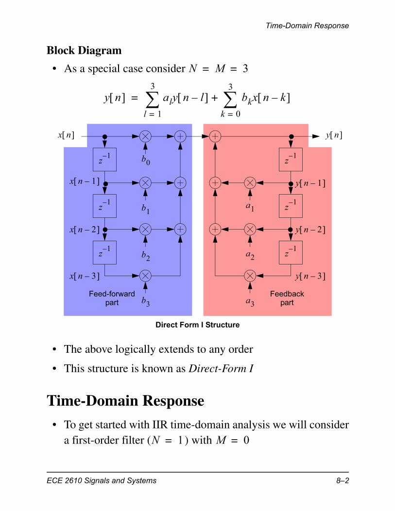
Block Diagram

• As a special case consider

• The above logically extends to any order

• This structure is known as Direct-Form I


• To get started with IIR time-domain analysis we will considera first-order filter ( ) with

N M 3= =

y n aly n l– l 1=

3

bkx n k– k 0=

3

+=

y n x n

z1–

z1–

z1–

z1–

z1–

z1–

y n 1–

y n 2–

y n 3–

x n 1–

x n 2–

x n 3–

b0

b1

b2

b3

a1

a2

a3Feed-forward

partFeedback

part

Direct Form I Structure

N 1= M 0=

ECE 2610 Signals and Systems 8–2


(8.3)

Impulse Response of a First-Order IIR System

• The impulse response can be obtained by setting and insuring that the system is initially at rest

• Definition: Initial rest conditions for an IIR filter means that:

– (1) The input is zero prior to the start time , that is for

– (2) The output is zero prior to the start time, that is for

• We now proceed to find the impulse response of (8.3) viadirect recursion of the difference equation

• In summary we have shown that the impulse response of a1st-order IIR filter is

(8.4)

where the unit step has been utilized to make it clearthat the output is zero for

y n a1y n 1– b0x n +=

x n n =

n0x n 0= n n0

y n 0= n n0

y 0 a1y 1– b0 0 + b0= =

y 1 a1y 0 b0 1 + a1b0= =

y 2 a1y 1 b0 2 + a12b0= =

y n a1nb0 n 0=

0

0

0

h n b0 a1 nu n =

u n n 0



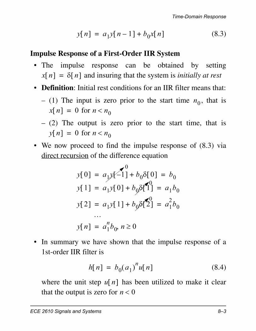
Example: First-Order IIR with

• The impulse response is

Linearity and Time Invariance of IIR Filters

• Recall that in Chapter 5 the definitions of time invariance andlinearity were introduced and shown to hold for FIR filters

• It can be shown that the general IIR difference equation alsoexhibits linearity and time invariance

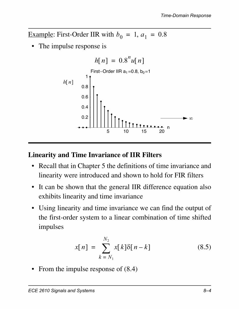
• Using linearity and time invariance we can find the output ofthe first-order system to a linear combination of time shiftedimpulses

(8.5)

• From the impulse response of (8.4)

b0 1 a1 0.8= =

h n 0.8nu n =

5 10 15 20n

0.2

0.4

0.6

0.8

1First�Order IIR a1�0.8, b0�1

h n

x n x k n k– k N1=

N2

=



(8.6)

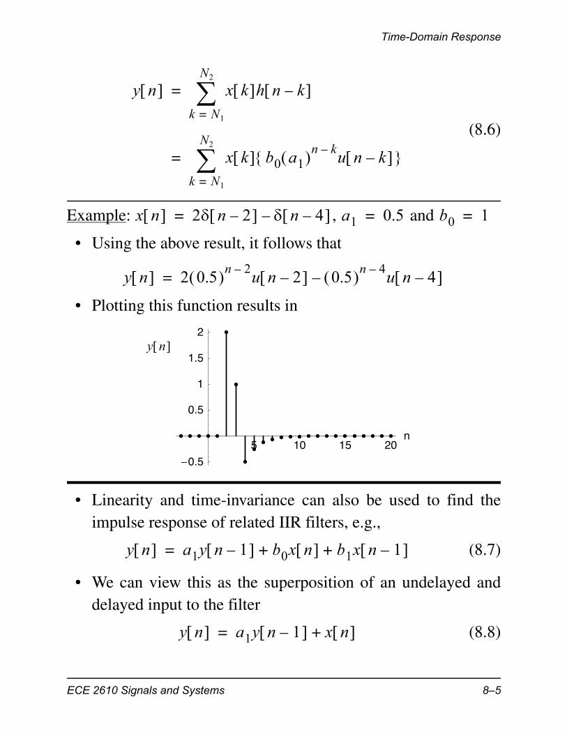
Example: , and

• Using the above result, it follows that

• Plotting this function results in

• Linearity and time-invariance can also be used to find theimpulse response of related IIR filters, e.g.,

(8.7)

• We can view this as the superposition of an undelayed anddelayed input to the filter

(8.8)

y n x k h n k– k N1=

N2

=

x k b0 a1 n k–u n k–

k N1=

N2

=

x n 2 n 2– n 4– –= a1 0.5= b0 1=

y n 2 0.5 n 2–u n 2– 0.5 n 4–

u n 4– –=

5 10 15 20n

�0.5

0.5

1

1.5

2y n

y n a1y n 1– b0x n b1x n 1– + +=

y n a1y n 1– x n +=



• Based on this observation, the impulse response is

(8.9)

Step Response of a First-Order Recursive System

• The step response allows us to see how a filter (system)responds to an infinitely long input

• We now consider the step response of

• Via direct recursion of the difference equation

• The summary form indicates a finite geometric series, whichhas solution

(8.10)

h n b0 a1 nu n b1 a1 n 1–u n 1– +=

b0 n b0 b1a11–

+ a1 nu n 1– +=

y n a1y n 1– b0x n +=

y 0 a1y 1– b0u 0 + b0= =

y 1 a1y 0 b0u 1 + a1b0 b0+= =

y 2 a1y 1 b0u 2 + a1 a1b0 b0+ b0+= =

y n b0 1 a1 a1

n+ + + b0 a1

k

k 0=

n

= =

0

rk

k 0=

L

1 r

L 1+–1 r–

--------------------- , r 1

L 1,+ r = 1

=



• Using (8.10) and assuming that , the step response ofthe first-order filter is

(8.11)

• Three conditions for exist

1. When the term grows without bound as n

becomes large, resulting in an unstable condition

2. When the term decays to zero as ,

and we have a stable condition3. When we have the special case output of (8.10)

where the output is of the form , which also

grows without bound; with the output alternates

sign, hence we have a marginally stable condition

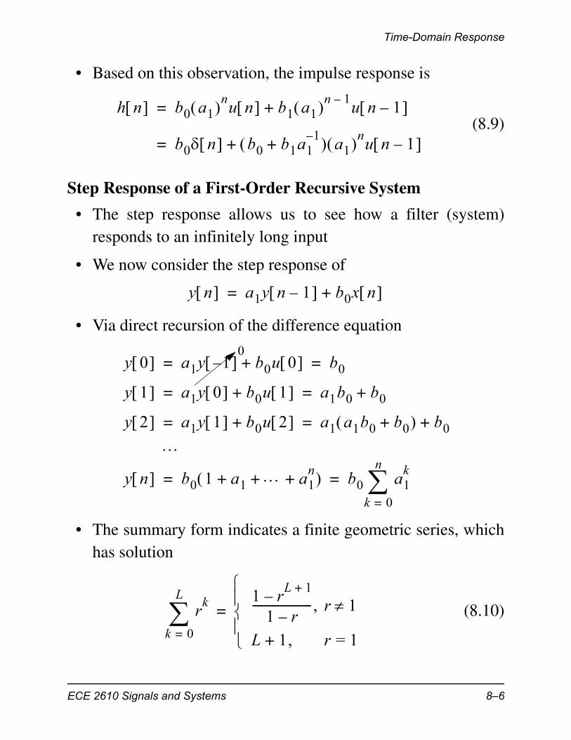
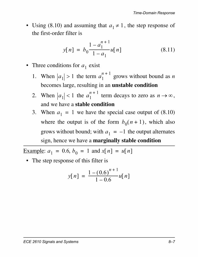
Example: and

• The step response of this filter is

a1 1

y n b0

1 a1n 1+

–

1 a1–---------------------u n =

a1

a1 1 a1n 1+

a1 1 a1n 1+

n

a1 1=

b0 n 1+

a1 1–=

a1 0.6 b0 1= = x n u n =

y n 1 0.6 n 1+–1 0.6–

-------------------------------u n =



• The step response can also be obtained by direct evaluationof the convolution sum

(8.4)

• For the problem at hand

(8.5)

• To evaluate this requires careful attention to details

• The product tells us how to set the sum limits

5 10 15 20n

0.5

1

1.5

2

2.5y n

y n x n *h n u n *h n = =

y n u k b0 a1 n k–u n k–

k –=

=

u k u n k–

k

k

n 0

0

0

u n k–

u k

n 0

n n


System Function of an IIR Filter

• The result is

(8.6)

which is the same result obtained by the direct recursion


• From our study of the z-transform we know that convolutionin the time (sequence)-domain corresponds to multiplicationin the z-domain

• For the case of IIR filters will be a fully rational func-tion, meaning in general both poles and zeros (more than at

)

• Begin by z-transforming both sides of the general IIR differ-ence equation using the delay property

y n b0 a1 n k–

k 0=

n

u n =

b0 a1 n a1 k–

k 0=

n

=

b0 a1 n1 1 a1 n 1+

–

1 1 a1 –------------------------------------=

b0

1 a1 n 1+–

1 a1 –-----------------------------=

y n x n *h n = X z H z Y z =z

H z

z 0=



(8.7)

• Form the ratio

(8.8)

• The coefficients of the numerator polynomial, denoted ,correspond to the feed-forward terms of the difference equa-tion

• The coefficients of the denominator polynomial, denoted, for correspond to the feedback terms of the

difference equation

• We have used various MATLAB functions that take as input band a coefficient vectors, e.g., filter(b,a,...),freqz(b,a,...), and zplane(b,a)

• In terms of the general IIR system we now identify those vec-tors as

(8.9)

Y z alzl–Y z

l 1=

N

bk zk–X z

k 0=

M

+=

ZT y n l– ZT x n k–

Y z X z H z =

H z

bkzk–

k 0=

M

1 alzl–

l 1=

N

–

------------------------------b0 b1z

1– bMzM–

+ + +

1 a1z1–

– aNzN–

––------------------------------------------------------------= =

B z

A z zl–l 0

b b0 b1 bM =

a 1 a1 a2– aN– – =



The General First-Order Case

• As a special case consider , then

(8.10)

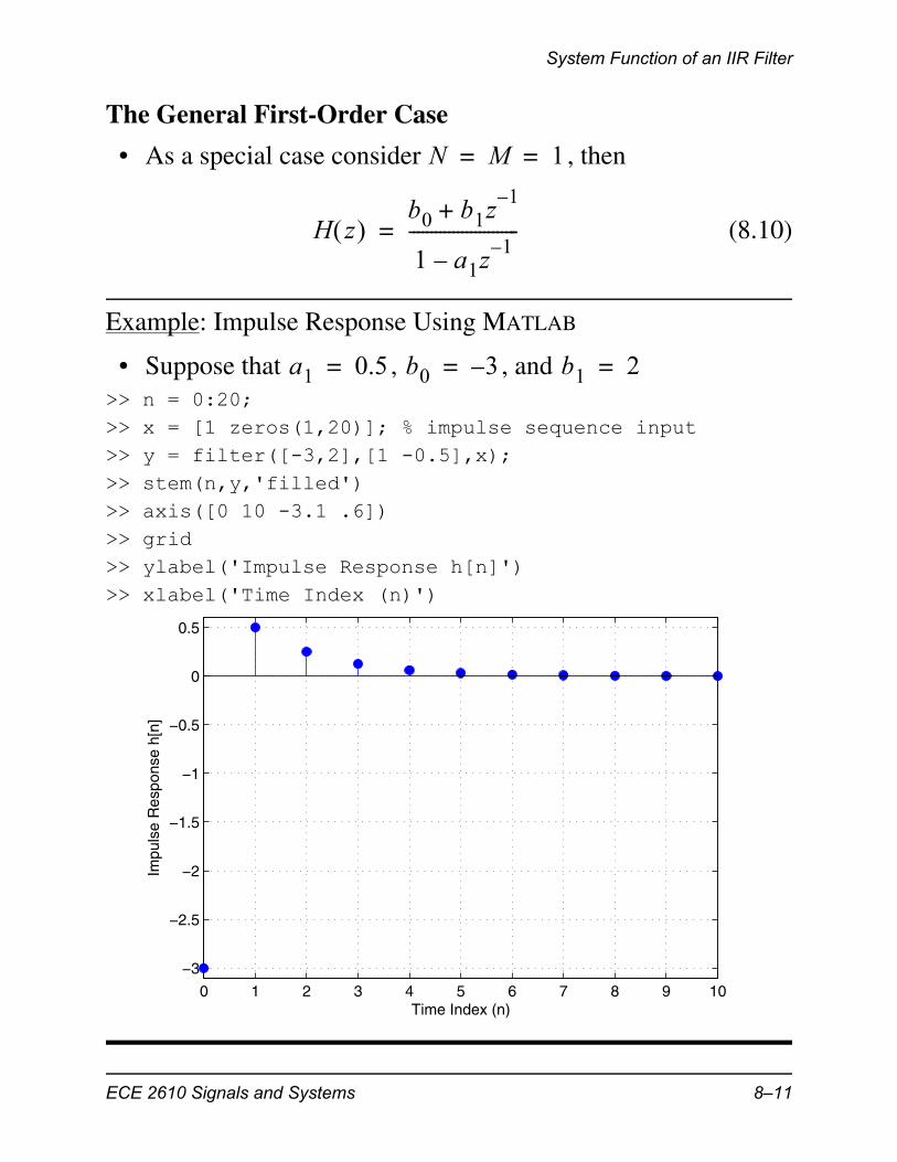
Example: Impulse Response Using MATLAB

• Suppose that , , and >> n = 0:20;>> x = [1 zeros(1,20)]; % impulse sequence input>> y = filter([-3,2],[1 -0.5],x);>> stem(n,y,'filled')>> axis([0 10 -3.1 .6])>> grid>> ylabel('Impulse Response h[n]')>> xlabel('Time Index (n)')

N M 1= =

H z b0 b1z

1–+

1 a1z1–

–-------------------------=

a1 0.5= b0 3–= b1 2=

0 1 2 3 4 5 6 7 8 9 10

−3

−2.5

−2

−1.5

−1

−0.5

0

0.5

Impu

lse

Res

pons

e h[

n]

Time Index (n)



Example: y = filter([1 1],[1 -0.8],x)

• We wish to find the system function, impulse response, anddifference equation that corresponds to the given filter()expression

• By inspection

• The impulse response using page 8–5, eqns (8.7)—(8.9)

• The difference equation is

System Functions and Block-Diagram Structures

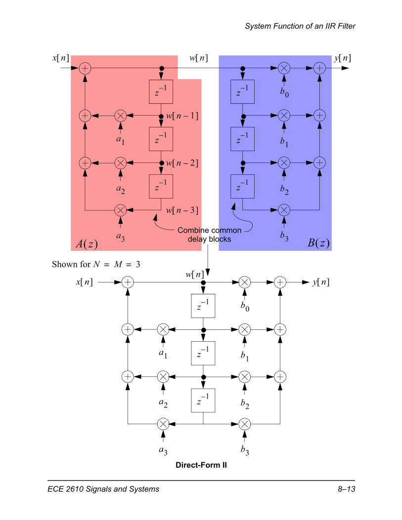
• We have already examined the Direct-Form I structure (p. 8–2)

• The Direct-Form I structure implements the feed-forwardterms first followed by the feedback terms

• We can view this as a cascade of two systems, which due tolinearity can also be written as

(8.11)

• In the block diagram this is represented as

H z 1 z1–

+

1 0.8z1–

–------------------------=

h n n 1 0.81–

+ 0.8 nu n 1– +=

y n 0.8y n 1– x n x n 1– + +=

H z B z 1A z ----------- 1

A z ----------- B z = =



y n x n

z1–

z1–

z1–

z1–

z1–

z1–

w n 1–

w n 2–

w n 3–

b0

b1

b2

b3

a1

a2

a3

w n

Combine commondelay blocks

z1–

z1–

z1–

b0

b1

b2

b3

a1

a2

a3

x n y n

Direct-Form II

w n

A z B z

Shown for N M 3= =



• The Direct-Form II structure uses fewer delay blocks thanDirect-Form I

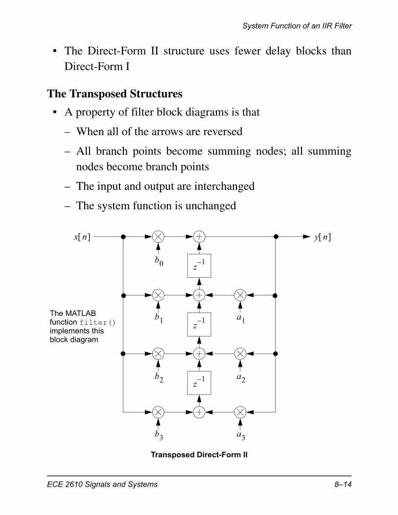
The Transposed Structures

• A property of filter block diagrams is that

– When all of the arrows are reversed

– All branch points become summing nodes; all summingnodes become branch points

– The input and output are interchanged

– The system function is unchanged

b1

b2

b3

z1–

z1–

z1–

a1

a2

a3

b0

x n y n

Transposed Direct-Form II

The MATLABfunction filter()implements thisblock diagram



Relation to the Impulse Response

• From Chapter 7 we know that the impulse response and sys-tem function are related via the z-transform

• For IIR systems more work is required to obtain the z-trans-form

• Consider , where we have learnedthat the impulse response is

• From the definition of the z-transform,

(8.12)

• The sum of (8.12) is an infinite geometric series which ingeneral terms is

• Applying the sum formula to (8.12) results in

(8.13)

– The condition that tells us that the z-transformonly exists for these values of z

– The z-plane region is known as the region of convergence

• We have thus established the following z-transform relation-

y n ay n 1– x n +=

h n anu n =

H z anzn–

n 0=

az1– n

n 0=

= =

S rn

n 0=

11 r–----------- r 1= =

H z az1– n

n 0=

1

1 az1–

–------------------- z a= =

z a


Poles and Zeros

ship

(8.14)

• We can use this result to find the z-transform of

(8.15)

directly using just linearity and the delay property

• We will learn later that we can work this operation in reverse,and when combined with partial fraction expansion, we willbe able to find the inverse z-transform of almost any rational

Poles and Zeros

• Factoring the numerator denominator polynomials allows usto discover the poles and zeros of

• For the case of a first-order system only algebra is needed

anu n 1

1 az1–

–-------------------

z

h n b0 a1 nu n b1 a1 n 1–u n 1– +=

H z b01

1 a1z1–

–---------------------- b1z

1– 1

1 a1z1–

–----------------------+=

b0 b1z1–

+

1 a1z1–

–-------------------------=

H z

H z

H z b0 b1z

1–+

1 a1z1–

–------------------------- z

z--

b0z b1+

z a1–-------------------- b0

z b1 b0+

z a1–-----------------------= = =


Poles and Zeros

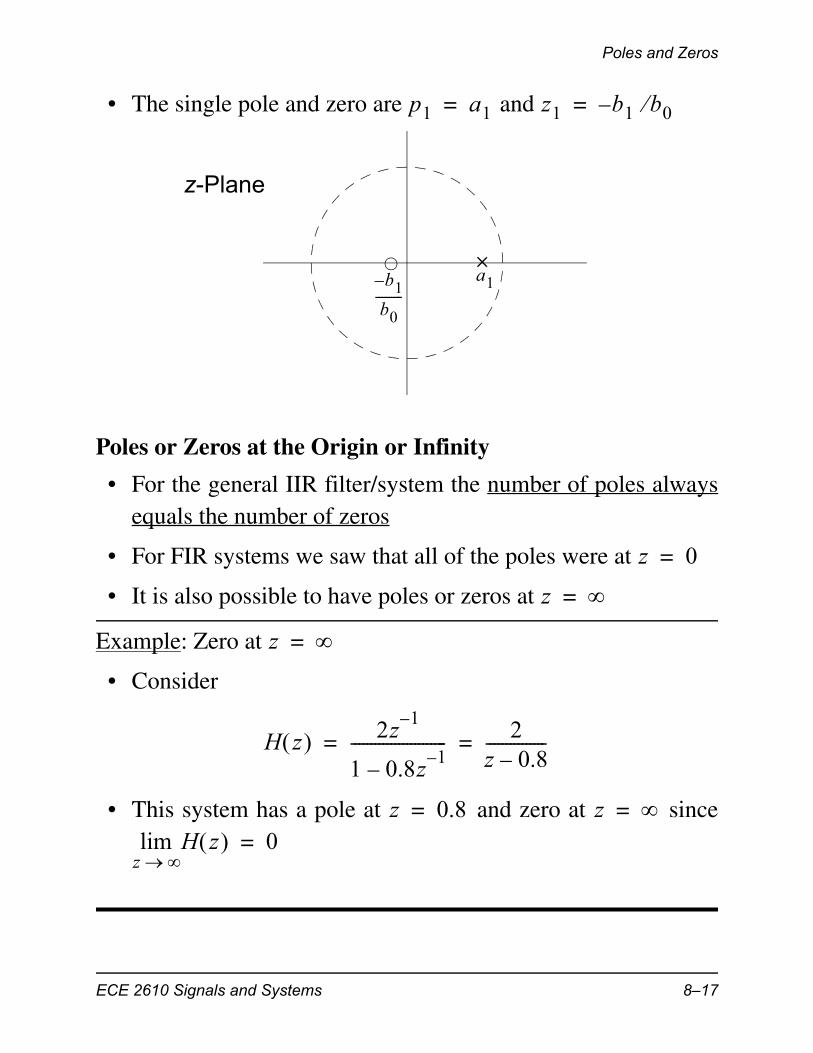
• The single pole and zero are and

Poles or Zeros at the Origin or Infinity

• For the general IIR filter/system the number of poles alwaysequals the number of zeros

• For FIR systems we saw that all of the poles were at

• It is also possible to have poles or zeros at

Example: Zero at

• Consider

• This system has a pole at and zero at since

p1 a1= z1 b1 b0–=

a1b1–

b0---------

z-Plane

z 0=

z =

z =

H z 2z1–

1 0.8z1–

–------------------------ 2

z 0.8–---------------= =

z 0.8= z =H z

z lim 0=


Poles and Zeros

Example: Pole at

• Consider

• This system has a pole at and a zero at

Pole Locations and Stability

• We know that

(8.16)

• We note that this system has a pole at and a zero at

• The impulse response decays to zero so long as ,which is equivalent to requiring that the pole lies inside theunit circle

• System Stability: Causal LTI IIR systems, initially at rest,are stable if all of the poles of the system function lie insidethe unit circle

Example:

• Converting to positive powers of z

z =

H z 1 0.5z1–

+

z1–

------------------------ z 0.5+= =

z = z 0.5–=

h n anu n =

1

1 az1–

–------------------- H z =

z

z a=z 0=

a 1

H z 1 5z1–

– 1 0.995z1–

– =

H z z 5–z 0.995–---------------------= Pole at z 0.995 so stable=


Poles and Zeros

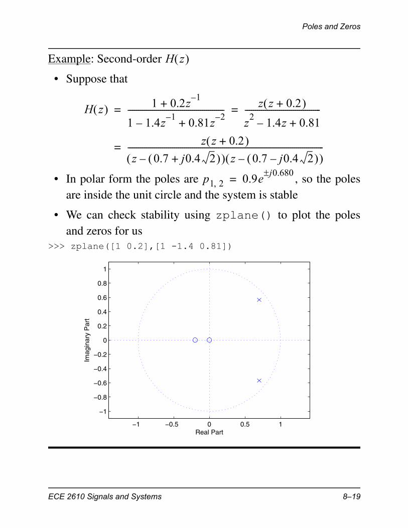
Example: Second-order

• Suppose that

• In polar form the poles are , so the polesare inside the unit circle and the system is stable

• We can check stability using zplane() to plot the polesand zeros for us

>>> zplane([1 0.2],[1 -1.4 0.81])

H z

H z 1 0.2z1–

+

1 1.4z1–

– 0.81z2–

+------------------------------------------------ z z 0.2+

z2

1.4z– 0.81+--------------------------------------= =

z z 0.2+ z 0.7 j0.4 2+ – z 0.7 j0.4 2– –

--------------------------------------------------------------------------------------------------=

p1 2 0.9ej0.680

=

−1 −0.5 0 0.5 1

−1

−0.8

−0.6

−0.4

−0.2

0

0.2

0.4

0.6

0.8

1

Real Part

Imag

inar

y P

art


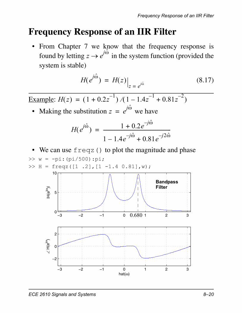
Frequency Response of an IIR Filter


• From Chapter 7 we know that the frequency response isfound by letting in the system function (provided thesystem is stable)

(8.17)

Example:

• Making the substitution we have

• We can use freqz() to plot the magnitude and phase>> w = -pi:(pi/500):pi;>> H = freqz([1 .2],[1 -1.4 0.81],w);

z ej

H ej H z

z ej==

H z 1 0.2z1–

+ 1 1.4z1–

– 0.81z2–

+ =

z ej

=

H ej 1 0.2e

j– +

1 1.4ej–

– 0.81ej– 2

+---------------------------------------------------------=

−3 −2 −1 0 1 2 30

5

10

|H(e

jω)|

−3 −2 −1 0 1 2 3

−2

0

2

∠ H

(ejω

)

hat(ω)

0.680

BandpassFilter



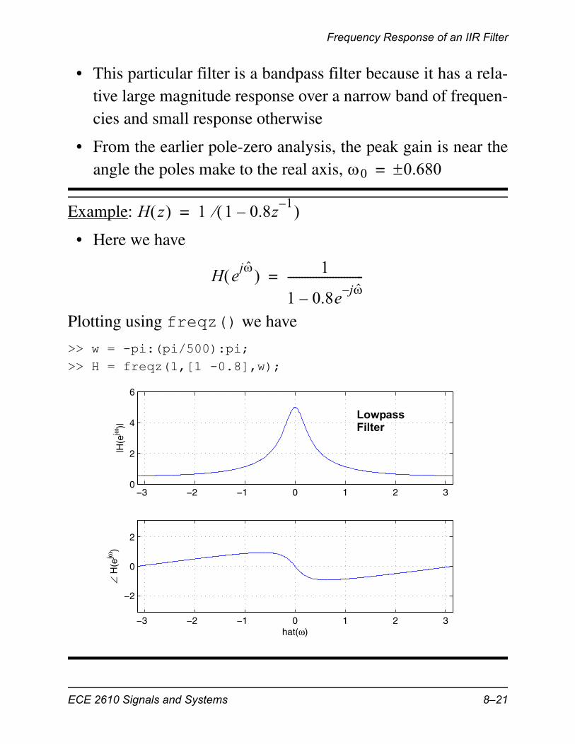
• This particular filter is a bandpass filter because it has a rela-tive large magnitude response over a narrow band of frequen-cies and small response otherwise

• From the earlier pole-zero analysis, the peak gain is near theangle the poles make to the real axis,

Example:

• Here we have

Plotting using freqz() we have

>> w = -pi:(pi/500):pi;>> H = freqz(1,[1 -0.8],w);

0 0.680=

H z 1 1 0.8z1–

– =

H ej 1

1 0.8ej–

–---------------------------=

−3 −2 −1 0 1 2 30

2

4

6

|H(e

jω)|

−3 −2 −1 0 1 2 3

−2

0

2

∠ H

(ejω

)

hat(ω)

LowpassFilter



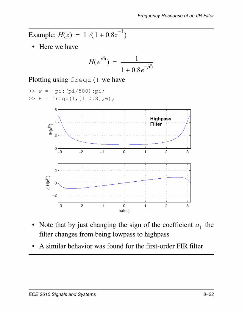
Example:

• Here we have

Plotting using freqz() we have

>> w = -pi:(pi/500):pi;>> H = freqz(1,[1 0.8],w);

• Note that by just changing the sign of the coefficient thefilter changes from being lowpass to highpass

• A similar behavior was found for the first-order FIR filter

H z 1 1 0.8z1–

+ =

H ej 1

1 0.8ej–

+---------------------------=

−3 −2 −1 0 1 2 30

2

4

6

|H(e

jω)|

−3 −2 −1 0 1 2 3

−2

0

2

∠ H

(ejω

)

hat(ω)

HighpassFilter

a1


The Inverse z-Transform and Applications

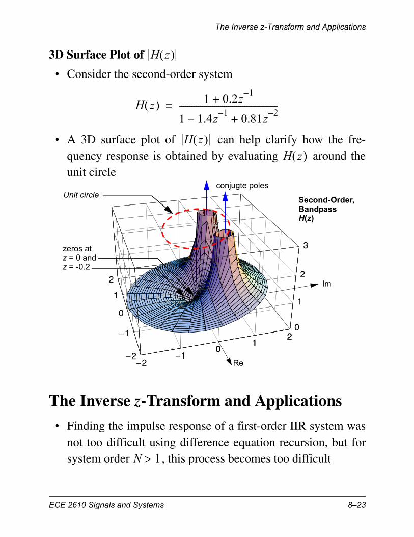
3D Surface Plot of

• Consider the second-order system

• A 3D surface plot of can help clarify how the fre-quency response is obtained by evaluating around theunit circle


• Finding the impulse response of a first-order IIR system wasnot too difficult using difference equation recursion, but forsystem order , this process becomes too difficult

H z

H z 1 0.2z1–

+

1 1.4z1–

– 0.81z2–

+------------------------------------------------=

H z H z

�2�1

01

2

�2

�1

0

1

2

0

1

2

3

10

12

Re

Im

conjugte poles

zeros atz = 0 andz = -0.2

Unit circleSecond-Order,BandpassH(z)

N 1



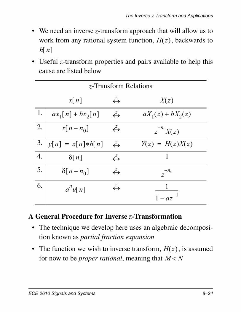
• We need an inverse z-transform approach that will allow us towork from any rational system function, , backwards to

• Useful z-transform properties and pairs available to help thiscause are listed below

A General Procedure for Inverse z-Transformation

• The technique we develop here uses an algebraic decomposi-tion known as partial fraction expansion

• The function we wish to inverse transform, , is assumedfor now to be proper rational, meaning that

z-Transform Relations

1.

2.

3.

4. 1

5.

6.

H z h n

x n z X z

ax1 n bx2 n + z aX1 z bX2 z +

x n n0– z zn0–X z

y n x n *h n = z Y z H z X z =

n z

n n0– z zn0–

anu n z 1

1 az1–

–-------------------

H z M N



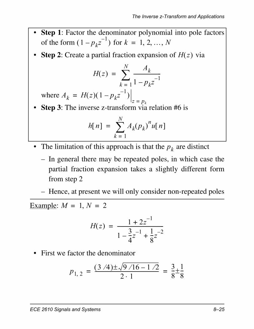
• Step 1: Factor the denominator polynomial into pole factorsof the form for

• Step 2: Create a partial fraction expansion of via

where

• Step 3: The inverse z-transform via relation #6 is

• The limitation of this approach is that the are distinct

– In general there may be repeated poles, in which case thepartial fraction expansion takes a slightly different formfrom step 2

– Hence, at present we will only consider non-repeated poles

Example:

• First we factor the denominator

1 pkz1–

– k 1 2 N =

H z

H z Ak

1 pkz1–

–----------------------

k 1=

N

=

Ak H z 1 pkz1–

– z pk=

=

h n Ak pk nu n k 1=

N

=

pk

M 1 N 2= =

H z 1 2z1–

+

134---z

1––

18---z

2–+

-------------------------------------=

p1 23 4 9 16 1 2–

2 1---------------------------------------------------

38--- 1

8---= =



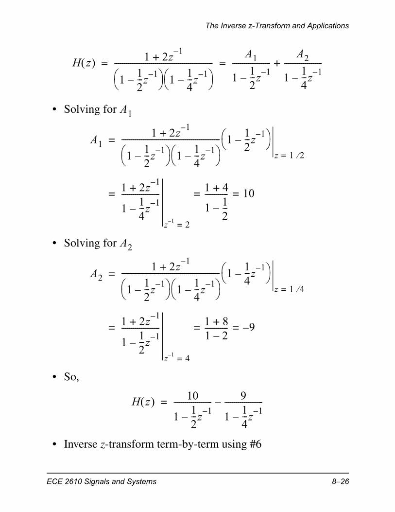
• Solving for

• Solving for

• So,

• Inverse z-transform term-by-term using #6

H z 1 2z1–

+

112---z

1––

114---z

1––

---------------------------------------------------

A1

112---z

1––

--------------------A2

114---z

1––

--------------------+= =

A1

A11 2z

1–+

112---z

1––

114---z

1––

--------------------------------------------------- 1

12---z

1––

z 1 2=

=

1 2z1–

+

114---z

1––

--------------------

z 1– 2=

1 4+

1 12---–

------------ 10= ==

A2

A21 2z

1–+

112---z

1––

114---z

1––

--------------------------------------------------- 1

14---z

1––

z 1 4=

=

1 2z1–

+

112---z

1––

--------------------

z 1– 4=

1 8+1 2–------------ 9–= ==

H z 10

112---z

1––

-------------------- 9

114---z

1––

--------------------–=



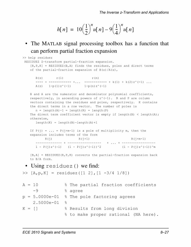
• The MATLAB signal processing toolbox has a function thatcan perform partial fraction expansion

>> help residuez RESIDUEZ Z-transform partial-fraction expansion. [R,P,K] = RESIDUEZ(B,A) finds the residues, poles and direct terms of the partial-fraction expansion of B(z)/A(z), B(z) r(1) r(n) ---- = ------------ +... ------------ + k(1) + k(2)z^(-1) ... A(z) 1-p(1)z^(-1) 1-p(n)z^(-1) B and A are the numerator and denominator polynomial coefficients, respectively, in ascending powers of z^(-1). R and P are column vectors containing the residues and poles, respectively. K contains the direct terms in a row vector. The number of poles is n = length(A)-1 = length(R) = length(P) The direct term coefficient vector is empty if length(B) < length(A); otherwise, length(K) = length(B)-length(A)+1 If P(j) = ... = P(j+m-1) is a pole of multiplicity m, then the expansion includes terms of the form R(j) R(j+1) R(j+m-1) -------------- + ------------------ + ... + ------------------ 1 - P(j)z^(-1) (1 - P(j)z^(-1))^2 (1 - P(j)z^(-1))^m [B,A] = RESIDUEZ(R,P,K) converts the partial-fraction expansion back to B/A form.

• Using residuez() we find:>> [A,p,K] = residuez([1 2],[1 -3/4 1/8])

A = 10 % The partial fraction coefficients -9 % agreep = 5.0000e-01 % The pole factoring agrees 2.5000e-01 % K = [] % Results from long division % to make proper rational (NA here).

h n 1012--- nu n 9

14--- nu n –=



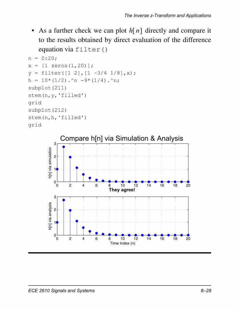
• As a further check we can plot directly and compare itto the results obtained by direct evaluation of the differenceequation via filter()

n = 0:20;x = [1 zeros(1,20)];y = filter([1 2],[1 -3/4 1/8],x);h = 10*(1/2).^n -9*(1/4).^n;subplot(211)stem(n,y,'filled')gridsubplot(212)stem(n,h,'filled')grid

h n

0 2 4 6 8 10 12 14 16 18 200

1

2

3

h[n]

via

sim

ulat

ion

0 2 4 6 8 10 12 14 16 18 200

1

2

3

h[n]

via

ana

lysi

s

Time Index (n)

Compare h[n] via Simulation & Analysis

They agree!



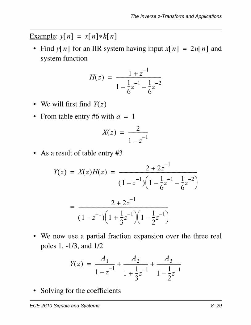
Example:

• Find for an IIR system having input andsystem function

• We will first find

• From table entry #6 with

• As a result of table entry #3

• We now use a partial fraction expansion over the three realpoles 1, -1/3, and 1/2

• Solving for the coefficients

y n x n *h n =

y n x n 2u n =

H z 1 z1–

+

116---z

1––

16---z

2––

-------------------------------------=

Y z

a 1=

X z 2

1 z1–

–----------------=

Y z X z H z 2 2z1–

+

1 z1–

– 116---z

1––

16---z

2––

----------------------------------------------------------------= =

2 2z1–

+

1 z1–

– 113---z

1–+

112---z

1––

-------------------------------------------------------------------------=

Y z A1

1 z1–

–----------------

A2

113---z

1–+

--------------------A3

112---z

1––

--------------------+ +=



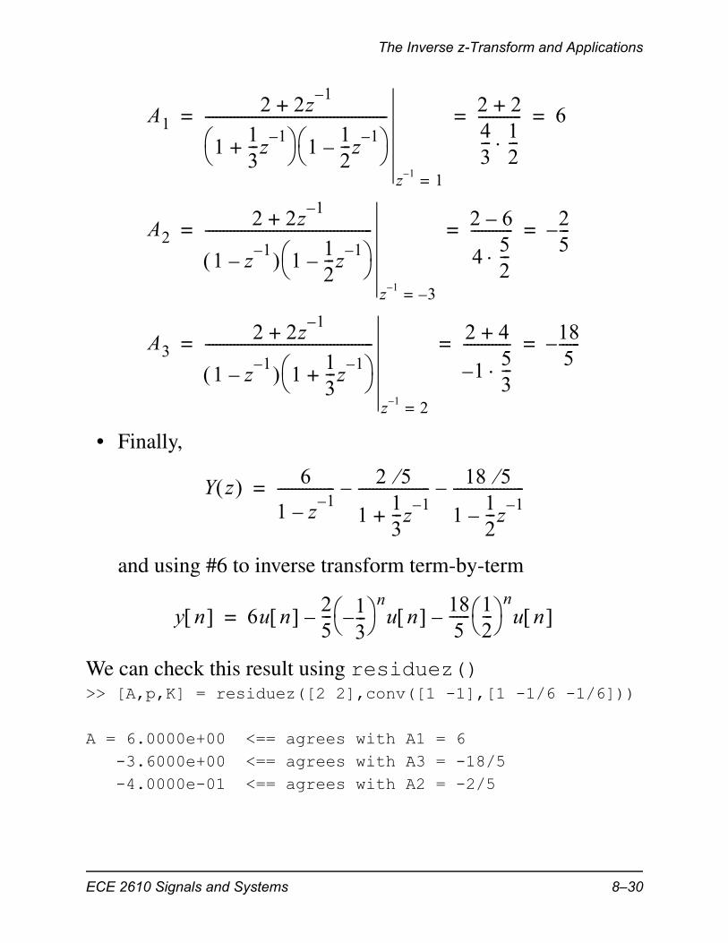
• Finally,

and using #6 to inverse transform term-by-term

We can check this result using residuez()>> [A,p,K] = residuez([2 2],conv([1 -1],[1 -1/6 -1/6]))

A = 6.0000e+00 <== agrees with A1 = 6 -3.6000e+00 <== agrees with A3 = -18/5 -4.0000e-01 <== agrees with A2 = -2/5

A12 2z

1–+

113---z

1–+

112---z

1––

---------------------------------------------------

z 1– 1=

2 2+43--- 1

2---

------------ 6= = =

A22 2z

1–+

1 z1–

– 112---z

1––

-----------------------------------------------

z 1– 3–=

2 6–

452---

------------ 25---–= = =

A32 2z

1–+

1 z1–

– 113---z

1–+

-----------------------------------------------

z 1– 2=

2 4+

1–53---

------------- 185------–= = =

Y z 6

1 z1–

–---------------- 2 5

113---z

1–+

--------------------– 18 5

112---z

1––

--------------------–=

y n 6u n 25--- 1

3---–

nu n –185------ 1

2--- nu n –=



p = 1.0000e+00 5.0000e-01 -3.3333e-01

K = []

• The results agree!

• The partial fraction expansion technique requires that

• If the rational function does not satisfy this condition we canperform long division to reduce the order of the denominatorto the point where

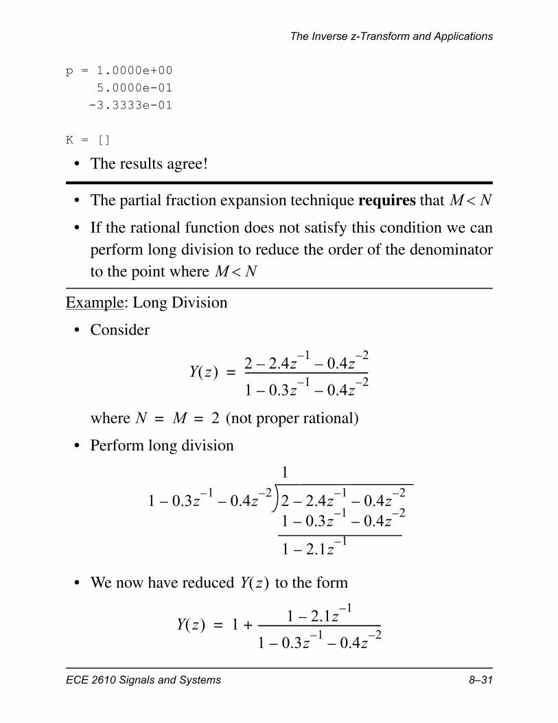
Example: Long Division

• Consider

where (not proper rational)

• Perform long division

• We now have reduced to the form

M N

M N

Y z 2 2.4z1–

– 0.4z2–

–

1 0.3z1–

– 0.4z2–

–---------------------------------------------=

N M 2= =

1 0.3z1–

– 0.4z2–

– 2 2.4z1–

– 0.4z2–

–

1

1 0.3z1–

– 0.4z2–

–

1 2.1z1–

–

Y z

Y z 1 1 2.1z1–

–

1 0.3z1–

– 0.4z2–

–---------------------------------------------+=



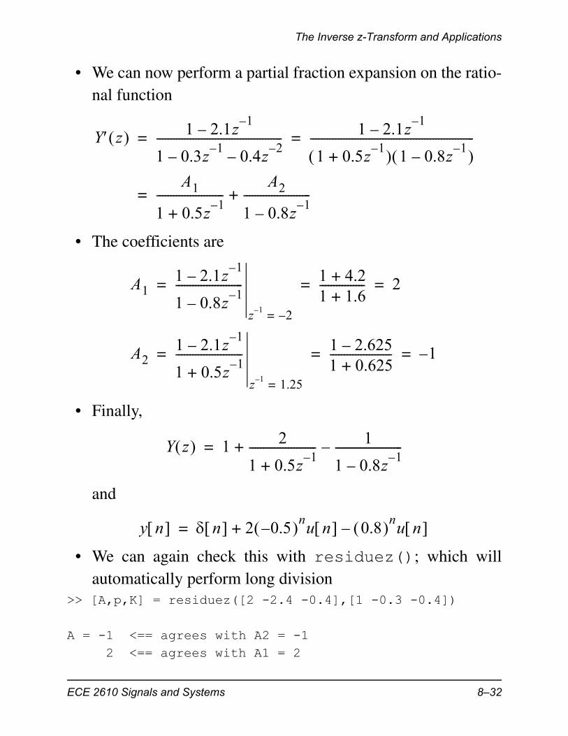
• We can now perform a partial fraction expansion on the ratio-nal function

• The coefficients are

• Finally,

and

• We can again check this with residuez(); which willautomatically perform long division

>> [A,p,K] = residuez([2 -2.4 -0.4],[1 -0.3 -0.4])

A = -1 <== agrees with A2 = -1 2 <== agrees with A1 = 2

Y z 1 2.1z1–

–

1 0.3z1–

– 0.4z2–

–--------------------------------------------- 1 2.1z

1––

1 0.5z1–

+ 1 0.8z1–

– -----------------------------------------------------------= =

A1

1 0.5z1–

+------------------------

A2

1 0.8z1–

–------------------------+=

A11 2.1z

1––

1 0.8z1–

–------------------------

z 1– 2–=

1 4.2+1 1.6+---------------- 2= = =

A21 2.1z

1––

1 0.5z1–

+------------------------

z 1– 1.25=

1 2.625–1 0.625+---------------------- 1–= = =

Y z 1 2

1 0.5z1–

+------------------------ 1

1 0.8z1–

–------------------------–+=

y n n 2 0.5– nu n 0.8 nu n –+=


Steady-State Response and Stability

p = 8.0000e-01 -5.0000e-01

K = 1 <== Long division term

• The value is the result of long division (see the helpfor residuez())

• The answers agree!


• The sinusoidal steady-state response developed in Chapter 6for FIR filters also holds for IIR filters

• It can be shown (see Text Section 8-8 for more details, espe-cially for ) that for

(8.18)

and an IIR system with , the system output willbe

(8.19)

where are the poles of and the arethe corresponding partial fraction coefficients

• The first term represents the transient response, which pro-vided all the poles of lie inside the unit circle, willdecay to zero, leaving just the sinusoidal term

K 1=

N 1=

x n ej0nu n =

H z N M

y n Ak pk nu n k 1=

N

H ej0 ej0nu n +=

pk k 1 N = H z Ak

H z



• For the output to reach sinusoidal steady-state we must have to insure that the transient term (first term) decays to

zero, this then insures that the system is stable

• Summary: Poles inside the unit circle to insure stability

Example:

• Input a cosine with starting at to the sys-tem

• This is a second-order IIR filter, so the transient term consistsof two exponentials

• Second-order system will be studied in more detail in thenext section

• Observe the transient using MATLAB

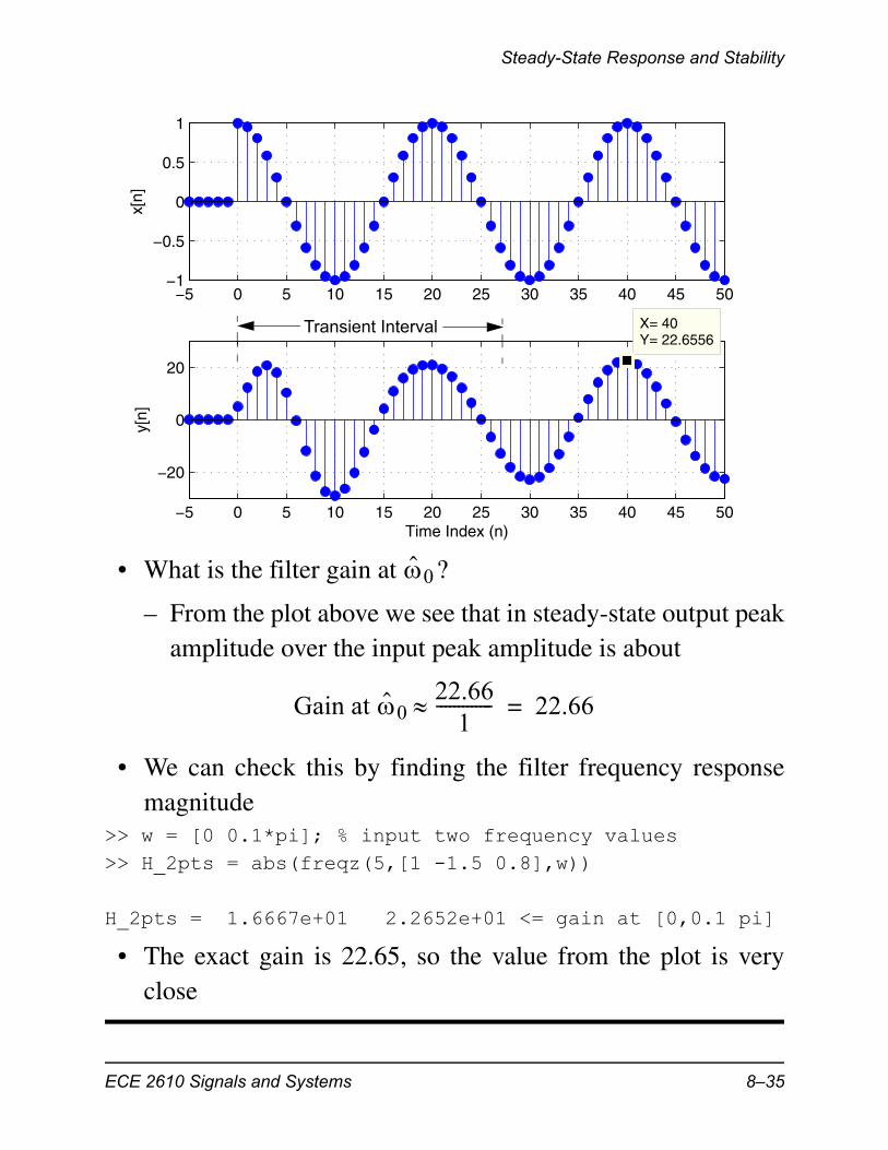
>> n = -5:50;>> x = cos(2*pi/20*n).*ustep(n,0);>> y = filter(5,[1 -1.5 0.8],x);>> subplot(211)>> stem(n,x,'filled')>> axis([-5 50 -1 1]); grid>> ylabel('x[n]')>> subplot(212)>> stem(n,y,'filled')>> axis([-5 50 -30 30]); grid>> ylabel('y[n]')>> xlabel('Time Index (n)')

pk 1

x n 2 20 n u n cos=

0 0.1= n 0=

H z 5

1 1.8z1–

– 0.9z2–

+---------------------------------------------=



• What is the filter gain at ?

– From the plot above we see that in steady-state output peakamplitude over the input peak amplitude is about

• We can check this by finding the filter frequency responsemagnitude

>> w = [0 0.1*pi]; % input two frequency values>> H_2pts = abs(freqz(5,[1 -1.5 0.8],w))

H_2pts = 1.6667e+01 2.2652e+01 <= gain at [0,0.1 pi]

• The exact gain is 22.65, so the value from the plot is veryclose

−5 0 5 10 15 20 25 30 35 40 45 50−1

−0.5

0

0.5

1x[

n]

−5 0 5 10 15 20 25 30 35 40 45 50

−20

0

20

X= 40Y= 22.6556

y[n]

Time Index (n)

Transient Interval

0

Gain at 022.66

1------------- 22.66=


Second-Order Filters


• Second-order IIR filters allow for the possibility of complexconjugate pole and zero pairs, yet still have real coefficients

• The general second-order system function is

(8.20)

• The corresponding difference equation is

(8.21)

• The direct-form I and direct-form II structures, discussed onpages 8–2 and 8–13 respectively, can be used to implement(8.21)

Poles and Zeros

• To identify the poles and zeros of we can first convertto positive powers of z and then factor into poles and zeros

• The coefficients are related to the roots (poles & zeros) via

(8.22)

H z b0 b1z

1–b2z

2–+ +

1 a1z1–

– a2z2–

–---------------------------------------------=

y n a1y n 1– a2y n 2– +=

b0x n b1x n 1– b2x n 2– + + +

H z

H z b0z

2b1z b2+ +

z2a1z– a2+

------------------------------------- b0

z z1– z z2– z p1– z p2–

-------------------------------------= =

b1 b0 z1 z2+ –= b2 b0 z1z2=

a1 p1 p2+= a2 p1p2–=



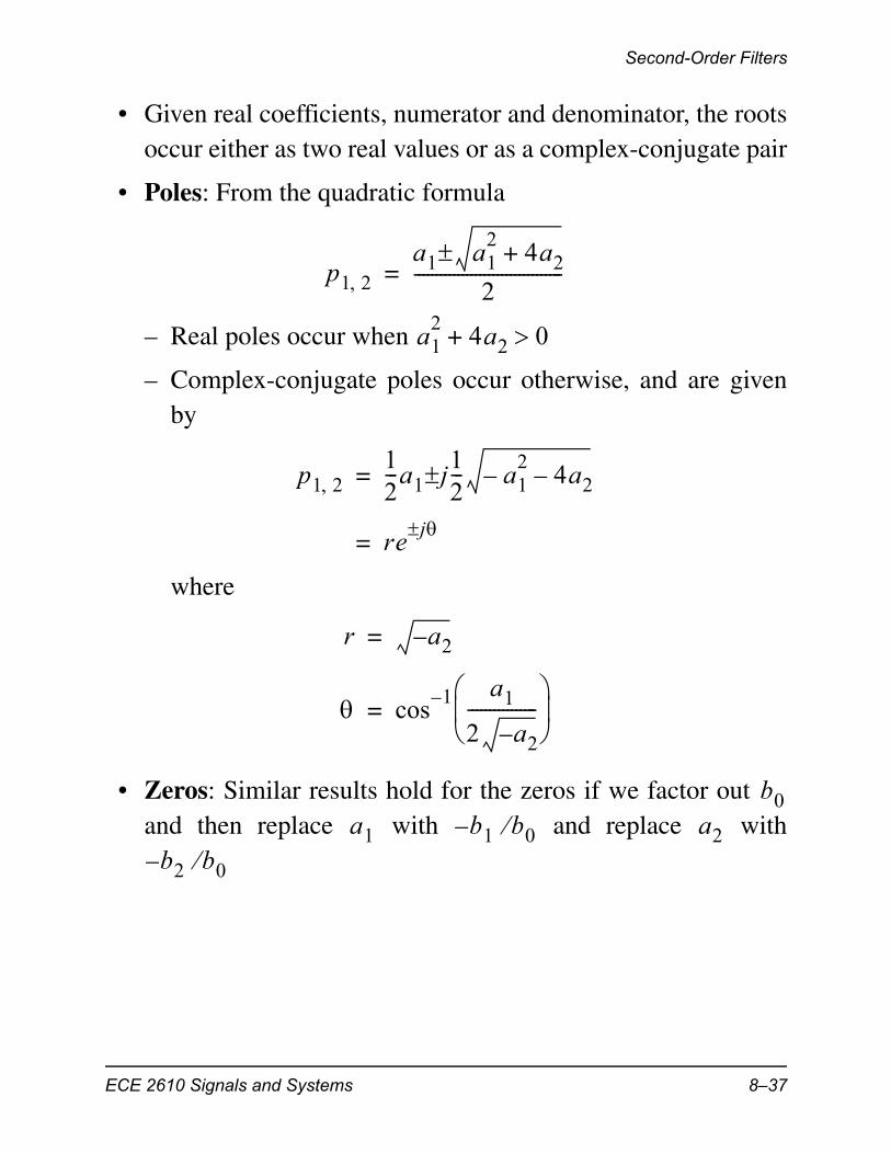
• Given real coefficients, numerator and denominator, the rootsoccur either as two real values or as a complex-conjugate pair

• Poles: From the quadratic formula

– Real poles occur when

– Complex-conjugate poles occur otherwise, and are givenby

where

• Zeros: Similar results hold for the zeros if we factor out and then replace with and replace with

p1 2a1 a1

24a2+

2----------------------------------=

a12

4a2+ 0

p1 212---a1 j

12--- a1

2– 4a2–=

rej

=

r a2–=

cos1– a1

2 a2–----------------

=

b0a1 b1 b0– a2

b2 b0–



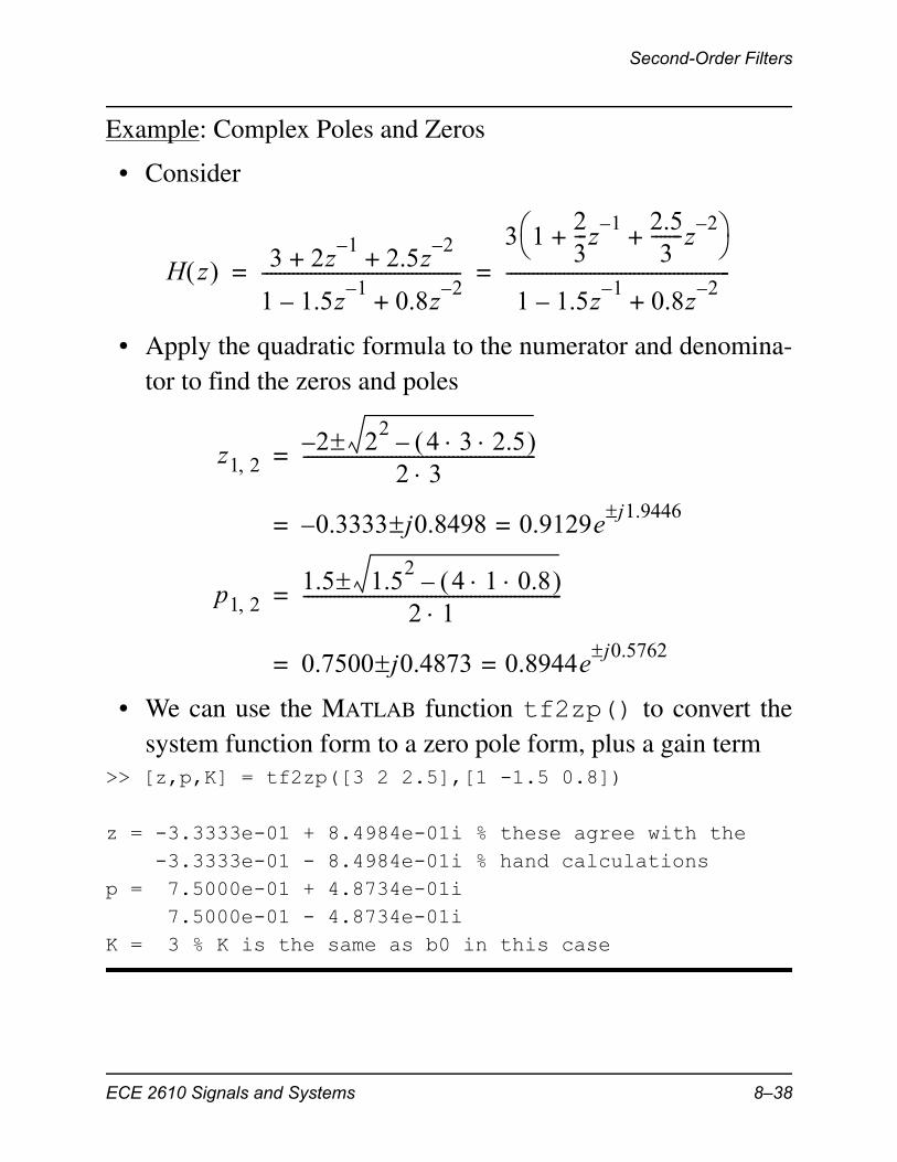
Example: Complex Poles and Zeros

• Consider

• Apply the quadratic formula to the numerator and denomina-tor to find the zeros and poles

• We can use the MATLAB function tf2zp() to convert thesystem function form to a zero pole form, plus a gain term

>> [z,p,K] = tf2zp([3 2 2.5],[1 -1.5 0.8])

z = -3.3333e-01 + 8.4984e-01i % these agree with the -3.3333e-01 - 8.4984e-01i % hand calculationsp = 7.5000e-01 + 4.8734e-01i 7.5000e-01 - 4.8734e-01iK = 3 % K is the same as b0 in this case

H z 3 2z1–

2.5z2–

+ +

1 1.5z1–

– 0.8z2–

+---------------------------------------------

3 123---z

1– 2.53

-------z2–

+ +

1 1.5z1–

– 0.8z2–

+---------------------------------------------------= =

z1 22 2

24 3 2.5 ––

2 3-----------------------------------------------------=

0.3333 j0.8498– 0.9129ej1.9446

==

p1 21.5 1.5

24 1 0.8 –

2 1-----------------------------------------------------------=

0.7500 j0.4873 0.8944ej0.5762

==



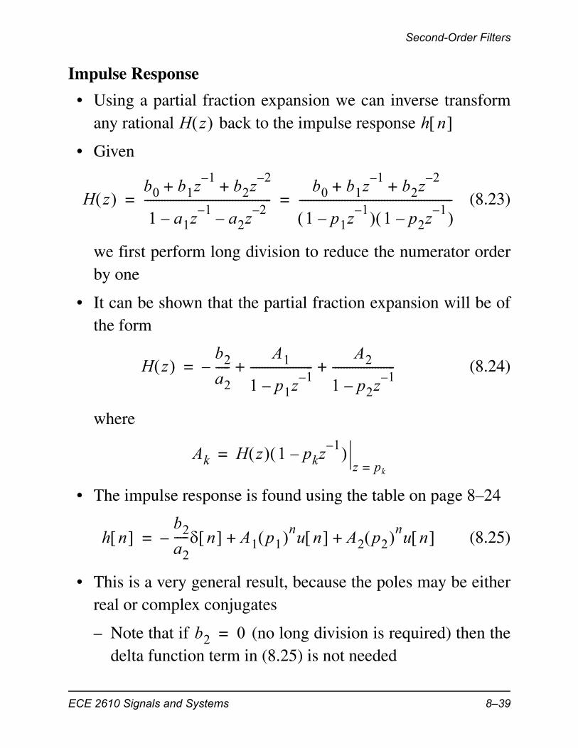
Impulse Response

• Using a partial fraction expansion we can inverse transformany rational back to the impulse response

• Given

(8.23)

we first perform long division to reduce the numerator orderby one

• It can be shown that the partial fraction expansion will be ofthe form

(8.24)

where

• The impulse response is found using the table on page 8–24

(8.25)

• This is a very general result, because the poles may be eitherreal or complex conjugates

– Note that if (no long division is required) then thedelta function term in (8.25) is not needed

H z h n

H z b0 b1z

1–b2z

2–+ +

1 a1z1–

– a2z2–

–---------------------------------------------

b0 b1z1–b2z

2–+ +

1 p1z1–

– 1 p2z1–

– ------------------------------------------------------= =

H z b2

a2-----–

A1

1 p1z1–

–----------------------

A2

1 p2z1–

–----------------------+ +=

Ak H z 1 pkz1–

– z pk=

=

h n b2

a2----- n – A1 p1 nu n A2 p2 nu n + +=

b2 0=



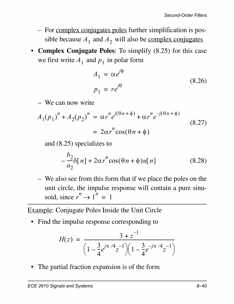
– For complex conjugates poles further simplification is pos-sible because and will also be complex conjugates

• Complex Conjugate Poles: To simplify (8.25) for this casewe first write and in polar form

(8.26)

– We can now write

(8.27)

and (8.25) specializes to

(8.28)

– We also see from this form that if we place the poles on theunit circle, the impulse response will contain a pure sinu-soid, since

Example: Conjugate Poles Inside the Unit Circle

• Find the impulse response corresponding to

• The partial fraction expansion is of the form

A1 A2

A1 p1

A1 ej=

p1 rej

=

A1 p1 n A2 p2 n+ rnej n + rne j n + –+=

2rn n + cos=

b2

a2----- n – 2rn n + u n cos+

rn

1n 1=

H z 3 z1–

+

134---ej 4

z1–

– 1

34---e

j– 4z

1––

-------------------------------------------------------------------------------=



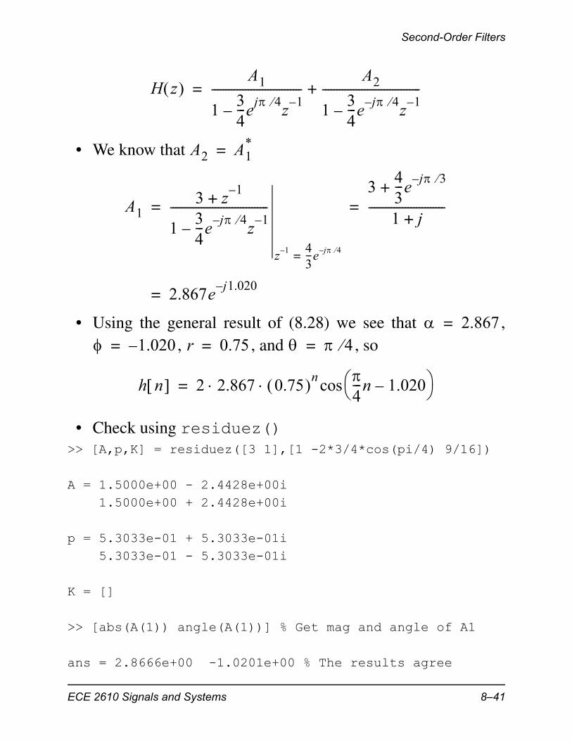
• We know that

• Using the general result of (8.28) we see that ,, , and , so

• Check using residuez()>> [A,p,K] = residuez([3 1],[1 -2*3/4*cos(pi/4) 9/16])

A = 1.5000e+00 - 2.4428e+00i 1.5000e+00 + 2.4428e+00i

p = 5.3033e-01 + 5.3033e-01i 5.3033e-01 - 5.3033e-01i

K = []

>> [abs(A(1)) angle(A(1))] % Get mag and angle of A1

ans = 2.8666e+00 -1.0201e+00 % The results agree

H z A1

134---ej 4

z1–

–--------------------------------

A2

134---e

j– 4z

1––

-----------------------------------+=

A2 A1*=

A13 z

1–+

134---e

j 4–z

1––

-----------------------------------

z 1– 43---e j 4–=

343---e

j 3–+

1 j+---------------------------= =

2.867ej1.020–

=

2.867= 1.020–= r 0.75= 4=

h n 2 2.867 0.75 n 4---n 1.020– cos =



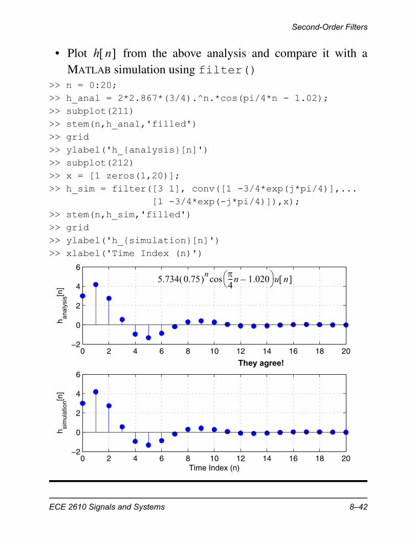
• Plot from the above analysis and compare it with aMATLAB simulation using filter()

>> n = 0:20;>> h_anal = 2*2.867*(3/4).^n.*cos(pi/4*n - 1.02);>> subplot(211)>> stem(n,h_anal,'filled')>> grid>> ylabel('h_{analysis}[n]')>> subplot(212)>> x = [1 zeros(1,20)];>> h_sim = filter([3 1], conv([1 -3/4*exp(j*pi/4)],... [1 -3/4*exp(-j*pi/4)]),x);>> stem(n,h_sim,'filled')>> grid>> ylabel('h_{simulation}[n]')>> xlabel('Time Index (n)')

h n

0 2 4 6 8 10 12 14 16 18 20−2

0

2

4

6

h anal

ysis

[n]

0 2 4 6 8 10 12 14 16 18 20−2

0

2

4

6

h sim

ulat

ion[n

]

Time Index (n)

They agree!

5.734 0.75 n 4---n 1.020– u n cos



Frequency Response

(8.29)

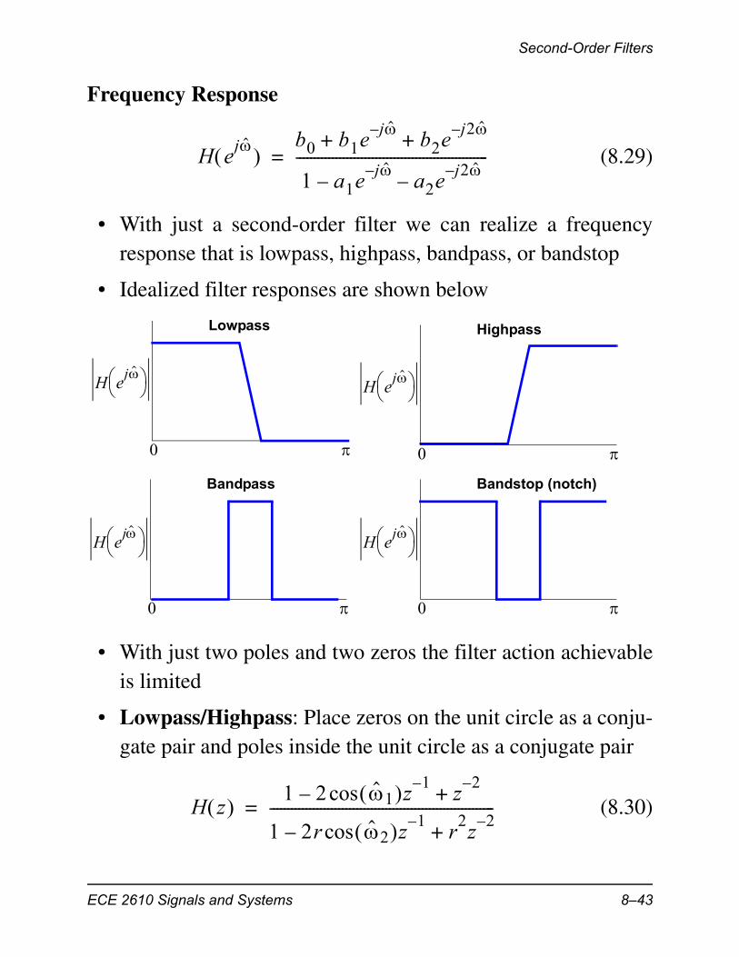
• With just a second-order filter we can realize a frequencyresponse that is lowpass, highpass, bandpass, or bandstop

• Idealized filter responses are shown below

• With just two poles and two zeros the filter action achievableis limited

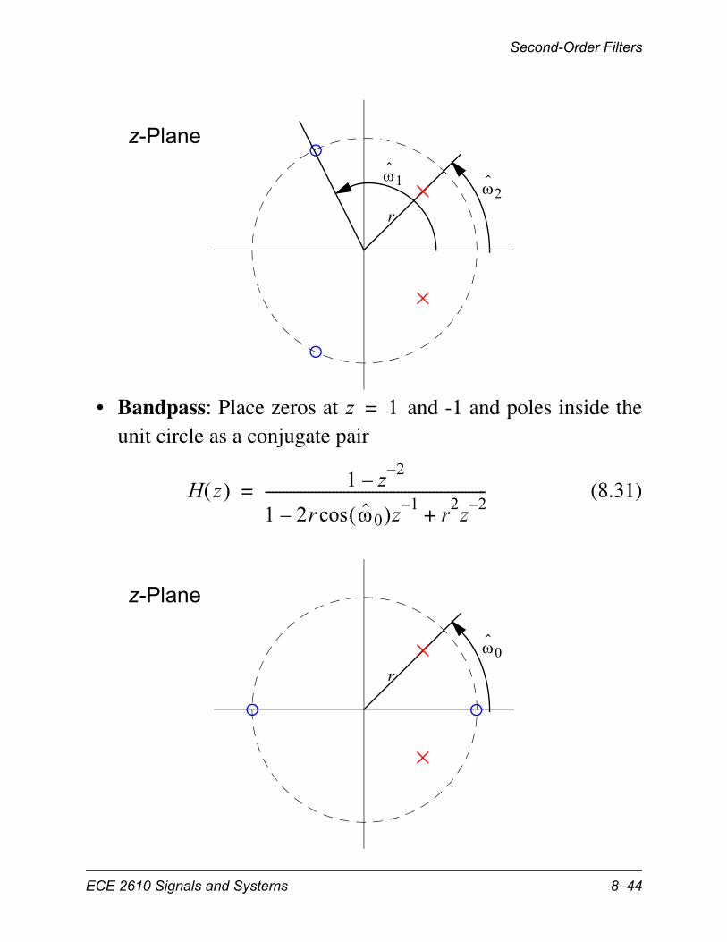
• Lowpass/Highpass: Place zeros on the unit circle as a conju-gate pair and poles inside the unit circle as a conjugate pair

(8.30)

H ej

b0 b1ej–

b2ej2–

+ +

1 a1ej–

a2ej2–

––-----------------------------------------------------=

0

H ej

Lowpass

0

H ej

Highpass

0

H ej

Bandpass

0

H ej

Bandstop (notch)

H z 1 2 1 z 1–

cos– z2–

+

1 2r 2 z 1–cos– r

2z

2–+

--------------------------------------------------------------=



• Bandpass: Place zeros at and -1 and poles inside theunit circle as a conjugate pair

(8.31)

z-Plane

1 2

r

z 1=

H z 1 z2–

–

1 2r 0 z 1–cos– r

2z

2–+

--------------------------------------------------------------=

z-Plane

0

r


Example of an IIR Lowpass Filter

• Bandstop (notch):

(8.32)

– See the final project


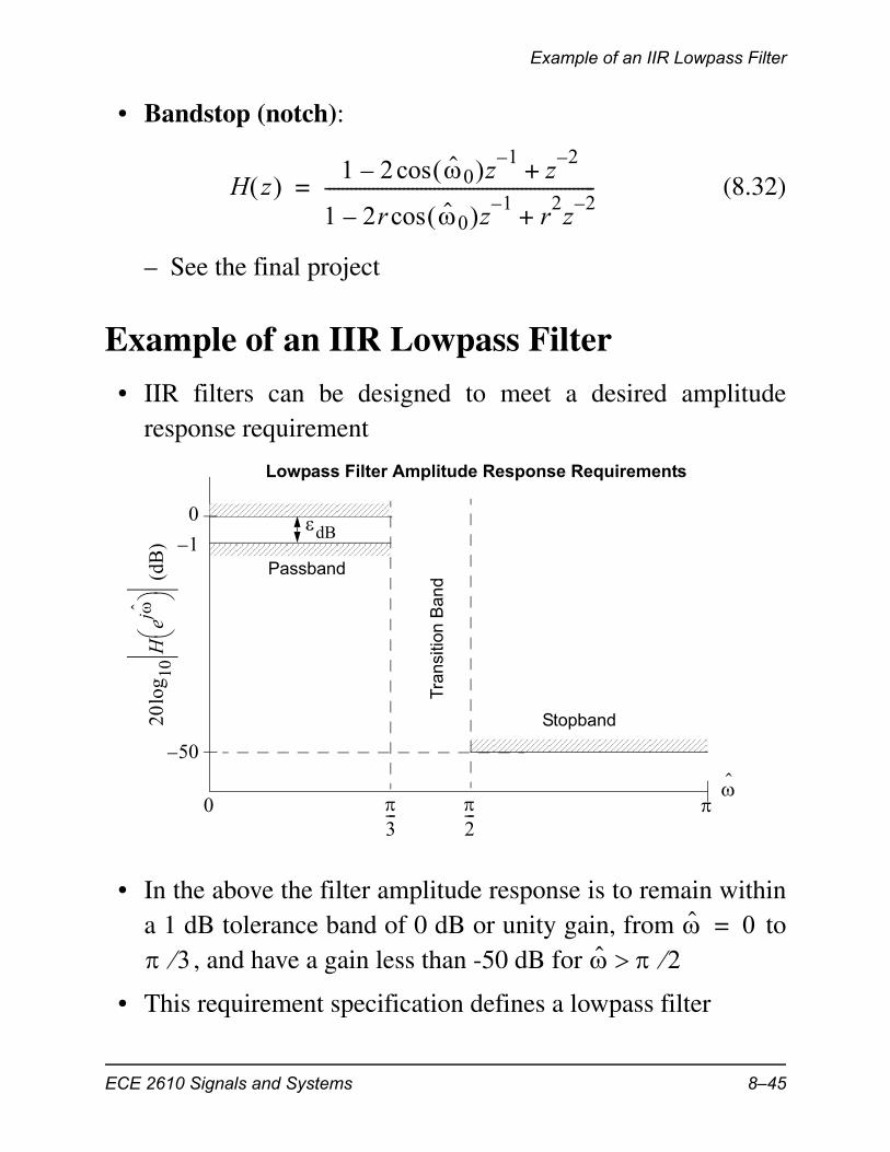
• IIR filters can be designed to meet a desired amplituderesponse requirement

• In the above the filter amplitude response is to remain withina 1 dB tolerance band of 0 dB or unity gain, from to

, and have a gain less than -50 dB for

• This requirement specification defines a lowpass filter

H z 1 2 0 z 1–

cos– z2–

+

1 2r 0 z 1–cos– r

2z

2–+

--------------------------------------------------------------=20

log 10

Hej

(dB

)

0

3---

2---

0

50–

dB

Passband

Stopband

Tra

nsiti

on B

and

1–

Lowpass Filter Amplitude Response Requirements

0= 3 2



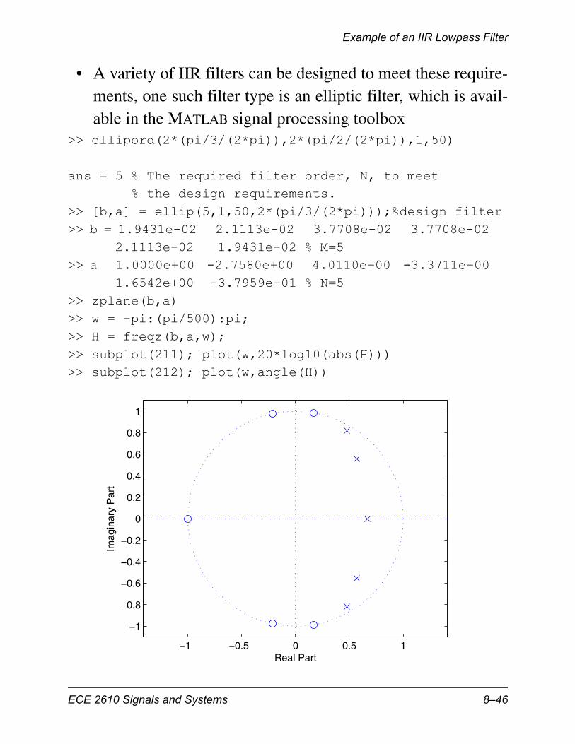
• A variety of IIR filters can be designed to meet these require-ments, one such filter type is an elliptic filter, which is avail-able in the MATLAB signal processing toolbox

>> ellipord(2*(pi/3/(2*pi)),2*(pi/2/(2*pi)),1,50)

ans = 5 % The required filter order, N, to meet % the design requirements.>> [b,a] = ellip(5,1,50,2*(pi/3/(2*pi)));%design filter>> b = 1.9431e-02 2.1113e-02 3.7708e-02 3.7708e-02 2.1113e-02 1.9431e-02 % M=5>> a 1.0000e+00 -2.7580e+00 4.0110e+00 -3.3711e+00 1.6542e+00 -3.7959e-01 % N=5>> zplane(b,a)>> w = -pi:(pi/500):pi;>> H = freqz(b,a,w);>> subplot(211); plot(w,20*log10(abs(H)))>> subplot(212); plot(w,angle(H))

−1 −0.5 0 0.5 1

−1

−0.8

−0.6

−0.4

−0.2

0

0.2

0.4

0.6

0.8

1

Real Part

Imag

inar

y P

art



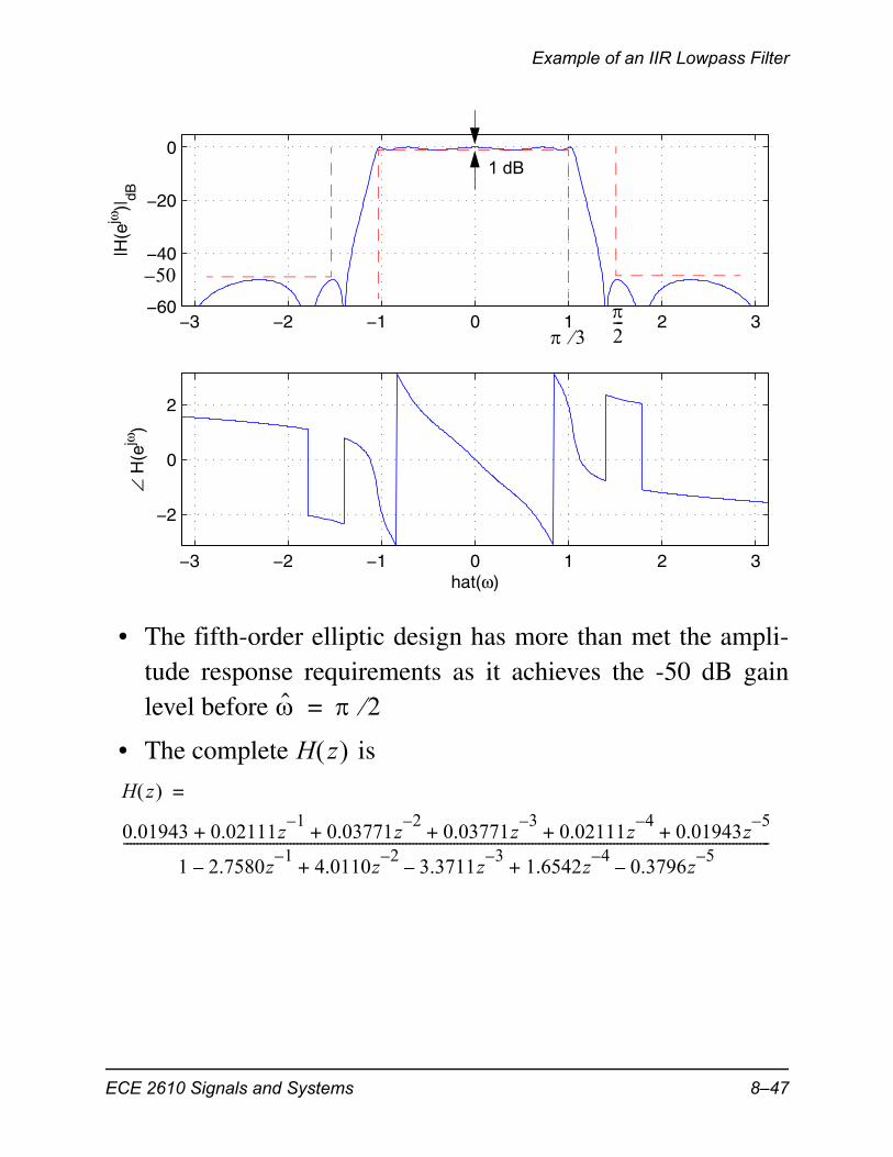
• The fifth-order elliptic design has more than met the ampli-tude response requirements as it achieves the -50 dB gainlevel before

• The complete is

−3 −2 −1 0 1 2 3−60

−40

−20

0

|H(e

jω)|

dB

−3 −2 −1 0 1 2 3

−2

0

2

∠ H

(ejω

)

hat(ω)

32---

50–

1 dB

2=

H z H z =

0.01943 0.02111z1–

0.03771z2–

0.03771z3–

0.02111z4–

0.01943z5–

+ + + + +

1 2.7580z1–

– 4.0110z2–

3.3711z3–

– 1.6542z4–

0.3796z5–

–+ +----------------------------------------------------------------------------------------------------------------------------------------------------------------------------------------------


iir filters chapter

Documents