iii thematic essays - world trade organization - home … · iii thematic essays a quantitative...
TRANSCRIPT

WO
RLD
TR
AD
E R
EPO
RT
200
5III
T
HEM
ATI
C E
SSA
YS
A
Q
UA
NTI
TATI
VE
ECO
NO
MIC
S IN
WTO
DIS
PUTE
SET
TLEM
ENT
171
1 For work in these areas see, for example, Horn et al. (1999), Bown (2002), Leitner and Lester (2003), and Busch and Reinhardt (2003).
2 For instance, no demonstration of trade effects is required in respect of a de jure national treatment violation discernible from the text of the challenged law.
A QUANTITATIVE ECONOMICS IN WTO DISPUTE SETTLEMENT
1. INTRODUCTION
WTO dispute settlement continues to be the subject of extensive scrutiny by both trade practitioners and academics. Not surprisingly, most of this analysis is legal in nature, touching upon the various arguments that have been put forward by parties to disputes and the legal foundations upon which these disputes are adjudicated. While legal and procedural issues remain the domain of trade lawyers, economists are being called upon with increased frequency on matters that call for economic interpretation or quantification. This should hardly be surprising given that multilateral trade rules reflect key economic principles such as comparative advantage, and that many of the terms in WTO Agreements, which are important in the resolution of disputes, have an economic basis. It may also have to do with the fact that increasing numbers of disputes are reaching the implementation phase, in which arbitrators need to quantify the allowable level of retaliation, as will be further explained below.
The literature on economics and dispute settlement is rather limited. A range of studies try to measure the performance to date of the WTO dispute settlement mechanism in one way or another. These include studies on the incentives/disincentives faced by WTO Members to avail themselves of the WTO dispute settlement mechanism and to conform to rulings, as well as more descriptive analyses of the frequency and pattern of recourse to dispute settlement.1 Other contributions have sought to elucidate, from a purely theoretical point of view, various functions of the WTO dispute settlement mechanism, such as deterrence of opportunistic behaviour by governments (Maggi, 1999; Butler and Hauser, 2000). Such institutional aspects of WTO dispute settlement are not the focus of this essay. Nor will economic analyses of the outcome of WTO disputes be discussed, such as the welfare implications of retaliatory measures (Breuss, 2004).
Instead, this essay analyses to what extent quantitative economics has played a role: (i) in the interpretation and application of WTO rules, as to both the consistency and the effects of contested measures; and (ii) in respect of authorized countermeasures, in particular the identification of the maximum allowable level of suspension of concessions, where a party losing a dispute has failed to implement the rulings and recommendations of the Dispute Settlement Body. Although the economic questions to be dealt with may be similar, these two situations are legally quite distinct. In arbitrations over countermeasures, the arbitrators themselves have employed economic models and techniques, whereas in panel/Appellate Body proceedings, it has been the parties, and not the adjudicators, who have undertaken such analysis. In the latter context, if parties include quantitative economic analysis in their arguments, the panels/Appellate Body may or may not find it useful or necessary to their own analysis. In order to distinguish these two types of situations, arbitrations will be addressed in a separate sub-section. This field of research has hitherto been neglected. Closest to describing this type of analysis are probably Sumner et al. (2003), Malashevich (2004), Keck (2004) and aspects of Horn and Mavroidis (2003). This essay does not question the economic rationale of WTO rules, although a good deal could be said about economic sense and nonsense in this context. It does not deal either with the much broader question of how economic concepts and terminology have been used by WTO adjudicating bodies, sometimes implicitly, to structure their reasoning. Instead, this essay simply seeks to identify when, why and in what form quantitative economic analysis has been used at various stages of the WTO dispute settlement process.
Trade disputes at the WTO are about differences in views between Members as to whether or not a specific policy measure of the defending Member contravenes WTO rules. In many cases, the precise effect of a breach of obligations need not be known by the panel.2 An interpretation may be developed based on the ordinary meaning and context of a WTO provision in the light of the object and purpose. And yet, as Neven observes: “To the extent that a legal norm is not solely based on forms and relies on an assessment of the effects of any particular measure, economic analysis will be instrumental in its implementation” (Neven, 2000, p.3).
III THEMATIC ESSAYS

WO
RLD
TR
AD
E R
EPO
RT
200
5III
T
HEM
ATI
C E
SSA
YS
A
Q
UA
NTI
TATI
VE
ECO
NO
MIC
S IN
WTO
DIS
PUTE
SET
TLEM
ENT
172
Indeed, certain WTO disciplines, for example in the Agreement on Subsidies and Countervailing Measures (SCM), provide for action based on the effects of subsidies. This essay concentrates on instances where a quantification of trade effects, as well as other economic conditions such as the competitive relationship within a given market, has come into play during panel/Appellate Body proceedings. In addition, as mentioned above, once a dispute has reached the implementation stage, the issue of countermeasures has been found in some cases to require an estimate of the effects that the offending measures have on trade.
The main objective of this Section is to examine the way in which quantitative economic analysis has been used during WTO dispute settlement proceedings. To that end, WTO cases that have proceeded at least to the Appellate Body stage have been reviewed and principal illustrative examples of the use of quantitative economic analysis at any stage of the adjudication process identified.3 For the purposes of this essay, “quantitative economics” shall simply refer to attempts to measure the relationship between economic variables, including trade flows. Quantifying the effects that one variable has on another, and isolating these effects from other influences, is usually based implicitly on some form of theoretical economic model and requires a minimum of relevant data and reliable parameter estimates. In that sense, “quantitative economics” shall be understood to go beyond simple accounting operations or the use of descriptive statistics in order to characterize economic phenomena.
The essay contains four more Sections. The next Section (Section 2) identifies some questions common to disputes where quantitative economic analysis has occurred. The third Section explains briefly basic economic techniques to address such questions. The fourth Section illustrates the actual use of quantitative economics in selected WTO cases. The concluding Section summarizes observations on the possibilities and limitations of using quantitative economics in WTO dispute settlement.
2. THE CONTRIBUTION OF QUANTITATIVE ECONOMIC ANALYSIS TO LEGAL QUESTIONS IN WTO DISPUTE SETTLEMENT
A good starting point to examine the contribution that quantitative economics can make to WTO dispute settlement is to see when it has actually been used and why. So far, quantitative economic analysis seems to have been applied to find answers to two major questions implicit in a number of WTO provisions. The first concerns the effect of a policy measure (or its removal) on trade flows. Precise trade values may be required, or the trade impact of a more indirect measure may be assessed to see how, for example, the measure had affected world prices. This type of issue can arise either in the context of a determination by a panel and/or the Appellate Body whether a violation has occurred, or in the context of determining the level of authorized countermeasures, where a losing party has not implemented the dispute settlement findings. The second question concerns the effect of imports on competing domestic products or their producers. This type of issue may typically arise in the process of determining a violation. For example, in a discrimination case, the degree of competition between two products may be at issue and if it is not significant, the two products may be seen as not belonging to the same relevant market (and could, for instance, be regulated differently).4 Alternatively, as in a WTO challenge of a trade remedy measure, it may be necessary to review how the relevant national authorities separated the effect of imports on prices, profitability, sales and other indicators of the health of a domestic industry from the effects that other factors, such as developments in technology/
3 Evidently, every case in which a violation is found, whether appealed or not, eventually is adopted by the Dispute Settlement Body (DSB) – by the reverse consensus rule – and thus creates a requirement that the losing party implement the DSB’s rulings and recommendations. The review of cases for the purposes of this essay was “artificially” limited to those in which appeals took place in order to keep the task within manageable dimensions. This undertaking is modest in nature confining itself to a simple stock-take and ex post analysis of some of the existing case law. The actual examples will be used to further explain some of the analytical tools commonly employed by economists. Some issues relating to data and underlying assumptions will also be highlighted. Clearly, the intention of this essay is not to rewrite WTO case law nor to adopt a prescriptive stance on the use of quantitative economics.
4 It is important to note that, here, quantitative economics may be used to determine the degree of direct competition or substitutability. Once that is established, no precise assessment of the trade effects may be necessary for a violation finding if, for instance, a de jure discriminatory treatment derives from the text of the challenged measure itself.

WO
RLD
TR
AD
E R
EPO
RT
200
5III
T
HEM
ATI
C E
SSA
YS
A
Q
UA
NTI
TATI
VE
ECO
NO
MIC
S IN
WTO
DIS
PUTE
SET
TLEM
ENT
173
productivity or changes in demand, may have had on those variables. This last question is not unrelated to the preceding one, but the focus is less on the degree of competition from imports and more on the need to ensure that other influences have not been falsely attributed to imports.
(a) Effect of policy measures on trade
Qualitative explanations of the existence of an effect of a measure, where this is necessary to show a violation of trade rules, may often be sufficient to resolve a dispute. Why, then, has it sometimes been seen as advantageous by parties to inform economic insights through quantifiable information? And why have arbitrators in certain cases employed quantitative trade models to estimate the allowable level of suspension of concessions? In arbitration cases under Article 22.6 of the Dispute Settlement Understanding (DSU), a quantification of counterfactual trade effects has been a key device for some arbitrators to fulfil their mandate – namely, to determine the level of nullification or impairment of benefits suffered by a complaining Member, which the requested suspension of concessions or other obligations must not exceed. Some parties have provided quantitative economics or were solicited by arbitrators to do so, which the latter used to varying degrees in their own analysis. Examples also include the areas of prohibited and actionable subsidies, where arbitrators have faced the special mandate under the SCM Agreement to decide whether the countermeasures proposed are, respectively, “appropriate” or “commensurate” with the adverse effects found. Arbitrations may occur in relation to any WTO Agreement and, potentially pose challenging questions, for instance, in regard to the quantification of non-tariff measures and their effects.
Apart from the concrete mandate given to arbitrators, the issue of measuring the effect of policy measures on trade has also been brought up on occasion by parties during panel proceedings. Here, quantitative economic analysis formed part of parties’ argumentation in order to give an indication of the extent to which a disputed measure diminished a Member’s benefits in terms of lost trading opportunities. This is a key question in claims of “serious prejudice”, which is one of the adverse effects to a Member’s interests that may emanate from “actionable” subsidies. The concrete questions that may arise in such cases include whether such a subsidy displaces or impedes the exports of the complaining Member or leads to significant price undercutting, price suppression/depression or lost sales in the same market.
(b) Effect of imports on domestic products/producers
As far as the effect of imports on competing domestic products or their producers is concerned, parties have at times seen an advantage in using quantitative economics, for instance, to sustain or ward off claims of tax discrimination against foreign products to the benefit of domestic producers. As a prerequisite for such claims, imported and domestic products need to be in a competitive relationship. If products were unrelated and therefore were not in competition in the market, they could well be treated differently. While adjudicating bodies in these and similar cases have relied on qualitative criteria, such as physical properties of the products or the extent to which the products were capable of serving the same or similar end-uses as well as consumer perceptions, the competitive pressure two products exert upon one another is ultimately a matter of degree. In related fields, such as anti-trust investigations, an essential measurement tool is the cross-impact (elasticity) on price. There are a few WTO cases where parties have seen merit in providing empirical evidence of the intensity of competition, notably by estimating cross-price elasticities.
From a different angle, the competitive pressure exerted by imports is of key importance in investigations of injury of a domestic industry, the results of which may be challenged at the WTO. In particular, to apply a WTO-consistent trade remedy, the national authorities involved need to determine, on the basis of an investigation conducted in accordance with the applicable WTO rules, that dumped or subsidized imports or import surges, as opposed to other factors, cause injury to a domestic industry (so-called “causation” and “non-attribution” analysis). Both the procedural and substantive aspects of such a determination can be the subject of WTO dispute settlement.5
5 As described in more detail below, WTO dispute settlement in respect of anti-dumping determinations is subject to a special standard of review.

WO
RLD
TR
AD
E R
EPO
RT
200
5III
T
HEM
ATI
C E
SSA
YS
A
Q
UA
NTI
TATI
VE
ECO
NO
MIC
S IN
WTO
DIS
PUTE
SET
TLEM
ENT
174
In sum, quantitative economic analysis is bound to occur with most regularity in WTO arbitrations due to their specific mandate and the need to make a precise award that in most cases must be quantified, often with reference to the effects of the inconsistent measure. That said, during regular panel proceedings, where the question is the existence of an inconsistency with a WTO provision, parties may include quantitative economic analysis in their submissions whenever they deem it necessary or required under the respective agreements to show how seriously a domestic policy impacts on trade or how imports relate to developments in domestic factors. Panels need not ascribe the same evidentiary weight or draw the same legal or factual conclusions from quantitative economics as the party submitting it.6 This is clearly expressed in the view of the panellists in Korea–Alcoholic Beverages,7 who stated that “quantitative analyses, while helpful, should not be considered necessary” (Korea–Alcoholic Beverages, Panel Report: para. 10.42).8 Before discussing a representative range of cases where quantitative analysis has been used, we shall briefly review some relevant economic techniques and terminology.
3. TRADE MODELS: SPECIFICATION AND PARAMETERS
Intuitive understanding of economic relationships – say, for example, consumers buy less of a product when it becomes more expensive – is often based implicitly on an economic model. In our simple example, the idea is of a general loss in purchasing power and substitution to other products.9 Why formalize such relationships? Most importantly, because one may wish to identify the relationship with more precision. For a given price increase, for example, by how much will the quantity demanded fall? In addition, formalization forces the analyst to be explicit about assumptions, simplifications and presumed relationships. It helps to prevent omission of important linkages and misguided impressions about the relative importance of individual factors. Finally, the quality of a formal model can be measured in terms of the degree of confidence one can have in its result. This Section provides a basic introduction into technical aspects of trade model-building. These technical characteristics can be the subject of controversy if models form part of parties’ submissions in a dispute. Although a wide range of trade models exist, and some of them can become quite complex, the focus of the discussion here will be on basic aspects of models that may be relevant in dispute settlement.
(a) Model specification
Trade models combine information on trade flows and trade policy measures for different product categories in a structured manner. They can then be used to show to what extent outcomes are sensitive to assumptions and policy changes and, therefore, are a useful tool to evaluate competing conjectures about potential trade impacts of a measure. While many trade models focus on import market conditions only, recent approaches have included global market clearing conditions, and, subject to data availability, domestic production (Francois and Hall, 2003).
Trade models are commonly used to evaluate how a change in trade policy may affect prices and consequently trade flows. By the same token, trade may also feature in a model as one determinant of other economic variables of interest, such as prices, output and employment. A quantitative model consists of one or several equations that relate different economic variables to one another. In the simplest case, a model is made of just one equation, which explains one variable as a function of one or several other variables. In models consisting of a set of equations a variable of interest may be a function of several other variables that are related to each other as well. This allows for a more realistic set-up, as, usually, variables are interdependent and causality goes in both directions. Besides such “behavioural equations”, multi-equation models contain accounting identities that link the behavioural equations to one another. Usually,
6 It should be noted that there are no evidentiary rules under the DSU constraining the type of admissible evidence. Parties to disputes are free as to the type of evidence they submit, as they are presumed to act in good faith. Panels are free to admit evidence and assign weights to it as they see fit. There are, of course, requirements to submit specific evidence in, for instance, anti-dumping and countervailing duty investigations. For more see Anderson (2004).
7 Throughout the essay, the short titles for WTO dispute settlement cases are used. For full case titles and citations, see Appendix Table 1.
8 See also Korea – Alcoholic Beverages, Appellate Body Report: paras. 109 and 131. In this report, the Appellate Body discussed the terms “directly competitive or substitutable” quite extensively from an economic perspective.
9 More precisely, in this case, there is a loosely conceived idea that the loss in purchasing power associated with a price increase reinforces substitution away from the more expensive good. However, if the product in question is inferior, the reduction in real income leads to an opposite income effect that may well outweigh substitution tendencies and lead to an overall increase in demand (“Giffen good”).
WO
RLD
TR
AD
E R
EPO
RT
200
5III
T
HEM
ATI
C E
SSA
YS
A
Q
UA
NTI
TATI
VE
ECO
NO
MIC
S IN
WTO
DIS
PUTE
SET
TLEM
ENT
175
there are a number of possibilities to construct a model, and the burden of additional data collection and estimation difficulties for added variables or multi-equation systems have to be compared to the expected gains in precision.10
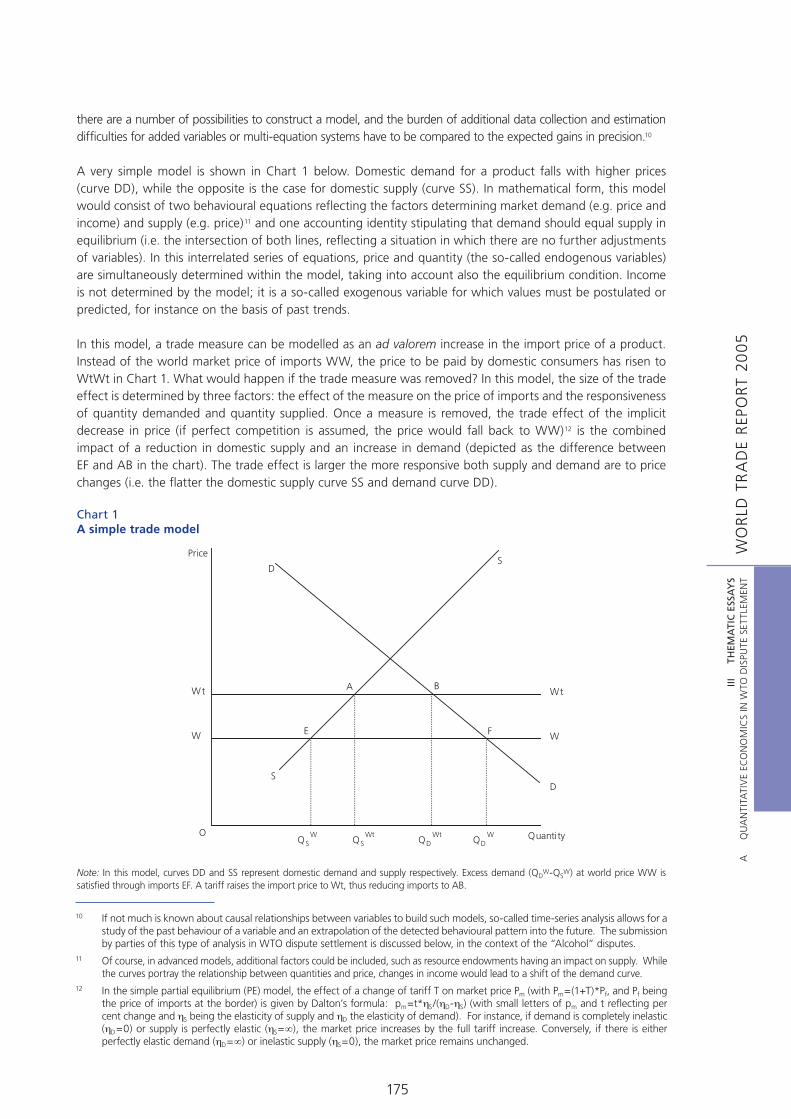
A very simple model is shown in Chart 1 below. Domestic demand for a product falls with higher prices (curve DD), while the opposite is the case for domestic supply (curve SS). In mathematical form, this model would consist of two behavioural equations reflecting the factors determining market demand (e.g. price and income) and supply (e.g. price)11 and one accounting identity stipulating that demand should equal supply in equilibrium (i.e. the intersection of both lines, reflecting a situation in which there are no further adjustments of variables). In this interrelated series of equations, price and quantity (the so-called endogenous variables) are simultaneously determined within the model, taking into account also the equilibrium condition. Income is not determined by the model; it is a so-called exogenous variable for which values must be postulated or predicted, for instance on the basis of past trends.
In this model, a trade measure can be modelled as an ad valorem increase in the import price of a product. Instead of the world market price of imports WW, the price to be paid by domestic consumers has risen to WtWt in Chart 1. What would happen if the trade measure was removed? In this model, the size of the trade effect is determined by three factors: the effect of the measure on the price of imports and the responsiveness of quantity demanded and quantity supplied. Once a measure is removed, the trade effect of the implicit decrease in price (if perfect competition is assumed, the price would fall back to WW)12 is the combined impact of a reduction in domestic supply and an increase in demand (depicted as the difference between EF and AB in the chart). The trade effect is larger the more responsive both supply and demand are to price changes (i.e. the flatter the domestic supply curve SS and demand curve DD).
Chart 1A simple trade model
Note: In this model, curves DD and SS represent domestic demand and supply respectively. Excess demand (QDW-QS
W) at world price WW is satisfied through imports EF. A tariff raises the import price to Wt, thus reducing imports to AB.
Quanti ty
A B
FEW
Wt
QSW
QSWt
QDWt
QDW
Wt
W
O
PriceS
D
SD
10 If not much is known about causal relationships between variables to build such models, so-called time-series analysis allows for a study of the past behaviour of a variable and an extrapolation of the detected behavioural pattern into the future. The submission by parties of this type of analysis in WTO dispute settlement is discussed below, in the context of the “Alcohol” disputes.
11 Of course, in advanced models, additional factors could be included, such as resource endowments having an impact on supply. While the curves portray the relationship between quantities and price, changes in income would lead to a shift of the demand curve.
12 In the simple partial equilibrium (PE) model, the effect of a change of tariff T on market price Pm (with Pm=(1+T)*Pf, and Pf being the price of imports at the border) is given by Dalton’s formula: pm=t*ηS/(ηD-ηS) (with small letters of pm and t reflecting per cent change and ηS being the elasticity of supply and ηD the elasticity of demand). For instance, if demand is completely inelastic (ηD=0) or supply is perfectly elastic (ηS=∞), the market price increases by the full tariff increase. Conversely, if there is either perfectly elastic demand (ηD=∞) or inelastic supply (ηS=0), the market price remains unchanged.

WO
RLD
TR
AD
E R
EPO
RT
200
5III
T
HEM
ATI
C E
SSA
YS
A
Q
UA
NTI
TATI
VE
ECO
NO
MIC
S IN
WTO
DIS
PUTE
SET
TLEM
ENT
176
In the Chart, it is also assumed that the reduction in imports due to the trade measure is small at the global level and does not affect world price. But an additional complication arises if, for example, the importing country is large and the contraction in imports causes the world price to fall. In this case, once the measure is removed, the effect on imports would be smaller than before due to a simultaneous rise in the world price. Also, imports and domestically produced goods are not necessarily perfect substitutes, and specific import demand elasticities need to be considered. If these are low, i.e. consumers do not consider an imported product to be a close substitute for a domestically produced good, the effects of a removal of trade barriers will be scaled down accordingly.
In partial equilibrium (PE) models like the one described above, cross-price effects in other markets are ignored as well as overall resource limitations and budget constraints. Conversely, general equilibrium (GE) analysis seeks to portray all linkages in the economy. For instance, an additional tax on alcoholic beverages may lead to a higher consumption and, consequently, production of soft drinks, additional demand for sugar as a key ingredient and, ultimately a shift of labour out of the alcohol industry into the soft drink and sugar sectors. These shifts may affect the income of households and, subsequently, their consumption patterns, which may trigger another round of feed-back effects in the economy.
In PE models, linkages between the sector modelled and the rest of the economy are deliberately left out in order to be able to reduce the amount of data needed, conduct the study at a more disaggregated level, and concentrate on the direct impact of specific policies only. In many cases, multi-commodity PE frameworks are entirely adequate, especially if the sector studied is small in relation to overall economic activity (Hertel, 1990).13
An important distinction must be made between the estimation of a model and simulations carried out using the model. Estimation refers to the determination of the individual parameters (elasticities, for example; see below) that quantify the impact of each factor on the variable under study.14 A range of techniques of varying complexity exist to establish these dependencies, or, in the jargon, to “regress” a “dependent” variable on a set of “explanatory” variables.15 Key criteria to be considered in choosing an appropriate regression technique and in interpreting the results will be further illustrated below in the discussion of some WTO disputes, where this was an issue. The resulting parameters give an indication of the specific influence of a factor on the variable under study, other things being equal.16
With estimated values for the parameters of a model, the initial (i.e. baseline) values for the endogenous (dependent) variables and a given time path for the development of the exogenous (independent) variables, the model can then be used to produce a forecast of the endogenous variables over that time period. Or individual exogenous variables controlled, say, by the government (e.g. taxes leading to reductions in disposable income) can be modulated in order to assess their impact on the target variable. This also has the advantage that the effects of individual policies can be predicted in isolation and compared to alternative options. These types of analyses are called simulations. Besides the nature of the policy change (and other assumptions about exogenous variables), the results of simulations are driven by the structural specification of the model (i.e. the chosen functional form and range of variables included) and the estimated behavioural parameters. In trade models, which often follow fairly standard theoretical structures, the latter account for much of the variation amongst the results of different studies.
13 Both GE and PE models are often of a “comparative static” nature, i.e. comparing an initial situation (“equilibrium”) to the one after the economic environment has changed. The time path and adjustment process, i.e. the dynamic features of change, are not modelled.
14 Ideally, an empirical model is based on economic theory. This is not always the case. But even if it is, it may be estimated in a so-called “reduced form” that may not allow for an identification of all of the parameter values of the underlying structural model.
15 If there are mutual dependencies, all parameters in a system of equations must be estimated simultaneously, adding considerable complexity to the estimation procedure.
16 More precisely, the parameters reflect an estimation of the average value of the dependent variable for known values of the explanatory variables.

WO
RLD
TR
AD
E R
EPO
RT
200
5III
T
HEM
ATI
C E
SSA
YS
A
Q
UA
NTI
TATI
VE
ECO
NO
MIC
S IN
WTO
DIS
PUTE
SET
TLEM
ENT
177
(b) Elasticity parameters
Trade model parameters are commonly expressed in the form of elasticities. An elasticity represents the percentage change of one variable in response to a one per cent change in another variable, all other things being equal. Elasticities are rooted in micro-economic theory and reflect the sensitivity of consumers and firms to changes in relative prices and income.17 The basic elasticity expressions (price, income and substitution elasticities) are explained in Box 1. Elasticity values are not normally known with precision. The elasticity of demand for a given product, for instance, i.e. the percentage change in quantity demanded induced by a one per cent price change, may differ according to the econometric method employed, the quality of the historical price and quantity data as well as the number of variables included or held constant in the basic economic framework used for the estimation. Elasticities are so-called “local” parameters, i.e. valid only in a given situation of prices and income. In a different initial situation values may be altered. The term “trade elasticities” in the literature usually refers to expressions that are price or income elasticities of imports or exports, or elasticities of substitution between home and foreign or different foreign goods. For example, the own price elasticity of car imports is often referred to as the “import demand elasticity for cars.”
17 However, in empirical work, the supply and demand equations sometimes may not be derived from explicit assumptions about producer and consumer behaviour (Hertel, 1990).
Box 1: Main types of elasticities
Own-price and cross-price elasticity
The own-price elasticity of a product specifies the responsiveness (in per cent) of the demand for that good to an increase in its price by one per cent. In this case, it may be called a demand elasticity, which, typically, is negative. In case of producers, who normally are willing to sell more when prices rise, the own-price elasticity, or supply elasticity, is positive. Economists speak of “elastic” (or “inelastic”) behaviour. This refers to cases when the absolute value of an elasticity is above (elastic) or below (inelastic) unity. In the above example, demand is said to be more elastic if the quantity demanded falls by, for instance, 2 per cent (elasticity of -2) in response to a one per cent price increase than if it falls by 1.5 per cent only (elasticity of -1.5). In many instances, consumers not only buy less of a product the price of which has increased (the so-called “own-price elasticity” described above), but, as a consequence, buy more of a substitute. For instance, if the price of butter increases by one per cent, consumers may wish to eat more margarine instead, leading to a, say, one half of a per cent increase in its demand. The cross-price elasticity expresses by how much (in per cent) the demand for a product (margarine) changes in response to a one per cent price increase of another product (butter). It is positive if two products are substitutes, and negative if they are complements. The latter is the case, for instance, when a price increase (and hence reduced demand) in automobiles leads to a lower demand in car radios.
Income elasticity
This concept describes the percentage change in demand for one good in response to a one per cent increase in income. Normally, one would assume that someone who has consumed a certain “mix” of products continues to do so at a higher income, at increased quantities of each product (perhaps with a slightly different allocation of spending across commodities). Hence, the income elasticity of a normal product is positive. However, it may also be that, at higher income levels, a consumer can afford to buy so much more of, say, truffles pasta that she wishes to eat less of a product she consumed before, such as potatoes. For such inferior goods, the income elasticity may be negative. Price and income elasticities together are key parameters in describing demand for a good.

WO
RLD
TR
AD
E R
EPO
RT
200
5III
T
HEM
ATI
C E
SSA
YS
A
Q
UA
NTI
TATI
VE
ECO
NO
MIC
S IN
WTO
DIS
PUTE
SET
TLEM
ENT
178
Elasticity of substitution
The elasticity of substitution is closely related to the concept of cross-price elasticity. It has its origins in the theory of the firm characterizing firms’ demand for different combinations of production factors (“inputs”) to obtain a given output, subject to the technology used and cost structure of the firm. The elasticity of substitution (often denoted as σ (“sigma”)) has a slightly different mathematical form than the above elasticity types, measuring how the ratio of two inputs responds to a change in the relative price of those two inputs (Varian, 1984). If the response is positive, substitution becomes more important the larger it is. If it is negative, the two goods are said to be complements. When there are more than two factors of production, one also needs to ask how those vary if relative prices change. For simplicity, total production is often considered to consist of production activities of several branches. Hence, elasticities of substitution often reflect the substitution effects within a branch, holding branch output constant (Keller, 1980). Elasticities of substitution are also used in the context of final consumer demand. They obviate some problems associated with direct price elasticity estimation, but are subject to a number of limiting assumptions concerning income and price elasticities of demand for the respective products. Essentially, this implies that the two commodities for which a substitution elasticity is estimated must be considered alike in all economic respects except that they are not perfect substitutes (Stern et al., 1976). In world trade models, this is a convenient assumption for products that are seen as imperfect substitutes owing solely to their difference in origin. The mathematical specification as a relationship between changes in volume and price ratios can reflect the change in market shares, which may be of more interest than changes in absolute levels of sales if the whole market expands/shrinks simultaneously.
Trade elasticities are key parameters in trade policy modelling. They are the nexus between trade policies on the import side and the domestic economy (Francois and Reinert, 1997). The most prominent types are the Armington elasticity of substitution and import demand elasticity.
(i) Armington elasticities
An Armington elasticity has to do with the notion that similar domestic and imported goods, as well as goods imported from different origins, should be regarded as imperfect substitutes. Trade models usually take this into account and differentiate goods by their country of origin, an idea originally proposed by Armington (1969).18 The effect of a trade policy measure on the relative price of similar traded and domestically produced goods leads to a substitution of domestic for imported goods or vice versa, or to a substitution between imports from different sources. The Armington elasticity normally has the form of a substitution elasticity (i.e. percentage change in relative quantities of two products from different origin divided by the percentage change in relative prices – see Box 1). Many trade models working with Armington elasticities assume a two-tiered process, whereby a change in relative prices leads first to substitution between the domestic and foreign commodity. Once the overall level of imports of that commodity is determined, substitution among foreign suppliers is considered. Conventionally, the Armington elasticity of the second tier is set at twice the value of the first tier elasticity (Donnelly et al., 2004). Comprehensive studies at the industry level exist, mostly for the United States (McDaniel and Balistreri, 2002, provide an overview), but these have subsequently been applied to other countries (see, for instance, Donnelly et al., 2004).19
18 In order to describe preferences among goods of different origin, Armington used a functional form implying a constant elasticity of substitution (CES), i.e. one that is independent of initial values. For this and other reasons, the Armington assumption has been subject to academic controversy, which, among other things, led to an alternative approach of firm-level product differentiation. The latter approach has the advantage of depicting the real world more accurately and minimizing terms-of-trade effects inherent in the Armington structure. However, owing to the scarcity of available firm-level data, sector- and region-specific product weights are often used resulting in an Armington-like approach (Francois and Reinert, 1997).
19 It is, of course, preferable to determine elasticities based on historical data and to use econometric methods that are consistent with economic theory, like for instance Kee et al. (2004). The elasticities in Donnelly et al. (2004) have been derived from a range of existing studies. The authors have then employed the expertise of industry analysts to make appropriate adjustments to some of the elasticities found in the literature.

WO
RLD
TR
AD
E R
EPO
RT
200
5III
T
HEM
ATI
C E
SSA
YS
A
Q
UA
NTI
TATI
VE
ECO
NO
MIC
S IN
WTO
DIS
PUTE
SET
TLEM
ENT
179
(ii) Import demand elasticities
The demand for imports is derived from the excess of domestic demand over domestic supply. The import demand elasticity usually takes the form of an own-price elasticity that indicates by how much import volumes adjust if import prices increase, e.g. due to a tariff hike. Imperfect substitutability between imports and domestic products is normally presumed to exist.20 Apart from price, import demand functions used for estimation normally include other variables, such as income, prices of other domestic goods and domestic supply factors, such as resource endowments that may influence the result.21 Some studies have estimated in similar ways export supply elasticities or income elasticities of both imports and exports to make predictions over the direction in which the trade balance of a country may move (e.g. Houthakker and Magee, 1969). Much effort has gone into such estimations, and increasingly the need was seen to focus on higher levels of disaggregation, where trade policies are usually determined. Kee et al. (2004) have conducted estimations of more than 300,000 import demand elasticities for 117 countries. Other authors have focused increasingly on bilateral trade relationships in order to reflect more accurately the sensitivity of the direction of trade to changes in import prices and income (Marquez, 1990).
All of these studies generally find a wide variability of trade elasticities across sectors and frequently arrive at a range of values for any particular sector. In view of different underlying assumptions, not all estimations can be meaningfully compared.22 Marquez (1999) finds an explanation even for a dispersion of estimates that rely on the same constant elasticity model. A few observations common to all trade elasticity estimations can, however, be made (McDaniel and Balistreri, 2002; Kee et al., 2004), in particular, that the level of product aggregation is important, as trade elasticities are higher at lower levels of aggregation (i.e. switching from cotton shirts to wool shirts is easier than from shirts and pants). Therefore, the application of aggregate elasticities to individual sectors or of the average elasticity from disaggregate estimates to an aggregated commodity would lead to an under- or over-estimation of results respectively. Trade simulation models, especially when they are of a GE nature, often derive their elasticity values from a variety of specialized econometric studies, that may be limited to certain countries or sectors and may not involve the same functions in their estimation as those making up the simulation model. In addition, the sample period used in the estimation may not correspond to the date of the baseline scenario in the simulation model (Huff et al., 1997). These and other divergences may make it necessary to perform adjustments to render these elasticities model-consistent, probably at the cost of increased uncertainty about their true value. This is why a systematic sensitivity analysis with plausible elasticity values is advisable, and this will yield a range of possible model outcomes.
4. QUANTITATIVE ECONOMIC ANALYSIS IN SELECTED DISPUTE SETTLEMENT CASES
This Section will first, in Sub-section (a), discuss how the issue of measuring the effect of policy measures on trade has been dealt with in WTO arbitrations. In arbitrations, the consistency with WTO obligations is no longer at issue, and quantitative economic analysis has been applied by some arbitrators in order to determine the level of countermeasures. Sub-section (b) then gives examples from panel proceedings, where quantitative economics has been used to answer the questions mentioned in Section 2. The issue of the effect of a policy measure on trade will be discussed in relation to claims of serious prejudice caused by
20 If domestic and imported goods are not considered close substitutes, as is commonly the case in trade models incorporating the Armington assumption, import demand elasticities can be estimated in their own right. Otherwise, domestic demand and supply elasticities should be estimated and combined with information on production and consumption in the exporting country. See Stern et al. (1976) and Stern (1973).
21 Although both demand and supply factors influence prices and quantities and, hence, a system of equations should be estimated simultaneously, there is relatively little research incorporating the supply side. For an overview see Stern et al. (1976). Only recently have researchers, such as Kee et al. (2004) who treated imports as inputs into production rather than final goods to reflect increasing vertical specialization in today’s global economy, taken into account supply side shifts associated with the reallocation of resources due to changes in prices and primary production factors.
22 Elasticities in GE models have to be interpreted with particular care. While elasticities are, by definition, partial equilibrium phenomena, the model also produces so-called unconditional or GE elasticities, when all endogenous variables are permitted to adjust to their new equilibrium following a policy intervention. See Hertel et al. (1997) for a detailed explanation.

WO
RLD
TR
AD
E R
EPO
RT
200
5III
T
HEM
ATI
C E
SSA
YS
A
Q
UA
NTI
TATI
VE
ECO
NO
MIC
S IN
WTO
DIS
PUTE
SET
TLEM
ENT
180
subsidies, i.e. adverse effects suffered in variously-defined markets, due to subsidies. Then examples from disputes will be highlighted, where the relationship between imports and domestic products/producers was analysed economically. One example deals with disputes in regard to alleged tax discrimination and one with disputes involving the application of trade remedies. Here, relevant legal concepts that have given rise to the presentation of quantitative economic analysis in the context of WTO dispute settlement are whether the domestic and imported products at issue are directly competitive and substitutable, and whether causation/non-attribution of injury in the context of trade remedy investigations has been properly performed.
(a) WTO-inconsistent measures and arbitration on proposed countermeasures under DSU Article 22.6: effect of policy measures on trade
Nine arbitrations pursuant to DSU Article 22.6 have taken place so far.23 In certain of these cases, the arbitrators have opted to use quantitative economic analysis to carry out their mandated tasks. The arbitrations to date, which have involved requests for multi-million dollar awards, have been undertaken on the basis of one of two mandates.24 The first is pursuant to DSU Article 22.7 (in connection with Articles 22.4 and 22.6), under which the arbitrators’ principal duty is to ensure that the retaliation sought by a complaining Member is equivalent to the level of nullification or impairment that has arisen from the breach of WTO obligations.25 The key challenge for arbitrators usually lies in determining what trade flows would have been but for the unlawful measure. So far, this so-called “trade effects approach” that equates nullification or impairment with the value of trade foregone has been the principal tool used to determine the final arbitration award. In so doing, arbitrators can either agree with the requested amount, or disagree and establish another level.26
The second mandate under which arbitration has been conducted to date is that covering prohibited export subsidies. Here, the relevant standard (Subsidies and Countervailing Measures (SCM) Agreement Articles 4.10 and 4.11) requires arbitrators to assess whether proposed countermeasures are “appropriate” as a response to the initial wrongful act and (according to footnotes 9 and 10) “not disproportionate” in light of the fact that the subsidies are prohibited.27 In all three cases that have been adjudicated under Article 4.11 of the SCM Agreement, reference has always been made to the standard of “nullification or impairment” as stated in Article 22.4 of the DSU and its inapplicability to cases under SCM Article 4.10. It has also been stated that where trade concepts are explicitly contemplated they are defined in other parts of the Agreement.28 The lack of precision arising from the term “appropriate” has implications for the consistency of the standard to be used by arbitrators across cases. This point is recognised by the Arbitrator in the Foreign Sales Corporations (FSCs) case who states that “countermeasures should be adapted to the particular case at hand”.29 The Arbitrator goes further by stating that “there is an element of flexibility, in the sense that there is thereby an
23 A number of articles on the WTO arbitration process have been published, most of which focus on the need for arbitration to ensure a viable dispute settlement process and the unique nature of the WTO’s approach compared to other arbitration procedures (Lawrence, 2003; Bagwell and Staiger, 2002). Again, despite a growing literature, the role of economics in the arbitration process has received much less attention than the economics of arbitration. A few articles on the latter issue that have stressed the difference between welfare analysis and trade analysis may also be relevant in relation to the use of economics in arbitration (Anderson, 2002; Bernstein and Skully, 2003).
24 It should be noted that the key objective under both mandates is compliance with the original ruling. Arbitration is not supposed to result in “punitive” measures.
25 Pursuant to DSU Article 3.8, there is a presumption that a breach of the rules has an adverse impact on other Members, i.e. to constitute a case of nullification or impairment.
26 For either outcome, the basis for the decision needs to be explained, since the level of nullification and impairment a priori is unknown. Arbitrators face the precise task of establishing that level, especially if the requested suspension of concessions is in terms of a specific value. The Arbitrators in EC–Bananas III (US) (Article 22.6 – EC) stated: “It is impossible to ensure correspondence or identity between two levels if one of the two is not clearly defined. Therefore, as a prerequisite for ensuring equivalence between the two levels at issue we have to determine the level of nullification or impairment” (EC–Bananas III (US) (Article 22.6 – EC): paragraph 4.3).
27 The words “appropriate” and “disproportionate” seem to give more leeway to arbitrators than the mandate of “equivalence” under DSU Article 22.6, which lays down a clear benchmark. For arbitration in respect of actionable subsidies (which to date has not been invoked), the pertinent standard, set forth in Article 7.9 and 7.10 of the SCM Agreement, is whether the countermeasures are “commensurate with the degree and nature of the adverse effects determined to exist”.
28 An example is Brazil–Aircraft (Article 22.6 – Brazil): para 3.49, referring to SCM Articles 7.9 and 10.29 The Arbitrator in US – FSC (Article 22.6 – US) took this difference between the applicable standard of “appropriate” countermeasures
in response to prohibited subsidies and the standard of “equivalence” to nullification or impairment caused that applies elsewhere under the DSU as a justification for authorizing countermeasures in an amount exceeding the level of subsidies paid on exports destined for the complaining Member.

WO
RLD
TR
AD
E R
EPO
RT
200
5III
T
HEM
ATI
C E
SSA
YS
A
Q
UA
NTI
TATI
VE
ECO
NO
MIC
S IN
WTO
DIS
PUTE
SET
TLEM
ENT
181
eschewal of any rigid a priori quantitative formula”. Despite this flexibility, the Arbitrator also recognised “an objective relationship which must be absolutely respected” (all three quotes US–FSC (Article 22.6 – US): para. 5.12). While this concept does not specifically call for an examination of trade effects as a basis for determining “appropriateness”, these effects were considered by the Arbitrator in the US–FSC (Article 22.6 – US) case. In particular, having reached a finding that the amount of countermeasures proposed by the EC based on the face value of the subsidy was not disproportionate, the Arbitration went on to find that even if the trade effects of the subsidy were addressed, there would be no reason to reach a different conclusion.
The possibility of nullification or impairment referring to something broader than direct trade effects has also arisen a number of times in the non-subsidy cases. This point was originally raised in EC–Bananas III (US) (Article 22.6 – EC), when the US argued that loss of exports of goods or services between the US and third countries arising from the WTO-inconsistent measure should also be taken account. They further argued that the US content of lost exports from other complaining countries to the European Communities (EC), such as US fertilizer, pesticides and machinery shipped to Latin America and US capital or management services used in banana cultivation, should also be taken into account. These arguments were rejected on the grounds that the calculation of nullification or impairment of US trade flows should be losses in US exports of goods and services to the EC and not between the US and third countries (EC–Bananas III (US) (Article 22.6 – EC): paras. 6.6-6.18).
Faced with arguments for a broader interpretation in US–1916 Act (EC) (Article 22.6 – US), such as the inclusion of litigation costs and the “chilling effect” of the measure, i.e. the deterrence of imports due to the mere initiation of an anti-dumping investigation, the Arbitrators were of the view that the level of suspensions had to be quantified and equal to the level of nullification or impairment. Any overestimate of the level of suspensions, in their view, could be interpreted as punitive (US–1916 Act (EC) (Article 22.6 – US): para. 5.34). The Arbitrators stated that they “were not aware of any basis in the WTO Agreements to support the view ... that legal fees can be claimed as a loss of a benefit accruing to a WTO Member” (US–1916 Act (EC) (Article 22.6 – US): para. 5.76). They also noted that the requesting party had acknowledged that “it was not aware of any econometric model that would measure the ‘chilling effect’ produced by the mere existence of anti-dumping legislation” (US–1916 Act (EC) (Article 22.6 – US): para 5.70, quotation marks omitted). Accordingly, Arbitrators declined to factor these issues into the final award. Their decision addressed the same question as in the bananas case, of whether or not broader economic costs, i.e. costs of actions taken by exporting firms in response to a WTO-inconsistent measure, should be included in the definition of nullification or impairment. In these cases, the arbitrators have made it abundantly clear that not only should the level of suspensions be quantified, but that the calculation of such measures should be limited to trade effects, unless otherwise specified in the relevant WTO Agreements.
In sum, the concept of counterfactual trade effects, i.e. the estimation of the level of trade that would occur if the contravening measure was brought into conformity, has become the standard under DSU Article 22.6 arbitrations. It also appears to play a supporting role in cases involving prohibited subsidies, where the special mandate under SCM Articles 4.10 and 4.11 applies. Most arbitrations to date, although considering trade effects as a benchmark, managed to dispense with the difficult task of estimating plausible elasticity values needed for a partial equilibrium analysis of the sort sketched out in the previous section. Before describing in more detail two recent cases (US–FSC (Article 22.6 – US) and US–Offset Act (Byrd Amendment) (EC)30 (Article 22.6 – US)), where such analysis has been carried out, the methods used in the other cases will be briefly presented. As stated above, trade measures in respect of any WTO Agreement may come to arbitration. The nine arbitration cases to date had to do with different types of trade-restrictive measures or with government transfers. The trade-restrictive measure cases include quota administration issues (two EC–Bananas (22.6) cases), a total ban for sanitary purposes (two EC–Hormones (22.6) cases), and a non-tariff response to dumping (US–1916 Act (EC) (Article 22.6 – US)). The cases involving government transfers relate to prohibited export subsidies (US–FSC (Article 22.6 – US) and the Brazil–Aircraft (Article 22.6 – Brazil) / Canada–Aircraft Credits and Guarantees (Article 22.6 – Canada) cases) and the distribution of anti-dumping/countervailing duty proceeds to the injured industry (US–Offset Act (Byrd Amendment) (EC) (Article 22.6 – US)). An overview of all arbitrations to date is given in Table 1.
30 The EC was just one of the original complainants among other Members. See Appendix Table 1.

WO
RLD
TR
AD
E R
EPO
RT
200
5III
T
HEM
ATI
C E
SSA
YS
A
Q
UA
NTI
TATI
VE
ECO
NO
MIC
S IN
WTO
DIS
PUTE
SET
TLEM
ENT
182
Tab
le 1
Arb
itra
tio
n c
ases
in t
he
WTO
, 199
5-2
004
Full
Cas
e Ti
tle
and
Cit
atio
nA
gre
emen
ts/G
AT
T p
rovi
sio
ns
infr
ing
edR
equ
este
d l
evel
(by
com
pla
inan
t)C
ou
nte
r-le
vel (
by
def
end
ant)
Aw
ard
by
the
arb
itra
tors
Trad
e-re
stri
ctiv
e m
easu
res
Euro
pean
Com
mun
ities
– R
egim
e fo
r th
e Im
port
atio
n, S
ale
and
Dis
trib
utio
n of
Ban
anas
– R
ecou
rse
to A
rbitr
atio
n by
the
Eur
opea
n C
omm
uniti
es u
nder
DSU
Art
icle
22.
6, W
T/D
S27/
ARB
, 9 A
pril
1999
GA
TT A
rt.
XIII
$5
20 m
illio
n(U
S)-- (E
C)
$191
.4 m
illio
n
Euro
pean
Com
mun
ities
– R
egim
e fo
r th
e Im
port
atio
n, S
ale
and
Dis
trib
utio
n of
Ban
anas
– R
ecou
rse
to A
rbitr
atio
n by
the
Eur
opea
n C
omm
uniti
es u
nder
DSU
Art
icle
22.
6, W
T/D
S27/
ARB
/EC
U,
24 M
arch
200
0G
ATT
Art
. X
III
450
mill
ion
(Ecu
ador
)-- (E
C)
$201
.6 m
illio
n
Euro
pean
Com
mun
ities
– M
easu
res
Con
cern
ing
Mea
t an
d M
eat
Prod
ucts
(Hor
mon
es) –
Orig
inal
C
ompl
aint
by
Can
ada
– Re
cour
se t
o A
rbitr
atio
n by
the
Eur
opea
n C
omm
uniti
es u
nder
DSU
Art
icle
22
.6, W
T/D
S48
/ARB
, 12
July
199
9
SPS
Agr
eem
ent
C$7
5 m
illio
n(C
anad
a)C
$3.5
37 m
illio
n(E
C)
C$1
1.3
mill
ion
Euro
pean
Com
mun
ities
– M
easu
res
Con
cern
ing
Mea
t an
d M
eat
Prod
ucts
(Hor
mon
es) –
Orig
inal
C
ompl
aint
by
the
Uni
ted
Stat
es –
Rec
ours
e to
Arb
itrat
ion
by t
he E
urop
ean
Com
mun
ities
und
er D
SU
Art
icle
22.
6, W
T/D
S26
/ARB
, 12
July
199
9SP
S A
gree
men
t$2
02 m
illio
n(U
S)$5
3.30
1 m
illio
n(E
C)
$116
.8 m
illio
n
Uni
ted
Stat
es -
191
6 U
nite
d St
ates
- A
nti-
Dum
ping
Act
of
1916
- R
ecou
rse
to A
rbitr
atio
n by
the
U
nite
d St
ates
und
er D
SU A
rtic
le 2
2.6,
WT/
DS1
36/A
RB, 2
4 Fe
brua
ry 2
004
GA
TT A
rt.
VI,
Ant
i-du
mpi
ng A
gree
men
t “M
irror
” le
gisl
atio
n(E
C)
-- (US)
Mon
etar
y va
lue
of
amou
nts
paya
ble
Go
vern
men
t tr
ansf
ers
Uni
ted
Stat
es –
Con
tinue
d D
umpi
ng S
ubsi
dy O
ffse
t A
ct, 2
000
– Re
cour
se t
o A
rbitr
atio
n by
the
U
nite
d St
ates
und
er D
SU A
rtic
le 2
2.6,
am
ong
othe
rs W
T/D
S217
/ARB
/EEC
, 31
Aug
ust
2004
, see
al
so A
ppen
dix
Tabl
e 1.
GA
TT A
rt.
VI,
Ant
i-du
mpi
ng A
gree
men
t,
SCM
Agr
eem
ent
Full
valu
e of
pa
ymen
ts(E
C,
etc.
)
$0.
0(U
S)0.
72 *
val
ue o
f pa
ymen
ts
Uni
ted
Stat
es –
Tax
Tre
atm
ent
for
“For
eign
Sal
es C
orpo
ratio
ns”
– Re
cour
se t
o A
rbitr
atio
n by
the
U
nite
d St
ates
und
er D
SU A
rtic
le 2
2.6
and
SCM
Art
icle
4.1
1, W
T/D
S108
/ARB
, 30
Aug
ust
2002
SCM
Agr
eem
ent
$4.
043
bill
ion
(EC
)$1
.11
billi
on(U
S)$
4.0
43 b
illio
n
Braz
il –
Expo
rt F
inan
cing
Pro
gram
me
for
Airc
raft
– R
ecou
rse
to A
rbitr
atio
n by
Bra
zil u
nder
DSU
A
rtic
le 2
2.6
and
SCM
Art
icle
4.1
1, W
T/D
S46
/ARB
, 28
Aug
ust
2000
SCM
Agr
eem
ent
$705
.6 m
illio
n(C
anad
a)-- (B
razi
l)$3
44.
2 m
illio
n
Can
ada
– Ex
port
Cre
dits
and
Loa
n G
uara
ntee
s fo
r Re
gion
al A
ircra
ft –
Rec
ours
e to
Arb
itrat
ion
by
Can
ada
unde
r D
SU A
rtic
le 2
2.6
and
SCM
Art
icle
4.1
1, W
T/D
S222
/ARB
, 17
Febr
uary
200
3SC
M A
gree
men
t C
$3.3
6 bi
llion
(Bra
zil)
-- (Can
ada)
C$2
47.7
96
mill
ion

WO
RLD
TR
AD
E R
EPO
RT
200
5III
T
HEM
ATI
C E
SSA
YS
A
Q
UA
NTI
TATI
VE
ECO
NO
MIC
S IN
WTO
DIS
PUTE
SET
TLEM
ENT
183
(i) Trade-restrictive measures
As was shown in the simple model in the previous Section, an estimation of the trade effects of a border measure (or its removal) requires knowledge of the measure’s effect both on price and the responsiveness of quantity demanded and quantity supplied. In EC–Hormones (US) (Article 22.6 – EC)/EC–Hormones (Canada) (Article 22.6 – EC) and EC–Bananas III (US) (Article 22.6 – EC)/EC–Bananas III (Ecuador) (Article 22.6 – EC), historical price data were used and quantity responses were restricted by binding quota limits.
In the bananas cases, the core issues were the way in which the European Communities established a duty-free quota for imports of bananas originating from Africa, Caribbean and Pacific States (ACP), and the manner in which the most-favoured-nation (MFN) quotas under GATT Article XIII were allocated.31 Arbitrators stated that the benchmark for the calculation of nullification or impairment should be losses in the complainant’s (US) exports of goods and services supplied to the EC. Arbitrators then compared the value of those EC imports under the WTO-inconsistent banana import regime with an estimated value under a counterfactual regime that would be consistent with the terms of the waiver that the EC had obtained for the provision of ACP preferences. Arbitrators requested the US to provide estimates of the annual trade value of four different counterfactual regimes that would be WTO-consistent (see Table 2). It is not disclosed in the arbitration report how these values were calculated.
Table 2Estimated impact on EC imports from the US under different counterfactual regimes
Counterfactual Regime Estimated Value
A tariff-only regime, without tariff quotas, but including an ACP tariff preference (with effects calculated for a range of tariff rates from €75 per tonne to the out-of-quota bound rate);
$326.9 million
a tariff-quota system with licence allocations based on the first-come, first-served method; $619.8 million
the complete allocation of a tariff-quota system (with traditional ACP quotas reduced to actual past trade performance) with country-specific allocations to all substantial and non-substantial ACP and non-ACP suppliers; and
$558.6 million
the base US counterfactual, which, as noted above, assumed a continuation of an 857,700 tonne quantity for ACP imports and an expansion of the MFN tariff quota to 3.7 million tonnes.
$362.4 million
Arbitrators ultimately decided to perform their own calculations (the reason for this is unknown). The existing tariff-rate quota appeared to be filled, and Arbitrators multiplied that trade volume with the current unit price to obtain the trade value of the actual (WTO-inconsistent) regime. Amongst the possible WTO-consistent counterfactual scenarios, they chose the existing global tariff quota equal to 2.553 million tons (subject to a €75 per ton tariff) and unlimited access for ACP bananas at a zero tariff (EC–Bananas III (US) (Article 22.6 – EC): para. 7.7). Since only the distribution of licences was at issue, Arbitrators simply assumed that the aggregate volume of EC banana imports would remain unchanged from the current situation. From that they were able to conclude that EC banana production and consumption, and, consequently prices (the f.o.b., c.i.f., wholesale and retail prices of bananas),32 also remained constant. The difference between this counterfactual scenario and the actual price and quantity data supplied for the WTO-inconsistent regime gives the aggregate value of import quota rents and relevant wholesale banana trade services. The only missing ingredient was then the US share of wholesale trade services in bananas sold in the EC and the US share of allocated banana import licences from which quota rents accrue. Using the data provided on US market shares and on current quota allocation, and estimating an allocation under the chosen WTO-consistent counterfactual (again, it is not known how this was done), Arbitrators determined the level of nullification or impairment at $191.4 million per year.33
31 The quotas themselves were not subject to dispute, since they were covered by a waiver from the general rules.32 The term “f.o.b.” stands for “free on board” and denotes the “export” price, i.e. price of a good at the border of the exporting
country; “c.i.f.” means “cost, insurance, freight” and refers to the price of a good at the border of the importing country. The difference between f.o.b. and c.i.f. prices is due to transport costs.
33 The same methodology was then used in EC–Bananas III (Ecuador) (Article 22.6 – EC), and an award of $201.6 million per year was made. A number of additional legal issues were of interest in this case, in particular the possibility to «cross-retaliate», i.e. suspend concessions or other obligations across sectors and agreements.

WO
RLD
TR
AD
E R
EPO
RT
200
5III
T
HEM
ATI
C E
SSA
YS
A
Q
UA
NTI
TATI
VE
ECO
NO
MIC
S IN
WTO
DIS
PUTE
SET
TLEM
ENT
184
A few issues are noteworthy in terms of the methodology applied: first, Arbitrators were faced with the unusual situation that at least four counterfactual situations could be conceived. Arbitrators did not report how it was decided which counterfactual would best serve their mandate, why they chose not to follow any of the four scenarios they had initially proposed, how the trade values in these scenarios were arrived at and why these values were so much higher than their final award. Second, the methodology of establishing the counterfactual on the basis of quota limits is convenient,34 but clearly not universally applicable. Finally, overall quantities were not at issue and so prices between the actual and counterfactual scenario remained the same – a fairly exceptional situation. All in all, it seems that in terms of arbitration methodologies, there is not much to learn from this case that could be generalized.
Yet Arbitrators were able to apply a similar methodology (quota volume times quota share of the complainant times price) to estimate counterfactual trade effects in EC–Hormones (US) (Article 22.6 – EC)/EC–Hormones (Canada) (Article 22.6 – EC). In these cases, the level of nullification or impairment was the value of hormone-treated beef imports into the EC from Canada and the United States if the import ban was lifted. For high quality beef (HQB), exporters from both Canada and the United States would face a binding quota (11,500 tons) in the absence of the import ban. Since that quota was shared between Canada and the United States, the Arbitrators estimated Canada’s share of the quota to be 8 per cent, leaving the US with the remaining 92 per cent. Counterfactual imports were then the respective shares of the quota volume of lost trade (less exports of hormone-free beef, which formed part of the total quota amount).
However, the ban also applied in respect of edible beef offal (EBO), subject to tariffs only, not a tariff quota. Unlike for HQB, the calculation of the counterfactual trade volume was not trivial. Arbitrators considered average US exports of EBO to the EC before the ban (choosing the period from 1986-1988) to be a representative starting-point for their calculations of total exports under the counterfactual (i.e. assuming the ban would have been lifted on 13 May 1999). In order to take account of differences in current market conditions as opposed to the pre-ban situation, they made some adjustments. Most importantly, they acknowledged that imports into the EC not only declined due to the ban, but had also been affected by an overall reduction in EBO consumption in the EC. In order to isolate the effects related to the ban, Arbitrators extrapolated the trend in actual import volumes from 1981 to 1988 to the years 1989-91. They then calculated the absolute difference between projected import volumes for the years 1989-91 and the actual import volumes in those years under the ban. The annual average of this difference was then added to actual imports in each of the years 1995-97. These figures supposedly were lower than the average US exports of EBO in the 1986-88 period, which the Arbitrators attributed to a reduction in apparent consumption of EBO under the assumption that US exports would change in proportion to consumption. Consequently, they adjusted the pre-ban average of 65,568 tons downward by that factor (18.4 per cent) to obtain the volume of US exports to the EC but for the ban.
For both HBQ and EBO, no price calculations were performed by the Arbitrators themselves. In the case of HQB, Arbitrators accepted the price per tonne suggested by the US, although it was higher than current unit values of US beef entering the EC. However, they conceded that if the ban were lifted, prices would likely increase, as in order to maximize trade value the tariff quota would be filled with high quality hormone-treated cuts instead of whole carcasses not treated with hormones, which currently accounted for a substantial share of US exports. For EBO, the US had suggested a lower price than the average 1996-1998 unit price of current exports with the ban in place, as EBO prices would be expected to fall should the ban be lifted, as a result of an increased volume of imports. As, in addition, the price was similar to the 1986-88 average price assumed by the EC, Arbitrators went with the US suggestion.35
34 The Arbitrators noted that this methodology avoided the need “to make assumptions about the volume responsiveness of producers, consumers and importers to EC domestic price differences” (EC–Bananas III (US) (Article 22.6 – EC): para. 7.8), in other words to use estimates of trade elasticities.
35 For both HQB and EBO, counterfactual price determinations are not further explained in the report. The suggestions by the complainant seem to have appeared reasonable to the Arbitrators. For given quantities, prices may easily be determined if elasticities are available. On HQB, absent the ban, the quota was assumed to be filled with a different, higher value product. For EBO, the counterfactual quantity was calculated through an extrapolation of a past time trend. Price reductions could then follow from the demand elasticities, i.e. own-price elasticities, of high quality hormone-treated cuts and EBO respectively.

WO
RLD
TR
AD
E R
EPO
RT
200
5III
T
HEM
ATI
C E
SSA
YS
A
Q
UA
NTI
TATI
VE
ECO
NO
MIC
S IN
WTO
DIS
PUTE
SET
TLEM
ENT
185
Finally, in US–1916 Act (EC) (Article 22.6 – US), Arbitrators had to deal with the fact that the 1916 Act allowed for the imposition of treble damages, fines or imprisonment rather than tariffs in response to dumped imports. In that particular case, it was not possible to estimate the counterfactual trade effects of a removal of the measure, since it had never been implemented and, hence, no data on prices and import volumes in the presence of the measure were available.36 Arbitrators had to make a qualitative award. The request by the EC had not involved a specific value, but was to implement legislation that would “mirror” the offending measure. Arbitrators declined the request for a mirror regulation, which potentially could apply to an unlimited amount of US exports to the EC. Such a situation would not ensure that the level of suspension was equivalent to the level of nullification or impairment. Instead, Arbitrators allowed the EC to determine the level of nullification or impairment it might suffer in the future itself and suspend concessions on the basis of verifiable information on the monetary value of court judgements and settlement awards under the 1916 Act against EC entities. If such cases were to occur, a calculation of trade effects would not be needed. The nullification or impairment would arise from the imposition of fines or of threefold damages, as foreseen in the 1916 Act. It is these amounts of money to be paid by the EC that would violate WTO rules on anti-dumping, where only measures in the form of duties are foreseen to counteract dumping.
(ii) Government transfers
Government transfers may have an impact on trade depending on how receiving firms use the additional funds (the so-called “pass-through” effect). To date, four such cases have gone to arbitration. Three of these dealt with prohibited subsidies as defined by SCM Article 3, i.e. subsidies contingent on export performance or on the use of domestic over imported goods. Two of those cases (Brazil–Aircraft (Article 22.6 – Brazil) and Canada–Aircraft Credits and Guarantees (Article 22.6 – Canada)) involved a single company producing aircraft. The third case (US–FSC (Article 22.6 – US)) involved an across-the-board subsidy. Finally, in US–Offset Act (Byrd Amendment) (EC) (Article 22.6 – US), the remittance to petitioning firms of anti-dumping and countervailing duties collected was at issue. The panel and Appellate Body found a violation by concluding that the Offset Act payments constituted a non-permissible specific action against dumping. In arbitration, it needed to be determined to what extent such payments could affect trade.
In the three SCM cases, the arbitrators decided that the value of the prohibited subsidy would be an appropriate and not disproportionate level of countermeasures. The key quantification aspect then was the value of the subsidy. In each of the cases, the precise amount of the transfer was not available and hence had to be estimated. In the two aircraft cases, part of the interest on the loan given to foreign buyers of aircraft was borne by the exporting country government. This implies that the government transfer to the exporting firm is spread out over the term of the loan. In order to know how much this future stream of payments is worth to the firm, the so-called net present value of the government transfer was calculated, a standard technique in industry analysis and financial accounting.
In the US–FSC (Article 22.6 – US) case, the measure was considered an export subsidy, since it exempted eligible firms from paying corporate tax on eligible export sales. Furthermore, a condition of eligibility was that at least 50 per cent of the products originated from the US. The panel found that this latter condition violated the national treatment provisions contained in Article III:4 of GATT 1994, and did not reach the SCM Article 3.1(b) claim. For arbitration purposes, the problem was the lack of information on disbursements under the FSCs programme for the reference period of the dispute, which was the year 2000. Data on expenditures under the FSCs programme was available only every four years, and only up to 1996. Although both parties to the dispute agreed that a growth factor was required to estimate the 2000 value, they held differing views about the value it should be assigned. The defending party (the US) argued that, based on historical evidence, the average annual growth rate over the four years should be one per cent. The complainant (the EC) argued that the growth should be compounded (i.e. allow for periodic reinvestment of the tax savings) resulting in a 10.69 per cent growth up to the year 2000 (US–FSC (Article 22.6 – US): Table A.1). Final estimates were $3.739 billion using the US approach and $5.332 billion using the EC approach.37
36 In the one case where the Act had been used and which effectively triggered the challenge of the measure under WTO rules, the dispute was settled by mutual agreement.
37 These figures already reflect a number of additional adjustments, specific to the FSCs programme, such as accounting for agriculture and services. Estimated subsidy values before the adjustments were $3.869 billion (US) and $5.577 billion (EC).

WO
RLD
TR
AD
E R
EPO
RT
200
5III
T
HEM
ATI
C E
SSA
YS
A
Q
UA
NTI
TATI
VE
ECO
NO
MIC
S IN
WTO
DIS
PUTE
SET
TLEM
ENT
186
While these differences are large, the general approach by the Arbitrator to his mandate was not to estimate the exact value of the subsidy, but only to ensure that the requested level of suspensions was appropriate and not disproportionate. Accordingly, since the requested amount of $4,034 million was between the two estimated disbursement amounts, the Arbitrator concluded that it was not disproportionate if the value of the subsidy was to be used as the basis of granting the countermeasures. With this understanding of the mandate, trade effects need not be known. Nevertheless, in US–FSC (Article 22.6 – US), although not necessary, some analysis of trade effect was carried out. It played a supporting role, but only insofar as the analysis coincided with the decision of the Arbitrator to grant an award based on the value of the subsidy. In particular, an analysis of trade effects helped to ensure that the award was not seen as being “inappropriate”, i.e., the Arbitrator reached a finding that the value of countermeasures proposed by the EC, based on the face value of the subsidy rather than directly on benefits conferred by it were not disproportionate to the initial wrongful act. They then went on to discuss trade effects and found that consideration of these effects would not lead to a different conclusion. Conversely, the Arbitrator in US–Offset Act (Byrd Amendment) (EC) (Article 22.6 – US), which had been adjudicated under the Anti-dumping and SCM Agreements, were subject to the mandate of equivalence of the award to the level of nullification or impairment, which they defined as the reduction in imports arising from the transfer of anti-dumping/countervail proceeds to petitioning firms. Unlike in the three prohibited subsidies cases, the Arbitrator deemed it necessary to undertake an estimation of the trade effects of the government transfers.
In both cases, arbitrators had to choose amongst competing models. In the US–FSC (Article 22.6 – US) case, the EC submitted a model based on the one used by the US Treasury to explain to the US Congress the impact of a programme similar to the FSCs scheme. The “Treasury model” is an aggregate model relying only on a small number of parameters, such as the value of the subsidy, the level of exports, elasticity of export demand and the extent to which government funds are used to lower the price of exports. It is practically identical to the model submitted by the EC in US–Offset Act (Byrd Amendment) (EC) (Article 22.6 – US), although the focus there was on imports (see Box 2 below). Despite arguing against the use of models in the US–FSC (Article 22.6 – US) case, the US submitted the so-called “Armington model” to estimate the trade effects. Parameter requirements for this model are similar to the Treasury approach38 with the important difference that products of different origin are regarded as imperfect substitutes. Indeed, results obtained from that model were mainly driven by the estimates for the Armington elasticities of substitution, which the US had assumed to be fairly low due to the high level of product aggregation. The same model was also submitted to the Arbitrator in US–Offset Act (Byrd Amendment) (EC) (Article 22.6 – US).
In both cases, it was rejected for similar reasons, which included a lack of data to make the model fully operational. In US–FSC (Article 22.6 – US), the Arbitrator concluded that “the United States has, in any event, failed to demonstrate that alternative assumptions leading to lower estimates would be more plausible than those used in the US Treasury study and relied on by the European Communities” (US–FSC (Article 22.6 – US): para. 6.50). They also noted that their “task would not be to judge, with absolute precision which is the single correct model or which are the correct parameters, but to examine the results of these models to see if they provide an insight into the range of trade effects caused by the FSC/ETI scheme carrying sufficient weight to materially affect our judgement on whether the countermeasures proposed are disproportionate” (US–FSC (Article 22.6 – US): para. 6.47). By taking this approach, the Arbitrator did not take on the responsibility of assessing each of the proposed models in detail. They were satisfied by the fact that the US argument for the Armington model was unconvincing and that the proposed countermeasures of the EC were in the range of both the trade effects produced by the US Treasury model and the two estimates of the value of the subsidy (US–FSC (Article 22.6 – US): para. 6.46, footnote 94).
Since the task facing the Arbitrator in the US–Offset Act (Byrd Amendment) (EC) (Article 22.6 – US) case was more precise – the equivalence of the countermeasures with the level of nullification or impairment – their
38 Data requirements for the Armington model were: (i) the current market value share for each of the products; (ii) an ad valorem measure of the subsidy; (iii) an estimate of the substitutability of the different products for each other (the elasticity of substitution); (iv) an estimate of the price sensitivity of supply for each product (the elasticity of US export supply, EC production, and rest-of-the-world production); and (v) an estimate of the demand elasticity, assumed to be -1. For a detailed explanation see USTR (2002a).

WO
RLD
TR
AD
E R
EPO
RT
200
5III
T
HEM
ATI
C E
SSA
YS
A
Q
UA
NTI
TATI
VE
ECO
NO
MIC
S IN
WTO
DIS
PUTE
SET
TLEM
ENT
187
assessment of the proposed models was more rigorous.39 As in the Bananas case, the US–Offset Act (Byrd Amendment) (EC) (Article 22.6 – US) Arbitrator noted that he had the option of rejecting the proposed models in favour of their own approach, which they did. They rejected the Armington model due to lack of data and expressed concerns about the aggregate model proposed by the EC due to the fact that the disbursements arising from the Offset Act scheme were concentrated in a few industries only. The inter-industry impact of across-the-board measures, such as the Continued Dumping and Subsidy Offset Act and the Foreign Sales Corporation Act, is an important issue for economic modelling. Since measures such as these are available economy-wide, it is tempting to use economy-wide variables. In reality, however, the incidence of the Offset Act was quite specific to certain industries such as food and primary metals, while, for instance, there were no payments in the textiles and fabrics industry in the years 2001 and 2002. Accordingly, when calculating the economy-wide impact, inclusion of the relevant variables for the latter industry would bias the overall result. In the end, the Arbitrator chose a model structure similar to the one proposed by the EC (see Box 2), but allowing for sectoral disaggregation and appropriate industry weights.40
Box 2: Modelling the trade effects of government transfers in US–Offset Act (Byrd Amendment) (EC) (Article 22.6 – US)
The assumption by arbitrators was that for a given Offset Act expenditure only a percentage of the actual disbursement would affect trade. This percentage reduction was called the trade effect coefficient and is reflected by the term in square brackets underneath.
Trade effect = (value of disbursements)*[(pass-through)*(import penetration)*(elasticity of substitution)]
The rationale behind this formula is that, in order to know the effect on imports, government transfers S (expressed as a margin of the price reduction ∆Pq on domestic production Q financed by these payments) not only need to be scaled down with the pass-through coefficient α, but also by the ratio of the value of imports to the value of domestic shipments R and responsiveness of imports to price changes in the domestic market (that is, the elasticity of substitution η, which, in this case, has the form of a price elasticity, i.e. an import demand elasticity). Formally, the effect on import value α*∆M*Pm (pass-through times import volume change ∆M, with M being import volume, times import price Pm) can be expressed as
mq
mq
q
q
PMQPMP
QP
PPM
MRS ***)*(***** Δ=⎟
⎟⎠
⎞⎜⎜⎝
⎛Δ
⎟⎟⎟⎟
⎠
⎞
⎜⎜⎜⎜
⎝
⎛
Δ
Δ= ααηα
In terms of a PE model, there is an implicit assumption that export supply is infinitely elastic, i.e. world prices are given and any amount will be supplied at whatever that price. Furthermore, it is assumed that there are no income effects and no substitution to other goods occurs when prices change.
39 The Arbitrator stated that “we are expected to produce, at a minimum, an outcome which is robust in a lowest common denominator sense, but which is nonetheless, in our opinion, a fair measure of the level of nullification or impairment” (US–Offset Act (Byrd Amendment) (EC) (Article 22.6 – US): para. 3.126).
40 Since the overall trade effect was calculated as the product of the value of disbursements, pass-through effect, elasticity of substitution and import penetration, a simple average of these variables would not be representative of the aggregate impact. Instead, the Arbitrator requested data at the 3-digit level of the North American Industrial Classification System. They then implemented the above approach at that level of disaggregation for given elasticity and pass-through values and summed the results to obtain a weighted average of the trade effects of the Offset Act by industry. That procedure gave a greater weight to industries with higher payments, for a given set of other parameters. For example, an industry with zero or low payments would yield a correspondingly small trade effect, even if other model parameters were high, and, thus, could not bias the overall result. See US–Offset Act (Byrd Amendment) (EC) (Article 22.6 – US), Annex Table 3.
WO
RLD
TR
AD
E R
EPO
RT
200
5III
T
HEM
ATI
C E
SSA
YS
A
Q
UA
NTI
TATI
VE
ECO
NO
MIC
S IN
WTO
DIS
PUTE
SET
TLEM
ENT
188
By looking into the trade effects of government transfers, the arbitrators, in both cases, also focused on the so-called “pass-through”, i.e. the degree to which funds given to domestic firms affect the international market.41 The Arbitrator in US–FSC (Article 22.6 – US) was of the view that since FSCs benefits were tied to exporting, at a minimum this ruled out a possible zero value for the pass-through effect. With this as a lower bound estimate, they were also guided by a study of a programme similar to that of the FSCs – the Domestic International Sales Corporation Act – for which a pass-through value of 75 per cent had been found by US authorities. In response to this finding, the US argued that the pass-through value had probably decreased since then for at least two reasons based on the evidence of the types of firms taking advantage of the FSCs programme. One key argument was that if firms in an industry had market power, they would not necessarily have an incentive to lower prices. Thus, the pass-through effect would be lower the less competitive the market. Upon examination of the evidence provided by parties on the nature of competition in international markets, the Arbitrator concluded that competition had increased in the past 30 years42 and, therefore, remained inclined towards 75 per cent as a reasonable pass-through value.
In US–FSC (Article 22.6 – US), the US had originally argued that the Arbitrator could use the value of the subsidy as a “proxy” for the trade effects of the subsidy. By making this argument, the US implicitly had assumed that a $1 subsidy to an exporter would result in a $1 increase in exports, i.e. a 100 per cent pass-through. Interestingly, in US–Offset Act (Byrd Amendment) (EC) (Article 22.6 – US), it was the complaining parties who were of the view that the total value of disbursed revenues met the standard of DSU Article 22.4. The United States, as the defending party, unlike in US–FSC (Article 22.6 – US), opposed this view arguing that the amount disbursed did not bear any relation to the level of nullification or impairment, i.e. the trade effect of the measure. The US also contended that pass-through was zero and hence the trade effects of the disbursements would be zero. The Arbitrator accepted the US argument that the trade effects of the measure was the appropriate measure of nullification or impairment, but opined that pass-through would be neither zero nor 100 per cent because “as a basic rationale of economics, firms are expected to use their money efficiently, and at least some will use that money to lower their prices” (US–Offset Act (Byrd Amendment) (EC) (Article 22.6 – US): para. 3.141).
Since in US–Offset Act (Byrd Amendment) (EC) (Article 22.6 – US) the measure in question was the annual disbursement of tariff revenue, which depended upon a number of factors, the requesting parties were of the view that the level of suspensions should not be static, but should vary according to the level of disbursements. This view was accepted by the Arbitrator, who did not see a conflict between a varying level of suspensions and the use of trade effects to proxy nullification or impairment. Therefore, their modelling approach was to estimate a coefficient which could be multiplied by the annual level of disbursements to obtain the annual level of the suspension of concessions.
In view of the lack of precision in the pass-through and the range of possible elasticity values at the sectoral levels submitted by parties, the Arbitrator took a general approach to estimate the trade coefficient. Elasticity values by the requesting parties were taken as the medium level and then varied upwards and downwards by 20 per cent to get the high and low levels. An annual value of the coefficient was then calculated using the average of the 50 per cent and 75 per cent pass-through scenarios combined with the mid-point elasticity estimate. This was done for each year between 2001-2003, and then the average of these three values was taken. Using this methodology the Arbitrator estimated the trade coefficient to be 0.72.43 By awarding a
41 The Arbitrator gave the following definition: “[P]ass through relates to the degree to which a company uses a subsidy it receives to lower the price of the product that it exports. At one extreme the company may choose to apply the full amount of the subsidy to the price of its products, thereby lowering its price. At the other, it may choose not to lower the price of the product” (US–FSC (Article 22.6 – US): para. 6.51, footnote 97). When a firm receives untied funds from the government, it faces a variety of expenditure options. Possible trade effects depend on the commercial possibilities that recipient firms can exploit with those funds. It is not clear that such funds will be put to immediate use to gain an advantage in international markets. In sum, an exporting firm receiving a $1 transfer from a government, even though the transfer is conditional on exporting, may not automatically increase its exports by $1.
42 Interestingly, in support of their argument, the arbitrators cited the fact that average import tariffs had declined since the 1970s due to the implementation of the results from the Tokyo Round and Uruguay Round of multilateral trade negotiations. It should also be noted that, generally, pass-through is not a monotonic function of the degree of competition.
43 The coefficient can also readily be interpreted in economic terms: in essence, the arbitrators have concluded that every dollar collected by the US government from anti-dumping revenues and returned to petitioning firms would reduce the value of US imports by 72 cents.

WO
RLD
TR
AD
E R
EPO
RT
200
5III
T
HEM
ATI
C E
SSA
YS
A
Q
UA
NTI
TATI
VE
ECO
NO
MIC
S IN
WTO
DIS
PUTE
SET
TLEM
ENT
189
coefficient instead of an actual dollar amount, the Arbitrator linked the annual effect of the inconsistent measure to the retaliation. Therefore, the level of retaliation, in dollar amounts, would not necessarily be the same for each year, or for each complaining member to the dispute.
All in all, arbitrators have clearly been open to quantification on the basis of economic models, where they have found it necessary to fulfil their mandates, even where parties have argued against doing so. In US–FSC (Article 22.6 – US), for example, the US put forth the argument that WTO arbitrations should not resort to economic modelling because it was too unreliable (US–FSC (Article 22.6 – US): para. 6.36). While not suggesting that economic modelling could be done with any precision, the Arbitrator rejected the US argument by describing the alternative approach suggested by the US as “manifestly arbitrary” and added that, if the subsidy amount could be interpreted as a proxy for the scheme’s impact on trade, the whole concept of “trade effect” became redundant (US–FSC (Article 22.6 – US): para. 6.39). The Arbitrator in US–Offset Act (Byrd Amendment) (EC) (Article 22.6 – US) simply noted that while economic modelling was imprecise, it was not so inaccurate as to render the whole process meaningless. In particular, they expressed strong support for the position of Arbitrator in US–FSC (Article 22.6 – US) that “evaluating the trade effects of the scheme cannot be accomplished with mathematical precision”, but that “economic science allows for the consideration of a range of possible trade effects with a certain degree of confidence” (US–Offset Act (Byrd Amendment) (EC) (Article 22.6 – US): para. 3.125).
(b) Use of quantitative economics during panel and Appellate Body proceedings
As stated in the introduction, the use of quantitative economics during panel and Appellate Body proceedings is considerably different from that in the context of arbitrations. While in some instances, arbitrators themselves have elected to rely on quantitative economic analysis to carry out their mandates, in panel and AB proceedings to date, only parties have made such arguments and presented such analyses. The specific type of analysis and the way it is used varies depending on the nature of the claims and legal provisions involved. Most importantly, it must be kept in mind that there is no need to demonstrate any trade or other economic effects in order to justify a sufficient interest to initiate and trigger the dispute settlement mechanism. Each WTO Member can challenge any other Member’s measures.
Moreover, in most cases it is not required to show trade or other economic effects to prove a violation of WTO provisions, although there are certain exceptions, for instance in the Anti-dumping and SCM Agreements, where a quantification of dumping/subsidy effects is required when calculating the amount of an anti-dumping or countervailing duty. The economic impact is legally irrelevant, for example, in respect of a de jure national treatment violation discernible from the text of the challenged law. This does not preclude that quantitative economic analysis may be submitted in such a case: if the case is about, say, a claim of tax discrimination under GATT Article III, empirical analyses of the competitive relationships within a given market may be undertaken by parties in order to address the question of whether foreign and domestic products at issue are “directly competitive or substitutable”. However, once substitutability is established and de jure discriminatory treatment derives from the text of the challenged measure itself, a precise assessment of the trade effects is not necessary for a violation finding. By contrast, trade effects might also be relevant in examining a claim of de facto discrimination, i.e. situations where a policy measure, on the face of it, does not discriminate against products of foreign origin, but indirectly or implicitly may do so. This Subsection provides an example of a dispute for each of the economic questions identified in Section 2.
(i) Actionable subsidies and claims of serious prejudice: effect of policy measures on trade
Serious prejudice relates to the adverse effects caused to another Member’s exports by actionable subsidies. The adverse effects in question could be in relation either to the subsidizing country’s market or a third market. The central question is whether the subsidy is responsible for displacing or impeding the exports of the complaining Member or leads to a significant price undercutting, price suppression/depression or lost sales in the same market or has the effect of increasing the world market share of the subsidizing Member.44
44 This has been paraphrased. See paragraphs (a)-(d) of SCM Article 6.3 for the precise wording.

WO
RLD
TR
AD
E R
EPO
RT
200
5III
T
HEM
ATI
C E
SSA
YS
A
Q
UA
NTI
TATI
VE
ECO
NO
MIC
S IN
WTO
DIS
PUTE
SET
TLEM
ENT
190
The size of the effect on trade is of secondary importance. First and foremost, a complaining country needs to show that its trade flows are affected, for instance, because prices it obtained previously or could be expected to receive have been suppressed due to subsidization. There have only been three serious prejudice disputes to date, and in only one of them, the recent US–Upland Cotton case, has any party relied on economic modelling in presenting its claims and arguments. In that case, cotton subsidies by the United States were claimed to cause serious prejudice to the interests of Brazil (pursuant to SCM Articles 5(c) and 6.3(c) and (d)).
In support of its case, Brazil submitted the result of a simulation, and some elements thereof, performed by an external expert who adapted the Food and Agricultural Policy Research Institute (FAPRI) model (see Box 3), and on this basis estimated the impact of US cotton subsidies on the world price of cotton. The simulation performed by the expert looked at a whole range of support programmes – crop specific, non-crop specific, decoupled, price support directed at exports, etc. The expert concluded that for the period 1999-2002, all these support programmes had the effect of reducing the average world price by 12.6 per cent. The impact of the various programmes on the average world price differed, with those providing direct price support having a greater effect than the decoupled programmes, which provided support irrespective of market conditions. This is consistent with economic thinking which predicts that producers will respond strongly to price incentives whereas support that is not tied to prices or production levels will have less (or no) effect on production. But objections were raised about the changes made to the FAPRI model. It was claimed that the adaptations and modifications of the FAPRI model made it different from the FAPRI system, introduced some errors and exaggerated the results. An older and lower baseline was used which accentuated the changes. It was argued that differences in the methodology for estimating US crop acreage created a greater US production response and the choice of a more inelastic foreign demand estimate resulted in a bigger world price change (US–Upland Cotton, Panel Report, WT/DS267/R/Add.2: Annex I-9). These disagreements were technical in nature and reflected differences in the choice of the appropriate approach to modelling the question.
In the end, the panel decided to take the “analyses in question into account where relevant to (its) analysis of the existence and nature of subsidies, and their effects” (US–Upland Cotton, Panel Report: para. 7.1209). Importantly, however, the panel did not rely “upon the quantitative results of the modelling exercise – in terms of estimating the numerical value for the effects of the United States subsidies, nor indirectly, in (the) examination of the causal link” (US–Upland Cotton, Panel Report: para. 7.1205).45 The panel was willing to grant that the outcomes of the simulations were consistent with the general proposition that subsidies distorted production and trade and that the effects of a subsidy may vary depending upon its nature, but was not willing to go beyond that. This points to an important impediment to the use of complex economic models in dispute settlement cases. When disagreements about a model turn on many technical issues, and when economists themselves give conflicting views about the issues, a panel may feel that it is not in a position to resolve those questions. In the US–Upland Cotton dispute, this difficulty was compounded by the fact that the FAPRI model, whether in documentary or electronic form, was not made fully available to the panel.46 More fundamentally, a panel may conclude that economic analysis is not necessary for the resolution of the dispute before it. In this respect, the US–Upland Cotton panel found that the serious prejudice provisions do not require a precise quantification.
45 The Appellate Body needed to address the question whether the panel took into account supply responses of third countries, as reflected in certain models that incorporate such responses (US–Upland Cotton, Appellate Body Report: para. 447). It noted that the panel had “indicated expressly that it had taken the models in question into account. [Footnote omitted, where reference is made, among others, to paras. 7.1205 and 7.1209 of the Panel Report] It would have been helpful had the panel revealed how it used these models in examining the question of third country responses. Nevertheless, we are not prepared to second-guess the Panel’s appreciation and weighing of the evidence before it” (US–Upland Cotton, Appellate Body Report: para. 448).
46 Based on our email exchanges with FAPRI-Missouri staff, no detailed documentation in the form of technical or working papers of the FAPRI cotton model is currently available.

WO
RLD
TR
AD
E R
EPO
RT
200
5III
T
HEM
ATI
C E
SSA
YS
A
Q
UA
NTI
TATI
VE
ECO
NO
MIC
S IN
WTO
DIS
PUTE
SET
TLEM
ENT
191
Box 3: The Food and Agricultural Policy Research Institute (FAPRI) model
FAPRI was established in 1984 by a grant from the US Congress. It is used in the US to brief members of the US Senate and House Agriculture Committees on projections for US and world agricultural markets. In making its projections, FAPRI submits its preliminary baseline to a review process before a panel of experts, including employees of several agencies of the US Department of Agriculture. But the results of FAPRI baseline projections are not official projections. The US Department of Agriculture maintains its own model which it uses for similar 10-year baseline projections.
The FAPRI model is a multi-market model of world agriculture that has been used to make long-term projections (up to a horizon of ten years) on the path of world commodity prices, consumption, production and trade. Its major foci are crops, vegetable oils and fats, livestock and dairy and dairy products. The model incorporates the linkages between dairy, livestock, grain, and oilseed markets. Feed prices impact dairy and livestock supply decisions, and animal inventories have an impact on milk and meat production. The supply of dairy and livestock animals are used to determine demands for feed, which ultimately influence feed prices. Oilseed markets are linked to livestock markets through oilseed meal demand. Vegetable oils are substitutes in consumption and compete in final consumption for consumers’ income. The FAPRI model solves for world prices by equating excess supply and demand in the world market (Babcock et al., 2002).
The starting point of FAPRI simulation is the long-term agricultural baseline, which is projected over a 10-year horizon. Consistency in the results of the suite of models is ensured by adopting a common assumption about the macroeconomic environment, trade and agricultural policies and world weather conditions, which are all exogenous variables in this baseline simulation. The most important global macroeconomic assumptions are those involving GDP growth and currency movements. The agricultural and trade policy assumptions include the likely trajectory of support programmes for agricultural products and the outcomes of regional and multilateral trade negotiations. For example, in its 2004 projection, the major policy assumptions include the nature of CAP reform, the timing of EU enlargement and implementation of the WTO accession commitments of China. Finally, the baseline assumes that average weather patterns worldwide will prevail, current technological trends will continue and that there will be no pandemics. Alternative policy scenarios (e.g. subsidies on upland cotton) can then be simulated and the effect on domestic and world prices and output compared against the long-tern baseline.
(ii) Directly competitive or substitutable products: effect of imports on domestic products
The national treatment principle is a central component of the WTO Agreement. Its basic idea is that once foreign products have entered the market, they should be treated no less favourably than like, directly competitive or substitutable domestic products, as the case may be. This principle implies that WTO Members are expected not to use internal policy measures in a protectionist fashion. The national treatment principle with respect to trade in goods is enshrined in GATT Article III. In a number of recent disputes invoking GATT Article III, quantitative economic analysis has been used to underline the arguments of one or both parties to the dispute, most notably in three cases involving taxation of alcohol: Japan–Alcoholic Beverages II, Korea–Alcoholic Beverages and Chile–Alcoholic Beverages. In these cases, parties have adduced quantitative economic analysis in order to strengthen their arguments on whether products were “directly competitive or substitutable”.47 In all three “alcohol cases” econometric and non-econometric evidence on price differences and cross-price elasticities has been used in this context.
47 Once this was established, it could then be shown that the two products were not similarly taxed and that dissimilar taxation operated so as to afford protection to domestic production. See Horn and Mavroidis (2004).
WO
RLD
TR
AD
E R
EPO
RT
200
5III
T
HEM
ATI
C E
SSA
YS
A
Q
UA
NTI
TATI
VE
ECO
NO
MIC
S IN
WTO
DIS
PUTE
SET
TLEM
ENT
192
If the term “directly competitive or substitutable” is meant to capture the extent to which an increase in the tax on the imported product benefits the domestic product in terms of increased sales, then the appropriate economic concept to measure the degree of direct competition or substitutability is that of cross-price elasticity. In order to obtain an idea of the cross-price elasticity between two products, data on the sales of product B at different levels of prices for product A are thus necessary. Indeed in all three alcohol cases reference was made to either actual demand and price changes or changes based on survey answers. In Korea–Alcoholic Beverages, for instance, the complainants argued that the applicable liquor tax rate on whisky had progressively been lowered from 200 per cent in 1990 to 100 per cent in 1996. During the same period, the applicable import customs duties were lowered from 70 per cent to 20 per cent. These tax and tariff changes were followed by a reduction of the prices for whisky and a spectacular increase in sales from 11 million litres in 1992 to 27 million litres in 1996. In addition, sales of soju (the Korean spirit subject to a lower tax rate than whisky most of which is imported) had grown at a lower pace than overall demand for distilled spirits and liqueurs. As a result, according to the complainants, soju had lost market share, mainly to the benefit of whisky. Whereas the market share of soju fell from 96.37 per cent in 1992 to 94.39 per cent in 1996, the share of whisky during the same period increased by a similar percentage, from 1.53 per cent to 3.14 per cent. The complainants concluded that this transfer of market share from soju to whisky showed that the two liquors were in competition with each other on the Korean market (Korea–Alcoholic Beverages, Panel Report: paras. 5.139 to 5.142).
This information on the evolution of prices and sales for whisky and soju is illustrative at best of the level of competition and substitutability between the two products. The description only contains information on two data-points, 1990/1992 and 1996. The price changes taking place in this period were apparently quite large and it is difficult to foresee whether and to what extent demand would have been affected by smaller price changes. Moreover, economic factors other than whisky prices may have had an impact on the demand for soju in the relevant period, such as changes in the price of soju itself or changes in the disposable income of consumers. If the relationship between the price of whisky and the demand for soju were to have been estimated econometrically as a cross-price elasticity, information on the demand for soju at a whole range of different whisky prices would have been needed as well as sufficient quality data on other variables that may affect the demand for soju (see Box 4).
In Chile–Alcoholic Beverages both parties provided evidence on cross-price elasticities based on econometric studies. In Chile’s analysis the demand for pisco (a spirit made in Chile) was explained as a function of the price of whisky (the “cross-price” under consideration) as well as its own price, the prices of wine and beer and consumer income. Fifteen observations were used for this regression. This is significantly more information than what is typically contained in descriptive analyses of the sort discussed above in Korea–Alcoholic Beverages. But in order to obtain any reliable results from regression analysis, 15 data-points should probably be considered insufficient. The advantage of using this type of regression analysis is that it makes it possible to control for other influences affecting the demand of the relevant good, in this case consumer income and the prices of pisco, wine and beer. Yet, in order for results to be reliable, the list of variables included needs to be complete and the regression correctly specified with respect to its functional form. If enough data of sufficiently high quality were used and if the regression was correctly specified, “there would be no need to bring in any additional indicators, the econometric estimate would say all we need to know about the CPE (cross-price elasticity), and the CPE says all we need to know about the relationship between the two products” (Horn and Mavroidis, 2004: 62).
Unfortunately, these conditions are rarely satisfied. The availability of data is frequently a problem in econometric analysis and it is likely to be significant when it comes to estimating cross-price elasticities in the context of WTO disputes. One reason for this is the rather disaggregated level at which data would be needed in order to establish direct competitiveness or substitutability between two products. Such disaggregated data are often not even available for sufficiently long time periods in industrialized countries and much less so in developing countries. If they exist, such data are only collected by the relevant industries, who may be reluctant to make them available for WTO dispute settlement purposes if they fear that it may be used against their interests.48
48 For instance, in Chile–Alcoholic Beverages, a third analysis of the market for pisco was discussed, the results of which showed that a 47 per cent drop in the price of whisky would lead to a 17 per cent drop in the sales of pisco. These results indicate the existence of a relatively high cross-price elasticity between whisky and pisco. Although these results had been widely publicized at the time they were obtained by the Chilean pisco industry, the industry did not make the study available to the Chile–Alcoholic Beverages dispute. See Chile–Alcoholic Beverages, Panel Report: paras. 4.238 – 4.248.

WO
RLD
TR
AD
E R
EPO
RT
200
5III
T
HEM
ATI
C E
SSA
YS
A
Q
UA
NTI
TATI
VE
ECO
NO
MIC
S IN
WTO
DIS
PUTE
SET
TLEM
ENT
193
Where serious efforts are made to obtain high quality data and to refine the methods used in this type of exercise, regression analysis can be a powerful tool to obtain reliable information on the competitive relationship between two products. That said, in the “Alcohol” disputes, the interpretation of regression results and questions concerning the specification of regressions for the purpose of measuring cross-price elasticities were subject to considerable controversy. Thus, to date there is no standard approach to, nor general acceptance of, the use of this type of technique in WTO disputes involving issues of product substitutability.
Box 4: The use of econometric analysis to estimate cross-price elasticities
In order to establish whether two goods are “directly competitive or substitutable” it is useful to find out whether the two goods are characterized by a positive cross price elasticity (CPE). A positive CPE implies that the demand for one good (e.g. the domestic good) goes up if the price of the other good (e.g. the imported good) increases. In order to obtain information about the CPE between two products data on prices and demand for the relevant goods are needed. It shall be assumed that in the chart below the 15 dots represent 15 observations of price and demand combinations, that is, they show how much of good B was bought at different levels of price for good A. A simple look at the dots creates a strong impression that a positive relationship between the two variables exists. Why would it be useful to use econometric analysis to get information about the CPE?
Multiple linkages
It is highly unlikely that the demand for good B only depends on the price of good A. The relationship in the above chart may be purely due to the fact that the price for good B was going down at the same time. Econometric analysis makes it possible to filter out to what extent different factors affect the demand for good B. If the price of good A affects the demand for good B after having controlled for other variables, it is safe to say that a competitive relationship between the two goods exists.
Significant relationships
Econometric analysis makes it possible to pin down whether an observed relationship between two variables is likely to be a significant relationship or rather a coincidental one. Statistical significance is reflected in the so-called t-statistics. If, for instance, the t-statistic indicates that the price of good A is significant at the 1 per cent level as a determinant of the demand for good B, this means that there is a probability of only one per cent or less that the price of good A has no impact at all on the demand for good B.
Size of the cross-price elasticity
Econometric analysis not only allows us to see whether a cross-price elasticity between two goods is positive and significant, it also makes it possible to assign the CPE a number.
price good A
dem
and
good
B

WO
RLD
TR
AD
E R
EPO
RT
200
5III
T
HEM
ATI
C E
SSA
YS
A
Q
UA
NTI
TATI
VE
ECO
NO
MIC
S IN
WTO
DIS
PUTE
SET
TLEM
ENT
194
In Japan–Alcoholic Beverages II, the defendant submitted evidence based on econometric analysis and in Chile–Alcoholic Beverages both parties did. In both cases the defendant’s tax system was accused of being in breach of GATT Article III, because it would put imported alcoholic beverages at a disadvantage compared to national alcoholic beverages, shochu in the case of Japan and pisco in the case of Chile. In both cases the econometric evidence presented focused on whisky as the imported alcoholic beverage.
In Japan–Alcoholic Beverages II, Japan submitted the result of econometric analysis using consumption data for 20 years based on household surveys by the Bureau of Statistics of the Japanese Management and Coordination Agency.49 Using prices of shochu, whisky, beer, wine and sake, the household consumption expenditures, and the trend factor (i.e. a simple temporal indicator, capturing all sorts of evolutions in time, such as inflation, technological progress and growth) as seven explanatory variables, 16 different equations were developed in order to explain both shochu and whisky consumption. In Chile–Alcoholic Beverages the complainant, the EC, presented the results of a time series estimation carried out in 1995 using quarterly data for the period of 1985-1992 by the consultant firm Gemines (“Gemines 1995”). The defendant, Chile, presented the results of a time series estimation using annual data for 15 years. The output of Chile’s regressions is reported in the Panel Report and is reproduced below in Box 5, which is a typical example of the output of a computer regression programme. It contains important information for the interpretation of the results and thus for the decision on whether two products are directly competitive or substitutable.
Box 5: Cross-price elasticity of pisco with whisky, wine and beer as estimated by Chile in Chile–Alcoholic Beverages
The regression was specified as follows:
Demand-piscot = α+β incomet + γ price-piscot + δ price-whiskyt + θ price-winet + λ price-beert + εt
Statistics of the regression
Multiple coefficient correlation 0.9878
Coefficient of R2 0.9758
Adjusted R2 0.9624
Observations 15
Analysis of coefficients
Coefficients Standard error t-Statistic Inferior 95% Superior 95%
Interception 3.5771 3.6554 0.9786 -4.6920 11.8461
Variable X 1 (Income) -0.0072 1.2109 -0.0059 -2.7465 2.7321
Variable X 2 (Pisco Price) -1.3109 0.4574 -2.8661 -2.3456 -0.2762
Variable X 3 (Whisky Price) 0.1248 0.5158 0.2419 -1.0421 1.2917
Variable X 4 (Wine Price) 0.5963 0.4030 1.4796 -0.3154 1.5079
Variable X 5 (Beer Price) 0.3622 1.2132 0.2985 -2.3823 3.1067
49 Regressions and regression results have not been reproduced in the panel report and are not available to the authors. The discussion of the regression results is entirely based on the arguments by defendants and complainants represented in the panel report.
Size of the relevant parameter
Information on the cross-price elasticity between whisky and shochu/pisco is reflected in the parameter for the whisky price in a regression explaining the demand for shochu/pisco. In the equation presented in Box 5 above this is the parameter γ with an estimated value of 0.1248. This parameter should be positive if the two products are “directly competitive or substitutable” indicating that consumers buy more of the product if the price of the other product increases. It is not necessarily the case that the estimated value of the parameter

WO
RLD
TR
AD
E R
EPO
RT
200
5III
T
HEM
ATI
C E
SSA
YS
A
Q
UA
NTI
TATI
VE
ECO
NO
MIC
S IN
WTO
DIS
PUTE
SET
TLEM
ENT
195
is equal to the cross-price elasticity. Sometimes it is necessary to perform further computations. Whether or not this is necessary depends on the specification of the regression. As a technical matter, only if all of the variables appear in logarithmic form (in so-called “logs”) does the estimated parameter directly correspond to the cross-price elasticity. This is not the case for the value of 0.1248 in Box 5 (Chile–Alcoholic Beverages, Panel Report: para. 4.230). The cross-price elasticity can, however, easily be computed from this value. Does a positive cross-price elasticity imply that two goods are “directly competitive or substitutable”? It probably needs to be positive and “relatively high”. The latter “threshold”, above which goods are considered to be directly competitive or substitutable, may depend on the specific products at hand and vary quite substantially across sectors.50
Significance of the relevant parameter
The output in Box 5 also gives information as to whether the estimated parameter represents a purely coincidental relationship or a significant one. This information is contained in the column “t-statistic”. As a rule of thumb, one can consider t-statistics above 1.65 or below -1.65 to indicate that the relationship is significant. These values imply that the probability of the estimated parameter being zero is lower than 10 per cent. The corresponding t-statistic is indeed far below 1.65 and, hence, the estimated parameter cannot be considered significant at the 10 per cent level. In Chile–Alcoholic Beverages, the study commissioned by the EC (Gemines 95) also finds a positive parameter, but the parameter is (according to a statement by Chile) not significant at the 5 per cent level.51 In Japan–Alcoholic Beverages II the whisky price turned out not to be significant for the consumption of shochu, whereas the price of beer was found to have a significant influence on shochu consumption.
Variables included in the regression
Regression output like that presented in Box 5 also gives information on the way a regression has been specified. In particular it shows which variables have been included in the regression. In this particular case the price of pisco, whisky, wine and beer and the income of consumers have been taken into account. It is clear that a good’s own price and consumers’ income determine how much of a good is consumed. The inclusion of the price of wine and beer implies that these products are expected to have some kind of relationship with pisco, in this case they are probably expected to be substitutes. Japan, the defendant in Japan–Alcoholic Beverages II, includes seven explanatory variables in its regression that are supposed to have an influence on shochu consumption: prices of shochu, whisky, beer, wine and sake, the household consumption expenditures and a trend factor. The results of several regressions conducted led Japan to believe that higher beer prices increase the consumption of shochu, while changes in the price of whisky leave the consumption of shochu unaffected (Japan–Alcoholic Beverages II, Panel Report: para. 4.85).
It is important to make sure that all the relevant variables are included in such regressions. In Korea–Alcoholic Beverages the defendant argued that whisky was consumed primarily in high-class hotel bars, night clubs, room saloons, and karaoke bars, whereas diluted soju, when drunk away from home, was mainly consumed in Korean restaurants, mobile street vendors and inexpensive restaurants (Korea–Alcoholic Beverages, Panel Report: para. 5.247). If this is the case, one may consider to also include, for instance, the prices of meals in different types of restaurants and entry prices of various premises in a regression that is meant to explain the relationship between the price of whisky and the sales of soju.52
50 The cross-price elasticity between Coke and Pepsi has, for instance, been estimated to be 0.52 (0.64 between Pepsi and Coke). See Gasmi et al. (1992). Other studies have estimated the cross-price elasticity between relatively large product groups like “food and housing”, that may be less relevant for WTO dispute settlement purposes.
51 Chile–Alcoholic Beverages, Panel Report: para. 4.236. The report does not contain information about the actual t-statistics and it is therefore not possible to know whether the estimated parameter may have been significant at the 10 per cent level.
52 No regression analysis was carried out in the context of Korea–Alcoholic Beverages.
WO
RLD
TR
AD
E R
EPO
RT
200
5III
T
HEM
ATI
C E
SSA
YS
A
Q
UA
NTI
TATI
VE
ECO
NO
MIC
S IN
WTO
DIS
PUTE
SET
TLEM
ENT
196
Fit of regressions
The coefficient for the “adjusted R-square” in Box 5 indicates the percentage of the variation in the sales of pisco that can be explained by the variation of the variables included in the regression. It is often called the “goodness” of fit, i.e. it is a measure of how well the regression results portray the real relationship. This coefficient can take values between 0 and 1 and the closer to unity the better. According to the above regression output, the price of pisco, whisky, wine and beer together with consumer income explain 96 per cent of observed variation in the demand for pisco.
In principle this is a very positive outcome. One interpretation of such a high R-square is that the relevant regression is properly specified and thus explains reality well. R-squares, however, tend to be higher in regressions with few observations, and the above regression only uses 15 data points, a fairly small number. Besides, time series regressions, that is, observations of relationships over time, often suffer from a problem called “autocorrelation” (which is related to the persistence of outside influences) leading to an overestimation of R-square. A high R-square may also be caused by “multicollinearity”, i.e. an approximate linear relationship between two or more of the explanatory variables. In this particular case, the three price variables may be following a time trend, such as inflation affecting all prices. The low t-statistics point to multicollinearity more than autocorrelation, where t-statistics tend to be high. In any case, a particularly high R-square, rather than giving reassurance, may also raise suspicions about the reliability of the regression results.53
Reliability of regression results: autocorrelation and multicollinearity
The regressions performed in both Japan–Alcoholic Beverages II and Chile–Alcoholic Beverages were based on the analysis of time series. This implies that the observations were taken from different moments in time. Although household surveys make it in some cases possible to use cross-sectional data (i.e. observations taken from different households), cross-price elasticities have frequently been estimated with time series data. Unfortunately, time series data have certain characteristics that create problems for the interpretation and the reliability of results.54
In time-series data, random shocks (disturbances) have effects that often persist over more than one time period. An earthquake, flood, strike or war, for example, will probably affect the economy’s operation in periods following the period in which it occurs. The persistence of such effects that are not included in the regression, but have an influence on the dependent variable leads to so-called autocorrelation of observations. Extra care needs to be taken in using regression techniques and interpreting results. Regressions suffering from autocorrelation tend to be characterized by high R-squares that overestimate the “goodness of fit” as well as t-statistics that do not accurately reflect the significance of the estimated relationship. If these problems are not corrected, the presence of autocorrelation in time-series data makes regression results unreliable. In Japan – Alcoholic Beverages II, this was an issue and some well-established methods were used to make the appropriate adjustments.55
Another issue related to time series data discussed in both Japan–Alcoholic Beverages II and Chile–Alcoholic Beverages is the problem of multicollinearity.56 As noted above, this problem occurs when an approximate linear relationship exists between some of the explanatory variables, for instance between the price of whisky and the price of wine. This situation can arise for several reasons. The independent variables may all share a common
53 The issue of autocorrelation has been discussed in Japan–Alcoholic Beverages II. See Japan–Alcoholic Beverages II, Panel Report: paras. 4.87, 4.88, 4.169 and 6.31.
54 See for instance Harvey (1990) for a detailed discussion of the econometric analysis of time series and the many more caveats to be heeded in generating and interpreting time series regression results.
55 Most computer regression packages provide tests to detect autocorrelation. The most popular test is probably the Durbin-Watson test. A number of techniques exist to overcome the problems caused by autocorrelation and to obtain more reliable parameter values and t-statistics. The Cochrane-Orcutt technique, Durbin’s two-stage method, the Hildreth-Lu search procedures and the Maximum Likelihood technique are among the most popular techniques. Both the Cochrane-Orcutt method and the Maximum Likelihood technique have been applied in Japan–Alcoholic Beverages II.
56 See Chile–Alcoholic Beverages, Panel Report: paras. 4.231, 4.70 and 4.235; and Japan–Alcoholic Beverages II, Panel Report: paras. 4.88, 4.169 and 6.31.
WO
RLD
TR
AD
E R
EPO
RT
200
5III
T
HEM
ATI
C E
SSA
YS
A
Q
UA
NTI
TATI
VE
ECO
NO
MIC
S IN
WTO
DIS
PUTE
SET
TLEM
ENT
197
time trend, or one independent variable may be the lagged value of another that follows a time trend.57 The European Communities, one of the complainants in Japan–Alcoholic Beverages II, alleged that a hot summer would increase the consumption of all beverages and thus lead to problems of multicollinearity (Japan–Alcoholic Beverages II, Panel Report: para. 4.89). As a result, the parameter estimates are not precise and the t-statistic cannot be relied upon for the significance of results.58 The latter is the case, because the high correlation between the two variables may make it difficult to disentangle their separate effects, even though both are rightly included in the model. Hence, it is quite possible that according to the regression results neither variable is significant on statistical grounds, even though they both matter in reality. In cases such as the ones on alcoholic beverages, it would typically be the defendant claiming that imported and domestic goods (e.g. imported whisky and a domestically produced spirit) are not directly competitive or substitutable. If multicollinearity is an issue, it may mainly represent a problem for the defendant, as the finding of a low t-statistics could not easily be used as evidence that the price of the imported good did not affect the sales of the domestically produced good.
Economists often use a rule of thumb: If t-statistics are higher than 2 or lower than -2 for all the relevant variables, multicollinearity is not considered further. In order to determine a relationship of direct competition or substitutability, however, not only the significance of the relevant parameter is important but also its size. Even if the relevant price is found to be significant, i.e. if the rule of thumb can be applied, a problem remains when it comes to the interpretation of the estimated size of the parameter, as this value is not entirely reliable. It may change substantively when (one of) the correlated explanatory variables is excluded from the regression.59 Unfortunately, it is not straightforward to solve problems of multicollinearity.60
Robustness tests
The discussion so far has shown that there is not just one way to estimate the relationship between variables using econometric methods. Instead a whole range of choices have to be made, including:61
• Which variables to include;
• Which functional form to use for the regression; 62
• Which estimation technique to apply.63
Different approaches on these matters may lead to different findings. If only one approach is presented, it may create the impression that the approach is chosen that delivered the most suitable results. In order to forestall such suspicions, econometricians tend to first present results for their most preferred approach and then test whether these results are robust (i.e. uphold), when running additional regressions using alternative approaches.
In Japan–Alcoholic Beverages II, Japan presented results for a whole range of different approaches, including linear, log-linear and other models. Different techniques were also used, including techniques that address problems of, for instance, autocorrelation. Japan argued that the results of these regressions did not allow
57 Prices of different goods, for instance, are all affected in a similar way by the inflation rate. It could therefore be argued that inflation-adjusted prices should be used in regressions of the type discussed in this Section. Given the high level of disaggregation of the data used in these regressions, deflating with an aggregated consumer price index may, however, cause other problems.
58 This means that simple estimation methods do not provide the researcher with reliable estimates of the parameters. See Kennedy (1987).
59 This is also one of the indications used to detect the presence of multicollinearity. Another way to detect multicollinearity is to look at the correlation matrix of the independent variables. This matrix will, however, only help to detect high correlation between two variables and not correlation between a combination of three or more variables.
60 One way of approaching the problem is to try to formalize the relationship between the two correlated variables and to run so-called simultaneous equation regressions. Another approach is to formalize the relationship between two parameters (e.g. Koyck distributed lags).
61 Other issues exist that have not been discussed in this Section, for instance, the choice of the period for which variables are used. In disputes like the ones discussed here, that decision will to a large extent depend on the availability of relevant data.
62 The difference between fully linear, log-linear and other specifications, such as quadratic functions, will not be further discussed.
63 See the discussions on autocorrelation and multicollinearity.

WO
RLD
TR
AD
E R
EPO
RT
200
5III
T
HEM
ATI
C E
SSA
YS
A
Q
UA
NTI
TATI
VE
ECO
NO
MIC
S IN
WTO
DIS
PUTE
SET
TLEM
ENT
198
for the conclusion that the consumption of shochu was affected by the price of whisky, unlike the price of beer, which was confirmed to exert significant influence on the consumption of shochu (Japan–Alcoholic Beverages II, Panel Report: para. 4.88). In Chile–Alcoholic Beverages, Chile only conducted two regressions in addition to the one presented in Box 5 above. Robustness of the results was checked by eliminating the insignificant variables, income and beer price, one after the other. The price of whisky was insignificant in all three specifications, whereas the price of wine became a significant determinant, once per capita income was eliminated from the regression (Chile–Alcoholic Beverages, Panel Report: paras. 4.226 and 4.227).
In both Japan–Alcoholic Beverages II and Chile–Alcoholic Beverages, the panel referred to the econometric evidence provided by defendants and/or complainants. In particular, in both cases the panel ruled that the products at stake should be considered directly competitive or substitutable,64 even though the econometric evidence provided could have led to the opposite conclusion. In Japan–Alcoholic Beverages II, the panel referred explicitly to the above-mentioned problems of auto-correlation and multicollinearity in time-series analysis (Japan–Alcoholic Beverages II, Panel Report: para. 6.31). These problems had been pointed out by the complainants during the dispute and the panel noted that Japan had not succeeded in rebutting the criticisms advanced. Instead, the panel found that a consumer survey conducted by the complainants contained persuasive evidence of a “significant elasticity of substitution” between the products in dispute.
In Chile–Alcoholic Beverages, the panel referred to the results of the regression analyses submitted by both parties and discussed their relevance for the dispute. Among other factors the panel pointed out, that “a low estimated coefficient, as determined in the study submitted by the European Communities and the data from Chile, is not in itself conclusive that substitutability does not exist” (Chile–Alcoholic Beverages, Panel Report: para 7.77). Indeed, the panel concluded that the relevant products should be considered to be directly competitive or substitutable basing its decision, among others, on the production and marketing decisions of the pisco producers that, according to the panel, clearly showed “their desire to convey the image of pisco as a drink that competes with the best imported distilled spirits” (Chile–Alcoholic Beverages, Panel Report: para 7.85).
(iii) Causation analysis in trade remedy disputes: effect of imports on domestic producers
Although it might appear that a great deal of quantitative economics is required in trade remedy dispute resolution in the WTO, that is often not the case. This is because in anti-dumping, countervail and safeguards, it is the relevant national authorities who conduct the investigations in order to determine whether dumping, subsidies or import surges occur and cause injury to the domestic industry. All three Agreements contain procedural rules governing the investigation process up to the imposition of final measures, as well as substantive rules (some more detailed than others) about the analyses that must be conducted. Panels and the Appellate Body are not expected to re-investigate the case or to conduct a de novo examination. In the Anti-dumping Agreement, there is a special standard of review which reinforces the key role of investigating authorities in conducting the substantive analysis. Thus, in WTO dispute settlement concerning trade remedies, the issue is whether the authorities have abided by the pertinent WTO rules – for instance, whether authorities have evaluated all relevant factors, whether they have provided a reasoned and adequate explanation of how the facts support their determination, whether the investigation and conclusions are objective and unbiased. In trade remedy disputes, therefore, many claims concern alleged violations of procedural requirements, and the substantive violations alleged typically have to do with how a given part of an analysis was performed. Nevertheless, there is no guarantee that questions on the analytical and quantitative tools that have been applied cannot surface also at the panel level. This has been the case in safeguards disputes, in particular, disputes concerning the causation (and non-attribution) of injury.65 Similar issues in respect of injury also arise in the context of disputes on anti-dumping and countervailing measures.
64 In Japan–Alcoholic Beverages II, this was upheld by the Appellate Body. See Japan–Alcoholic Beverages II, Appellate Body Report: p. 26). In Chile–Alcoholic Beverages, this aspect was not appealed. See Chile–Alcoholic Beverages, Appellate Body Report: para. 48.
65 There are other examples. For instance, the rules of the Anti-dumping and SCM Agreements also require national authorities to ensure that anti-dumping and countervailing duties are not in excess of dumping and subsidy margins. This presupposes precise quantification of those margins and the economic methodology applied by national authorities is subject to panel review.

WO
RLD
TR
AD
E R
EPO
RT
200
5III
T
HEM
ATI
C E
SSA
YS
A
Q
UA
NTI
TATI
VE
ECO
NO
MIC
S IN
WTO
DIS
PUTE
SET
TLEM
ENT
199
At the outset, the special standard of review in anti-dumping cases will briefly be explained. It will also be pointed out that trade remedy investigations, albeit often of a data-intensive nature, appear to require financial analysts and industry specialists rather than economists, and some of the quantitative methods frequently used by domestic investigating authorities, but not normally considered by WTO adjudicating bodies, will be mentioned. Perhaps most prominently, economists working in the field of contingency protection may be involved in inquiring into the existence of a causal link between rising imports – or dumped or subsidized imports – and injury to a domestic industry. In any of these types of investigations, economists might be called upon first to establish a correlation between the increasing trend in imports and the worsening situation of the domestic industry (as measured, for example, by sales, production, productivity, capacity utilisation, profits and losses, and employment) and, furthermore, to identify the influence of other factors on these indicators. Such questions have surfaced in some trade remedy disputes, particularly safeguards, and will be discussed in more detail.
Anti-dumping66
Article 17.6 of the Anti-dumping Agreement establishes a special standard of review for WTO dispute settlement that limits the scope of a panel’s review regarding the methodology used by national investigating authorities in establishing the facts. Specifically, Article 17.6(i) states: “If the establishment of the facts was proper and the evaluation was unbiased and objective, even though the panel might have reached a different conclusion, the evaluation shall not be overturned”.67 As a result, panels are mostly concerned with seeing that the terms set out in the agreement are followed and not with the conclusions reached by the investigating authorities.
This can be illustrated in a number of decisions bearing on Article 3.5 of the Agreement.68 Under Article 3.5, if the domestic industry is found to be injured by the dumped imports, the investigating body must examine other relevant factors that may have contributed to the injury of the domestic industry. In the case of US–Hot-Rolled Steel, the Appellate Body reversed the panel’s findings that US investigating authorities properly ensured that the injurious effects of the other factors had not been attributed to the dumped imports. It based this ruling on an interpretation (analogous to the one it had previously reached in the US–Lamb and other safeguard disputes) that under the causation/non-attribution requirements contained in Article 3.5 of the Anti-Dumping Agreement, investigating authorities need to separate and distinguish the injurious effects of the other factors from the injurious effects of the dumped imports. So, the question at issue was not whether the national authorities’ conclusions were right, but whether this separation and distinguishing was undertaken. The Appellate Body also noted, however, that the Anti-Dumping Agreement does not prescribe the process by which Members choose to engage in separating and distinguishing the relevant effects (US–Hot-Rolled Steel, Appellate Body Report: paras. 223-224).
In sum, so far there has not been much quantitative economic analysis, as defined in this essay, in WTO dispute settlement proceedings on anti-dumping matters. Certainly, calculations of a data-intensive nature are required to determine dumping margins or declines in profits, output, market share, etc., but this is the task of national authorities. If a party wants to make the case that the defendant acted with bias or that the establishment of facts was improper, it may provide such evidence. Within the national procedures of some Members, parties as well as authorities make regular use of econometric analysis and economic models as a complement in their injury determinations, in particular in order to test the causal relationship between dumped imports and the economic performance of the domestic industry and to separate out other factors causing injury. Given the
66 The discussion of issues pertaining to injury in the context of anti-dumping are relevant to the same issue in the context of countervailing measures, as the WTO injury provisions for countervail are identical to those for anti-dumping.
67 In the same vein, Anti-Dumping Agreement Article 17.6(ii) provides that “[w]here the panel finds that a relevant provision of the Agreement admits of more than one permissible interpretation, the panel shall find the authorities’ measure to be in conformity with the Agreement if it rests upon one of those permissible interpretations.”
68 Article 3.5 of the Anti-Dumping Agreement provides: “It must be demonstrated that the dumped imports are, through the effects of dumping, as set forth in paragraphs 2 and 4, causing injury within the meaning of this Agreement. The demonstration of a causal relationship between the dumped imports and the injury to the domestic industry shall be based on an examination of all relevant evidence before the authorities. The authorities shall also examine any known factors other than the dumped imports which at the same time are injuring the domestic industry, and the injuries caused by these other factors must not be attributed to the dumped imports.”
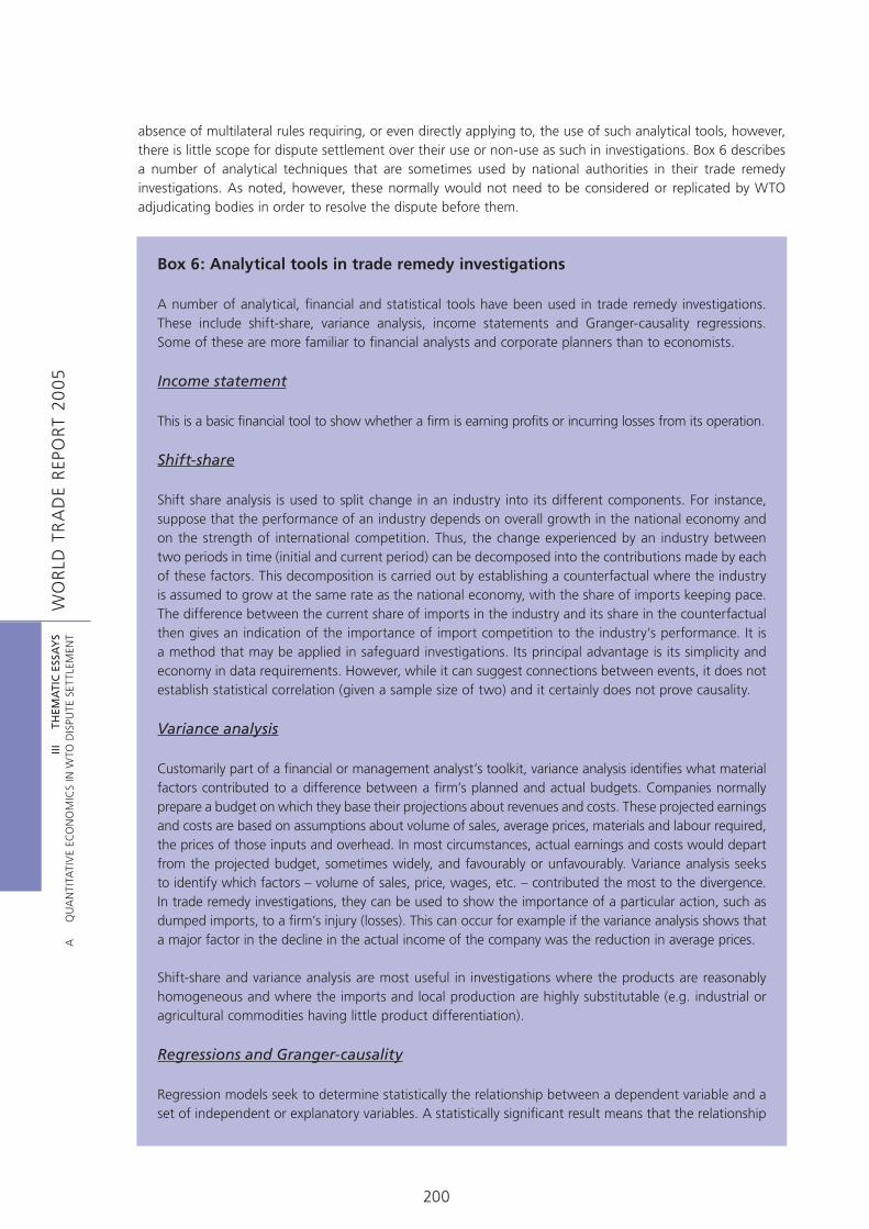
WO
RLD
TR
AD
E R
EPO
RT
200
5III
T
HEM
ATI
C E
SSA
YS
A
Q
UA
NTI
TATI
VE
ECO
NO
MIC
S IN
WTO
DIS
PUTE
SET
TLEM
ENT
200
absence of multilateral rules requiring, or even directly applying to, the use of such analytical tools, however, there is little scope for dispute settlement over their use or non-use as such in investigations. Box 6 describes a number of analytical techniques that are sometimes used by national authorities in their trade remedy investigations. As noted, however, these normally would not need to be considered or replicated by WTO adjudicating bodies in order to resolve the dispute before them.
Box 6: Analytical tools in trade remedy investigations
A number of analytical, financial and statistical tools have been used in trade remedy investigations. These include shift-share, variance analysis, income statements and Granger-causality regressions. Some of these are more familiar to financial analysts and corporate planners than to economists.
Income statement
This is a basic financial tool to show whether a firm is earning profits or incurring losses from its operation.
Shift-share
Shift share analysis is used to split change in an industry into its different components. For instance, suppose that the performance of an industry depends on overall growth in the national economy and on the strength of international competition. Thus, the change experienced by an industry between two periods in time (initial and current period) can be decomposed into the contributions made by each of these factors. This decomposition is carried out by establishing a counterfactual where the industry is assumed to grow at the same rate as the national economy, with the share of imports keeping pace. The difference between the current share of imports in the industry and its share in the counterfactual then gives an indication of the importance of import competition to the industry’s performance. It is a method that may be applied in safeguard investigations. Its principal advantage is its simplicity and economy in data requirements. However, while it can suggest connections between events, it does not establish statistical correlation (given a sample size of two) and it certainly does not prove causality.
Variance analysis
Customarily part of a financial or management analyst’s toolkit, variance analysis identifies what material factors contributed to a difference between a firm’s planned and actual budgets. Companies normally prepare a budget on which they base their projections about revenues and costs. These projected earnings and costs are based on assumptions about volume of sales, average prices, materials and labour required, the prices of those inputs and overhead. In most circumstances, actual earnings and costs would depart from the projected budget, sometimes widely, and favourably or unfavourably. Variance analysis seeks to identify which factors – volume of sales, price, wages, etc. – contributed the most to the divergence. In trade remedy investigations, they can be used to show the importance of a particular action, such as dumped imports, to a firm’s injury (losses). This can occur for example if the variance analysis shows that a major factor in the decline in the actual income of the company was the reduction in average prices.
Shift-share and variance analysis are most useful in investigations where the products are reasonably homogeneous and where the imports and local production are highly substitutable (e.g. industrial or agricultural commodities having little product differentiation).
Regressions and Granger-causality
Regression models seek to determine statistically the relationship between a dependent variable and a set of independent or explanatory variables. A statistically significant result means that the relationship

WO
RLD
TR
AD
E R
EPO
RT
200
5III
T
HEM
ATI
C E
SSA
YS
A
Q
UA
NTI
TATI
VE
ECO
NO
MIC
S IN
WTO
DIS
PUTE
SET
TLEM
ENT
201
between the dependent and the explanatory variables is not simply due to chance. The regression allows the user to know whether there is a positive, negative or no relationship between the explanatory and dependent variables. It also allows the user to quantify the relationship – how will a unit change in the independent variable affect the value of the dependent variable. It serves an important purpose in controlling for other factors that may have an influence on the dependent variable.
One specific regression model that is used in trade remedy investigations is the Granger-causality model. An economic variable x, say dumping, is said to Granger-cause another variable y, say losses to an industry, if past values of x provides information for predicting current and future values of y. In the context of a vector autoregression (VAR), which is the manner in which Granger-causality is carried out by economists, x is said to Granger-cause y if the addition of past values of x to a regression, involving a range of other explanatory variables to predict future values of y, results in an improvement in the prediction (e.g. a statistically significant reduction in the mean square error). It is important to note that this notion of causality is concerned with how information is sequenced in time and how useful it proves in prediction. For some, this may not agree with our ordinary understanding of what it means for one thing to cause another, although it is interesting to note the affinity with certain philosophical concepts of causality, e.g. Hume’s characterization of causality as constant conjunction rather than necessary connection. There is furthermore the question of whether Granger-causation alone will be sufficient evidence of a causal connection for an investigating authority.
An important use of this tool in trade remedy investigations in establishing whether dumping, subsidies or increased imports cause injury to domestic industry. Its principal strength is that it establishes a statistically significant correlation between two variables, say between prices for the goods at issue versus the world price of influential substitutes, which can be used to measure adverse domestic price effects attributable to the dumped goods versus other factors. The basic idea is that if the prices of competing, non-subject goods are accounting for most of the variations in domestic prices of the like product, then the residual variation arguably associated with the dumped goods may not be of material significance. Since the method requires time series data, observations must be available or sampled at regular intervals for it to be used since the reference period in trade remedy investigations is often relatively short. If one adopts a rule of thumb that at a bare minimum 30 (better, actually, 80 in times series analysis) observations (or more, particularly if there are long lags in the VAR) are necessary, then for Granger- causality to be used in a trade remedy investigation, the data must be available on a monthly or quarterly basis. Requiring data to be available on a weekly or fortnightly basis may be necessary in some but not all investigations.
Safeguards
The standard of review of safeguard investigations, which is the general standard of review applying to all WTO Agreements other than the Anti-Dumping Agreement, is given by Article 11 of the DSU. Article 11 charges the panel to “make an objective assessment of the matter before it, including an objective assessment of the facts of the case and the applicability of and conformity with the relevant covered agreements, and make such other findings as will assist the DSB in making the recommendations or in giving the rulings provided for in the covered agreements.”69 In the view of the Appellate Body, while this standard requires a panel to conduct a detailed examination of the substance of the investigation, such an examination does not constitute a de novo review (US–Lamb, Appellate Body Report: para. 106).
69 See also US–Lead Bars, Appellate Body Report: para. 45 on the appropriate standard of review for disputes under the SCM Agreement. Just what this means in practice has been clarified in a number of Appellate Body rulings, first with reference to Article 4.2 of the Safeguards Agreement and, subsequently, in regard to the entire Safeguards Agreement and obligations under GATT Article XIX. See US–Steel Safeguards, Appellate Body Report: para. 276.

WO
RLD
TR
AD
E R
EPO
RT
200
5III
T
HEM
ATI
C E
SSA
YS
A
Q
UA
NTI
TATI
VE
ECO
NO
MIC
S IN
WTO
DIS
PUTE
SET
TLEM
ENT
202
The Appellate Body has outlined a three-part test for how causation analysis, and in particular non-attribution analysis, should be conducted by authorities in safeguard investigations.70 While the Appellate Body has emphasized that there is no single methodology that must be used in conducting the causation analysis, panels and the Appellate Body in safeguard disputes examine whether the test has been properly applied by investigating authorities. First, the injury caused by increased imports is to be distinguished from the injury caused by “other factors”. Second, authorities must then attribute to increased imports, on the one hand, and to other relevant factors, on the other, the injury caused to domestic industry. As a final step, they must then determine whether the causal link exists between increased imports and serious injury, and whether this causal link involves a genuine and substantial relationship of cause and effect between these two elements (US–Wheat Gluten, Appellate Body Report: para. 69).71
In US–Line Pipe, for instance, the defendant (US) readily admitted that there was a decline in demand of line pipe that largely resulted from reduced oil and natural gas drilling and production activity and contributed to the serious injury experienced by the domestic industry. Yet, it did not consider the decline in oil and natural gas activities to be a greater contributing factor to the industry’s serious injury than the imports (US–Line Pipe, Panel Report: para. 7.288). This assertion was rejected by the panel (and, later, the Appellate Body). It noted that the injurious effects of the decline in the oil and gas industry were not separated from the ones due to increased imports. It was not enough to examine whether the relevant factor was a more important cause of serious injury than increased imports. In particular, the relative causal importance of the injurious effects of each other factor should be compared separately against the injurious effects of increased imports and not against the injury caused by increased imports and the remaining other factors together (US–Line Pipe, Panel Report: para. 7.289).
It is in connection to causation that in at least one dispute, parties have advanced, and the panel has considered, arguments in favour of the use of quantitative economics. In the US–Steel Safeguards dispute, in evaluating whether the investigating authorities had conducted a proper causation analysis, the panel addressed arguments by parties on the question of whether quantification is required and on the use of econometric models. The defendant (United States) had argued that the Agreement on Safeguards did not require quantification, and that quantification would be impossible to conduct. While the panel noted that the text of the Agreement on Safeguards did not require quantification it said that both the Agreement on Safeguards and relevant jurisprudence anticipated that quantification might occur.72 The exact form which quantification should take would depend upon the complexity of the situation under consideration. The more complex the situation, the more necessary a sophisticated analysis would become. Whatever approach or model was adopted, it should be applied in good faith and with due diligence.
In a different context (i.e. not in regard to causation analysis) of the US–Steel Safeguards case, a model was used by the US investigating authorities (the US International Trade Commission, USITC) prepared an economic model, similar to ones it had used over a long period of time (USTR, 2002b), as one element in the evaluation of remedy options under Article 5 of the Safeguards Agreement, i.e. in order to show that the safeguard measures were not applied beyond the extent necessary (US–Steel Safeguards, Panel Report: para. 7.1566, footnote 3619). With this model, the effects of trade remedies on supply and demand conditions and ultimately prices in the affected industry can be modelled, including through impacts of downstream and upstream industries. Again, results strongly depend on the values of the key parameters, namely the
70 The relevant provisions are contained in Article 4.2(b) of the Safeguard Agreement, which provides as follows: “The determination referred to in subparagraph (a) [on serious injury] shall not be made unless this investigation demonstrates, on the basis of objective evidence, the existence of the causal link between increased imports of the product concerned and serious injury or threat thereof. When factors other than increased imports are causing injury to the domestic industry at the same time, such injury shall not be attributed to increased imports.”
71 See also Argentina–Footwear (EC), Appellate Body Report: para. 144; US–Lamb, Appellate Body Report: paras. 178-181 and 185-186; US–Line Pipe, Appellate Body Report: paras 208, 215, 217 and 262; US–Steel Safeguards, Appellate Body Report: footnotes 494-495 to para. 481, paras. 483 and 489; and US–Wheat Gluten, Appellate Body Report: paras. 67-70.
72 The panel stated that “quantification may be particularly desirable in cases involving complicated factual situations where qualitative analyses may not suffice to more fully understand the dynamics of the relevant market ... [and that] the requirement in Article 4.2(a) that evaluated factors be of a ‘quantifiable nature’ implies that at least some of the factors assessed in the non-attribution exercise will be quantifiable and, in those circumstances, should be quantified” (US–Steel Safeguards, Panel Report: paras. 10.336-10.337). See also US–Steel Safeguards, Panel Report: paras. 10.340 and 10.707.

WO
RLD
TR
AD
E R
EPO
RT
200
5III
T
HEM
ATI
C E
SSA
YS
A
Q
UA
NTI
TATI
VE
ECO
NO
MIC
S IN
WTO
DIS
PUTE
SET
TLEM
ENT
203
Armington elasticity of substitution as well as the aggregate price elasticities of demand and supply of the domestic industry (USITC, 2002). Criticisms by complaining parties were levelled both at the fact that the model would result in an overestimation of the tariff required to restore the domestic industry to profitability and at the non-use of such a model in the causation and non-attribution analysis (US–Steel Safeguards, Panel Report: paras. 7.1649 ff). On the first issue, some of the simplifying assumptions of the model were attacked. It was noted, for instance, that treating imports and domestic production as “perfect substitutes” exaggerated the amount by which the average unit values of imports would need to be increased to put the industry in a state of non-injury (US–Steel Safeguards, Panel Report: para. 7.1663). In regard to the second assertion, parties referred to the abundance of data on which to base a quantification of the causes of injury to the domestic industry, on the use by the USITC economic staff of this type of model in earlier anti-dumping investigations and to the advantages of quantification, whenever other explanations seem counterintuitive (US–Steel Safeguards, Panel Report: para. 7.1527). For reasons of judicial economy, the panel ultimately did not need to consider claims under Article 5. But proceedings such as these illustrate that it cannot be excluded that panels may have to consider economic technicalities that parties challenge in each other’s argumentation.
Analytical techniques that may be relevant to causation in trade remedy cases
As noted above, although the applicable standards of review are different for anti-dumping disputes on the one hand and for countervailing duty and safeguards disputes on the other, the Appellate Body made it clear in US–Hot-Rolled Steel that the requirement to separate and distinguish the various factors causing injury, and their respective effects, which it first expressed in the context of safeguards, is not limited to that context. A number of commentators have considered the kinds of analytical techniques that might be relevant to the issues referred to in the three-part test.73
Although the Appellate Body’s three-part test seems straightforward, Sykes (2003) has critiqued WTO jurisprudence for not providing useful guidance on the causation issue.74 One criticism is that there is a tendency to equate correlation with causation. But a second and more fundamental criticism is that an analytical framework for establishing when imports cause serious injury to domestic industry is necessary because in many instances both are endogenous variables. In other words, both rising imports and injury to domestic injury can be the result of some other (third) factor. In these cases, although there is correlation between imports and injury, there is no causal link. These points can be clarified with diagrams depicting a simple demand and supply framework, as discussed by Irwin (2003) (see Box 7). For example, an increase in the cost of inputs to domestic production (which shifts the supply curve upward) can lead to both increased imports and lowered profitability and employment. But while there is a correlation between imports and injury, there is no causal connection, because, by assumption, the cause of the injury was a negative supply shock. In this analytical framework, imports can be a cause of injury when there is increased competition from foreign suppliers which shifts the supply of imports downward (to the right). Imports can also be a cause of injury if there is a reduction in tariffs, or in general, a relaxation of import barriers arising from a programme of trade liberalization. Authors like Irwin (2003) and Sykes (2003) highlight that the task of causation analysis is then to distinguish conceptually the latter case from those other instances when imports and injury are correlated but not causally linked.
73 Besides the relatively simple techniques presented in the following, some academics have also proposed more complex approaches, such as simultaneous equation models. See, in particular, Prusa and Sharp (2001); also Grossman (1986) and Pindyck and Rotemberg (1987).
74 As clarified above, there are certain areas where the WTO Agreements give discretion to the investigating authority as to the type of analysis that must be conducted and the type of methodology that has to be applied. The mandate of panels and the Appellate Body is to review determinations made by investigating authorities (including the analysis and methodologies used) for their consistency with the WTO Agreements.

WO
RLD
TR
AD
E R
EPO
RT
200
5III
T
HEM
ATI
C E
SSA
YS
A
Q
UA
NTI
TATI
VE
ECO
NO
MIC
S IN
WTO
DIS
PUTE
SET
TLEM
ENT
204
Box 7: A simple analytical framework on causation
The Charts below (based on Irwin, 2003: pp.28-29), show one simple approach to distinguish under what circumstances rising imports may be considered to “cause” injury to domestic industry and under what circumstances rising imports and injury to domestic industry may be by-products of some other cause. It is assumed that the importing country is small, i.e. unable to affect world price.
DD and SS are the domestic demand and supply of the product. WW is the world market price of imports. Initially, consumption is at OM, domestic production at OA and imports at AM. Suppose that there is a dramatic increase in the price of an input to this industry. The effect will be to shift the supply curve to the left (S’S’) leading to both lowered output (OC), employment and profits to the domestic industry as well as rising imports (CM). In this case there will be a correlation of rising imports and injury to the domestic industry, but it is clear that the trends are a consequence of a third factor (a domestic supply shock). So in this case, rising imports do not cause injury.
Now consider an improvement in the competitiveness of foreign suppliers which lowers the world market price from WW to W’W’. This leads to an increase in imports (M’M’) and a contraction in domestic output (to OA’), and in employment and profits. It is this second case, where rising imports may be seen as causing injury to domestic industry. Here an argument could be made that correlation implies causation.
Quantity
Price
MACO
W W
D
D
S
S‘
S‘
S
Price
AA‘ M M‘
W
W‘
W
W‘
O
D
D S
S
Quantity

WO
RLD
TR
AD
E R
EPO
RT
200
5III
T
HEM
ATI
C E
SSA
YS
A
Q
UA
NTI
TATI
VE
ECO
NO
MIC
S IN
WTO
DIS
PUTE
SET
TLEM
ENT
205
Irwin (2003) applied a tableau like the one in Table 3, which is based on such an analytical framework, to show what the predicted pattern of changes would be on domestic price, production, consumption and imports if (a) demand, or (b) supply or (c) imports is the initiating cause. Concretely, he looked at the predicted pattern of changes in four recent US safeguard investigations to see whether imports were indeed a causal factor in them. These cases were US–Wheat Gluten, US–Lamb, US–Line Pipe and US–Steel Safeguards. He finds that apart from US–Lamb, the other three cases suggested that imports were a causal factor.
Table 3Pattern of changes depending on cause
Cause Price Production Consumption Imports
Domestic demand increases No change No change ↑ ↑
Domestic supply reduction No change ↓ No change ↑
More import competition ↓ ↓ ↑ ↑
Note: Consistent with Box 7, it is assumed that the importing country is small – unable to change world prices.
Using also the basic demand supply framework of Box 7, Kelly (1988) has proposed a way of quantifying the impacts of demand shifts, domestic supply shifts and import competition to the domestic industry. The result is a decomposition of the reduction in domestic output (a proxy for the injury suffered by domestic industry) to the contribution made by demand changes, supply-side shocks and imports. The only additional pieces of information required for the quantification are elasticities of demand and supply. If the importing country is a large country, i.e. changes in imports have an impact on world price, and so faces an upward sloping import supply curve, then information on the import supply elasticity would be needed as well.
Kelly’s (1988) method seeks to produce numerical estimates of the contribution made by each factor and to provide an ordering of their relative importance. One possible problem with the Kelly (1988) method is that the apportionment it produces is quite broad or general – i.e. the contribution made by demand factors, supply-side factors and import competition. In actual safeguards investigations, investigating authorities look at more specific factors. For example, in the case of US–Lamb, the alternative cause of serious injury was the termination of government subsidies to lamb and sheep farmers.

WO
RLD
TR
AD
E R
EPO
RT
200
5III
T
HEM
ATI
C E
SSA
YS
A
Q
UA
NTI
TATI
VE
ECO
NO
MIC
S IN
WTO
DIS
PUTE
SET
TLEM
ENT
206
5. CONCLUSIONS
From the above discussion, especially of some of the arbitration cases, such as US–FSC (Article 22.6 – US) or US–Offset Act (Byrd Amendment) (EC) (Article 22.6 – US), a number of lessons may be drawn on how quantitative economic analysis can assist the dispute settlement process. First and foremost, where quantitative models were employed, they seem to have provided useful benchmark values against which qualitative outcomes could be checked. This is true despite the lack of absolute precision due to inherent difficulties in empirical work. For instance, a range of possible elasticity values may drive the modelling results, but still give a good impression of the direction and magnitude of trade effects and confirm a theoretical penchant or intuitive guess. Also on the positive side, quantitative economics need not be utterly complex. Comparative static partial equilibrium approaches seem sufficient in WTO dispute settlement, and general equilibrium considerations even out of place, since it is clear that “second-round” effects of a measure are not normally taken into account in the process of determining a breach of obligations or in arbitrating on the level of countermeasures.
The discussion of these arbitration cases, but also of, for example, Japan–Alcoholic Beverages II, Chile–Alcoholic Beverages or US–Upland Cotton suggests that if models are submitted, panels or arbitrators may feel compelled to consider a number of technical details. For example, which of two competing approaches is more adequate? What should the model specification be? What is the range of error introduced by sectoral aggregation? How good is the quality of data provided? How reliable are the results? While these questions call for the experience and technical skills of trade economists and econometricians, WTO dispute settlement is above all about determining well-reasoned outcomes on the basis of agreed legal texts. Empirical economic analysis rarely, if ever, can provide clear-cut answers. But, at a minimum, it can strengthen parties’ argumentation before panels and increase the comfort level of arbitrators in making an award.
Experience to date has confirmed that quantitative economic analysis cannot determine dispute settlement outcomes. Where quantitative analysis is used, it can certainly help to inform legal reasoning. Quantitative economics can help to avoid misinterpretation when economic rationality is counter-intuitive and less than obvious, although pertinent to the substance or direction of legal reasoning. But quantitative economic analysis will always play a supporting role to legal reasoning. As noted above, quantitative analysis is frequently beset by inherent methodological difficulties, the existence of competing approaches of apparently equal validity but that yield different results, simplifying assumptions and data limitations. Although analytical techniques and data will continue to improve, the supporting role of quantitative economics in dispute settlement will in our view remain essentially the same, even though these techniques may come to be used more intensively in the future.
All in all, there is a limited, but encouraging record of how quantitative economic analysis has been employed in dispute settlement proceedings. One reason why the use of quantitative economics may intensify in the future is that cases seem to become more and more “fact-intensive”. Parties are not subject to restrictions as to the type of evidence they wish to furnish, and panels themselves have often requested more detailed factual information. Hence, it is possible to discern a trend towards a higher level of technical sophistication upon which the legal argumentation is founded. Of course, this does not relate only to economic data and analysis. But, given the nature of WTO Agreements, market competition and trade impacts are usually at issue, and in the context of certain legal provisions, quantitative economic analysis may be called for in the future, where so far this has not been so. If understood as a complementary tool to acquire better insights into the effects of policies on trade or of imports in the domestic market, there is no reason to believe that economic analysis could not make a bigger contribution to an effective functioning of the dispute settlement process.
WO
RLD
TR
AD
E R
EPO
RT
200
5III
T
HEM
ATI
C E
SSA
YS
A
Q
UA
NTI
TATI
VE
ECO
NO
MIC
S IN
WTO
DIS
PUTE
SET
TLEM
ENT
207
BIBLIOGRAPHY
Anderson, K. (2002) ‘Peculiarities of retaliation in the WTO dispute settlement’, World Trade Review 1, 2: 123-134.
Anderson, S. (2004) ‘Meeting the Burden of Proof – A Practitioner’s Guide to Documents, Witnesses, Experts and Adverse Inferences’, paper presented at the Seventh Annual Conference on Dispute Resolution in the WTO, organized by Cameron May, 18 June 2004, Geneva.
Armington, J. S. (1969) ‘A theory of demand for products distinguished by place of production’, IMF Staff Papers 16: 159-177.
Babcock, B. A., Beghin, J. C., Fabiosa, J. F., De Cara, S., Elobeid, A., Fang, C., Hart, C. E., Isik, M., Matthey, H., Saak, A. E., Kovarik K. and FAPRI Staff (2002) ‘The Doha Round of the World Trade Organization: Appraising Further Liberalization of Agricultural Markets’, Food and Agricultural Policy Research Institute (FAPRI) Working Paper 02-WP 317. Available online http://www.fapri.org/publications/wto.aspx. Accessed 03/03/05.
Bagwell, K. and Staiger, R. (2002) The Economics of the World Trading System, Cambridge, MA: MIT Press.
Bernstein, J. and Skully, D. (2003) ‘Calculating Trade Damages in the Context of the World Trade Organisation’s Dispute Settlement Process’, Review of Agricultural Economics 25, 2: 385-398.
Bown, C. P. (2002) ‘The Economics of Trade Disputes, the GATT’s Article XXIII, and the WTO’s Dispute Settlement Understanding’, Economics and Politics 14, 3: 283-323.
Breuss, F. (2004) ‘WTO Dispute Settlement: An Economic Analysis of Four EU-US Mine Trade Wars’, Journal of Industry, Competition and Trade 4, 4: 275-315.
Busch, M. L. and Reinhardt, E. (2003) ‘Developing Countries and GATT/WTO Dispute Settlement’, mimeo.
Butler, M. and Hauser, H. (2000) ‘The WTO Dispute Settlement Mechanism: A First Assessment from an Economic Perspective’, Journal of Law, Economics and Organization 16, 2: 503-533.
Donnelly, W. A., Johnson, K. Tsigas, M. and Ingersoll, D. (2004) ‘Revised Armington Elasticities of Substitution for the USITC Model and the Concordance for Constructing a Consistent Set for the GTAP Model’, Office of Economics Research Note, U.S. International Trade Commission (USITC), Washington: USITC.
Francois, J. F. and Hall, H.K (2003) ‘Global Simulation Analysis of Industry-Level Trade Policy’, Version 3.0: 21 April 2003, mimeo.
Francois, J. F. and Reinert, K. A. (1997) ‘Applied Methods for Trade Policy Analysis: An Overview’, in: Francois, J. F. and Reinert, K. (eds.) Applied Methods for Trade Policy Analysis: A Handbook, Cambridge: Cambridge University Press: 3-24.
Gasmi, F., Laffont J.-J. and Vuong, Q. (1992) ‘Econometric Analysis of Collusive Behavior in a Soft Drink Market’, Journal of Economics and Management Strategy 1: 278-311.
Grossman, G. M. (1986) ‘Imports as a Cause of Injury: The Case of the U.S. Steel Industry’, Journal of International Economics 20: 201-223.
Harvey, A. C. (1990) The Econometric Analysis of Time Series, second edition, Cambridge, MA: MIT Press.
Hertel, T. W. (1990) ‘General Equilibrium Analysis of U.S. Agriculture: What Does It Contribute?’, The Journal of Agricultural Economics Research 42, 3: 3-9.
Hertel, T. W., Lanclos, D. K., Pearson, K. R. and Swaminathan, P. V. (1997) ‘Aggregation and computation of equilibrium elasticities’, in: Hertel, T. W. (ed.) Global Trade Analysis: Modeling and Applications, Cambridge: Cambridge University Press: 149-163.
Horn, H. and Mavroidis, P. C. (eds.) (2003) The WTO Case Law of 2001, The American Law Institute Reporters’ Studies, Cambridge: Cambridge University Press.
– (2004) ‘Still Hazy after All These Years: The Interpretation of National Treatment in the GATT/WTO Case-Law on Tax Discrimination’, European Journal of International Law 15, 1: 39-69.

WO
RLD
TR
AD
E R
EPO
RT
200
5III
T
HEM
ATI
C E
SSA
YS
A
Q
UA
NTI
TATI
VE
ECO
NO
MIC
S IN
WTO
DIS
PUTE
SET
TLEM
ENT
208
Horn, H., Nordström, H. and Mavroidis, P. C. (1999) ‘Is the Use of the WTO Dispute Settlement System Biased?’, CEPR Discussion Paper 2340, London: Centre for Economic Policy Research.
Houthakker, H. S. and Magee, S. P. (1969) ‘Income and Price Elasticities in World Trade’, Review of Economics and Statistics 51, 2: 111-125.
Huff, K. M., Hanslow, K., Hertel, T. W. and Tsigas, M. E. (1997) ‘GTAP behavioural parameters’, in: Hertel, T. W. (ed.) Global Trade Analysis: Modeling and Applications, Cambridge: Cambridge University Press: 124-148.
Irwin, D. A. (2003) ‘Causing Problems? The WTO Review of Causation and Injury Attribution in US Section 201 Cases’, World Trade Review 2, 3: 297-325.
Keck, A. (2004) ‘WTO Dispute Settlement: What Role for Economic Analysis?’, Journal of Industry, Competition and Trade 4, 4: 365-371.
Kee, H. L., Nicita A. and Olarreaga, M. (2004) ‘Import Demand Elasticities and Trade Distortions’, World Bank Research Working Paper No. 3452, Washington: World Bank.
Keller, W. J. (1980) Tax incidence: A General Equilibrium Approach, Amsterdam: North Holland Press.
Kelly, K. (1988) ‘The Analysis of Causality in Escape Clause Cases’, Journal of Industrial Economics, 37: 187–207.
Kennedy, P. (1987) A Guide to Econometrics, second edition, Cambridge, MA.: MIT Press.
Lawrence, R. Z. (2003) Crimes and Punishment: Retaliation under the WTO, Washington, DC: Institute for International Economics (IIE).
Leitner, K. and Lester, S. (2003) ‘WTO Dispute Settlement 1995-2002: A Statistical Analysis’, Journal of International Economic Law (JIEL) 6, 1: 251-261.
Maggi, G. (1999) ‘The Role of Multilateral Institutions in International Trade Co-operation’, American Economic Review 89, 1: 190-214.
Malashevich, B. (2004) ‘The Metrics of Economics As Applied to WTO Dispute Settlement’, presentation made at the Seventh Annual Conference on Dispute Resolution in the WTO, organized by Cameron May, 18 June 2004, Geneva.
Marquez, J. (1990) ‘Bilateral Trade Elasticities’, Review of Economics and Statistics 72, 1: 70-77.
– (1999) ‘Long-Period Trade Elasticities for Canada, Japan and the United States’, Review of International Economics 7, 1: 102-116.
McDaniel, C. A. and Balistreri, E. J. (2002) ‘A Discussion of Armington Trade Substitution Elasticities’, Office of Economics Working Paper, US International Trade Commission (USITC), Washington: USITC.
Neven, D. (2000) ‘Evaluating the effects of non tariff barriers: The economic analysis of protection in WTO disputes’, mimeo.
Pindyck, R. S. and Rotemberg, J. J. (1987) ‘Are Imports to Blame? Attribution of Injury under the 1974 Trade Act’, Journal of Law and Economics 30: 101-122.
Prusa, T. J. and Sharp, D. C. (2001) ‘Simultaneous Equations in Antidumping Investigations’, Journal of Forensic Economics 14: 63-78.
Stern, R. M. (1973) The Balance of Payments, Chicago: Aldine.
Stern, R. M., Francis, J. and Schumacher, B. (1976) Price Elasticities in International Trade: An Annotated Bibliography, Trade Policy Research Centre, London: The Macmillan Press.
Sumner, D. A., Barichello, R. C. and Paggi, M. S. (2003) ‘Economic Analysis in Disputes of Trade Remedy and Related Measures in Agriculture, with Examples from Recent Cases’, Paper presented at the International Conference “Agricultural policy reform and the WTO: where are we heading?”, 23-26 June 2003, Capri.
Sykes, A. O. (2003) ‘The Safeguards Mess: A Critique of WTO Jurisprudence’, World Trade Review 2, 3: 261-295.

WO
RLD
TR
AD
E R
EPO
RT
200
5III
T
HEM
ATI
C E
SSA
YS
A
Q
UA
NTI
TATI
VE
ECO
NO
MIC
S IN
WTO
DIS
PUTE
SET
TLEM
ENT
209
United States International Trade Commission (USITC) (2002) ‘Available information on economic models (public version)’, mimeo. Available online http://www.usitc.gov. Accessed 03/03/05.
United States Trade Representative (USTR) (2002a) ‘United States - Tax Treatment for “Foreign Sales Corporations” - Recourse by the United States to Article 22.6 of the DSU and Article 4.11 of the SCM Agreement, Second Written Submission of the United States of America, February 26, 2002’, mimeo. Available online http://www.ustr.gov. Accessed 03/03/05.
– (2002b) ‘United States - Definitive Safeguard Measures on Imports of Certain Steel Products, First Written Submission of the United States of America, October 4, 2002’, mimeo. Available online http://www.ustr.gov. Accessed 03/03/05.
Varian, H. R. (1984) Microeconomic analysis, second edition, New York & London: W. W. Norton & Company.
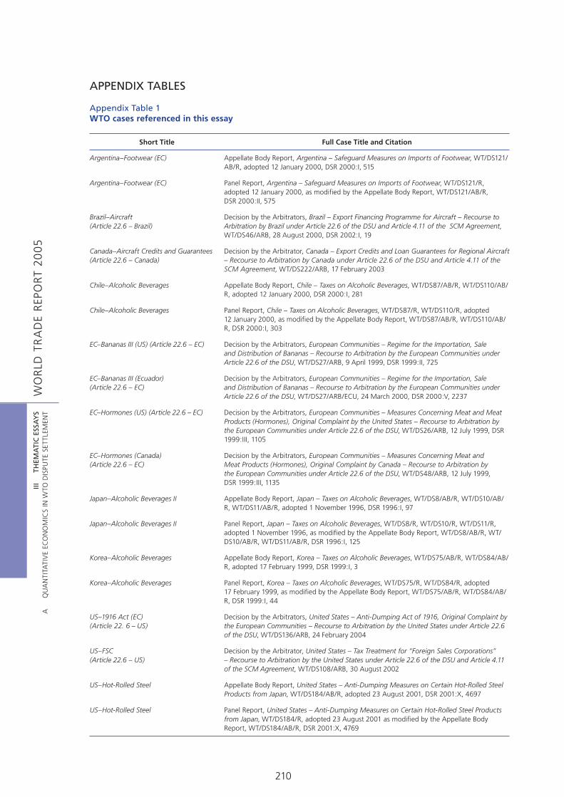
WO
RLD
TR
AD
E R
EPO
RT
200
5III
T
HEM
ATI
C E
SSA
YS
A
Q
UA
NTI
TATI
VE
ECO
NO
MIC
S IN
WTO
DIS
PUTE
SET
TLEM
ENT
210
APPENDIX TABLES
Appendix Table 1WTO cases referenced in this essay
Short Title Full Case Title and Citation
Argentina–Footwear (EC) Appellate Body Report, Argentina – Safeguard Measures on Imports of Footwear, WT/DS121/AB/R, adopted 12 January 2000, DSR 2000:I, 515
Argentina–Footwear (EC) Panel Report, Argentina – Safeguard Measures on Imports of Footwear, WT/DS121/R, adopted 12 January 2000, as modified by the Appellate Body Report, WT/DS121/AB/R, DSR 2000:II, 575
Brazil–Aircraft (Article 22.6 – Brazil)
Decision by the Arbitrators, Brazil – Export Financing Programme for Aircraft – Recourse to Arbitration by Brazil under Article 22.6 of the DSU and Article 4.11 of the SCM Agreement, WT/DS46/ARB, 28 August 2000, DSR 2002:I, 19
Canada–Aircraft Credits and Guarantees (Article 22.6 – Canada)
Decision by the Arbitrator, Canada – Export Credits and Loan Guarantees for Regional Aircraft – Recourse to Arbitration by Canada under Article 22.6 of the DSU and Article 4.11 of the SCM Agreement, WT/DS222/ARB, 17 February 2003
Chile–Alcoholic Beverages Appellate Body Report, Chile – Taxes on Alcoholic Beverages, WT/DS87/AB/R, WT/DS110/AB/R, adopted 12 January 2000, DSR 2000:I, 281
Chile–Alcoholic Beverages Panel Report, Chile – Taxes on Alcoholic Beverages, WT/DS87/R, WT/DS110/R, adopted 12 January 2000, as modified by the Appellate Body Report, WT/DS87/AB/R, WT/DS110/AB/R, DSR 2000:I, 303
EC–Bananas III (US) (Article 22.6 – EC) Decision by the Arbitrators, European Communities – Regime for the Importation, Sale and Distribution of Bananas – Recourse to Arbitration by the European Communities under Article 22.6 of the DSU, WT/DS27/ARB, 9 April 1999, DSR 1999:II, 725
EC–Bananas III (Ecuador) (Article 22.6 – EC)
Decision by the Arbitrators, European Communities – Regime for the Importation, Sale and Distribution of Bananas – Recourse to Arbitration by the European Communities under Article 22.6 of the DSU, WT/DS27/ARB/ECU, 24 March 2000, DSR 2000:V, 2237
EC–Hormones (US) (Article 22.6 – EC) Decision by the Arbitrators, European Communities – Measures Concerning Meat and Meat Products (Hormones), Original Complaint by the United States – Recourse to Arbitration by the European Communities under Article 22.6 of the DSU, WT/DS26/ARB, 12 July 1999, DSR 1999:III, 1105
EC–Hormones (Canada) (Article 22.6 – EC)
Decision by the Arbitrators, European Communities – Measures Concerning Meat and Meat Products (Hormones), Original Complaint by Canada – Recourse to Arbitration by the European Communities under Article 22.6 of the DSU, WT/DS48/ARB, 12 July 1999, DSR 1999:III, 1135
Japan–Alcoholic Beverages II Appellate Body Report, Japan – Taxes on Alcoholic Beverages, WT/DS8/AB/R, WT/DS10/AB/R, WT/DS11/AB/R, adopted 1 November 1996, DSR 1996:I, 97
Japan–Alcoholic Beverages II Panel Report, Japan – Taxes on Alcoholic Beverages, WT/DS8/R, WT/DS10/R, WT/DS11/R, adopted 1 November 1996, as modified by the Appellate Body Report, WT/DS8/AB/R, WT/DS10/AB/R, WT/DS11/AB/R, DSR 1996:I, 125
Korea–Alcoholic Beverages Appellate Body Report, Korea – Taxes on Alcoholic Beverages, WT/DS75/AB/R, WT/DS84/AB/R, adopted 17 February 1999, DSR 1999:I, 3
Korea–Alcoholic Beverages Panel Report, Korea – Taxes on Alcoholic Beverages, WT/DS75/R, WT/DS84/R, adopted 17 February 1999, as modified by the Appellate Body Report, WT/DS75/AB/R, WT/DS84/AB/R, DSR 1999:I, 44
US–1916 Act (EC)
(Article 22. 6 – US)Decision by the Arbitrators, United States – Anti-Dumping Act of 1916, Original Complaint by the European Communities – Recourse to Arbitration by the United States under Article 22.6 of the DSU, WT/DS136/ARB, 24 February 2004
US–FSC (Article 22.6 – US)
Decision by the Arbitrator, United States – Tax Treatment for “Foreign Sales Corporations” – Recourse to Arbitration by the United States under Article 22.6 of the DSU and Article 4.11 of the SCM Agreement, WT/DS108/ARB, 30 August 2002
US–Hot-Rolled Steel Appellate Body Report, United States – Anti-Dumping Measures on Certain Hot-Rolled Steel Products from Japan, WT/DS184/AB/R, adopted 23 August 2001, DSR 2001:X, 4697
US–Hot-Rolled Steel Panel Report, United States – Anti-Dumping Measures on Certain Hot-Rolled Steel Products from Japan, WT/DS184/R, adopted 23 August 2001 as modified by the Appellate Body Report, WT/DS184/AB/R, DSR 2001:X, 4769

WO
RLD
TR
AD
E R
EPO
RT
200
5III
T
HEM
ATI
C E
SSA
YS
A
Q
UA
NTI
TATI
VE
ECO
NO
MIC
S IN
WTO
DIS
PUTE
SET
TLEM
ENT
211
Short Title Full Case Title and Citation
US–Lamb Appellate Body Report, United States – Safeguard Measures on Imports of Fresh, Chilled or Frozen Lamb Meat from New Zealand and Australia, WT/DS177/AB/R, WT/DS178/AB/R, adopted 16 May 2001, DSR 2001:IX, 4051
US–Lamb Panel Report, United States – Safeguard Measures on Imports of Fresh, Chilled or Frozen Lamb Meat from New Zealand and Australia, WT/DS177/R, WT/DS178/R, adopted 16 May 2001, as modified by the Appellate Body Report, WT/DS177/AB/R, WT/DS178/AB/R, DSR 2001:IX, 4107
US–Line Pipe Appellate Body Report, United States – Definitive Safeguard Measures on Imports of Circular Welded Carbon Quality Line Pipe from Korea, WT/DS202/AB/R, adopted 8 March 2002
US–Line Pipe Panel Report, United States – Definitive Safeguard Measures on Imports of Circular Welded Carbon Quality Line Pipe from Korea, WT/DS202/R, adopted 8 March 2002, as modified by the Appellate Body Report, WT/DS202/AB/R
US–Offset Act (Byrd Amendment) (Brazil) (Article 22.6 – US)
Decision by the Arbitrator, United States – Continued Dumping and Subsidy Offset Act of 2000, Original Complaint by Brazil – Recourse to Arbitration by the United States under Article 22.6 of the DSU, WT/DS217/ARB/BRA, 31 August 2004
US–Offset Act (Byrd Amendment) (Canada) (Article 22.6 – US)
Decision by the Arbitrator, United States – Continued Dumping and Subsidy Offset Act of 2000, Original Complaint by Canada – Recourse to Arbitration by the United States under Article 22.6 of the DSU, WT/DS234/ARB/CAN, 31 August 2004
US–Offset Act (Byrd Amendment) (Chile) (Article 22.6 – US)
Decision by the Arbitrator, United States – Continued Dumping and Subsidy Offset Act of 2000, Original Complaint by Chile – Recourse to Arbitration by the United States under Article 22.6 of the DSU, WT/DS217/ARB/CHL, 31 August 2004
US–Offset Act (Byrd Amendment) (EC)(Article 22.6 – US)
Decision by the Arbitrator, United States – Continued Dumping and Subsidy Offset Act of 2000, Original Complaint by the European Communities – Recourse to Arbitration by the United States under Article 22.6 of the DSU, WT/DS217/ARB/EEC, 31 August 2004
US–Offset Act (Byrd Amendment) (India)(Article 22.6 – US)
Decision by the Arbitrator, United States – Continued Dumping and Subsidy Offset Act of 2000, Original Complaint by India – Recourse to Arbitration by the United States under Article 22.6 of the DSU, WT/DS217/ARB/IND, 31 August 2004
US–Offset Act (Byrd Amendment) (Japan)(Article 22.6 – US)
Decision by the Arbitrator, United States – Continued Dumping and Subsidy Offset Act of 2000, Original Complaint by Japan – Recourse to Arbitration by the United States under Article 22.6 of the DSU, WT/DS217/ARB/JPN, 31 August 2004
US–Offset Act (Byrd Amendment) (Korea)(Article 22.6 – US)
Decision by the Arbitrator, United States – Continued Dumping and Subsidy Offset Act of 2000, Original Complaint by Korea – Recourse to Arbitration by the United States under Article 22.6 of the DSU, WT/DS217/ARB/KOR, 31 August 2004
US–Offset Act (Byrd Amendment) (Mexico) (Article 22.6 – US)
Decision by the Arbitrator, United States – Continued Dumping and Subsidy Offset Act of 2000, Original Complaint by Mexico – Recourse to Arbitration by the United States under Article 22.6 of the DSU, WT/DS234/ARB/MEX, 31 August 2004
US–Steel Safeguards Appellate Body Report, United States – Definitive Safeguard Measures on Imports of Certain Steel Products, WT/DS248AB/R, WT/DS249AB/R, WT/DS251AB/R, WT/DS252AB/R, WT/DS253AB/R, WT/DS254AB/R, WT/DS258AB/R, WT/DS259AB/R, adopted 10 December 2003
US–Steel Safeguards Panel Report, United States – Definitive Safeguard Measures on Imports of Certain Steel Products, WT/DS248, WT/DS249, WT/DS251, WT/DS252, WT/DS253, WT/DS254, WT/DS258, WT/DS259, adopted 10 December 2003, as modified by the Appellate Body Report, WT/DS248AB/R, WT/DS249AB/R, WT/DS251AB/R, WT/DS252AB/R, WT/DS253AB/R, WT/DS254AB/R, WT/DS258AB/R, WT/DS259AB/R
US–Upland Cotton Panel Report, United States – Subsidies on Upland Cotton, WT/DS267/R, and Corr.1, 8 September 2004
US–Upland Cotton Appellate Body Report, United States – Subsidies on Upland Cotton, WT/DS267/AB/R, 3 March 2005
US–Wheat Gluten Appellate Body Report, United States – Definitive Safeguard Measures on Imports of Wheat Gluten from the European Communities, WT/DS166/AB/R, adopted 19 January 2001, DSR 2001:II, 717
US–Wheat Gluten Panel Report, United States – Definitive Safeguard Measures on Imports of Wheat Gluten from the European Communities, WT/DS166/R, adopted 19 January 2001, as modified by the Appellate Body Report, WT/DS166/AB/R, DSR 2001:III, 779