i

Igpet for Mac Copyright January 9, 2000

Terra Softa Inc. 155 Emerson Rd.

Somerset, NJ 08873

Phone/Fax: 732-937-4596 email: carrvolcano@gmail.com

https://sites.google.com/site/igpethome/home

Version: 24 February 2017

ii

I do this in my spare time so debugging is inadequate. I will send out repairs if needed. Please report any difficulties. If I can reproduce a flaw, I can fix it.

Upgrade Notes 24 February 2017 Changed file structure to make Igpet work in OSX Sierra. Code Signing was added in December, so installation on Sierra should be OK. 6 January 2017 Changed “Scale to Variable” to adjust sizes of symbols 29 December 2016 Modified PDF setup, added Installation help 6 April 2016 Improved Spider modeling by calculating and displaying the maximum % of melting for non-modal melting. Made PageMax automatic if Position is anything other than default. 15 March 2015 Changing colors in the Symbols page resulted in new colors on the screen but the new colors were not carried over to the PDF version, which is the only version that can be saved. At least the repair was easy. Nov 25, 2015 Many small improvements based on experience in creating the Igpet Work-book. Clarified the use of several Diagram files: IrvineBaragar.txt, DiscrimBasalt.txt and RockType.txt. Posted Igpet Workbook to homepage. Created a Teaching version of Igpet. Sept 23, 2015 Fixed missing isotope calcs for spider mixing, (Pb isos) August 24 2015 Added new PC file from Laubier et al. 2014. Added Tormey et al. (1987) and Grove et al. (2003) and improved other CMAS projections from Grove’s research group. August 21 2015 Once again repaired Igpet’s ability to read data files in formats other than US English. Nthfield() was adding quote marks if a , was the decimal marker. May 16 2015 Minor change in calculation of eNdo in extra.txt. Made the value of CHUR visi-ble and added a o subscript to indicate that this is a zero age calculation. Jan 22,24 2015 Repaired flaw in trace element calculation in Mixing. Flaw was introduced in December. In Igpet, made the launch of Preview optional when saving a diagram. Jan 12 2015 Adobe Illustrator was translating the x-axis numbers into a continuous string, making it awkward to edit in Ai. Fixed this by adding dummy print commands. Now each label is discrete. Fixed in XY, Spider and Histogram plots. Dec 10-14 2014 Added ability to draw double triangles “DTRI” for IUGS rock classification and allowed small fonts in PDF Diagrams. Simplified the calculation of normalized element values Eu* etc. Changed output logic for Mixing, CIPW and PTfO2. Fixed a bug in Igpet’s ‘add a file’ logic.

iii

Nov 20, 2014 Added logic that allows a Legend to be plotted for a histogram. Made major internal changes to file handling and plotting of characters on the screen. These changes were required to accommodate the phasing out of useful functions in the XoJo programing language. They “should” be invisible to users. Rewrote and simplified the isotopic mixing in SpiMix using DePaolo equations. This allows mixing for epsilon Nd and epsilon Sr. Removed a glitch for mixing and modeling Pb isotopes in spiderplots. Created a Teaching version of Igpet that writes jpeg files. June 30, 2014 Added polynomial regression to XY plots Feb 8, 2014 Repaired a bug in File Operations-Add a file Nov 24, 2013 Created a utility to partition Fe3 and Fe2 using Beattie (1993) and Kress and Carmichael (1991). Incorporated this logic into Igpet for CMAS and Pearce calculations, re-placing the Sack et al (1980) logic that used just one T and fO2 Nov 10, 2013 Created a Zoom button to blow up a portion of an XY plot. It is a crude zoom that needs to be adjusted with an Axis call. Created decent Mineral plots for Feldspars and the PX quad. Made the min-eral keys the same on all PC files added another special keyword, “Mineral” to identify the minerals in mineral data files, e.g. ol is olivine. Significant changes in Mixing program and Mineral Plots to use this new keyword. Aug 22, 2013 Added Hoffman (2007) Mantle isotopic diagrams Aug 4-8, 2013 Added ability to read csv (comma delimited) files and the ability to convert many GEOROC column headings (variable names) to Igpet friendly names. Made the file read method identify the first occurrence of “samp” in the top row as the column of sample names. Made several other small improvements. June 13, 2013 Major upgrade to vector graphics as PDF function is added. No doubt many bugs are crawling about but still a huge improvement in output quality June 6, 2013 Refixed the Axis bug of March 25 and extended the fix to other areas that use inputfrm. May 29, 2013 Changes some logic in Spider plots to allow spaces to be ignored in element labels in spider.txt March 25 2013 Fixed Axis bug introduced by REALbasic change Feb 21, 2013 Fixed flaw in Lindsley Anderson px geothermometer, now correct again. Jan 3, 2013 Fixed flaw in mixing if the variable was [N] normalized (S-Norm function)

iv

Oct 2, 2012 substantial improvement of REE Inverse modeling Aug 29, 2012 Added mixing and recharge models to Spider modeling. Made new PC files. Added Mantle_traces data file. Aug 15, 2012 Cleaned up some issues in XY Models. Improved the Variable form Aug 7, 2012 Added ability to use epsilon Nd and epsilon Sr in AFC models in Spider plots. May 16, 2012 Fixed various flaws in histogram, principally concerning Log values. Added logic to allow user to change the suggested % melts for Spider modeling. File PercentFs.txt holds the strings of melt %s . Apr 19, 2012 Found and fixed a serious flaw in the AFC calculations for isotopes in the Spi-der modeling section. Oct 16, 2011 Added a legend that writes a separate diagram, just a legend. Dec 17, 2010 Fixed a flaw in Equilib. Xtall. Calculation in spider modeling. Made changes to Histogram but still have some uncertainty about the correctness, so I will revisit it. Aug 31 2010 Minor changes to ferrous ferric ratio adjustment Jan 2010 Improvement to CoDoPi, REE inverse modeling. Aug 26, 2009 Series of significant changes. Added more diagrams and the Peacock index. Improved transfer of drawings from Igpet to Word and Powerpoint. Made significant im-provement to handling of isotopic data. Added Hf and Os into AFC modeling. The Model sec-tion of Spiderplots now does AFC calculations for isotopes as well as trace elements. March 2008 Significant upgrade. Added logic for Hf and Os isotopes. Added AFM calcs for isotopes (Sr, Nd, Hf, Os, Pb) in the spiderplot modeling section. Added Isotope mixing in the Spider Mixing section. Improved screen logic to better handle screens that do not have a 4/3 aspect ratio. Fixed error bars for log plots, bug in Diagram printing, added a few new diagrams August 2007 Added AFC models to the modeling in the spiderplots December 2006 Major programming changes that should not affect user. Large change in Folder structure (essentially creating a folder structure) 2005 Improved the Legend and added/repaired many diagrams. Added a text box to calcu-lator. Added a Legend and many smaller improvements and repairs

v

2004 Major upgrade. Significant change in programming environment, serious attempt to fix international problems involving erroneous truncation of numbers after local decimal characters that are not a “.” but are instead a “,”.

Acknowledgments My wife and son put up with a lot, allowing me to work on this. My colleagues and semi-willing beta testers, Mark Feigenson, Claude Herzberg, Lina Patino, Karen Bemis, Esteban Gazel, Fara Lindsay and many others repeatedly demonstrate uncanny ability to locate bugs within minutes of getting a "final" version. Over the years several geoscientists have found bugs for me and suggested or provided useful additions. This is a major way that Igpet im-proves.

vi

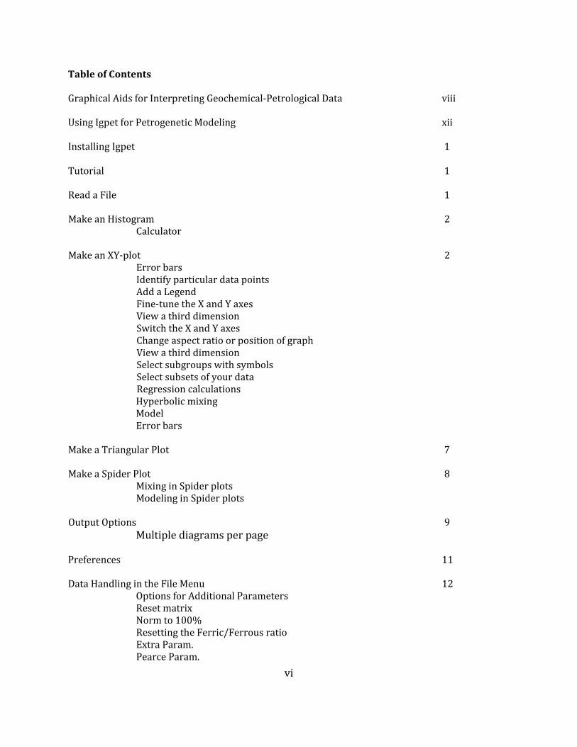
Table of Contents Graphical Aids for Interpreting Geochemical-Petrological Data viii Using Igpet for Petrogenetic Modeling xii Installing Igpet 1 Tutorial 1 Read a File 1 Make an Histogram 2 Calculator Make an XY-plot 2 Error bars Identify particular data points Add a Legend Fine-tune the X and Y axes View a third dimension Switch the X and Y axes Change aspect ratio or position of graph View a third dimension Select subgroups with symbols Select subsets of your data Regression calculations Hyperbolic mixing Model Error bars Make a Triangular Plot 7 Make a Spider Plot 8 Mixing in Spider plots Modeling in Spider plots Output Options 9 Multiple diagrams per page Preferences 11 Data Handling in the File Menu 12 Options for Additional Parameters Reset matrix Norm to 100% Resetting the Ferric/Ferrous ratio Extra Param. Pearce Param.

vii

CIPW Norms Rock and Mineral Data Files 16 Tab delimited file structure Comma delimited data file structure Format features Using Igpet's File Operations 17 View data Save file Add a file (Merge Files) Read the Clipboard Pre-designed Diagrams 18 Mineral diagrams CMAS projections Special Diagrams Discrimination and classification diagrams Spider diagrams Notes on some calculations 20 Mixing and Mixing AFC Modeling Adding tie lines Common Problems 21 Zeros are not plotted Errors in the data file Mixing.app 22 PTfO2.app 24 Appendix A: Control Files 25 Appendix B: Data files 36 Appendix C: References 38 Appendix D: IUGS diagrams 48

viii

Graphical Aids for Interpreting Geochemical-Petrological Data: Peaks & Pitfalls

Igpet and Mixing can display data beautifully and make a variety of complicated calculations, but rarely do these tools prove anything! What these programs can most reliably do is prove hypotheses incorrect. Usually, after considerable effort, one can find a version of a hypothe-sis, such as fractional crystallization, that is consistent with available evidence, not that it is proved. All too often this inherent limitation is forgotten and weak hypotheses are deemed correct on flimsy graphical evidence. In my experience the worst pitfall of this software is the ease with which fuzzy thinking is translated into attractive diagrams that are pasted into papers and theses without much useful thought. I am intimately familiar with some varieties of misbegotten interpretations because I have done them myself! The paragraphs below summarize some of the false paths Igpet can lead a student down as well as some helpful approaches. The correct approach to solving the problem of how a suite of samples of igneous rocks might be related to each other is first to look at the hand samples and thin sections of all (or at least half!) of the samples. The thin sections can immediately set the tone for the problem at hand. Assuming the samples are all from the same volcano or from a group of geographically and temporally associated vents, one can start wondering about how they are related. My pre-ferred sample set is a long stratigraphic sequence from a caldera wall. Nature is rarely so co-operative. If the samples are aphyric, or nearly so, there is a reasonable chance you may be examining a set of separate melts, so some type of partial melting hypothesis can be consid-ered. If a plot of MgO versus K2O is a mess, with a large K2O range and little or no consistent potash increase as MgO decreases, then you should get more incompatible element data, es-pecially REE data, in order to test various partial melting models. If, instead, there is a strong inverse relationship between potash and magnesia, then fractional crystallization becomes the first hypothesis to test. The presence of abundant phenocrysts and, especially, the presence of disequilibrium tex-tures and assemblages should make one worry about mixing and accumulation processes. If olivines and quartz are in the same thin section, then something is wrong! Either mixing or assimilation is likely except in the rare cases of some Fe rich granophyres with fayalite and quartz. Electron microprobe analyses of minerals (olivines, plagioclase, clinopyroxene, etc) that define two distinct populations (a bimodal distribution) are fairly definitive evidence for magma mixing that has occurred too recently for the phenocryst evidence to be swept away by the thermodynamic drive toward equilibrium in a large magma chamber. Igpet is a tool but not a textbook. There are several useful petrology and geochemistry books. The more elegant calculations in Igpet either came from Albarede’s 1995 book, Introduction to Geochemical Modeling, or are reproduced there. The reference list at the end of this man-ual is included to be USED, especially, some rather old references: e,g. O'Hara (1968 and 1976) for CMAS projections; Bryan, Finger and Chayes (1968) for petrologic mixing calcula-tions; Chayes (1964) on the shortcomings of Harker or Fenner diagrams; Pearce (1968) for clever methods to test fractionation hypotheses using major elements, although more recent

ix

refs discount the use of Pearce diagrams, see Rollinson (1993) for a summary.; Langmuir et al, (1977) for the mixing equation; DePaolo (1981) for AFC calculations. Another area where Igpet graphics must be complemented by careful reading is the use of the many pre-designed diagrams (e.g. for CMAS projections, rock nomenclature and tectonic discrimination). Many of these diagrams have specific limitations on their use. Igpet points out the rudiments of restrictions using the nota bene (NB) line at the top of many diagrams. However, there is no substitute for reading the original reference. Rollinson has done a ter-rific job in comparing and summarizing many discrimination diagrams in his 1993 book: Us-ing geochemical data: Evaluation, presentation, interpretation. One of the dirty tricks in Igpet is the automatic setting of the range of X and Y axes. The automatic setting is useful as a starting point but it is DUMB. Your rock suite may be very homogenous but Igpet is dumb and will stretch the X and Y range to the full amount possible. In such a case, the variation that appears (a random mess) is just noise. Don’t panic that your data are of poor quality, just look at the range and adjust it. Be wary of log-log plots. I almost regret including the Log10 function in Igpet. I am coauthor on papers that use log-log plots. The excuse for using log transformation is the huge range in source compositions for arc rocks; depleted mantle at one end and hydrous fluids highly en-riched in incompatible elements at the other. It is satisfying to see the full range of a mixing line between end-member compositions, but all the detail concerning the relationships among the actual samples becomes highly compressed. Furthermore, it is a common mistake in science to propose spurious functional relationships based on roughly linear data arrays in log-log space. Be wary of “trends” or “trend lines.” I do not think that these terms have any actual meaning. Igpet calculates statistics needed for linear regression, including the Pearson correlation co-efficient, r, and the Spearman rank order correlation coefficient, r'. You will need a compe-tent statistics text to understand these parameters. I hope you have had a good course in applied statistics for the physical sciences. I was unlucky and suffered through a horrible course and have a weak statistical background as a result. If you hear about a good stats course, take it. Know your data and use the multitude of symbols available in Igpet judiciously. Few of the volcanoes I have looked at are homogenous. In my experience, identifying subsets, defined stratigraphically or geochemically, almost always leads to increased understanding. Even among basalts from the same volcano, there are usually apples and oranges. Using the same symbol for two different magma types results in a hodgepodge that cannot be interpreted. Igpet now has 36 symbols, more than enough (for most but not all) to define subsets of any reasonably sized sample suite. The drive to subdivide and pigeonhole can be overdone and I doubt there are any hard and fast rules. I tend to overdo the subdividing and then back off and combine similar groups. At the other extreme, some geochemists never subdivide at all.

x

Obviously, these remarks prove that I have turned into an opinionated grump in my ad-vanced age. However, on the brighter side, I hope you will have serendipity with Igpet. Sev-eral times Igpet has allowed my students and me to discover unsuspected order in volcanic geochemistry. The ease allowed by Igpet allows lots of experimentation. Sometimes there will be too much and you will end a session of data examination lost, dazed and confused. Get some sleep, then try again and try to stay focused on what is plausible. The following argument, derived from Patino et al. (2000), describes an approach to looking at data. The problem was a new batch of ICP-MS data for Central American volcanic rocks and for the sediments just about to be subducted beneath Central America. In some plots of pairs of incompatible element ratios, like Ba/La versus La/Yb, there were clear systematics indicating mixing and melting relationships between the most plausible sources; the mantle and the sediments being subducted. However, most possible ratio-ratio plots of incompati-ble elements produced just a mess, not systematics. So why do some plots work and others fail? One problem was the complexity of the source. Most of the source was depleted mantle (DM) but the subducted plate contributed a basalt layer and two sediment layers, providing a minimum four sources. Plausible processes, such as partial melting or hydrothermal transport added further complications. The first criterion we used to select useful trace element ratios was to identify the incom-patible elements with the largest difference between the two sedimentary units, a lower carbonate ooze and an upper hemipelagic mud. Arranging the elements in order of their overall hemipelagic/carbonate ratio (U, Cs, Th, K, Pb, La, Y, Ba, Sr), we saw maximum differ-ence by comparing element ratios from opposite sides of this spectrum (e.g., Ba/Th and U/La). On the other hand, we could minimize the confusing effect of having two sediments by looking at elements near each other on the spectrum (e.g. Ba/La or U/Th). I should mention why we ignored Sr, Y and Cs. With Sr there is the reality of compatibility with plagioclase, so even moderate degrees of plagioclase crystallization cause departure from incompatible behavior. In log plots such as spider-diagrams, this is generally not a problem because the loss of Sr to plagioclase is not great. However, in linear plots (e.g. ele-ment vs element or ratio vs ratio) the loss of Sr to crystallization becomes a large effect. Y, like the HREE, is only moderately incompatible and certainly less incompatible than the others. In the case of Cs, weathering is our excuse for being suspicious. Central America is hot and wet and Cs movement is one of the first signs of leaching, even in very fresh ap-pearing rocks. This can be a very large effect and visible even in spider-diagrams. We found that the useful ratios, the ones with apparent systematics, were defined by sepa-ration. That is, plots where the potential sources (mantle wedge, subducted MORB, car-bonate sediments and hemipelagic sediments) occupy separate fields in ratio/ratio plots. The mantle wedge and MORB components often overlap in the ratios of highly incompati-ble elements. Therefore, we preferentially selected pairs of ratios where MORB + mantle, carbonate sediment and hemipelagic sediment defined a triangle. Where two components are close to each other, as the two sediments are in Ba/La versus U/Th, the field of volcanic data collapsed into an apparent binary mixing array between mantle and bulk sediment.

xi

In general, even with a trimmed ICPMS data set (Cs, K, Rb, U, Th, Nb, Ta, La, Gd, Yb, Zr, Hf, Pb, Sr, Ti) you can plot a huge number of combinations. The reduced list above can be fur-ther trimmed of Hf and Ta, which behave like Zr and Nb, but even so you have 13 elements from which to pick 4. I think that provides 715 possible ratio-ratio plots, most of which are useless. What you are doing is looking at 13 dimensions of space and trying to discover volumes that have clear systematics. This happens when some components line up and fold into each other simplifying the problem. If you have 4 or 5 sources, you have trouble because ratio-ratio plots become very confused if there are more that 3 well separated sources. The place to start is to look at the plausible sources. Do any sources overlap on nearly all elements, allowing the problem to be simpli-fied? The next step is to find at least a few ratios that are nearly the same for two or more otherwise distinct sources. This allows a simplified window, folding a couple of sources to-gether. Finally, focus on plots that show the largest separations among source components. Having large separation is crudely like being perpendicular in the mathematical sense. So you are seeking windows within the data space where the sources are either parallel (folded into each other) or perpendicular. In these views, the systematics will be the most clear. Many other plots may be similar but suffer from being less orthogonal and have con-fused and unconvincing data arrays. The plan is to find the clearest views and then model them. Another approach, of course, is to read the literature and do what other people do and try to understand and apply their approach. I like to read literature with my computer on (ac-tually it has to be on these days because I read mostly pdf files). So I have a journal window open and I open Igpet and try to duplicate interesting plots with my favorite data (Central America with its many subsets). I highly recommend this. It is remarkable how different arc geochemistry can be given the similarity of process. To me, each convergent margin simply has different widows that are open, depending on source differences and process varia-tions.

xii

Using Igpet for Petrogenetic Modeling

(Work through pages 1-10 below before trying the ideas just below)

Igpet has evolved from roughly 1972 to the present. A major consequence is that some parts are more powerful than others and a fair amount of redundancy is present. To most effectively use Igpet I suggest the following approaches for the purposes listed. Teaching partial melting, mixing (assimilation) and fractional crystallization Trace element behavior offers useful constraints on the magmatic processes that cause dif-ferentiation. Differentiation is the general term for all the processes that cause magma compositions to be different from the solid they melted from or to be different from the pa-rental magma they evolved from. Melting, magma mixing, assimilation and crystallization differentiation are the primary processes. Modeling trace element behavior requires some decent starting compositions (typically mantle compositions or parental magmas) and knowledge of Kds (Nernst distribution coefficients) or, more generally, partition coeffi-cients. Kd=concentration in mineral/concentration in melt The bulk partition coefficient, D, is the weighted sum of the contributions of all the miner-als in equilibrium with the melt. D=∑xi*Kdi for i=1 to n minerals. The xi values are the mineral proportions (they must sum to 1) For a given element, the Kds for different minerals vary strongly with magma composition, mineral composition, T, P, fO2, water content and other factors. Some Kds are primarily temperature dependent, others have stronger variation with pressure. Because there are multiple causes of Kd variation, there is no, fixed best set of Kds. With that super brief introduction, the trace element modeling process in Igpet is: 1. select a starting composition (Igpet has a file called Mantle_traces.txt for melt modeling) 2. select a model such as batch melting, fractional crystallization, mixing etc. 3a. determine the mineral mode: the minerals and their xi values or proportions. 3b. determine the melt mode (proportions of minerals entering the melt.) 4. select a file of partition coefficients appropriate for the composition, temperature, pres-sure, fO2 etc of the system you desire to model. 5. calculate Ds (and Ps if needed) for each element of interest using the data in steps 3 and 4. 6. for a range of F values, usually % liquids or % melts but also mass ratios in some AFC models, use the selected model’s equation to determine the values of each element at each value of F.

xiii

In the Spider diagram-Model option Igpet does all these steps and plots the results on the spider diagram you are using. The eventual goal is to get to this stage of complexity, so that you can test various models with some rigor. However, this is complex and the result, a spi-der diagram where small and moderate scale variations in element behavior get lost in the log10 scale of the Y-axis, is opaque to most new petrology students. Therefore, I suggest starting with the XY-Model option. Igpet has primitive modeling tools here. In the XY-Model, Igpet combines steps 3, 4 and 5 and simply asks you to supply a D value for each element. Igpet suggests a range of F values and then graphs the result. This is immediate and interactive and should readily show how differently elements behave de-pending on D values. The cases of D=1, D<1 and D>1 yield very different element behavior. Start with the Boqueron.txt data file and plot SiO2 versus K2O. Click Model and FC (Frac-tional Crystallization). Reasonable D values are 0.78 for SiO2 and 0 for K2O. Use sample B6 as the parent or Co. Sr can have D values from 0 to 2, depending on how much plagioclase is present. Plots of Sr versus Ba or K will be useful for a well-behaved data set. With the Boqueron file a plot of MgO versus Sr reveals a two-stage evolution: first from B6 to B2 and second from B2 to B3. Plot K2O versus Sr and then use trial and error to find appropriate D values for the two stages of magma evolution. Sample B2 is the most evolved sample without removal of pla-gioclase, after B2 (i.e. at lower MgO than B2) plagioclase is being removed and Sr decreases. This data set is unlikely to be the result of simple two-stage fractional crystallization be-cause the first stage needs a D of about 0.6 for K, quite a bit too high. The second stage has a D of about 1.8 for Sr. This also is quite high. Now select a data file with a mantle composition or two and a comprehensive set of trace elements and isotope ratios. CAVF.txt is such a file and will allow you to explore some equi-librium melt examples and a few examples of ratio/ratio plots (e.g. 1/Sr versus Sr isotopes) or Ce/Pb versus La/Yb. Near the bottom of the CAVF sample list are two model mantle compositions, the first, from Utila Island off the Caribbean coast of Honduras, has a rela-tively flat pattern, and the second, DM_SO_Nic, has a depleted Morb signature. These mantle compositions can be used to model batch melting. Use Equi. Melt. and assume all the melt is extracted at a particular degree of melting. The XY Model tools have only the one melting option, modal batch melting. Try modeling Ce/Pb versus Ba/La starting from the two local mantle compositions The next stage is to look at a range of partition coefficients for the same mineral. Depending on the compositions and the conditions of the experiment, there are substantial ranges for published Kd values. The file PlotPCs.txt in the Data Files folder allows one to examine a va-riety of Kd or partition coefficient values. To use this, first read the file and then Plot-Spi-der. Select REEs set to 1. Adjust the Y-scale to Log vales of 0.0001 and 10. Use the ID ON button to explore the shapes of the REE partition coefficients for different minerals. Use

xiv

Repick to reduce the clutter and see just the garnets (gt) or clinopyroxenes (cpx) or what-ever. Note the range for each mineral and the fact that the Y-scale is a Log10 scale. Develop a large degree of caution when using PCs. The extended REE diagram, which includes many LIL elements and HFS elements, is called PM set to 1. Use New Spi and select PM set to 1 to look at the wide ranges of Kds deter-mined for the incompatible elements outside the well-behaved REE group (the lanthanides: Lanthanum, Cerium, Praseodymium, Neodymium, [Promethium does not occur naturally on earth], Samarium, Europium, Gadolinium, Terbium, Dysprosium, Holmium, Erbium, Thulium, Ytterbium, Lutetium, plus Scandium, Yttrium.). Although the extended spiderplots with LILEs (large ionic radius lithophiles K, Rb, Cs, Sr, Ba, Pb and Eu+2) HFSEs (high field strength Ti, Nb, Ta, Zr, Hf, Th, U, P, Ce+4) allow examination of a wider range of trace ele-ment behavior, the partition coefficient data are considerably more scattered. Although the Kd variation is discouraging, there are some reference points worth knowing, especially if your primary interest is the partitioning of trace elements during melting in the mantle. In this case the minerals are olivine, orthopyroxene, clinopyroxene, garnet or spinel and possibly hornblende and a few accessory minerals. To simplify the problem, note first, that Kds below 0.001 are not all that different in their effects on melting as long as the % melt is 5% or more. Furthermore, a mineral with a moderate level of incompatibil-ity (e.g. cpx) will have a dominant effect on the D value and prevent D from being extremely low. Finally, ol, opx, cpx, and gar have similar patterns, regardless of the data source. This is most obvious for the REE, garnet has Kds >1 for the heavy REE, giving a pattern that slopes steeply up to the right. Amphibole has a shape similar to garnet but at lower values. Clino-pyroxene has a bow shaped pattern with a maximum in the middle REEs that gets close to 1 but remains beneath 1. Olivine and orthopyroxene are low and flat. Spinel is low and flat except for Nb and Ta. When these minerals are present in the residue of partial melting, they impart their signature on the melts. Assuming an initial flat pattern in the mantle prior to melting, the melts generated inherit a trace element signature that is inverse to the shape of the residual minerals. At this point, consult a petrology or geochemistry text to examine the equations for batch melting, incremental melting, aggregated fractional melting, Raleigh fractional crystalliza-tion, magma mixing etc and their derivation and behavior. In particular, carefully review plots of F, amount of fluid or liquid, versus Cl, concentration in the liquid. Generally, the ini-tial concentration Co is taken as 1 and curves are drawn for different values of the bulk dis-tribution coefficient, D. If D is extremely low (a harzburgite residue, for example), then small values of F result in huge enrichments of elements with very small D, so small de-grees of partial melt can change the ratios of highly incompatible elements, D=0.001 com-pared with incompatible elements D=0.01. In contrast, fractional crystallization causes negligible separation of these incompatible elements. An unknown that Igpet cannot help you with is the modal composition of the mantle. For a peridotite mantle there is, of course, a high proportion of olivine. The mode of minerals in

xv

the mantle depends on the mantle brought into a melt condition at the various tectonic set-tings that generate melts; e.g. MOR, oceanic island, arc etc. In addition to the mantle mode, a melt mode is needed because one cannot expect the minerals in the mantle to enter the melt in their pre-melt proportions. This is called non-modal melting (Shaw, 1970). It is the realistic case where minerals enter the melt in proportions controlled by phase relations that vary with Xi, T and P. In choosing a melt mode there is flexibility but pay attention to the experimentally determined phase relationships. The aluminous mineral present varies from plagioclase at quite shallow depths, e.g. below 1 GPA or 35 km, to spinel and then to garnet at about 2 GPA or about 70 km. Now make melt models using the Spider-model tool. Mantle_traces.txt has 4 mantle com-positions, two non-depleted (flat) patterns and two depleted choices, with much lower val-ues for the more incompatible elements to the left hand side of the diagram. Pick a spider-diagram like McDon. & Sun 95 and select all the mantle models. Adjust the Axis and use the ID ON function to see which is which. Use Repick to select a particular mantle source. Now press the Model button and select batch melt or agg fract melt. Aggregated fractional melting is likely the most realistic physical model of melting. It is worthwhile comparing agg fract melt and the computationally simpler batch melting. For non-modal melting Igpet needs two mineral assemblages, one for d and another for p.

Batch melting equation: derived from mass balance constraint. Cl=Co / [d + f * (1 - p)]

Aggregated fractional melting equation: See Albarede (1995) for derivation

Cl=Co * [1 - (1 - f * p / d) ^ (1 / p)] / f

Aside: the term (1 - f * p / d) can be negative for p much larger than d. Igpet assumes that 1/p is not an integer and therefore inserts a blank for Cl in such cases. There are similar checks for illegal function calls in several of the spider models. If some of your spider models mysteriously lack an element or two at some F value, this is the likely reason. Having selected a model (batch or aggregated melting), you now need to fill in the blanks on the spider model window, before clicking the Calculate button. Start at the top and work down: PC file, Source, Mantle mode and Mineral mode. At this point Igpet calculates the maximum % melt possible for the mantle and melt mineral assemblages chosen. Keeping the maximum in mind, adjust the suggested melt percentages as needed. I suggest using the Salters and Strake DMM as your starting mantle and the PC file at 3 GPA by the same authors. Make a model using the non-modal agg fract melt option and then make a second model keeping everything the same but selecting batch melting. How differ-ent are the two sets of models? Having compared the models on the spider diagram, now Plot XY and compare La/Yb versus Ba/Nb or Ba versus Sr or whatever. The power of the Spider model option comes from two features. First, Igpet keeps the cal-culations in memory and allows you to evaluate the models in greater detail using X-Y

xvi

plots, which are much more sensitive than the log based spider plots. If all the required data are present (e.g. ppm Sr and the isotopic ratio), Igpet will calculate the isotopic ratios and the epsilon Sr and epsilon Nd for different models. For melting, this is trivial: just give the melt model the same isotopic ratio as the mantle source. For more complicated prob-lems, such as mixing and assimilation or AFC, Igpet’s ability to calculate isotopic variations is quite useful because isotopic constraints are stronger than trace element constraints. The second powerful aspect of Spider models is the simultaneous modeling of multiple ele-ments. The elements that are modeled are the ones found in the PC file and also in the data file. The list of elements in the spider-diagram is not used in the modeling. Therefore, the models may fail to include elements in the spider diagrams, but may include other elements that are not in the diagram. It is important to carefully examine the PC files because they are the primary control of what elements are modeled. Forward models Most modeling in igneous geochemistry is forward modeling. This type of model allows one to assert that a particular hypothesis is allowed. This is a weak constraint but a surpris-ing number of hypotheses can be ruled out by numerical tests of forward models. Create an appropriate mantle If you have an aphyric lava with a high MgO content you can estimate the mantle it came from using spider modeling and choosing the Inverse option. You need a PC file for the in-compatible elements of interest and mineral modes for the mantle and the melt. Given all the error that the weak constraints allow, it might be advisable to use modal batch melting. Picking the “best” F is difficult, especially for alkaline lavas for which F is likely to be quite small. However, the goal is to create a plausible model not perfection. The local mantle you “create” should have the same general spider diagram shape as a more generic global man-tle type such as DMM (depleted MORB mantle) or OIB (ocean island basalt) mantle or pyro-lite mantle. Creating your own starting source composition allows local trace element vari-ations to be incorporated at the beginning of the modeling process. A separate approach, perhaps appropriate for a batch of lavas from an oceanic island, is a blended mantle. Many OIBs seem derived from a mixture of deep plume mantle and shallow asthenospheric man-tle. Under continents one can also mix in some lithospheric mantle. If your lava series ap-pears to be a mix of identifiable mantle components, you can create a blend of components in the spider diagram using the Mix button. Create a suite of parental magmas Actual parental magmas are very rare and difficult to prove. However, in a model you can specify your assumptions and create a range of parental magmas. If your lava suite has a large range of incompatible element contents for a small range of MgO, then you likely have a collection of melts of the same (highly similar) mantle that formed by different degrees of melting. Alternatively, you may have sampled many small volumes of mantle that were en-riched/depleted to varying degrees but melted to the same extent. Ideally, the latter case should have strong isotopic variations whereas the former case will have no isotopic varia-tion. You can also have two distinct mantles (one a predominant composition, the other a

xvii

set of veins in the predominant composition). Unfortunately, the possibilities keep expand-ing. If you have well behaved samples and high quality isotopic and trace element data, you should be able to weed out some of the ideas. Try simple models at first and create a petrogenetic grid, a set of possible parental magmas generated by different F values and changes in the mineral mode. For example, including more or less garnet has strong effects and is a plausible cause of HREE variation. Many cases will not require a grid because your lava series is simply one large melt batch that differentiated to some degree in the near surface environment. Fractional crystallization Most or all of your lavas likely have lower MgO than your modeled parents. Use fractional crystallization (using the minerals found in the more mafic lavas) and low pressure parti-tion coefficients to see if fractional crystallization models that start from your calculated parental magmas can reproduce your evolved lavas. If so, then you have a consistent story. Assimilation Fractional Crystallization It is likely that your evolved magmas interacted with the crust they passed through. If so, you need samples of wall rock to define an appropriate contaminant. Isotopic data are very important for selecting an appropriate contaminant. Now select an appropriate parental magma and a contaminant and see if you can explain your data array using AFC. Read De-Paolo’s paper to understand the r parameter and some of the non-intuitive results AFC can lead to. This is a powerful tool but I recommend keeping the r values close to 1. REE Inverse Model Inverse modeling provides a stronger constraint that forward modeling and ideally can de-fine a limited field of allowable conditions from a minimum of prior assumptions. Igpet in-corporates the incompatible trace element inverse model built by Feigenson and Hoffman. It is the CoDoP model in Spider modeling. See Feigenson et al. (1996) for a comprehensive description. Why Igpet? The power of Igpet is that you can make many models very quickly. By incremental change or trial and error it is often possible to arrive at a comprehensive set of assumptions about sources and processes that allow you to reproduce your data array. Thus you have a plausi-ble story. It is not easy to make a successful forward model so you have accomplished something useful in doing so. Unfortunately, a successful forward model is only a possibil-ity not a proof. It would be useful to create a successful forward model and then start again from scratch and go in other directions to see if you can create a substantially different yet still successful model.

1

Install

In OSX Sierra data files and Apps have to separated, so as of Feb 24, 2017, there are now two zip files to download, IgpetApps and IgpetDocs. Unzip these files with a double-click and place them in the locations specified. All the Igpet support subfolders are in IgpetDocs which MUST reside in the Documents folder. The Apps folder, IgpetApps, is most suitably located in the Applications folder. You can make aliases of the applications, Igpet, Mixing, PTfO2 and CIPW for the desktop. The current version of Igpet is called Igpet_Sierra because the Sierra OS required a significant change in file structure. The other apps, Mixing, Cipw and PTfO2 were not affected. Starting with the 2017 version, the italics section below should no longer be necessary because the apps now are code signed. Macs have a Gatekeeper that prevents older versions of Igpet apps from running. The worka-round is to temporarily change the security setting to "Anywhere." To get to this setting, click the Apple symbol at the top left of the screen, then click System Preferences, then click Security & Privacy. In the window that appears, click on the lock in the lower left, then enter your pass-word. Now modify the "Allow apps downloaded from:" section by clicking the radio button next to "Anywhere." Click the lock again to close it. Exit System Preferences. Now open and run each of the 4 apps in the Igpet folder. Just start each App and then quit. Finally, reopen System Preferences, return to the security settings and change the "Allow apps downloaded from:" selection to "Mac App Store and identified developers". Close System Pref-erences and explore Igpet.

Tutorial The best way to learn Igpet is to use it on one of the data files shipped with it. The next few pages leads you through the major features available in Histograms, XY plots, Tri plots and Spider diagrams. Along the way, most of the functionality in Igpet is demonstrated. So, start Igpet. By doubleclicking the app. The main Igpet window appears. Options can be selected by clicking menu items or buttons.

Read a File

First, click the menus File, Open File, then use the file dialog box to select a data file with an extension like .TXT or .CSV. For this tour select FUSAMA.TXT from the folder, called “Data Files.” After the data are read the Plot menu is activated.

Make a Histogram

2

Click the menus Plot, Histogram and you will be asked to select the X-axis variable for a histogram using the Variable window, which is a grid of buttons labeled with the file’s col-umn names, e.g. SiO2. There is also a primitive calculator and a text box for directly entering formulae. Calculator Igpet's calculator consists of a row of operations and a row of buffers that store the results of the operations. You can convert from oxides to ppm, normalize an element to its mantle source value (S-norm), etc. You can add, subtract, multiply, or divide. When you make an operation, the result is stored in one of the buffers, and the new name is listed in the row of buffer buttons. Quite complex equations can be put together and their names may get too long to be completely listed in the available space. This is not a problem as long as you remember what you are doing. When you run out of buffers, the program goes back to and overwrites the first buffer. Text Box Equation Parser A text box, below the calculator, allows you to directly enter simple equations, bypassing the cal-culator. The recursion routine doing the work seems robust, but be wary. If you get something unusual you should replicate it with the calculator. The Histogram function plots bins using the colors of the symbols assigned to each analysis. To make a more pleasing looking histogram you can select Symbols from the Edit Menu and click the One symbol for all button. To draw a normal curve on the histogram, use the Distrib button. This function uses the mean, std. dev., N and bin definition to scale the normal curve. Statisticians recommend beginning any examination of data by first looking at univariate statistics, such as a histogram. Try a few plots like SiO2 or Na2O+K2O or CaO/Al2O3.

Make an XY plot

Click the menus Plot, XY and you will be asked to select the X-axis variable. Select X, and then select Y in the same way. A graph will now appear on the screen. Buttons above and to the left of the graph allow you to change the diagram and make some petrologic calculations. A plot of SiO2 vs. K2O is useful to show the uses of these buttons, so if you have plotted some-thing else, click on New X or New Y to create a SiO2 vs. K2O plot. Identify a particular data point The FUSAMA file includes analyses from a high-alumina volcano (Fuego in Guatemala), a calc-alkaline volcano (Santa Ana in El Salvador) and a tholeiitic volcano (Masaya in Nicara-gua). You can determine which symbols stand for which volcano by clicking ID ON. The iden-tify function starts by redrawing the first sample as a black circle. The sample name is shown just to the right of the top line of buttons. Now move the mouse to any data point and click. This sample will be redrawn as a black circle and its name will be written. Use the newly activated buttons, Next and Prev, to move forward and back through the data, highlighting

3

successive data points. To pick one sample from a list, click on Pick. A column of sample names will appear. Double-click SA206. This is the most mafic sample from Santa Ana and it should now be a black circle. The Name button will give you a quick look at where all the samples plot. The identify buttons allow you to get to know your data. Furthermore, they are essential for selecting endpoints for the Mix and Model options. A Zoom button asks you to select a lower left point and an upper right point, so you can zoom in to a sub-region of an XY plot. This is a crude tool that needs a subsequent Axis call to tidy up. Add a Legend The Legend button asks you to select a legend file. There is a legend file for the Fusama data, called: LegendFusama.txt. Use this file as a model for creating custom legend files for your own data. These files are tab delimited text files that are easily made with Excel. The first column is an integer, a key to a symbol, the second column is a name or description. Keep all the Legend files in the Data Files folder. That is the only place they can be seen by Igpet. Fine-tune the X and Y axes Igpet automatically scales the X and Y axes based on the spread of data. This is convenient for quick looks, but it can be very misleading, especially if one or both axes has a small range of variation. In such cases, the computer can help you imagine variation, when, in fact, the spread is just noise. To change the axes, click the Axes button near the top left of the main window. You get a list of parameters you can edit. Most are self-explanatory but the choice of the interval to draw long ticks may take some practice. If you want just small ticks enter 0. The most commonly used values for long ticks are 2, 5 and 10. Just experiment and find out what you like. Switch the X and Y axes The button XY-YX allows you to instantly switch the axes. Change aspect ratio or position of a graph The Aspect button allows you to change the shape of your graph. The default aspect ratio for Igpet is a rectangle, designed for 35mm slides, an obvious anachronism! However, this shape is also suitable for Powerpoint. In many instances it is better to use a square or box. A final option allows you to customize the shape (within limits) to suit your purpose. The Position of the graph can be selected from a list of options in the Position button, a choice under Aspect. These positions are specified in a file called Page.txt. Using TextEdit, you can modify them to suit your needs. See Appendix A for details. PageView lets you see how diagrams fit on a page.

4

View a third dimension The Value button lets you display on the current plot the value of any parameter available through the calculator. For example, on the SiO2 vs. K2O plot, you can write the TiO2 values of each sample. Click Value again to remove the numbers. Select subgroups with symbols Because there are three volcanoes in FUSAMA, a linear regression would have little meaning. The easy way to eliminate two of the volcanoes is to click Symbol. Click Refresh to see the symbols. Eliminate a symbol by clicking on the adjacent check box. To select just the Santa Ana data, note the position of the open red circles. Click Deselect All, then click the check box adjacent to the open red circle. Now only Santa Ana data will be plotted. The c buttons in the line and fill columns allow you to change the color of symbols or lines using the color dialog. You can explore more pleasing color combinations and save the RGB definitions of the colors by writing them down and later using them to make your own sym-bol file with a new name like: mysyms.sym.txt. Take a minute to examine other options. Basis for Symbols allows four choices for controlling symbols, Jcode, Kcode, Lcode and Scale to Variable. The first three are parameter names in data files that Igpet recognizes as potential symbol codes. Having three symbol parameters is probably overkill, but you may find it useful to subdivide your samples into different subsets on independent criteria, such as stratigraphic grouping; petrographic characteristics; TiO2 concentration, shape of REE pattern, etc. The Scale to Variable radio button allows symbol size to vary with a parameter like MgO or Ba/La. To set the scale, first make a plot with the desired scaling parameter as the X variable. Click the Symbol button and then the Scale to Variable radio button. Pick the variable to scale to and Igpet suggests scaling factors automatically. Try these by closing the Symbols window. If these are not suitable, click Symbol again and repeat the process but adjust the scaling factors manually. Moving them closer together gives a larger range of symbol size. New Size allows you to modify the sizes of the symbols, shrinking or enlarging them all. This is a useful fine adjustment when you are making a publication quality diagram. Black syms make symbols more visible on some displays. It also allows you to remove the effects of a black and white printer's effort to reproduce color by drawing dithered shades of gray. Some of these effects are pleasant, but others are ugly. Dflt sym col reverses the effect

5

of Black syms. You can use the file, grey.sym.txt, to get greyscale symbols. In the Symbols page click New sym file to load a new symbol file. Tie Lines draws tie lines between each successive point, which is nice if the data are in some kind of order (e.g. stratigraphic height) but creates a mess in most circumstances. 1 sym for all allow you to pick one symbol that will be used for all the points. The Font Style button brings up the font dialog box. It is best to stick with True Type fonts. These have the best chance of staying the same and looking good on all output devices. The default Font Size is a little large for highly populated spider-diagrams, so use this to make the X-axis labels smaller and non-overlapping. Three edit fields for line widths allow you to control how fat the lines are in Igpet. The useful range is from 1 to 15 or 20. The colored margins of symbols may be invisible on black and white printers because of dithering. If so, use Black Syms and the symbol borders will re-appear. Four buttons control background colors. The screen and all output devices have two colored areas, one for the page and one for the XY box or TRI polygon. The advent of color printers and PowerPoint created a need for full screen color. These color backgrounds can be trans-ferred to graphics programs, like Adobe Illustrator. Pagecolor and Boxcolor let you set these two areas to any possible color. Whitepage and Defaultcolor do what their names imply. Now click OK and return to the main screen. Select Subsets of your data The Select Subsets button allows you to filter your data through a huge number of possible limits, matches and exclusions. For example, some of the high silica samples of Santa Ana are from domes at the adjacent Coatepeque caldera. Including them in a linear regression might be a mistake, so eliminate them, by clicking on Select Subsets and then doubleclick SiO2 in the leftmost panel. The next panel fills with a list of SiO2 values. Above the third panel, use the controls to set a Minimum of 0 and a Maximum of 58. Now click Add to limits and then Done. A graph without the high silica points will now appear. There are many ways to limit, match or exclude data. With very large datasets that include several different units this is a nice way to look at the whole data file and then, almost immediately, just a few subsets, such as individual volcanoes. Regression calculations In X-Y plots, the simplest type of modeling is least squares regression. For example, magma mixing should create a linear array in element-element plots. Igpet uses the algorithms in Davis (1973) for linear regression and the Pearson correlation coefficient. After transfor-mation of variables, the same logic allows polynomial regression and hyperbolic regres-sion. Spearman’s rank correlation coefficient was calculated using equations from Swan and Sandilands (1995). Statistical parameters were checked against data and results in Swan and Sandilands (1995).

6

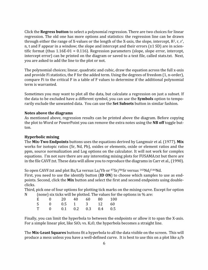
Click the Regress button to select a polynomial regression. There are two choices for linear regression. The old one has more options and statistics: the regression line can be drawn through either the range of X-values or the length of the X-axis, the slope, intercept, R2, r, r', n, t and F appear in a window; the slope and intercept and their errors (±1 SD) are in scien-tific format (thus 1.16E-01 = 0.116). Regression parameters (slope, slope error, intercept, intercept error) can be printed on the diagram or saved to a text file, called stats.txt. Next, you are asked to add the line to the plot or not. The polynomial choices; linear, quadratic and cubic, draw the equation across the full x-axis and provide Fi statistics, the F for the added term. Using the degrees of freedom (1, n-order), compare Fi to the critical F in a table of F values to determine if the additional polynomial term is warranted. Sometimes you may want to plot all the data, but calculate a regression on just a subset. If the data to be excluded have a different symbol, you can use the Symbols option to tempo-rarily exclude the unwanted data. You can use the Set Subsets button in similar fashion. Notes above the diagrams As mentioned above, regression results can be printed above the diagram. Before copying the plot to Word or PowerPoint you can remove the extra notes using the NB off toggle but-ton. Hyperbolic mixing The Mix-Two Endpoints buttons uses the equations derived by Langmuir et al. (1977). Mix works for isotopic ratios (Sr, Nd, Pb), oxides or elements, oxide or element ratios and the ppm, source normalization and Log options on the calculator. It will not work for complex equations. I'm not sure there are any interesting mixing plots for FUSAMA.txt but there are in the file CAVF.txt. These data will allow you to reproduce the diagrams in Carr et al., (1990). So open CAVF.txt and plot Ba/La versus La/Yb or 87Sr/86Sr versus 143Nd/144Nd. First, you need to use the identify button (ID ON) to choose which samples to use as end-points. Second, click the Mix button and select the first and second endpoints using double-clicks. Third, pick one of four options for plotting tick marks on the mixing curve. Except for option N (none) six ticks will be plotted. The values for the options in % are: E 0 20 40 60 80 100 S 0 0.5 1 3 12 60 T 0 0.1 0.2 0.3 0.4 0.5 Finally, you can limit the hyperbola to between the endpoints or allow it to span the X-axis. For a simple linear plot, like SiO2 vs. K2O, the hyperbola becomes a straight line. The Mix-Least Squares buttons fit a hyperbola to all the data visible on the screen. This will produce a mess unless you have a well-defined curve. It is best to use this on a plot like a/b

7

vs. c/d. Because it is quite a fussy equation to fit, a success is a strong positive indicator of mixing, providing, of course, that field data, thin section observations and basic geochemical patterns indicate mixing. A failure here suggests that a mixing case may have imprecise data or that AFC is operating, so the case is not simple. Model (in X-Y plots) Model allows you to calculate paths for fractional or equilibrium crystallization or the AFC (assimilation-fractional crystallization) process. To examine the AFC capabilities properly, you should get DePaolo (1981) and read the file DEPAOLO.TXT. This file will allow you to reproduce Figure 3 in DePaolo's article and, in the process, learn how this modeling works. For a simple test of Model, reload the FUSAMA.TXT file and plot SiO2 vs. K2O. Consider the red symbols for Santa Ana and use ID ON to locate a "parent" on the lower left side of the data array. Now click Model. Select FC for fractional crystallization. Then select the "parent" (Co) and the model parameters. Bulk distribution coefficients of 0.7 for SiO2

and 0.01 for K2O

are good starting points. You can make several models and make a real mess of the graph if you keep all your models. To clean it up, click Aspect, then Quit. A pad of paper is useful to remember what models are worth including in a final plot. Overall, this option is a useful first pass, qualitative way to develop a FC, EC or AFC model. To do this properly you need to consider all pertinent elements at once and include realistic modal and partition coefficient data. This is done in the considerably more powerful model option available with spider diagrams. Error Bars If a data column is followed by a column headed by “error”, Igpet recognizes the second col-umn as the ± error and plots an error bar. To see how error bars work, read the file Boqueron.txt and plot SiO2 versus TiO2. Error propagation will eventually be added but for now error bars work only for single columns. You can calculate propagated errors in Excel. For example, calculate a Ba/La column and place the propagated error in the next column with the header “error.”

Make a Triangular Plot Triangular plots are created from the Plot Menu with the same calculator used for XY plots. To make a triangular plot, click Plot TRI. You will be asked to define the three end members, X, Y, Z, (e.g. Na2O+K2O, FeO+.8998*FE2O3 MgO). (Note: 0.8998 can be inserted in a buffer by pressing C for "constant"). A new button, Quad, allows you to cut off one or more corners of the triangle. Cut the top by specifying 0, .5 when asked for the Min, Max of the Top Apex. This will give a quadrilateral. Cutting the extent of the triangle may allow it to be drawn at a larger size and Igpet will do so automatically.

Make a Spider plot

8

Spider diagrams are a great way to see large variations in incompatible elements at a glance. Because of the log scale you miss the detail seen in XY plots, especially plots of incompatible element ratios. Nevertheless, it is a powerful tool. Unfortunately, there are too many spider-diagrams. The best spider diagrams will eventually win out (I hope). The best, according to reviewers of my work, is primitive mantle normalized. The one by Sun and McDonough (1989) is a good one and there is a revised version, McDonough and Sun (1995). I now use these two almost exclusively, except, of course, for REEs. The general idea of a spider plot is best expressed in the “classic”, the REE plot. The most incompatible element is on the left, the least incompatible element is on the right. The spacing between elements would ideally be related to degree of incompatibility but most diagrams use an ordinal scale to make life easy for draftsmen and computer programmers. For REEs this leads to blank spaces for ele-ments not determined by particular instruments. In Igpet the missing elements show up on the x-axis but no symbol appears (e.g. Pm and Tb). Use Stagger X to get a double or single line for the elements on the x-axis. Repick, NewSpi and Y-Scale are special buttons for the spider diagrams. To see them, first select File-Open File CAVF.txt. Now, select Spider from the Plot menu. From the list of choices that appears try REEs first, by double-clicking on the top entry. Next select a few samples to plot from the list that appears by double-clicking GUM4 and GUT102, from Moyuta and Tecuamburro volcanoes in Guatemala. Use Repick to select different samples, NewSpi to pick a different spider diagram, or Y-Scale to fine-tune the Y-axis. Nrm/Samp allows you to switch to one of your samples as the normalizing standard. That sample plots horizontally at 1. Mixing in Spider plots Explore the Mix option by clicking the button. You can select up to 5 samples that can be mixed using integer weights, decimal fractions or %s. Thus, 3,1 and .75, .25 and 75, 25 produce the same result when mixing two samples. You can average 5 samples by selecting them and giving each a weight of 1. More interesting would be modeling a specific mantle by mixing components, for example, by adding 95 DMM and 5 HIMU. Sr, Nd, Pb, and Hf isotope ratios are also mixed. Logic for eNd, eSr and Os is present but not well tested yet. Modeling in Spider plots Elaborate partial melting, crystallization and assimilation-fractional crystallization (AFC) models can be calculated while a spider diagram is plotted. The Spider model option allows one to sim-ultaneously model fifteen or more elements plus isotope ratios of Sr, Nd, Pb, Hf and epsilon values of Nd and Sr. The elements that are modeled are the ones found in the PC file selected in the SPIMOD window and also present in the data file. The models remain in Igpet’s memory for subsequent use in X-Y plots of elements and isotope ratios and, if desired, can also be saved to a new file. Spider models require partition coefficient files (*.PC.txt files in the folder called PC), a starting composition, and knowledge of melting models. The book by Francis Albarede, Introduc-tion to Geochemical Modeling, should be read carefully before using any of the melting or crys-tallization models. To see examples of how this powerful set of options can be used, see Feigenson et al. (1996) or look for Patino et al. (2000). The CoDoPi option in spider modeling uses a trace

9

element inversion method developed by Feigenson and Hoffman and used in Feigenson et al. (1996). The AFC models of DePaolo (1980) use a parameter r, the ratio of assimilation rate/crystallization rate. For the three cases r<1, r=1 and r>1, different ranges of F are suggested by Igpet. Study the DePaolo paper first, rather than blindly using the software. In the Spider AFC models a parameter called ep_Nd is recognized by Igpet as epsilon Nd. Simi-larly, use ep_Sr for epsilon Sr values. For zero age rocks the Add Extra Parameters function in the File Menu will add eNdo. Igpet recognizes ep_Nd, eNdo, and ep_Sr as isotope ratios and uses DePaolo’s equations 13b and 15b to calculate AFC models. In the data file, Depaolo.txt, are four samples. The first two allow you to recreate DePaolo’s figure 4. The last two allow you to recreate figure 6. One first makes the models in the Spider plot, then makes X-Y plots to reproduce the figures. To use the Model option for melting and assimilation/crystallization processes, start by selecting a model, e.g. Aggregated Fractional Melt, then select whether melting is modal or non-modal (Pi’s<> Di’s). Then pick a partition coefficient file (a pc.txt file), a mantle mode, a melt mode (if non-modal melting), and a set of % melts. For non-modal melting the maximum % melting possi-ble for the chosen mantle and melt mineral assemblages is shown. Keeping that upper limit in mind, adjust the set of % melts. You can run a melt model forward (the default) or backward (inverse) by toggling radio buttons. When all is set, click the Make Calculations button, the bulk D’s will appear, then the P’s in non-modal melting, then the models will be plotted on the spider diagram as black crosses. Unlike the simple models made in the XY plots, these calculated results are now in memory, so you can go on to make XY plots, especially ratio versus ratio diagrams, to look in detail at your models. To save any models permanently, you must go to File-File Operations menu and Save the file. It is always best to save the file using a new name.

Output Options For the professional version of Igpet, the PDF save button creates a pdf file. Igpet suggests a file name that merges the data file name and the diagram axes in a File Save dialog so you can place the file where you want. I suggest creating an IgpetPDF folder on the Desktop be-cause diagrams pile up fast. The PDF output is high quality graphics suitable for publi-cation. The diagrams are superior to any others made on a Mac by earlier Igpet ver-sions. There is an option in Preferences that causes Preview to launch and display the PDF file that was just saved. In Preview, use Edit/Copy to copy your diagram to the Clipboard or Print it. By default this option is off. Diagrams saved to the Clipboard are not always cor-rectly rendered in Adobe Illustrator, however Microsoft Office renders the same diagrams correctly. It is better to save a PDF file and then read it using Adobe Illustrator or Inkscape.

10

Pasting Igpet diagrams directly into Microsoft Office is simple and effective. For Word it is best to right-click or control-click the diagram and select Format Picture. Next, select Lay-out-Tight. You can then place the picture wherever you want. You will be frustrated if you try to ungroup and Igpet diagram in Office. As far as I know, it is no longer possible. To fine-tune a diagram, get an excellent illustration program such as Adobe Illustrator (Ai) or an open source program like Inkscape, which is simpler than Ai and appears to be free. For the teaching version of Igpet, the JPG save button creates a jpg file. Igpet suggests a file name that merges the data file name and the diagram axes in a File Save dialog so you can place the file where you want. I suggest creating an IgpetJPG folder on the Desktop because diagrams can pile up fast. There is an option in Preferences that causes Preview to launch and display the JPG file that was just saved. While in Preview, use Edit/Copy to place your diagram on the Clipboard or use Print to get a hard copy. By default this option is off. Before printing or saving a diagram, explore the buttons of the lower left side of the main window. For printing, the colored backgrounds can waste a lot of ink on drafts, so there is an option for switching back and forth between colored (Color) and white (White) background rectangles. If you don’t like colors at all, you can set the defaults to white (255,255,255) in your favorite sym file. Change boxcolor and pagecolor, located near the top of the file. Use the TextEdit accessory. See section below on symbol files. Page View and Nrml View This toggles the view of either a whole page (portrait or landscape) or the normal view of a single graph, which is the Portrait-Upper page position. Multiple diagrams per page To make a set of eight Harker (SiO2 versus oxide or element) or Fenner plots (MgO versus oxide or element) all on the same page, first activate Page View. Next click menu Plot-Dia-grams and select Harker or Fenner. Plot the first diagram and it will show up on the page view in its proper place. Next click the PDF save button and pick a file name. Next click the Add latest diagram to plot button. Next select the Next diag button, then click the PDF save button and then the Add latest diagram to plot button, etc. When you have plotted all eight figures and added them to the plot, click the PDF save button one last time and se-lect Close/Finish page.

Preferences The Preferences menu brings up a window that allows you to customize Igpet. Four buttons allow you to specify: the font size, the path to the directory where you keep your data files, the file used for symbols and the file used to read the normalization factors for the S-norm function in the Calculator. Radio buttons allow you to select five other options. The first is a file filter that allows you to set limits on the data that will be read from a large data file. This

11

is an old part of Igpet, I suggest using the SubSelect window instead. The second switches the y-axis labels to horizontal or vertical. The third allows you to remove the bounding line from filled symbols, The fourth toggles on or off the background color of the box or triangle where the data plot. The fifth toggles Preview to start (or not) when a diagram is saved. At the upper right of the preferences window is a textbox for scaling the size of the Igpet window. It is advantageous to scale the size of Igpet to be smaller than your screen, this allows Igpet to be a moveable window. Igpet ships with a default width of 1000. I suggest adjusting this so that the Igpet window does not fill the entire screen. The changes you make in preferences will not do much unless you save them. Your choices go into igprefini.txt for use the next time you start Igpet. The radio buttons and any changes to the Misc area take immediate effect but other changes do not. Examine “What_is_igprefini.txt” in the Controls folder if you wish to change the default settings with a text editor.

12

Data Handling in the File Menu Options for Additional Parameters Igpet can calculate and store in RAM a large number of parameters derived from the major and trace element values. The derived parameters can be saved to a file, but this is not usually worthwhile, because it is slower to read such data, than it is to calculate it. If you want to transfer some of these parameters to a spreadsheet, then it may be worthwhile. Before add-ing derived parameters make sure the data matrix has enough room. Reset Matrix Size (File Menu) If you plan to add optional data fields, you should check the current size of the data matrix before you read your data file. Click this menu item to see default matrix size. The first number (rows) tells you the maximum number of analyses. The second number (columns) tells you how many fields are allowed. You start with the number of fields in your data file. Then add the following: CIPW 26 Pearce 17 or more Extra 7 or more Normalize 1 Putting all this stuff into the data matrix means adding about 50 fields. It makes the calculator difficult to use and is usually not necessary. The best plan is spend a session working with the CIPW Norm, then re-read your data file and work with the other parameters. The single data field added by the Normalize routine will be unloaded if nothing else has subsequently been loaded. The other parameters can't be unloaded, to get rid of them, you have to re-read your file. Norm to 100% (File Menu: normalize to 100%, water free, Fe as FeO) If there is a limited range of silica values (e.g. 49-55) in a suite, scalar effects will appear large. The largest analytical error is usually silica, just because it is more than half of most rocks. Other scalar errors occur if the rock is altered (added water, oxidation of FeO, etc.). Further-more, most analyses are subject to minor systematic or gravimetric errors leading to values that are slightly high or low. If errors like these occur then silica will be visibly affected, whereas K2O or other oxides will appear unchanged. This is the general rationale for using this subroutine. These effects are part of the closure problem (Chayes, 1964). The Norm to 100% routine finds 13 oxides: SiO2, TiO2, Al2O3, Fe2O3, FeO, MnO, MgO, CaO, Na2O, K2O, P2O5, Cr2O3, NiO (the last two are typically converted from ppm values) and multiplies them, just before plotting, by:

100/(sum of oxides), in which Fe2O3=0 and FeO=FeO+.8998* Fe2O3 The original data are not changed so you can turn Normalization on and off without getting round off errors. A new parameter, FeOt, is added. It is total Fe as FeO, normalized to 100%. This new parameter will be removed when you turn Normalization off, unless you have sub-sequently added other parameters. Note that FeO* is NOT recognized as one of the 13 oxides and will be ignored by Igpet, causing error. Use only FeO or Fe2O3 as column headers for the oxides of Fe.

13

If you want to normalize trace elements by the same factor as the major elements answer "Yes" to get a list of data fields. The major elements and the trace elements listed in Igpet-data.txt are preceded with * indicating that they will be normalized. To do the same for any other trace elements, double-click the element and an * will be added, telling Igpet to nor-malize this element. When done, move to Quit at the end or beginning and double-click, or click OK. In the Special Diagrams, an XY plot can be normalized to 100% volatile free by adding NMX and/or NMY after the XY diagram discriptor, so the first line of the diagram description be-gins with XYNMXNMY for the LeBas TAS rock-type diagram (setting SiO2 and total alkalies to their normalized values. The normalization is part of the definition of the diagram. Resetting the Ferric/Ferrous ratio Because many data sets present all the Fe as either Fe2O3 or FeO, there is a need to apportion the Fe in a reasonable way. For Pearce element ratios and CMAS projections Igpet has a sub-routine that allows one to us the logic of Kress and Carmichael (1991) to reset the Fe oxides. If you chose to reset the Fe oxides, temperature is determined from lava composition follow-ing Beattie (1993) and fO2 is set following a choice of an oxygen buffer. You can also use the utility program, PTfO2.app, to calculate Fe2O3 and FeO and use the generated values to re-place the Fe oxide values in your data file. I suggest keeping the original data columns under new headers like xFe2O3 and xFeO. Irvine and Baragar (1971) based rock identification on the CIPW Norm. They recalculated FeO and Fe2O3 using Fe2O3=1.5+TiO2. If the analysis value is less than this, no change is made. In the Minerals subroutine, the charge balance logic of Lindsley and Anderson (1983) is fol-lowed to partition the Fe oxides before plotting pyroxenes on the geothermometer. Extra Param. (File Menu) Commonly used calculations can be stored here and automatically made, rather than using Igpet's calculator. The data file "EXTRA.txt" is described in Appendix A. It includes a few standard parameters. The parameter FeO* is FeO+0.8998* Fe2O3 and it has not been nor-malized. Mg# is 100*MgO/(MgO+FeO+0.8998* Fe2O3), where the oxides are first divided by their molecular weights. Ba/La and La/Yb are just what they say. Ce*, Eu*, Nb* are nor-malized values obtained by log interpolation from adjacent REEs. The epsilon Nd value at zero age is eNdo. The value of CHUR is set to 0.512638 and the o subscript indicates that this is a zero age calculation. There are two built in parameters. Density is calculated on a normalized basis with 88% of total Fe as FeO, using the method of Bottinga and Weill (1970). Viscosity is crudely estimated after Giordano et al. (2008), using 1000° C and 2 wt% H2O. Pearce Param. (File Menu)

14

The problem of closure in rock analyses (they add to 100% more or less) makes interpreta-tion of traditional Harker (SiO2) and Fenner (MgO) diagrams inconclusive (see Chayes, 1964). These diagrams allow no simple determination of which minerals or combinations of minerals are being removed (or added) to a magma. The basic problem is that whatever di-rection SiO2 is going, most other oxides must perforce go in the other. What is worse is that although a large percentage of what is removed is SiO2, it usually will go up anyway. A partial solution to the closure problem is to divide the X and Y variables by a common, highly incompatible or conserved element, like K in arc lavas or Ti in tholeiitic basalts. Explaining spe-cific combinations of oxides that will test for the removal of one or more minerals is outside the scope of this guide. Please refer to Pearce (1968), Russell and Nicholls (1988), Stanley and Russell (1989), Russell et al. (1990), Defant and Nielsen (1990).

To test the utility of Pearce Element Ratio diagrams (PER diagrams), read the file, "BOQUERON.txt". Fairbrothers et al. (1978) showed that an older suite at Boqueron had a calcalkaline fractionation path caused by removal of nearly equal proportions of plag and cpx {pl/(cpx+pl)=0.55}; whereas the recent lavas had a tholeiitic path caused by removal of much more plag than cpx {pl/(pl+cpx)=.72}. Olivine, opx and magnetite play a minor role. This result was obtained tediously by making a great many least squares mixing calculations. Now test this with a PER diagram. Let X be (2Ca+Na)/K and let Y be Al/K (Russell and Nicholls, 1988). The slope of the regression should be pl/(pl+cpx) and ol will have no effect. Use the Symbols routine to select one suite and then the other. Make a regression for each. The slope is the pl/(pl+cpx) ratio. The PER diagram method reaches the Fairbrothers et al. conclusion in a flash, the slope for the older lavas is 0.551. For the younger suite the slope is

15

0.703. Although statisticians caution against PER diagrams (see Rollinson, 1993 for sum-mary), sometimes this method produces results compatible with other approaches. CIPW Norms (File Menu) The CIPW Norm is familiar to most geologists. Adding a Norm is essential for the Irvine and Baragar (1971) classification scheme, which is covered in one of the special diagram options. Igpet's CIPW is not complete, but it is serviceable for most uses. The normalization subrou-tine described above does not affect the data that are input to the CIPW subroutine, so, you are asked again if you want to normalize the data to 100% before calculating the Norm.

16

Rock and Mineral Data Files

Igpet’s file reading logic uses tab delimited text files (.txt) or comma delimited text files (.csv). Both are ASCII or flat text files. The file begins with a row of names, one for each column or data field. Columns are separated using tabs. Oxides and other data can be in any order. Tab delimited data file structure The first row is the list of column/field names; each subsequent row is an analysis. dum Jcode Kcode Lcode sample SiO[2] TiO[2] Al[2]O[3] etc. 81 1 4 4 PLA7 50.89 .879 20.21 etc. 81 1 4 4 PLA8 etc. Comma delimited data file structure Replace all the tabs with commas and the .csv files are almost like the .txt files. The difference is that some column headers (variable names) or alphabetic data can have commas in them. Excel knows to bracket such items in quotes, e.g. “Basalt, tholeiitic.” This makes dealing with .csv files more difficult, because software has to recognize the quotes and take steps to han-dle what follows. Regardless of file type, each row is read as a single string and then parsed. Format features The [2] and [3] in the parameter names signify that these are subscripted variables in plots. Similarly, {87} or {86} define superscripts. The first line has 7 reserved words, two of which, Sample (actually the string “samp”) and Kcode, should be included in any file. Sample the sample name, a string variable Mineral* mineral abbreviation, ol, opx, cpx, pl, hb, mt, il, rut, ga, phl, etc Jcode an integer that can be used to control the symbols in plots. Kcode integer variable that is the default control for symbols. Lcode an integer that can also be used to control the symbols. dum placeholder that allows Igpet to ignore any columns not needed. error for drawing error bars, the error in the previous column e.g. SiO[2] error 51.3 .513 for a 1% error in SiO2

* for Mineral files only, not for rocks

17

Using Igpet's File Operations From the File Menu click File Operations. This menu gives you several choices. View data A grid is presented with all the data up to 64 column limit. Save file Warning! Use a new name! The file save dialog box opens and you select a new name and extension, if needed. Add a file (Merge Files) THIS IS OFTEN VERY VERY USEFUL This option allows you to merge two files that have different (or the same) formats. There is a catch. If the second file has data fields (columns) that the first file lacks, these data fields will not be part of the new joint file unless you first add dummy to the first file using the same column headers as are in the second file. This option is useful for merging files with data in different order. Data files to and from spreadsheets via .txt files Excel and other spreadsheets can write tab or comma delimited txt files. Use Excel to maintain your data in the default format (*.xls or *.xlsx). When you are ready to make plots, save the data file as a tab or comma delimited text file (a *.txt or csv file). Use your spread-sheet to update data files; it is much more efficient than a text editor. Comma delimited files (.csv) appear to be the native format for data extracted from GEOROC. Therefore, Igpet now reads these files. However, GEOROC often has empty columns that greatly expand the num-ber of variables in Igpet. These show up as empty buttons on the variable menu. I suggest saving the raw GEOROC extract to a tab delimited file and then removing all the empty col-umns and blank rows, if present. You should also add a Kcode column to assign a variety of symbols to each subset of the data.

18

Pre-designed Diagrams Igneous petrology is full of specialized plots designed for a variety of purposes. Usually the parameters are linear combinations of major oxides in either wt% or molar terms. There are also many trace element ratios. Several derived parameters are commonly used for the X or Y-axis (e.g. Mg#, Ce*, ∑Nd). Earlier versions of Igpet allowed one to formulate these derived parameters but the logic was awkward. The Text box calculator, described above, was created to give Igpet the capacity to parse equations and correctly carry out the func-tions, operations and combinations specified. The new logic is therefore simpler. All the control files that call the equation parser are text files (.txt) that can be modified or added to using a text editor. Mineral Diagrams (in MIN Folder) A few simple mineral plots are created by the control file Minplot.txt in the MIN folder. The first line has 4 entries separated by tabs. MTRI tells Igpet this is a mineral plot and the shape is triangular. Next is the plot name. Third is a string of mineral abbreviations, connected by “+”. Finally, there is a placeholder for the 4th place. The mineral abbreviations identify the minerals that will be plotted. Igpet compares the strings separated by the “+” signs to the Mineral column in the data file. The next three lines define the left, top and right apices of the triangle. Each line consists of Label-tab-Equation. The subsequent line defines the part of the triangle that is plotted. The six entries are leftmin, leftmax, topmin, topmax, rightmin, right-max. A topmax of 0.5 creates the familiar quadrilateral shape. The final two lines are empty, just a zero in each. This tells Igpet there are no interior lines and no labels. MTRI Simple Pyroxene Quadrilateral CPX+OPX dummy

En MgO Wo50 CaO Fs FeO+MnO

0 1 0 .5 0 1 0 0 There are also mineral strings in the partition coefficient (PC) files. So, it is a good idea to coordinate your mineral names in the PC file with the mineral strings in the Mineral column of your data files. The default strings are: ol, opx, cpx, pl, hb, sp, mt, il, rut, ga, phl. You can change these to suit your preferences, just do so systematically in the mineral data files and the mineral diagram files, so that all appropriate minerals get identified and plotted and, also, the PC files, so that the Mixing app will be able to match partition coefficients and minerals. One complex diagram, the Lindsley and Anderson (1983) two pyroxene geothermometer, is included. Fe++/Fe+++ is determined by charge balance in a special subroutine derived from the original publication.

19

CMAS Projections (in CMAS Folder) There are many ways to transform the major elements into the four end-members, C, M, A and S. Elthon (1983) provides a lucid review. The textbook "The Interpretation of Igneous Rocks" by Cox, Bell and Pankhurst (1979-Allen and Unwin, London) has good graphical de-pictions of projections. O'Hara (1976) describes the advantages of "pseudoquaternary isostructural molecular equivalent weight projections". Grove and Baker (1984) suggest that projections should be on an oxide basis, rather than a molar or weight basis. There is no agreement on how best to employ the many projections that exist. Different ones may be suitable for different circumstances. To pursue this, I suggest starting with O'Hara (1976). The Phase boundaries in the plagioclase projections from the Grove groups’s publications include the results of Sack et al. (1987). This results in a straighter cpx-ol boundary, near the cpx-ol sideline. The Grove projections generally assume all Fe is FeO. To allow for this the Igpet versions of the logic add 0.899 times Fe2O3 to FeO. This is useful for rock analyses by XRF where all Fe is treated as Fe2O3. Grove projections also use quantities like AlO1.5. For ease of programming these expressions are kept in mole units and multiplied by 2, so 0.5* AlO1.5 = Al2O3. Special diagrams (in Diagrams Folder) Fenner.txt and Harker.txt are multiple MgO and SiO

2 plots respectively. On a printer the eight

subdiagrams in each file will be packed into the same page in two rows of four. This is a handy way to make a quick survey of a data set. When you are satisfied with the first diagram, click Print. After the plot is sent to the printer buffer, answer NO when asked if this is the last plot on the page. End the plot only after the eighth diagram is done. Discrimination and classification diagrams (in Diagrams folder) DiscrimBasalt.txt, Granite.txt, Komatii.txt, Mantle.txt, Rocktype.txt, Irvbar.txt are files con-taining groups of diagrams that attempt to define (or discriminate) the tectonic environment of rock suites or provide useful nomenclature. IrvineBaragar.txt is the Irvine and Baragar (1971) rock classification scheme. The diagrams and plotting parameters for the Discrim-Basalt file are mostly from Rollinson (1993). For proper use, these discrimination diagrams should be used only in conjunction with the original references or Rollinson (1993)! The in-dex numbers refer to figures in Rollinson’s Chapter 5. Pay attention to the limits set for all the diagrams. First of all DiscrimBasalts is for basalts, so use SubSelect to set maximum and minimum values for SiO2. With rigor I use the TAS limits, 45 to 52. I sometimes relax that to include picro-basalts and basaltic andesites with TAS limits expanded to 41 to 57. The IUGS commission on rock nomenclature sets the rules on how igneous rocks should be named (Le Maitre et al., 2002 and 2010). The IUGS specifies two diagrams based on modal analysis, QPAF plutonic and QPAF volcanic, for the majority of igneous rocks. A few special diagrams are defined for unusual igneous rocks. The primary diagrams are based on the percentages of minerals in the rock as determined by thin section analysis, either by point counting or by image analysis. This approach is more suitable for intrusive rocks, which commonly are completely crystalline. For volcanic rocks, the alternate method is to obtain

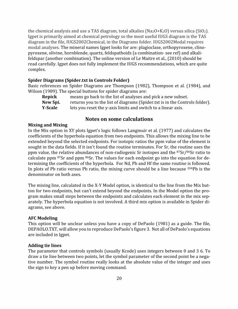
20

the chemical analysis and use a TAS diagram, total alkalies (Na2O+K2O) versus silica (SiO2). Igpet is primarily aimed at chemical petrology so the most useful IUGS diagram is the TAS diagram in the file, IUGS2002Chemical, in the Diagrams folder. IUGS2002Modal requires modal analyses. The mineral names Igpet looks for are: plagioclase, orthopyroxene, clino-pyroxene, olivine, hornblende, quartz, feldspathoids (a combination- see ref) and alkali-feldspar (another combination). The online version of Le Maitre et al., (2010) should be read carefully. Igpet does not fully implement the IUGS recommendations, which are quite complex. Spider Diagrams (Spider.txt in Controls Folder) Basic references on Spider Diagrams are Thompson (1982), Thompson et al. (1984), and Wilson (1989). The special buttons for spider diagrams are: Repick means go back to the list of analyses and pick a new subset. New Spi. returns you to the list of diagrams (Spider.txt is in the Controls folder). Y-Scale lets you reset the y-axis limits and switch to a linear axis.

Notes on some calculations Mixing and Mixing In the Mix option in XY plots Igpet's logic follows Langmuir et al. (1977) and calculates the coefficients of the hyperbola equation from two endpoints. This allows the mixing line to be extended beyond the selected endpoints. For isotopic ratios the ppm value of the element is sought in the data fields. If it isn't found the routine terminates. For Sr, the routine uses the ppm value, the relative abundances of non-radiogenic Sr isotopes and the 87Sr/86Sr ratio to calculate ppm 87Sr and ppm 86Sr. The values for each endpoint go into the equation for de-termining the coefficients of the hyperbola. For Nd, Pb and Hf the same routine is followed. In plots of Pb ratio versus Pb ratio, the mixing curve should be a line because 204Pb is the denominator on both axes. The mixing line, calculated in the X-Y Model option, is identical to the line from the Mix but-ton for two endpoints, but can't extend beyond the endpoints. In the Model option the pro-gram makes small steps between the endpoints and calculates each element in the mix sep-arately. The hyperbola equation is not involved. A third mix option is available in Spider di-agrams, see above. AFC Modeling This option will be unclear unless you have a copy of DePaolo (1981) as a guide. The file, DEPAOLO.TXT, will allow you to reproduce DePaolo's figure 3. Not all of DePaolo's equations are included in Igpet. Adding tie lines The parameter that controls symbols (usually Kcode) uses integers between 0 and 3 6. To draw a tie line between two points, let the symbol parameter of the second point be a nega-tive number. The symbol routine really looks at the absolute value of the integer and uses the sign to key a pen up before moving command.

21

Common Problems

Zeros are not plotted In all the graphs X, Y, or Z values of zero are not plotted, because in most data sets 0 means not determined or below detection limit. Errors in a data file If Igpet fails to completely read a file, the matrix limits may have to be changed or the file may be corrupt. A corrupt file has either too many or too few elements in some analysis. To find out where the problem is, go immediately to the File Operations menu and select View. You should be able to track down the error by locating where the data become out of place. Sometimes the only error is a few invisible extra lines or spaces at the very end of a file. When you have located the error, use TextEdit to fix the problem. Points are shifted right in the TAS diagram This diagram was designed by the authors using data normalized to 100% water free with all Fe as FeO. Most analyses sum to less than 100% without water so normalization often shifts SiO2 to noticeably higher values. This is not a problem. Too Many Fe parameters Some data sets include Fe2O3 and FeO where both are determined separately. This is the correct presentation but it is no longer common. Most modern data sets have only Fe2O3 or only FeO with the other oxide set to zero. This is the best situation for Igpet, which has built in routines for apportioning the Fe between the two oxides. Serious error occurs if the data set includes both oxides and puts all the Fe into both. Some Igpet functions use both Fe ox-ides so putting all the Fe into both Fe-oxide columns doubles the amount of Fe seen by the Igpet functions and causes error. Failure of International awareness Igpet tries to read data files in the format appropriate for each country. In the United States the period is the decimal marker but in many other countries it is the comma. A function called CStr id supposed to take care of this but it sometimes fails. Therefore Igpet has a backup routine that recognizes the period as the decimal marker, so a file in US format can be read by Igpet regardless of the International setting. If you data file fails to read properly, save a new version after changing the format to US settings (period as decimal marker and no other punctuation for numbers.

22

Mixing.app This program makes petrologic mixing calculations using least squares regression of the ma-jor elements, after Bryan et al., (1969). Trace element calculations are made, based on the major element solution. Many researchers use this technique to test the plausibility of mod-els of crystal fractionation or magma mixing. What criteria to use to judge whether a model is permissible is debatable and can vary with the problem being addressed. In general, the residuals (the difference between observed and calculated) should be within analytical er-ror. However, low residuals are no guarantee that the model is successful. The high degree of covariation of major elements really means that there are few degrees of freedom. There-fore, some successful appearing fits may be nonsense. The best you can say of a model with low residuals is that it has not been rejected, but it certainly cannot be proved with this tech-nique. The good news is that a great many models fail and can be rejected, so this a valuable tool within its limits. To start MIXING, click on the MIX icon. MIXING starts with its main menu. First read a partition coefficient file (.PC.txt). If you will be ignoring trace elements select Null.PC.txt. Next, select a weighting function for oxides file (.wt.txt). Click the View PCs button and note that there is 0 weight for Fe2O3. This is a re-minder that Mixing puts all the Fe in to FeO. Now read a mineral file and a rock file. You can read new mineral, rock or PC.txt files at any time. The partition coefficient files hold the partition coefficients needed for trace element calcu-lations. The weights files hold the weighting values for the major oxides. Different partition coefficient files should be created for different types of rock suites. Select the partition coef-ficient file you want (e.g. Gill.PC.txt). Trace elements do not contribute to the solution but can help as a separate check on the solution. Incompatible elements behave well because they are simply concentrated in the residual liquid. In the Raleigh equation F is % liquid, the Cs are concentrations and D is the weighted sum of partition coefficients, the bulk partition co-efficient of the cumulate crystals. The Raleigh equation is Cliq = Co . F (D-1). For incompatible elements (e.g. those with D values near zero) the equation simplifies to Cliq = Co/F. For com-patible elements, those strongly partitioned into phenocrysts (D>1), the changes in concen-tration as F decreases are very large and very susceptible to error in partition coefficients. View PCs, button at the lower left, lists the partition coefficient and weighting data. Check it for correctness. The mineral abbreviations at the top of the matrix are strings that will be looked for in the mineral file you read. One of these strings needs to match the mineral ab-breviations in the Mineral column of the data file for MIXING to tie a set of partition coeffi-cients to the mineral. In Gill.PC.txt plagioclase is "pl". Thus, a plagioclase in a mineral file has to have "pl" in the column labeled “Mineral.” The weight for each oxide data allows you to reduce the effect of the overwhelming predom-inance of SiO

2 and Al

2O

3 in most analyses. Before least squares calculation, each oxide will

23

be multiplied by its "weight". The analyses are then printed in un-weighted form, but the residuals and sum of squares of residuals are weighted values. If a weight file has weights of 0.4 for silica and 0.5 for alumina, there will be a discrepancy for these oxides between the difference between the Observed and Calculated magmas and the calculated (weighted) re-sidual. You can change the weights to 1.0 to eliminate this, but then you will be giving silica and alumina more control over the result. You can also give an oxide a weight of 0.0 and it will not contribute to the least squares solution. Now load data files and begin making models. Start with Gill.PC, CerroNegroGeochem and cerronegro.min and reproduce the published examples in Walker and Carr (1986). The usual model is Fractional Crystallization (Fract. Xtl.) First, pick minerals. It's unwise to pick two or more of the same minerals, e.g. two olivines. Second, pick a daughter Third, pick a parent. (You can reverse these if you prefer.) The general equation is:

parent = (c1, c2, c3,..., cd) * (min1, min2, min3,...., daughter) Mixing solves for the coefficients (c's). The result is seen as soon as you finish your selection. Output goes first to the screen, but you can send a copy to a text file or a corrected rock file. The last option allows you to build a file of fractionation corrected data, which is useful for trace element modeling.

24

PTfO2.app This interactive program demonstrates how Fe2O3 and FeO vary depending on composition (Xi) and assumptions made about pressure and the appropriate oxygen buffering. Temper-ature is calculated from Xi and P following the equations of Beattie (1993). Oxygen buffers (NNO, QFM and IW) and pressure (P in Gpa) can be selected and the T, P, and fO2 are then used to partition Fe between Fe2O3 and FeO following Kress and Carmichael (1991). Be-cause the T logic is based on partitioning of Mg/Fe between olivine and melt, this logic is primarily for basalts and more mafic magmas in the temperature range 1000°C to 2000°C. Results for silicic rocks are likely to be highly unreliable. The fO2 buffers used are: NNO (O’Neill and Pownceby, 1993) fo2 = (-478967 + 248.514 * T - 9.7961 * T * Log(T)) / (8.31441 * T * 2.302585) QFM (O’Neill, 1987) fo2 = (-587474 + 1584.427 * T - 203.3164 * T * Log(T) + 0.09271 * T ^ 2) / (8.31441 * T * 2.302585) IW (O’Neill and Pownceby, 1993) fo2 = (-550915 + 269.106 * T - 16.9484 * T * Log(T)) / (8.31441 * T * 2.302585)

1000 1500 2000 -

-

-

0

Temp C

QF

fO2 NNO

25

Appendix A: Control Files Igprefini.txt and Igpetdata.txt These files control the IGPET system. You should modify Igprefini.txt using the Preferences menu and the resize matrix and font menus. Igpetdata.txt is basic data in tab delimited rows. Part of the file is shown below. 60.084 79.899 101.96 159.69 71.846 70.937 40.311 Mol wts of 14 oxides 1 1 2 2 1 1 1 number of cations SiO2 TiO2 Al2O3 Fe2O3 FeO MnO MgO oxide name Si Ti Al Fe Fe Mn Mg ppm name 4674 5995 5292 6994 7773 7745 6028 convert to ppm 26.75 22.45 37.8 44.4 13.94 14 12.32 partial molar volumes %AN Q or ab an lc ne CIPW norm names -2.15 0 -8.35 0 -4.5 0 -5.44 Sack et al 1980 to reset Fe++/Fe+++ (no longer used) {87}Sr/{86}Sr labels Igpet will recognize and may adjust {143}Nd/{144}Nd e.g. convert 87sr/86sr to {87}Sr/{86}Sr {206}Pb/{204}Pb {207}Pb/{204}Pb {208}Pb/{204}Pb {10}Be Be Li etc DEFAULT.NRM.txt in the normalization used in the S-Norm button on the calculator. Set the file you want in the preferences window. Note that the first line is a comment. 'Sun and McDonough 1989 primitive mantle Cs .0079 Tl .005 Rb .635 Ba 6.989 W .02 Th .085 U .021 Nb .713 Ta .041 K 250

26

Page.txt controls where Igpet draws its plots. There are 16 options. 8000 10250 ‘page width-height in Portrait mode in 1000's of an inch 16 Portrait 2000 4000 7000 7500 XYL Portrt-Upper 2000 6500 7000 10000 XYL Portrt-Lower 2000 2000 7000 5500 XYL Portrt-UUL 1400 7200 3900 8950 -YL Portrt-MUL 1400 5300 3900 7050 -YL Portrt-LML 1400 3400 3900 5150 -YL Portrt-LLL 1400 1500 3900 3250 XYL Portrt-UUR 4100 7200 6700 8950 -YR Portrt-MUR 4100 5300 6700 7050 -YR Portrt-LMR 4100 3400 6700 5150 -YR Portrt-LLR 4100 1500 6700 3250 XYR Lndscp-Page 2500 2500 9500 7500 XYL Lndscp-LL 1500 1700 5000 4200 XYL Lndscp-LR 5500 1700 9000 4200 XYR Lndscp-UL 1500 5100 5000 7600 XYL Lndscp-UR 5500 5100 9000 7600 XYR

27

Symbol files Default.sym.txt is the file Igpet loads initially to make symbols. Symbol files are tab delimited with 6 columns, the last of which is a polygon, a circle or a line definition. There are two colors, line and fill, that can easily be customized. Using Excel one can move things around and insert new colors. Shapes or polygons can be designed using graph paper. The polygon units are 1/1000 of an inch. The first number is a global scale factor takes the raw polygons and expands (not a good idea) or contracts them all. There is room for 36 symbols! Lines and symbols are created from six columns of alphanumeric data. The first two, number and description, are not used but are needed as place holders. Line color|width is a color R|G|B|, fol-lowed by a width of 15. Fill color is an RGB group, R|G|B. Shape type is self-explanatory. The 6th column is a definition of a circle, polynomial or line.

number description Line color|width Fill color ShapeType

0.5 scale factor for symbols x x x

14 font size x x x

1 tickpencolor-width 0|0|0|15 x x

2 mixmodpencolor-width 0|0|0|20 x x

3 pagecolor 255|255|255 x x

4 boxcolor 255|255|220 x x

5 textcolor 0|0|0 x x

-1 openCircle for ticks 0|0|0|1 0|0|0 CIRC

0 openCircle 0|0|0|1 0|0|0 CIRC

1 openTriangle 0|170|85|15 255|255|255 POLY

…… filledCircle 225|0|0|1 255|0|0 FCIRC

9 + 0|0|0|15 0|0|0 LINE

10 asterisk 0|0|0|15 0|0|0 LINE Circle, polygon and line examples CIRC 1|50|50 defines a circle with one xy pair which defines a radius of 50 POLY 4|130|-74|0|152|-130|-74|130|-74 defines a polygon with 4 points (a triangle) FPOLY 5|-112|-112|112|-112|112|112|-112|112|-112|-112 filled polygon with 5 points (a box) LINE 6|0|-112|0|112|0|0|112|0|-112|0|0|0 line form made of 6 points (a plus sign)

28

SPIDER.Txt This file controls spider diagrams. First line is: title, normalization factor Second line is: 15 x 1 1000 15 elements, x=no double norm, y axis min, y axis max Third line is element list Fourth line is normalization factor Sun+McDon. 1989-REEs Chondrites 15 x 0.7 500 La Ce Pr Nd Pm Sm Eu Gd Tb Dy Ho Er Tm 0.237 0.612 0.095 0.467 1 0.153 0.058 0.2055 0.0374 0.254 0.0566 0.1655 0.025 Nakamura 1974-REEs Chondrites 15 x 1 1000 La Ce Pr Nd Pm Sm Eu Gd Tb Dy Ho Er Tm .33 .865 .112 .63 1 .203 .077 .276 .047 .343 .07 .22 .03 Sun+McDon. 1989 Primitive Mantle 22 x 1 1000 Cs Rb Ba Th U Nb K La Ce Pb Pr Sr P .0079 .635 6.989 .085 .021 .713 250 .687 1.775 .071 .276 21.1 95 Sun+McDon. 1989 Primitive Mantle double norm 23 Yb=10 1 1000 NOTE double norm to Yb and set all normalized Yb values to 10. PercentFs.txt This file sets the suggested F values (in percent) for common melt and crystallization models. Fs_AFC_r=1 0,10,20,30,40 Fs_AFC_r<1 100,95,90,85,80 Fs_AFC_r>1 100,110,120,130 Fs_Equimelt 1,5,10,15,20,25 Fs_FracMelt .1,.5,1,5 Fs_AggFracMelt 1,5,10,15,20,25 Fs_ContinMelt .1,.5,1,5 Fs_RayFracXtal 100,90,80,70,60 Fs_EquiXtal 100,90,80,70,60 Fs_InSituXtal 90,70,50

29

EXTRA.txt This file has parameters that are automatically calculated and added to the variable list when the menu item, file operations - extra is selected. Each extra parameter has three entries; the label is first, the odd string zerosin or nozeros is second and the equation is third. In some equations the lack of a component makes the resulting expression meaningless. For example, if Nb+Ta is called for and the data set contains Nb but only some Ta values, then the Nb+Ta equation will yield a false result wherever Ta is absent, thus “nozeros” is appropriate. On the other hand, if the parameter is FeO +0.8998*Fe2O3, there are many data sets that lack one or the other of these oxides so one uses “zerosin.” The CIPW norm famously sets some nor-mative minerals to zero so many combinations of CIPW normative minerals (e.g. an+ab+.6*ne) require “zerosin.” The extra routine adds two fixed items, density and viscosity. Density is calculated on a nor-malized basis with 88% of total Fe as FeO, using the method of Bottinga and Weill (1970) on a water-free, 1 atm, 1200° C basis. Viscosity estimates are at with 2% water and 1000° C after Giordano et al. (2008). The eNdo parameter assumes zero age! Do not use this for older rocks! Create your own ep_Nd values using Exel. Save calculated epsilon values as ep_Xy, where Xy is an element with isotope ratios like Sr or Nd. FeO* zerosin FeO+Fe2O3*.8998 Mg# zerosin MgO*2.481/(MgO*.0248+FeO*.013918+Fe2O3*.012523) Ba/La nozeros Ba/La La/Yb nozeros La/Yb U/La nozeros U/La Ba/Th nozeros Ba/Th Zr/Hf nozeros Zr/Hf Zr/Nb nozeros Zr/Nb eNd[o] nozeros "{143}Nd/{144}Nd"*10000/.512638-10000 Nb/Nb+ nozeros (Nb/0.713)/((U/0.021)*(K2O*8301/250))^0.5 Nb/Nb* nozeros (Nb/0.713)/((Th/0.085)*(La/0.687))^0.5 Eu/Eu* nozeros (Eu/0.058)/((Sm/0.153)*(Gd/0.2055))^0.5 Ce/Ce* nozeros (Ce/0.612)/((La/0.237)*(Pr/0.095))^0.5 Nb+ is an interpolation between K and U. K is K2O times 8301. KN is K/250 UN is U/0.021 Nb* is an interpolation between Th and La. Diagrams Folder These files allow for predefined diagrams. The control data differentiate XY vs. TRI diagrams, define the X, Y, and Z parameters, define dimensions, interior lines and labels. Some diagrams

30

are complex. Look at some examples, drawn from various files, to learn how to mimic them. Replace "XY" with "XYSMALL" if you want small fonts for interior labels. The delimiter, sep-arating fields, is a tab. The first line consists of 4 entries: diagram control, the label, the source and a comment. The first entry is very important; the others are not. The next three lines define the left, top and right apices of the triangle. Each line consists of Label-tab-Equation. The subsequent line de-fines the part of the triangle that is plotted. The six entries are leftmin, leftmax, topmin, top-max, rightmin, rightmax. Next comes an 18, which tells Igpet that there are 18 interior line segments. The next 18 lines are left, top, pen control, where 1 is down and zero is up. The next line is an 8 telling Igpet there are 8 labels. The next 8 lines are the left, top values and the label. It is important that the oxide or element names used here are the same ones used in the data files. Igpet will compare names on an all uppercase basis with {, }, [, ] stripped out. TRI Zr-Ti/100-Y*3 Pearce+Cann 1973 5.1 Thol. basalts with CaO+MgO 12-20% Zr Zr Ti/100 TiO2*59.95 Y*3 Y*3 0 1 0 1 0 1 18 .555 .24 0 .59 .28 1 .385 .50 1 .24 .48 1 …………………..several lines cut 8 .5 .2 C .4 .4 D .27 .37 A .35 .3 B -.1 .75 Island-arc A B -.1 .60 Ocean-floor B -.1 .45 Calc-alkali B C -.1 .30 Within-plate D This triangular plot adds ZEROSIN to the diagram control string, allowing forgiveness if FeO or Fe2O3 is not measured. The diagram label is AFM. TRIZEROSIN AFM thol vs calc-alk Irvine+Baragar 71 Alk Na2O+K2O FeO* FeO+Fe2O3*.8999 MgO MgO 0 1 0 1 0 1 …………………..several lines cut

31

The next example is an X-Y plot. It has the same first line as the TRI plot: the diagram control, the label, the source and a comment, in this case referring to a diagram in Rollinson’s book. The next two lines are: the Xaxis label-tab-equation and: Yaxis label-tab-equation. The next two lines control the axes, first x and then y. The initial zero says this is not a log plot. The 0 tab 200 sets the range of the x-axis, the two 100s tell Igpet that the tick step is 100 and the label step is 100. An axis control line is: linear=0 or log=1, beginning of range, end of range, tick-step, label-step XY Zr vs Ti Pearce+Cann 1973 5.2a Thol. basalts with CaO+MgO 12-20% Zr Zr Ti TiO2*5995 0 0 200 100 100 0 0 14000 1000 5000 21 135 7100 0 113 7400 1 89 7400 1 ……..many lines cut then 5 labels with: x tab y tab label 5 15 2000 IAT 55 6000 B 125 4000 Calc-alkali basalt 100 9000 MORB 20 12000 B=MORB+C-A bas+IAT The following example includes division (A/B). This plot must have ZEROSIN in the diagram control field because ne is usually zero. Note that the x-axis is reversed going from 100 to 40. XYZEROSIN %An-Al2O3 thol vs calc-alk Irvine+Baragar 71 AN an*100/(an+ab+.6*ne) Al[2]O[3] Al2O3 0 100 40 10 10 0 10 25 1 5 7 40.000 15.200 1 50.000 16.000 1 60.000 16.800 1 70.000 17.600 1 80.000 18.400 1 90.000 19.200 1 100.000 20.000 1 2 90 15 Tholeiitic 90 22 Calc-Alkaline

32

The following example draws a box shape and uses a log scale for x and y. For a log scale the tick-step and label-step are set to zero. They need to be included even thought they are ig-nored. XY BOX Y+Nb vs Rb Pearce et al. 84 Y+Nb Y+Nb Rb Rb 1 2 2000 0 0 1 1 2000 0 0 7 2 80 0 55 300 1 400 2000 1 55 300 0 50 1 1 51.5 8 0 2000 400 1 4 5 750 syn-COLG 300 600 WPG 6 3 VAG 300 8 ORG MIN folder The format of these files is similar to the triangular diagram files. The 2nd to last entries in the first line define which minerals to plot. There is some flexibility. MTRI Feldspars PL+FS+OR+ab+an Feldspars Ab 2*Na2O Or 2*K2O An CaO 0 1 0 1 0 1 24 0 0.1 0 0.5 0.1 1 0.577708491 0.132783019 1 0.597891038 0.212617925 1 etc MTRI Pyroxene Quadrilateral CPX+opx Pyroxenes En MgO Wo50 CaO Fs FeO+MnO 0 1 0 0.5 0 1 12 0.95 0.05 0 0 0.05 1 0.475 0.05 0 etc

33

CMAS folder The format of these files is slightly different from that for the triangular files for regular dia-grams. The diagram’s control parameter CTRI tells Igpet that this is a CMAS projection with three extra data, the final apex scaling values. These numbers follow the apex labels. They are all 1 in this case (molar) but can be in weight or oxygen units. CTRI Plag. Proj. Walker et al 79 Sack et al 87 mole OL 1 .5*Al2O3-.5*Fe2O3+.5*FeO+.5*MnO+.5*MgO-.5*CaO-.5*Na2O-.5*K2O DI 1 CaO+Na2O+K2O-Al2O3 SIL 1 SiO2-.5*Al2O3+.5*Fe2O3-.5*FeO-.5*MnO-.5*MgO-1.5*CaO-5.5*Na2O-5.5*K2O 0 1 0 1 0 1 27 .4535 .708 0 .4169 .58802 1 .3825 .472 1 .3457 .379 1 …. Many lines cut 1 .55 -.07 Opx This example includes “zerosin” in the diagram control field because many analyses lack Cr2O3 or NiO. This also gives an example of scaling by wt% and the triangle is shaved in all three axes. CTRIzerosin M2S to CS60-A30-MS O'Hara 1968 WT CS-60 116.16 CaO+Na2O*2+K2O*2-P2O5*3.333 A-30 101.96 TiO2+Al2O3+Cr2O3+Fe2O3+Na2O+K2O MS 100.4 SiO2*2+TiO2-FeO-MnO-NiO-MgO-CaO*2-Na2O*8-K2O*8+P2O5*6.666 0 .6 0 .3 .4 1 2 .54 0 0 .275 .245 1 4 .58 -.03 CMS[2] .12 .09 AV .29 .255 Ol-Pl .005 .245 - M[3]AS[3]pyrope

34

PEARCE.txt Pearce diagrams are based on element proportions, E. E= (wt% * # of cations)/molecular wt. These are calculated for all the oxides in the Pearce subroutine. Pearce.txt consists of mean-ingful combinations of these element proportions. Consult Stanley and Russell (1989) for the appropriate use of these parameters. In the file, each line consists of label-tab-equation. K K2O Ti TiO2 P P2O5 Si SiO2 Al Al2O3 0.5(Mg+Fe) 0.5*FeO+0.5*MgO OL+CPX+PL 1.5*CaO+.25*Al2O3+0.5*FeO+0.5*MgO+2.75*Na2O (Ca+.5Na-.5Al) CaO+.5*Na2O-.5*Al2O3 (2Na+Al) 2*Na2O+Al2O3 (2Ca+Na-Al) 2*CaO+Na2O-Al2O3 (Si-.25Al-.5FM-1.5Ca-2.75Na) SiO2-.25*Al2O3-.5*FeO-.5*MgO-1.5*CaO-2.75*Na2O (-Si+.5Al+FM+Ca+2.5Na) .5*Al2O3+FeO+MgO+CaO+2.5*Na2O-1*SiO2 (.5FM+2Ca+3Na) .5*FeO+.5*MgO+2*CaO+3*Na2O (2Ca+3Na) 2*CaO+3*Na2O (.5FM+1.5Ca) .5*FeO+.5*MgO+1.5*CaO (2Ca+Na) 2*CaO+Na2O

35

Partition Coefficient files These files are control files for MIXING and modeling in plots. They have the partition coef-ficient data. Gill1981.PC.txt, shown below, is a tab delimited file. el/min PL CPX OPX OL HB MT GA IL K 0.11 0.02 0.01 0.01 0.33 0.01 0.01 0.01 Rb 0.07 0.02 0.02 0.01 0.05 0.01 0.01 0.01 Sr 1.8 0.08 0.03 0.01 0.23 0.01 0.02 0.01 Ba 0.16 0.02 0.02 0.01 0.09 0.01 0.02 0.01 Zr 0.01 0.25 0.1 0.01 0.4 0.4 0.5 0.4 Ni 0.01 6 8 58 10 10 0.6 10 Cr 0.01 30 13 34 30 32 22 32 V 0.01 1.1 1.1 0.08 32 30 8 30 Weight files These files are control files for MIXING. They have the weighting scheme for the oxides. Default.wt.txt, shown below, is a tab delimited file. SiO2 TiO2 Al2O3 FeO MnO MgO CaO Na2O K2O P2O5 NiO Cr2O3 0.4 1 0.5 1 1 1 1 1 1 1 1

36

Appendix B: Data Files COTLO.TXT contains glasses that were formed in equilibrium with Plag-Cpx-(Ol or Opx). These

glasses trace the 1 atm pseudo-quaternary cotectic that exists at the intersection of the primary phase volumes of these minerals. There is a problem in locating this intersection because additional components, especially K

2O and Na

2O, appear to cause large shifts in the location of this intersec-

tion. Different CMAS projections cause different shifts. The problem is to determine how much of the shift is real and caused by thermodynamic effects and how much is an artifact of projection. The partitioning of Fe between Fe++ and Fe+++ was calculated using the equation from Kress and Carmichael (1991) and the T and fO2 data in the original publications. The different Key numbers in this file stand for different data sources. key symbol ref. description 4 filled box Walker et. al., 1979 OFZ 7, 8 circles Grove et al., 1982 Med._Lake, opx, cpx 11 asterisk Grove and Bryan, 1983 Famous 2 filled triangle Baker and Eggler, 1983 Atka 30 red stars Sack et al., 1987 alkaline etc COTHI.TXT contains glasses that were in equilibrium with a dry peridotite sandwich at various pressures. For a complete discussion read Takahashi and Kushiro (1983), the source of most of the data. One data point, plotted as a "X", is from Baker and Eggler (1983). This point represents about 8 kb and an unspecified small per cent H

2O. It was not in equilibrium with a peridotite sandwich.

Because of the water and the type of experiment, it is not strictly comparable to the rest of the data. Fe was not partitioned in the high pressure results because the use of a graphite layer in the exper-imental charge prevented the formation of detectable Fe2O3. The different Key numbers refer to pressures. Key symbol pressure (kb) 1 Gpa=10 kb 1. open triangle 5 0.5 2. filled triangle 8 0.8 3. open box 10 1.0 4. filled box 10-10.5 1.0-1.05 5. open diamond 20 2.0 6. filled diamond 25 2.5 7. open circle 30 3.0 8. filled circle 35 3.5 11. X 8 (wet) 0.8 (wet) VGGP.TXT

37

MORB glass data set provided by Melson et al. (1977). It is a large file of high quality probe analyses of mid ocean ridge glasses from dredge hauls. An even larger file is available on the Smithsonian web site.

Several other data files refer to studies of Central American volcanoes. FUSAMA.TXT Fuego key=1, see: Chesner and Rose (1984) Santa Ana key=7, see: Carr and Pontier (1981) Masaya key=3, see: Walker et al. (1993) CERRONEG.TXT Cerro Negro volcano in Nicaragua, see: Walker and Carr (1986) CN.MIN see above: this file has mineral analyses from Cerro Negro volcano, Nicaragua IZALCO.TXT see: Carr and Pontier (1981) on Izalco volcano, El Salvador BOQUERON.TXT see: Fairbrothers et al. (1978) on Boqueron volcano, El Salvador CAVF.TXT see: Carr et al. (1990)

38

Appendix C: References Albarede, F., 1995, Introduction to Geochemical Modeling, Cambridge Univ. Press, New York, 543 pp. Arndt, N.T., 1976. Ultramafic rocks of Munro Township and Their Volcanic Setting: Unpub. Ph.D Thesis, Univ. of Toronto, Toronto. Bailey, J.C., 1981. Geochemical criteria for a refined tectonic discrimination of orogenic andesites. Chemical Geology, 32 (1-2), p. 139-154. Baker, D.R. and Eggler, D.H., 1983. Fractionation paths of Atka (Aleutians) high-alumina basalts:

constraints from phase relations. J. Volc. Geotherm. Res. 18:387-404. Baker, D.R. and Eggler, D.H., 1987. Compositions of anhydrous and hydrous melts coexisting with plagioclase, augite, and olivine or low-Ca pyroxene from 1 atm to 8 kbar: Application to the Aleutian volcanic center of Atka. Am. Mineral. 72:12-28. Barker, F. 1979. Trondhjemite; definition, environment and hypotheses of origin. In Barker, F. (ed.), Trondhjemites, dacites, and related rocks, p. 1-12. Bedard, J.H., 2001. Parental magmas of the Nain Plutonic Suite anorthosites and mafic cumulates: a trace element modelling approach. Contrib. Mineral Petrol (2001) 141: 747-771. Bottinga, Y. and Weill, D.F., 1970. Densities of liquid silicate systems calculated from partial molar volumes of oxide components. Am. J. Sci. 269:169-182. Brown, G.C., 1982. Calc-alkaline intrusive rocks: their diversity, evolution, and relation to vol-canic arcs. in Orogenic Andesites, R.S. Thorpe ed. John Wiley, p.437-461. Bryan, W.B. Finger, L.W. and Chayes, F., 1969. Estimating proportions in petrographic mixing equations by least-squares approximation. Science, 163:926-927. Cabanis, B., Lecolle, M., 1989. Le diagramme La/10-Y/15-Nb/8; un outil pour la discrimination des series volcaniques et la mise en evidence des processus de melange et/ou de contamination crustale. Comptes Rendus de l'Academie des Sciences, Serie 2, Mecanique, Physique, Chimie, Sciences de l'Univers, Sciences de la Terre, 309 (20), p. 2023-2029 Carr, M.J., 1984. Symmetrical and segmented variation of physical and geochemical characteris-tics of the Central American volcanic front. J. Volc. Geotherm. Res. 20:231-252.

39

Carr, M.J., Feigenson, M.D. and Bennett, E.A., 1990. Incompatible element and isotopic evidence for tectonic control of source mixing and melt extraction along the Central American arc. Contribs. Mineral. Petrol. 105:369-380. Carr, M.J. and Pontier, N.K., 1981. Evolution of a young parasitic cone toward a mature central vent; Izalco and Santa Ana volcanoes in El Salvador, Central America. J. Volc. Geotherm. Res. 11:277-292. Cawthorn, R.G. and O'Hara, M.J., 1976. Amphibole fractionation in calc-alkaline magma genesis.

Am. J. Sci. 276:309-329. Chayes, F., 1964. Varience-covarience relations in some published Harker diagrams of volcanic suites. J. Petrol. 5:219-237. Chesner, C.A. and Rose W.I. Jr., 1984. Geochemistry and evolution of the Fuego volcanic com-plex, Guatemala. J. Volc. Geotherm. Res. 21:25-44. Cox, K.G., Bell, J.D. and Pankhurst, R.J., 1979. The Interpretation of Igneous Rocks, Allen and Unwin, London. 450p. Cross, W., Iddings, J.P., Pirsson, L.V. and H.S. Washington. 1902. A Quantitative Chemico-min-eralogical Classification and Nomenclature of Igneous Rocks. J. Geol., 10:555-690. Davis, J.C. 1973. Statistics and Data Analysis in Geology. John Wiley & Sons, New York, 550 pp. Defant, M.J. and Nielsen, R.L., 1990. Interpretation of open system petrogenetic processes: Phase equilibria constraints on magma evolution. Geochim. Cosmochim. Acta, 54:87-102. DePaolo, D., 1981. Trace element and isotopic effects of combined wallrock assimilation and frac-tional crystallization. Earth Planet. Sci. Let., 53:189-202. Eiler, J.M., M.J. Carr, M. Reagan, E. Stolper, 2005. Oxygen isotope constraints on the sources of Central American arc lavas, Geochem. Geophys. Geosyst. (G3), 6, Q07007, doi:10.1029/2004GC000804. Elthon, D., 1983. Isomolar and isostructural pseudo-liquidus phase diagrams for oceanic basalts.

Am. Mineral. 68:506-511. Fairbrothers, G.E., Carr, M.J. and Mayfield, D.G., 1978. Temporal magmatic variation at Boque-ron volcano, El Salvador. J. Volc. Geotherm. Res. 67:1-9.

40

Feigenson, M.D., Patino, L.C. and Carr, M.J., 1996. Constraints on partial melting imposed by rare earth element variations in Mauna Kea basalts. J. Geophys.Res. 101:11815-11829. Feigenson, M.D., Bolge, L.L., Carr, M.J. and Herzberg, C.T., 2003. REE Inverse Modeling of HSDP2 Basalts: Evidence for Multiple Sources in the Hawaiian Plume. Geochemistry, Geophys-ics, Geosystems (G3), posted 20 February 2003, 25pp. Floyd, P. A. and Winchester, J. A., 1975. Magma-type and tectonic setting discrimination using immobile elements. Earth Planet. Sci. Lett., 27, p. 211-218. Frost, B.R, C.B. Barnes, W.J. Collins, R. J. Arculus, D.J. Ellis and C.D. Frost. 2001. A geochem-ical classification for granitic rocks. J. Petrol. 42:11:2033-2048. Giordano D, Russell, JK and Dingwell, DB, 2008. Viscosity of magmatic liquids: A Model. EPSL [doi:10.1016/j.epsl.2008.03]. Gill, J.B., 1981. Orogenic Andesites and Plate Tectonics. Springer, Berlin 389 p. Gromet, L.P., Dymek, R.F., Haskin, L.A., and Korotev, R.L., 1984, The "North American shale composite": its composition, major and trace element characteristics: Geochimica et Cosmo-chimica Acta, v. 48, p. 2469-2482. Grove, T.L. and Baker, M.B., 1984. Phase equilibrium controls on the tholeiitic versus calc-alka-

line differentiation trends. J. Geophys. Res. 89:3253-3274. Grove, T.L. and Bryan, W.B., 1983. Fractionation of pyroxene-phyric MORB at low pressure:an

experimental study. Contrib. Mineral. Petrol. 84:293-309. Grove, T.L., Gerlach, D.C. and Sando, T.W., 1982. Origin of calc-alkaline series lavas at Medicine

Lake volcano by fractionation, assimilation and mixing. Contrib. Mineral. Petrol. 80:160-182. Grove, T.L., 1993. Corrections to expressions for calculating mineral components in " Origin of calc-alkaline series lavas at Medicine Lake volcano by fractionation, assimilation and mixing." and Experimental petrology of normal MORB near the Kane Fracture Zone:22o-25oN, mid-At-lantic ridge." Contrib. Mineral. Petrol. 114:422-424. Grove, T.L. and Kinzler, R.J., 1986. Petrogenesis of andesites. Ann. Rev. Earth Planet. Sci. Lett. 14:417-454. Grütter HS, Gurney JJ, Menzies AH, and Winter F. 2004. An updated classification scheme for mantle-derived garnet, for use by diamond explorers. Lithos, 77: 841-857. doi:10.1016/j.li-thos.2004.04.012

41

Gust, D.A. and Perfit, M.R., 1987. Phase relations of a high-Mg basalt from the Aleutian arc: Implications for primary island arc basalts and high Al-basalts. Contrib. Mineral. Petrol. 97:7-18. Hickey, R.L., Frey, F.A. and Gerlach, D.C., 1986. Multiple sources for basaltic arc rocks from the southern volvanic zone of the Andes (34-41 S): Trace element and isotopic evidence for contribu-tions from subducted oceanic crust, mantle and continental crust. J. Geophys. Res. 91: 5963-5983. Hofmann, AW, 2007. 2.03-Sampling Mantle Heterogeneity through Oceanic Basalts: Isotopes and Trace Elements, In: Editors-in-Chief: Heinrich D. Holland and Karl K. Turekian, Editor(s)-in-Chief, Treatise on Geochemistry, Pergamon, Oxford, 2007, Pages 1-44, ISBN 9780080437514, http://dx.doi.org/10.1016/B0-08-043751-6/02123-X. Holm, P.E., 1985. The geochemical fingerprints of different tectonomagmatic environments using hygromagmatophile element abundances of tholeiitic basalts and basaltic andesites. Chemical Ge-ology, 51, p. 303-323. Hughes, C.J., 1973. Spillites, keratophyres, and the igneous spectrum. Geol. Mag. 109, 513-527. Ikeda, Y., 1990. CeN/SrN/SmN: A trace element discriminant for basaltic rocks from different tec-tonomagmatic environments. N. Jb. Miner. Mh. Jg. 1990 No 4, pp. 145-158. Irvine, T.N., and Baragar, W.R.A., 1971. A guide to the chemical classification of the common volcanic rocks. Can. J. Earth Sci., 8:523-548. IUGS Subcomission on the Systematics of the Igneous Rocks. 1973. Classification and nomencla-ture of plutonic rocks. Geotimes, Oct. 1973 p. 26-30. Geol. Newsletter 1973 no.2, p. 110-127. N Jb Miner. Mh. 1973, p. 149-164. Geol. Rdsch. v. 63 p. 773-785. Jensen, L.S., 1976. A New Cation Plot for Classifying Subalkalic Volcanic Rocks. Ontario Divi-sion of Mines. Misc. Publ. 66, 22p. Jensen, L. S. and Pyke, D. R.,1982. Komatiites in the Ontario portion of the Abitibi Belt In Arndt, N. T. and Nisbet, E. G. (ed.), Komatiites, p. 147-157. Kimura, J.-I., B. R. Hacker, P. E. van Keken, H. Kawabata, T. Yoshida, and R. J. Stern (2009), Arc Basalt Simulator version 2, a simulation for slab dehydration and fluid-fluxed mantle melting for arc basalts: Modeling scheme and application, Geochem. Geophys. Geosyst., 10, Q09004, doi:10.1029/2008GC002217. Klein, E.M. and Langmuir, C.H., 1987. Global correlations of ocean ridge basalt chemistry with axial depth and crustal thickness., J.G.R., 92, 8089-8115.

42

Kelemen, P.B., Yogodzinski, G.M. and Scholl, D.W., 2003. Along-strike variation in the Aleutian island arc; genesis of high Mg# andesite and implications for continental crust. In in Eiler, J. and Abers, G. eds., Inside the Subduction Factory, Geophysical Monograph v. 138; p.223-276. Kelemen, P.B., Dick, H.J.B and Quick, J.E., 1992. Formation of harzburgite by pervasive melt/rock reaction in the upper mantle. Nature 358:635 - 641 (20 August 1992); doi:10.1038/358635a0 La Roche, 1992. A cationic homologue of the QAP triangle (quartz,alkali feldspar-plagioclase), a major feature of plutonic rock petrology. C.R. Acad.Sci. Paris, t.315, Serie II: 1687-1693. Langmuir, C.H., Vocke, R.D., Hanson, G.N. and Hart, S.R., 1977. A general mixing equation: applied to the petrogenesis of basalts from Iceland and the Reykjanes Ridge. Earth Planet. Sci. Lett. 37:380-392. Langmuir, C.H., 1989. Geochemical consequences of in situ crystallization. Nature v. 340. p. 199-205. Laubier, M., Grove, T.L. and Langmuir, C.H., 2014. Trace element mineral/melt partitioning for basaltic and basaltic andesitic melts: An experimental and laser ICP-MS study with ap-plication to the oxidation state of mantle source regions. Earth Planet. Sci. Lett. 392:265–278.

Le Bas, M.J., 2000. IUGS reclassification of the high-Mg and picritic volcanic rocks. Journal of Petrology 41:1467–1470. LeBas, M.J., LeMaitre, R.W., Streckeisen, A., and Zanettin, B., 1986. A chemical classification of volcanic rocks based on the total alkali silica diagram. J. Pet. 27:745-750. Le Maitre, R., Bateman, P., Dudek, A., Keller, J., Lameyre, J., Le Bas, M., Sabine, P., Schmid, R., Sorensen, H., Streckeisen, A., Woolley, A. and Zanettin, B. 1989. A classification of ingeous rocks and glossary of terms: Recommendations of the International Union of Geological Sciences Sub-commission on the Systematics of ingeous rocks (Le Maitre, R.W.; editor). Blackwell, 193 p. Ox-ford. Le Maitre, RW, A Streckeisen, B Zanettin, MJ Le Bas, B Bonin, P Bateman. 2002, online version 2010. Igneous Rocks: A Classification and Glossary of Terms: Recommendations of the Interna-tional Union of Geological Sciences Subcommission on the Systematics of Igneous Rocks. 2nd Ed. Cambridge University Press doi.org/10.1017/CBO9780511535581. Lindsley, D.H., and Anderson, D.J., 1983. A two-pyroxene thermometer. J. Geophys. Res. 88:A887-A906. Longi, J. and Pan, V., 1988. A reconnaissance study of phase boundaries in low-alkali basaltic liquids. J. Petrol. 29:115-148.

43

Lyubetskaya, T and Korenaga, J., 2007. Chemical composition of Earth’s primitive mantle and its variance: 1. Method and results. J. Geophys. Res., V. 112, B03211, 21pp, doi:10.1029/2005JB004223. Maniar, P.D. and Piccoli, P.M., 1989. Tectonic discrimination of granitoids. Geol. Soc. America Bull. 101:635-643. McDonough, W.F.and Sun, S. 1995.The composition of the Earth. Chemical Geology, vol.120, no.3-4, pp.223-253. Melson, W.G., Byerly, G.R. Nelson, J.A., O'Hearn, T., Wright, T.L. and Vallier, T., 1977. A cata-logue of the major element geochemistry of abyssal volcanic glasses. Smithsonian Contribu-tions to Earth Sciences, 19: 31-60. Merzbacher, C. and Eggler, D.H., 1984, A magmatic geohygrometer: Application to Mt. St. Helens and other dacitic magmas. Geology, 12:587-590. Meschede, M., 1986. A method of discriminating between different types of mid-ocean basalts and continental tholeiites with the Nb-Zr-Y diagram. Chem. Geol. 56; 207-218. Miyashiro, A., 1974. Volcanic rock series in island arcs and active continental margins. Am. J. Sci., 274:321-355. Mullen, E.D., 1983. Mn0/Ti0

2/P

205: A minor element discriminant for basaltic rocks of oceanic

environments and its implications for petrogenesis E.P.S.L., 62:53-62. Nakamura, N., 1974. Determination of REE, Ba, Fe, Mg, Na and K in carbonaceous and ordinary chondrites. Geochim. Cosmochim. Acta 38:757-775. O'Hara, M.J., 1968. The bearing of phase equilibria studies on the origin of basic and ultrabasic rocks. Earth Sci. Rev. 4:69- 133. O'Hara, M.J., 1976. Data reduction and projection schemes for complex compositions. in Progress in Experimental Petrology, N.E.R.C. Publication Series D, No. 6, p. 103-126. Patino, L.C., Carr, M.J. and Feigenson, M.D., 2000. Local and regional variations in Central American arc lavas controlled by variations in subducted sediment input. Contrib. Mineral. Petrol.,138:265-283. Peacock, M.A.1931. Classification of the igneous rock series. Journal of Geology, 39: 54-67.

44

Pearce, J.A., 1982. Trace element characteristics of lavas from destructive plate margins. In An-desites: Orogenic andesites and related rocks, R.S. Thorpe (ed.), 525-548. Wiley. Pearce, J.A., 1982. The role of subcontinental lithosphere in magma genesis at destructive plate margins. In Continental basalts and mantle xenoliths, C.J. Hawksworth and M.J. Norry (eds.), 230-249. Shiva. Pearce, J.A., 1996. A user's guide to basalt discrimination diagrams. In Bailes, A. H. Christi-ansen, E. H., Galley, A.G., Jenner, G.A., Keith, Jeffrey D., Kerrich, R., Lentz, David R., Lesher, C. M., Lucas, Stephen B., Ludden, J. N., Pearce, J. A., Peloquin, S.A., Stern, R. A., Stone, W. E., Syme, E.C., Swinden, H. S., Wyman, D. A., (eds.) Trace element geochemistry of volcanic rocks; applications for massive sulphide exploration, Short Course Notes - Geological Associa-tion of Canada, 12, p. 79-113. Pearce, J.A., 2008. Geochemical fingerprinting of oceanic basalts with applications to ophio-lite classification and the search for Archean oceanic crust. Lithos v. 100, p. 14-48 Pearce, J. A. and Cann, J.R., 1971. Ophiolite origin investigated by discriminant analyses us-ing Ti, Zr and Y. Earth and Planetary Science Letters 12: 339-349. Pearce, J.A., and Cann, J.R., 1973. Tectonic setting of basic volcanic rocks determined using trace element analysis. E.P.S.L., 19: 290:300. Pearce, J. A., Gale, G. H., 1977. Identification of ore-deposition environment from trace-element geochemistry of associated igneous host rocks. In Volcanic processes in ore genesis, p. 14-24, Inst. Mining Metallurg., London, United Kingdom . Pearce, J.A., Harris, B.W., and Tindle, A.G., 1984. Trace element discrimination diagrams for the tectonic interpretation of granitic rocks. J. Petrol. 25:956-983. Pearce, J.A., Hawkesworth, C.J. & Norry, M.J. 1983. Role of the sub-continental lithosphere in magma genesis at active continental margins; Continental basalts and mantle xenoliths; papers prepared for a UK Volcanic Studies Group meeting at the University of Leicester", UK Volcanic Studies Group meeting; Continental basalts and mantle xenoliths, Leicester Shiva Publ., Nant-wich, United Kingdom (GBR), United Kingdom (GBR). Pearce, J.A. and Norry, M.L., 1979. Petrogenetic implications of Ti, Zr, Y, and Nb variations in volcanic rocks. Contrib. Mineral. Petrol. 69:33-47. Pearce, J. A. and Peate, D. W., 1995. Tectonic implications of the composition of volcanic arc magmas, Annual Review of Earth and Planetary Sciences, 23, p. 251-285. Pearce, T.H., 1968. A contribution to the theory of variation diagrams. Contrib. Mineral. Petrol., 19:142-157.

45

Pearce, T.H., Gorman, B.E., Birkett, T.C., 1975. The TiO2-K2O-P2O5 diagram: a method of dis-criminating between oceanic and non-oceanic basalts. EPSL, 24 (3), p. 419-426. Pearce, T.H., Gorman, B.E., and Birkett, T.C., 1977. The relationship between major element chemistry and tectonic environment of basic and intermediate volcanic rock. E.P.S.L., 36:121-132. Peccerillo, A. and Taylor, S.R., 1976. Geochemistry of Eocene calc-alkaline volcanic rocks from the Kastamonu area, Northern Turkey. Contribs. Mineral. Petrol. 58:63-81. Rollinson, H., 1993. Using geochemical data: Evaluation, presentation, interpretation: Longman, Harlow, 352 p. Rudnick, R. L., and D. M. Fountain. 1995. Nature and composition of the continental crust: A lower crustal perspective, Rev. Geophys., 33(3), 267–309, doi:10.1029/95RG01302. Rudnick, R. L. and S. Gao, 2003. Composition of the Continental Crust. In The Crust (ed. R. L. Rudnick) volume 3, pp. 1–64 of Treatise on Geochemistry (eds. H. D. Holland and K. K. Tu-rekian), Elsevier-Pergamon, Oxford ISBN 0-08-043751-6 Russell, J.K and Nicholls, J., 1988. Analysis of petrologic hypotheses with Pearce element ratios: a paradigm for testing hypotheses. Eos, 71:5:234-6,246-7. Russell, J.K and Nicholls, J., Stanley, C.R. and Pearce, T.H. 1990. Pearce element ratios. Contribs. Mineral. Petrol. 99:25-35. Sack, R.C., Carmichael, I.S.E., Rivers, M. and Ghiorso, M.S., 1980. Ferric-Ferrous equilibria in natural silicate liquids at 1 bar. Contribs. Mineral. Petrol., 75:367-376. Sack, R.C., Walker, D. and Carmichael, I.S.E., 1987. Experimental petrology of alkalic lavas: constraints on cotectics of multiple saturation in natural basic liquids. Contrib. Mineral. Petrol. 96:1-23. Salters, V. M., and A. Stracke, 2004. Composition of the depleted mantle. Geochem. Geophys. Geosyst., 5, Q05B07, doi:10.1029/2003GC000597. Shaw, D. M., 1970. Trace element fractionation during anatexis, Geochim. Cosmochim. Acta, 34:237 – 243, doi:10.1016/0016-7037(70)90009-8 Shervais, J.W., 1982. Ti-V plots and the petrogenesis of modern and ophiolitic lavas, Earth and Planetary Science Letters, 59 (1), p. 101-118. Shervais, J.W., Jean, M.M., 2012. Inside the subduction factory: Modeling fluid mobile element enrichment in the mantle wedge above a subduction zone. Geochimica et Cosmochimica Acta, v. 95, p.270-285, ISSN 0016-7037, http://dx.doi.org/10.1016/j.gca.2012.07.006.

46

Spear, F.S., 1980. Plotting stereoscopic phase diagrams. Am Mineral. 65:1291-1293. Stanley, C.R. and Russell, K.J., 1989. Petrologic hypothesis testing with Pearce element ratio dia-grams: Derivation of diagram axes. Contrib. Mineral. Petrol. 103:78-89. Streckeisen, A. 1976. To each plutonic rock its proper name. Earth Sci. Rev. v. 12, p. 1-33. Streckeisen, A. and Le Maitre, R.W. 1979. A chemical approach ro the Modal (QAPF classifica-tion of the igneous rocks. N. Jb. Miner.Abh. v. 136 vol 2, p 169-206. Sun, S.-s, Nesbit, R.W. and Sharaskin, A.Y., 1979. Geochemical characteristics of mid-ocean ridge basalts. Earth Planet. Sci. Lett. 35:429-448. Sun, S.-s, 1980. Lead isotopic study of young volcanic rocks from mid-ocean ridges, oceanic ridges and island arcs. Phil. Trans R. Soc. London A297, p. 409-445. Sun S., and W. F. McDonough, 1989. Chemical and isotopic systematics of oceanic basalts: implications for mantle composition and processes, in Magmatism in the Ocean Basins ed-ited by A. D. Saunders and M. J. Norry, Geological Soc. Special Publ., 42, 313-345. Swan, A. R. H. & Sandilands, M. 1995. Introduction to Geological Data Analysis; with statis-tical tables by P. McCabe. Blackwell Science Oxford ; Cambridge, Mass., USA, 446 pp. Takahashi, E. and Kushiro, I., 1983. Melting of a dry peridotite at high pressures and basalt magma genesis. Am. Mineral. 68:859- 879. Taylor, S.R., and McLennan, S.M., 1985, The continental crust: its composition and evolution: Blackwell, Oxford, 312 p. Thompson, J.B. Jr., 1982. Composition space: an algebraic and geometric approach. In Ferry J.M.,(ed). Reviews in Mineralogy 10:1-31, Chealsea, Mineral. Soc. Amer. Thompson, R.N., 1982. Magmatism of the British Tertiary Volcanic Province. Scott. J. Geol. 18:49-107. Thompson, R.N., Morrison, M.A., Hendry, G.L. and Parks, S.J., 1984. An assessment of the rela-tive roles of crust and mantle in magma genesis: an elemental approach. Phil. Trans. R. Soc. Lond. A 310:549-590. Tormey, DL, Grove, TL, Bryan, WB, 1987. Experimental petrology of normal MORB near the Kane Fracture Zone: 22°–25°N, mid-Atlantic ridge. Contrib Mineral Petrol 96:121–139

47

Walker, D. Shibata, T. and DeLong, S.E., 1979. Abyssal tholeiites from the Oceanographer frac-ture zone, II-phase equilibria and mixing. Contrib. Mineral. Petrol. 70:111-125. Walker, J. A., Williams, S. N., Kalamarides, R. I. and Feigenson, M. D., 1993. Shallow open-sys-tem evolution of basaltic magma beneath a subduction zone volcano: the Masaya Caldera Complex, Nicaragua. Journal of Volcanology and Geothermal Research, 56, 379-400. Walker, J.A and Carr, M.J., 1986. Compositional variations caused by phenocryst sorting at Cerro Negro volcano, Nicaragua. Geol. Soc. Amer. Bull. 97:1156-1162. Whalen, J.B., Currie, K.L., and Chappell, B.W., 1987. A-Type granites: Geochemical characteris-tics, discrimination and petrogenesis. Contrib. Mineral. Petrol. 95:407-419. Whalen, J.B. and C. Frost, 2013. The Q-ANOR DIAGRAM: a tool for the petrogenetic and tec-tonomagmatic characterization of granitic suites; In proceeding of: South-Central Section, Geo-logical Society of America, At Austin, Texas, U.S.A. Wilson, M., 1989. Igneous Petrogenesis. Unwin and Hyman, London. 466p. Winchester, J. A., Floyd, P. A. 1977. Geochemical discrimination of different magma series and their differentiation products using immobile elements, Chemical Geology, 20 (4), p. 325-343. Wood, D.A., Joron, J.L., Treuil, M., Norry, M., and Tarney, J., 1979. Elemental and Sr isotope variations in basic lavas from Iceland and the surrounding ocean floor. Contrib. Mineral. Petrol. 70:319-339. Wood, D. A., 1980. The application of a Th-Hf-Ta diagram to problems of tectonomagmatic clas-sification and to establishing the nature of crustal contamination of basaltic lavas of the British Tertiary volcanic province. Earth and Planetary Science Letters, 50 (1), p. 11-30. Workman, R. K., and S. R. Hart. 2005. Major and trace element composition of the depleted MORB mantle (DMM), Earth Planet. Sci. Lett., 231, 53 – 72, doi:10.1016/j.epsl.2004.12.005. Zindler, A. and Hart, S., 1986. Chemical geodynamics. Ann. Rev. Earth Planet. Sci. 14:493-571.

Appendix D: IUGS diagrams

Following diagrams from Le Maitre et al. (2002)

48

49

50