If You Are So Smart, Why Aren�t You Rich? The E¤ects of

Education, Financial Literacy and Cognitive Ability on

Financial Market Participation

Shawn Cole and Gauri Kartini Shastry�

October 2007y

Abstract

What determines whether an individual participates in �nancial markets? In particular,are those with more education, greater exposure to �nancial topics or higher cognitive abilitymore likely to invest in �nancial instruments? This is a di¢ cult question to answer, as eachof these three factors is closely correlated with a host of other individual characteristics, suchas parental income and ability, which may independently a¤ect investment decisions. Weuse instrumental variables and panel regression techniques to overcome this identi�cationchallenge. To study the e¤ect of general education, we make use of changes in compulsoryeducation laws, which induce exogenous variation in schooling. To study �nancial liter-acy education in schools, we use cohort analysis and state laws mandating such education.Finally, we study cognitive ability by focusing on sibling pairs that grew up in the samehousehold, therefore controlling for unobserved family characteristics. We �nd that greatercognitive ability and educational attainment lead to signi�cant increases in �nancial marketparticipation. However, and in contrast to previous �ndings, we �nd no evidence that highschool �nancial literacy education a¤ects savings or investment decisions.

1 Introduction

Individuals are increasingly making complex �nancial decisions. The shift from de�ned bene�t

to de�ned contribution pension plans, as well as the growth in importance of private retirement

accounts, require individuals to choose the amount they save, as well as the mix of assets in

which to invest. Yet, numerous surveys show that a large fraction of households have only�Harvard Business School and Department of Economics, Harvard University, respectively.yPreliminary. We thank Malcolm Baker, David Cutler, Caroline Hoxby, Annamaria Lusardi, and seminar

participants at the Federal Reserve Board of Governors for helpful comments.

1

a rudimentary understanding of basic �nancial concepts. Moreover, participation in �nancial

markets is far from universal in the United States, and individuals with low levels of education

and �nancial literacy are the least likely to participate in �nancial markets. These correlations

have motivated policy makers to devote substantial resources to �nancial literacy education,

including outreach programs for adults. Fourteen states require high school students to take a

course on �nancial literacy, while many other high schools o¤er optional courses.

What is not clear, however, is whether these correlations warrant causal interpretations. For

example, individuals with low levels of education and �nancial literacy are also likely to have

low levels of income and wealth. For these individuals, the �nancial rewards of participating in

the stock market may not justify the �xed costs of participation. In this paper, we measure the

causal e¤ects of education, �nancial literacy, and cognitive ability on �nancial market partici-

pation. we �nd compelling evidence that education increases participation: one additional year

of schooling increases the probability of �nancial market participation by 3-4%, for whites and

blacks. However, and in contrast to previous work, we �nd no evidence that high-school �nancial

literacy education a¤ects �nancial market participation. We also �nd that participation, and

net worth, increase with cognitive ability.

This paper advances our understanding of �nancial market participation in two ways. First,

we introduce two datasets which, while not new, have not previously been used to answer these

questions. One is the U.S. census, which contains a much larger sample than has ever been

used to study these questions. The other is the National Longitudinal Survey of Youth, which

includes detailed information on siblings��nancial market participation decisions.

Our second major contribution is to overcome the standard identi�cation problem, and pro-

vide precise, causal estimates of determinants of �nancial market participation. We start by

examining the e¤ect of general education on participation, making use of changes in state com-

pulsory education laws, which induced exogenous variation in schooling in the U.S. population.

We then examine a speci�c type of education, �nancial literacy education in schools, using co-

hort analysis in a natural experiment identi�ed by Bernheim, Garrett, and Maki (2003). Finally,

we study the relationship between raw cognitive ability and �nancial market participation, ex-

ploiting within-sibling group variation in cognitive ability, therefore controlling for unobserved

background and family characteristics.

2

This paper adds to a growing literature on the correlates and determinants of �nancial

participation. The level of participation is important for many reasons. For the household, par-

ticipation facilitates asset accumulation and consumption smoothing, with potentially signi�cant

e¤ects on welfare. For the �nancial system as a whole, the depth and breadth of participation

are important determinants of the equity premium, and the volatility of markets (Mankiw and

Zeldes, 1991). Participation may also a¤ect society: individual participation in �nancial markets

may a¤ect attitudes towards taxation of �nancial income.

Yet, participation in �nancial markets is far from universal: the 2004 Survey of Consumer

Finances indicates the share of households holding stock, either directly or indirectly, was only

48.6% in 2004, down three percentage points from 2001 (Bucks, Kennickell, and Moore, 2004).

Some view limited participation as a puzzle: Haliassos and Bertaut (1995) consider and reject

risk aversion, belief heterogeneity, and other potential explanations, instead favoring �departures

from expected-utility maximization.�Guiso, Sapienza, and Zingales (2007) �nd that individuals

lack of trust may limit participation in �nancial markets. Others argue that limited participation

may be rationally explained, by small �xed costs of participation. Vissing-Jorgensen (2003),

using data from a household survey, estimates that an annual participation cost of $275 (in

2003 dollars) would be enough to explain the non-participation of 75% of households. This

paper sheds some light on this debate by examining whether exogenous shifts in education, and

cognitive ability, and �nancial literacy training a¤ect participation decisions.

This paper proceeds as follows. The next section introduces our main source of data, the

U.S. census, and analyzes patterns in �nancial participation. Sections 3, 4, and 5 examine how

�nancial market participation is a¤ected by education, �nancial literacy education, and cognitive

ability, respectively. Section 6 concludes.

2 Patterns in Financial Market Participation

2.1 Data

We introduce new data for use in analyzing �nancial market participation decisions. The U.S.

census, a decennial survey conducted by the U.S. government, asks questions of households

that Congress has deemed necessary to administer U.S. government programs. One out of

3

six households is sent the �long form,�which includes detailed questions about an individual,

including information on education, race, occupation, and income. We use a 5% sample from

the Public Use Census Data, which consists of approximately 14 million observations.

While the census does not collect any information on �nancial wealth, it does ask detailed

questions on household income. The main measure of �nancial market participation will be

�income from interest, dividends, net rental income, royalty income, or income from estates and

trusts,�which we will term �investment income.�While this is not a perfect measure of �nancial

market participation, it would include income from most �nancial instruments. Households are

instructed to �report even small amounts credited to an account.� (Ruggles et al., 2004). A

second type of income of interest is �retirement, survivor, or disability pensions,�which we term

�retirement income.�This is distinct from Social Security and Supplemental Security Income,

both of which are reported on separate lines.

A signi�cant limitation of using measurements of investment income, rather than levels of

investment, is that the level of investment need not be monotonically related to the level of

income. An individual with $10,000 in bonds may well report more investment income than

a household with $30,000 in equity. This limitation would make it di¢ cult to use the data for

structural estimates of investment levels (such as estimates of participation costs). In this work,

we focus primarily on the decision to participate in �nancial markets, for which we de�ne a

dummy variable equal to one if the household reports any positive investment income. Approx-

imately 22% of respondents do so, which is close to 21.3% of families that report holding equity

in the 2001 Survey of Consumer Finances (Bucks, Kennickell, and Moore, 2004), but lower than

the 33% of households reporting any investment income in the 2001 SCF. The data appendix

compares the data from the SCF and the Census in greater detail.

The level of income from �nancial assets conveys information, and we therefore report re-

sults for both the level of investment income (in 2000 dollars), and the relative importance of

investment income to the household. The latter term we measure by the household�s percentile

rank in the distribution of investment income divided by total income.

The limitations of the data on household wealth are counterbalanced by the size of the

dataset: a sample of 14 million observations allows for non-parametric analysis along multiple

dimensions, as well as the use of innovative identi�cation strategies to tease out causal e¤ects.

4

2.2 Patterns of Participation

Correlates of participation in �nancial markets are well understood. Campbell (2006b) provides

a careful, recent review of this literature. Previous work has demonstrated that participation is

increasing in income and education (Bertaut and Starr-McCluer, 2001, among others), measured

�nancial literacy (Lusardi and Mitchell, 2007, and Rooij, Lusardi, and Alessie, 2007), social

connections (Hong, Kubik, and Stein, 2005), and trust (Guiso, Sapienza, and Zingales, 2007).

In this section, we explore the link between �nancial market participation, income, edu-

cation, and race, using non-parametric analysis of data from the census. There are at least

two signi�cant advantages of non-parametric analysis. First, instead of imposing a linear (or

polynomial) functional form, it allows the data to decide the shape of the relationship between

variables. This yields the correct non-linear relationship, rather than the one speci�ed by the

econometrician. Second, and more importantly, if a parametric model is not correctly speci�ed,

it biases the estimates of all the parameters in the model. Allowing an arbitrary relationship

between income and participation, for example, ensures that the education variable is not simply

picking up non-linear loading on income.

Simple means are plotted in Figure 1. In each graph, the solid line gives the unconditional

average value for the population as a whole, while the dotted line (typically above the solid

line) gives values for whites, and the dashed line gives values for blacks. The left column�s

panels give the percentage of individuals reporting investment income, while the right panels

give the average value of investment income. Throughout the paper, households with no reported

investment income are included in the data, including calculations of average investment income.

Participation in �nancial markets increases strongly with age. Approximately 17 percent of

individuals report positive investment income at the age of 35. This number grows steadily,

reaching a peak of 28 percent for individuals aged 55. Average investment income also increases

nearly linearly with age.

The share of households reporting investment income increases steadily with education. The

second pair of panels give �gures for 13 levels of educational attainment1. Investment income is

increasing in education, but the relationship is substantially steeper for whites than blacks. The

1They are 5th through 8th grade, 9th grade; 10th grade; 11th grade; 12th grade but no diploma, high-schooldiploma or GED, some college (C1), associate degree-occupational program (C2), associate degree-academicprogram (C3), bachelor�s (B.A.), master�s (M.A.), professional degree (M.A.+), and doctorate (Ph.D.).

5

only exception is Ph.Ds, who earn less investment income than those with professional degrees

(though they are more likely to save).

Finally, the bottom two graphs indicate how investment income varies with total individual

income. The share of individuals who participate in �nancial markets increases at a decreasing

rate with total income, reaching a peak of approximately 60% for households with earned income

levels above $150,000. Average investment income increases nearly linearly with earned income:

this result would obtain if savings rates (and returns to investment) did not vary with income.

The non-linear relationships in Figure 1 suggest that linear regression may not correctly tease

out the relative importance of age, education, and income. Taking advantage of the large sample

available in the census, we instead estimate non-parametric partial correlations, in the following

manner. We regress measures of �nancial market participation, y, on categorical variables for

age, �i, level of education, i, and amount of income, �i. We use a separate dummy for each

$1,000 income range, e.g., a dummy �0 indicates income between $0 and $999, while �1 indicates

income between $1,000 and $2,000, etc.:

yi = �a + e + �w + "i (1)

These coe¢ cients (smoothed using a local linear regression) are graphed in Figure 2, with a

dotted line for white households, and a solid line for black households. The partial correlations

yield similar results. Holding constant any two of three factors (age, education, and income),

participation and investment income increase as the third factor grows. Nearly all observed

relationships are signi�cantly �atter, as would be expected, when controlling for the other two

factors.

The slope between investment and age is still linear; white households aged 55 are 11 percent

more likely to report savings than those aged 35. The di¤erence for black households is only four

percent. The striking di¤erences in investment returns to education between blacks and whites

persist.

Of course, even careful partial correlations do not imply causal relationships, as unobserved

factors, such as ability, may a¤ect education, income, and �nancial market participation. One

important factor, which we cannot measure, is the intergenerational transmission of saving and

6

investment behavior. Mendell (2007) �nds that high school students cite their parents as their

primary source of information on �nancial matters, and �nds that students who score high on

�nancial literacy tests come from well-o¤, well-educated households. Charles and Hurst (2005)

�nd that investment behavior transmitted from parent to child explains a substantial fraction

of the correlation of wealth across generations.

In the remainder of the paper, we develop precise causal estimates of the relative importance

of factors that a¤ect �nancial market participation.

3 The E¤ect of Education on Financial Market Participation

3.1 Empirical Strategy

The patterns described in section 2 strongly suggest that households with higher levels of edu-

cation are more likely to participate in �nancial markets. Campbell (2006), for example, notes

that educated households in Sweden diversify their portfolios more e¢ ciently. However, the

simple relationship between �nancial decisions and education levels omits many other impor-

tant factors, such as ability or family background, that likely in�uence the decisions. Unbiased

estimates of the e¤ect of education on investment behavior can be identi�ed by exploiting vari-

ation in education, that is not correlated with any of these unobserved characteristics. In this

section, we exploit a policy experiment identi�ed by Acemoglu and Angrist (2000) to measure

the impact of education on compulsory education.

We use changes in state compulsory education laws between 1914 and 1978. In particular,

we follow the strategy used in Lochner and Moretti (2004, hereafter LM), who use changes in

schooling requirements to measure the e¤ect of education on incarceration rates. The principle

advantage of following LM closely is that they have conducted a battery of speci�cation checks,

demonstrating the validity of using compulsory schooling laws as a natural experiment. For

example, LM show that there is no clear trend in years of schooling in the years prior to changes

in schooling laws, and that compulsory schooling laws do not a¤ect college attendance.

The structural equation of interest is the following,

yi = �si + Xi + "i (2)

7

where si is years of education for individual i, and Xi is a set of controls, including age, gender,

state of birth, state of residence, and cohort of birth �xed e¤ects. Age e¤ects are de�ned as

dummies for each 3-year age group from 20 to 75, while year e¤ects are dummies for each

census year. Following LM, we exclude people born in Alaska and Hawaii but include those

born in the District of Columbia; thus we have 49 state of birth dummies, but 51 state of

residence dummies. When the sample includes blacks, we also include state of birth dummies

interacted with a dummy variable for cohorts born in the South in or after 1958 to allow for

the impact of Brown vs. Board of Education. Cohort of birth is de�ned, following LM, as

10-year birth intervals. Standard errors are corrected for intracluster correlation within state

of birth-year of birth. In addition, we drop observations that were top-coded by the survey;

these individuals reported greater than $50,000 ($40,000) for investment income and $52,000

($30,000) for retirement income in 2000 (1990).

We account for endogeneity in educational attainment by using exogenous variation in school-

ing that comes from changes in state compulsory education laws. These compulsory schooling

laws usually set one or more of the following: the earliest age a child is required to be enrolled

in school, the latest age she is required to be in school and the minimum number of years she

is required to be enrolled. Following Acemoglu and Angrist and LM, we de�ne the years of

mandated schooling as the di¤erence between the latest age she is required to stay in school

and earliest age she is required to enroll when states do not set the minimum required years of

schooling. When these two measures disagree, we take the maximum. We then create dummy

variables for whether the years of required schooling are 8 or less, 9, 10, and 11 or more. These

dummies are based on the law in place in an individual�s state of birth when an individual turns

14 years of age. As Lochner and Moretti note, migration between birth and age 14 will add

noise to this estimation, but the IV strategy is still valid. The �rst stage for the IV strategy can

then be written as

si = �+ �9 � Comp9 + �10 � Comp10 + �11 � COMP11 +Xi + "i

These laws were changed numerous times from 1914 to 1978, even within a state and not

always in the same direction. It is important to note that while state-mandated compulsory

8

schooling may be correlated at the state or individual level with preferences for savings, risk

preferences, discount rates or ability, the validity of these instruments rests solely on the as-

sumption that the timing of these law changes is orthogonal to these unobserved characteristics

conditional on state of birth, cohort of birth, state of residence and census year.

Our sample di¤ers from LM in two ways. First, LM limit their attention to census data from

1960, 1970 and 1980, as their study requires information on whether the respondent resides

in a correctional institution. Investment income is available in a later set of censuses; data is

available from 1980-2005. We describe results from pooled data from 1990 and 2000, but they

are robust to including other years. The second di¤erence from LM is in the sample selection:

we include individuals as old as 75, rather than limiting analysis to individuals aged 20-60. Since

we have compulsory schooling laws up until 1978, individuals in our sample are aged 26 - 75.

The addition of older cohorts also allows us to study reported retirement income where we focus

on individuals between the ages of 50 and 75.

The censuses do not code a continuous measure of years of schooling, but rather identify

categories of educational attainment: preschool, grades 1-4, grades 5-8, grade 9, grade 10, grade

11, grade 12, 1-3 years of college, and college or more. We translate these categories into years

of schooling by assigning each range of grades the highest years of schooling. This should not

matter for our estimates since individuals who fall within the ranges of grades 1-8 and 1-3 years

of college will not be much a¤ected by the compulsory schooling laws.

3.2 Results

OLS estimates of equation (2) are presented in Table 1. Panel A presents the results for the

linear probability model, using �any income� as the dependent variable and panel B studies

the level of total income. In panel C the left-hand side variable is the individual�s location in

the nationwide distribution of the ratio of investment income to total income.2 The sample size

varies between 475,000 and 10 million observations, depending on the sample (race and age) and

dependent variable. The OLS results are as expected and highly signi�cant. Education increases

the likelihood that an individual has any level of assets, as indicated by a non-zero income from

2That is, all individuals are sorted by total investment income / total income, and are assigned a percentileranking.

9

investments and retirement income. An additional year of schooling increases the probability of

having any investment income by 4.4% for whites and 1.7% for blacks. For retirement income,

this estimate is 1.2% for whites and 1.7% for blacks. In addition, schooling increases the dollar

amount of investment (by $50-$300) and retirement income (by about $360) for both blacks and

whites and increases an individual�s location in the distribution of income for both asset classes.

However, these estimates are likely plagued by omitted variables bias - educational attainment is

correlated with unobserved individual characteristics that may also a¤ect savings. We therefore

implement the IV strategy described above.

We �rst present evidence that compulsory schooling laws increase human capital accumula-

tion, the �rst stage of our two state least squares (2SLS) estimation strategy. The results are

presented in Table 2, where we include only observations which contain information on invest-

ment income. The omitted group is states with no compulsory attendance laws or laws that

require 8 or fewer years of schooling. Clearly, the state laws do in�uence some individuals -

when states mandate a greater number of years of schooling, some individuals are forced to

attain more education than they otherwise would have acquired. An 9th year of mandated

schooling increases years of completed education by 0.1 years for whites and almost 0.3 years for

blacks. Relative to 8 or fewer years, requiring 10 years of education increases years of schooling

by 0.13 years for whites and 0.3 for blacks, while requiring 11 years of education causes whites

to get 0.23 years more schooling and blacks to get 0.31 more years. In fact, forcing these stu-

dents to remain in school for even one more year (9 years of required schooling) increases the

probability of graduating high school by 2% for whites and 3.6% for blacks. The average years

of schooling and the share of high school graduates are monotonic in the required number of

years for whites, although the average years of schooling deviates slightly in the case of blacks.

These estimates are similar to those in Table 4 of LM�s work.3

Table 3 presents 2SLS estimates of equation (2). Panel A reveals that an additional year of

schooling increases the probability of having any investment income by 3.9% for whites and 3%

for blacks. For retirement investments, an additional year of schooling increases the probability

of non-zero income by about 6.5% for whites and 7.9% for blacks. These estimates are somewhat

3�Weak instrument�bias is not a problem in this context. We report the F-statistics of the excluded instrumentsin Table 3. The F-statistics range from 12.7 to 26.5, well above the critical values proposed by Stock and Yogo(2003).

10

larger than the OLS estimates in table 1, suggesting a downward bias in the OLS. In panel B, we

study the amount of income from these assets and �nd a large and signi�cant e¤ect on both types

of income for both whites and blacks. The magnitudes are quite large, substantially larger than

the OLS estimates; an additional year of schooling increases investment income and retirement

income for whites by $1605 and $1697 respectively and for blacks by $178 and $1280 respectively.

Education also improves an individual�s position in the distribution of investment income (as a

percentage of total income) as shown in panel C. These results are robust to using high school

completion, rather than years of schooling, as the measure of educational attainment. Including

a cubic in earned income (which includes wages and income from one�s own business or farm) as

a control does not a¤ect the results appreciably.4 The striking fact is that no matter how many

income controls we include, we �nd persistent di¤erences in participation by education.

The magnitude of the dollar e¤ects warrants discussion. They are larger than siblings �xed-

e¤ects estimates reported below. This may be because education is endogenously determined

within sibling pairs, but is also likely due to the di¤erences in ages of the sample. To get a sense

of whether these point estimates are realistic, we conduct a back-of-the-envelope calibration

exercise. This calibration also helps us to understand the source of the increase: does education

raise investment earnings simply because households earn more money, while keeping the fraction

of income saved constant, or does it a¤ect the savings rate as well?

The average individual in our sample is 49 years old. To simplify the algebra, we assume

he earned a constant $20,000 (the average income for high school graduates in our sample)

since he was 20 years old,5 saved a constant 10% of his income at the end of each year and

earned a 5% return on his assets. We assume a return to one year of schooling of 7%, estimated

by Acemoglu and Angrist (2000) using this same identi�cation strategy. Even if our individ-

ual�s savings rate did not vary with schooling, an additional year would increase his savings by

($20,000)*(0.07)*(0.1) = $140 per year. At the age of 49, his accumulated savings would be

greater by about $9,000, and his income from investments approximately $450 higher.6

If we assume that the year of education also increased our hypothetical 49 year old�s savings

rate by 1 percentage point, his annual savings would increase by $354, yielding an approximately

4Results are not shown, but available on request.5Using the average income at each age gives very similar estimates.6140 � (1�exp(0:05�(49�20)))

(1�exp(0:05)) � $9000: A 5% return would yield approximately $450.

11

$22,500 greater asset base by age 49, and a corresponding increase in income of $1,200.7 The

high level of the estimated coe¢ cients suggest that education likely a¤ected the savings rate, as

well as the level of income. Finally, it is also possible that education a¤ects the choice of asset

allocation, and better educated individuals choose portfolios that yield higher returns.

4 Financial Literacy and Financial Market Participation

Having identi�ed causal e¤ects of education on �nancial market participation, it is important to

understand the mechanisms through which education may matter. One possibility is that edu-

cation increases participation through actual content: �nancial education may increase �nancial

literacy. A growing literature has found strong links between �nancial literacy and savings and

investment behavior. Lusardi and Mitchell (forthcoming), for example, show that households

with higher levels of �nancial literacy are more likely to plan for retirement, and that planners

arrive at retirement with substantially more assets than non-planners. Other work links higher

levels of �nancial literacy to more responsible �nancial behavior, such as writing fewer bounced

checks, and paying lower interest rates on mortgages (see Mandell, 2007, among others, for an

overview).

For these reasons, improving �nancial literacy has become an important goal of policy makers

and businesses alike. Governments fund dozens of �nancial literacy training programs, aimed at

the general population (e.g., high school �nancial education courses), as well as speci�c target

groups (e.g., low-income individuals, �rst-time home buyers, etc.). Businesses provide �nancial

guidance to employees, with an emphasis, but not exclusive focus on, how much, and how, to

save for retirement.

There is some evidence suggesting that �nancial literacy education can a¤ect both levels

of �nancial literacy and �nancial behavior.8 Bernheim and Garrett (2003) examine whether

employees who attend employer-sponsored retirement seminars are more likely to save for re-

tirement, and �nd they do, after controlling for a wide variety of characteristics. However,

as Caskey (2006) points out, it is di¢ cult to interpret this evidence as causal, as �stable �rms

7These estimates do not depend on the assumed savings rate of 10%, but on a function of the two savingsrates and the return to education: If an individual saved 5% of his income each year, and one year of schoolingincreased this rate to 6.3%, the estimates would be identical.

8For a careful and thorough review of this literature, see Caskey (2006).

12

tend to o¤er �nancial education and people who are most future-oriented in their thinking are

attracted to stable �rms� (p. 24). Indeed, any study that compares individuals who received

training to those who did not receive training is likely to su¤er from selection problems: unless

the training is randomly assigned, the �treatment�and �comparison�groups will almost surely

vary along observable or unobservable characteristics.9 This may explain why other studies �nd

con�icting e¤ects of literacy training programs. Comparing students who participated in any

high school program to those who did not, Mandell (2007) �nds no e¤ect of high school �nancial

literacy programs. In contrast, FDIC (2007) �nd that a �Money Smart� �nancial education

course has measurable e¤ects on household savings.

One of the most methodologically compelling studies that links �nancial education to savings

behavior is Bernheim, Garrett, and Maki (2001, BGM hereafter). BGM use the imposition of

state-mandated �nancial education to study the e¤ects of �nancial literacy training on household

savings. The advantage of this study, which uses a di¤erence-in-di¤erence approach, is that if

the state laws are unrelated to trends in household savings behavior, then the estimated e¤ects

can be given a causal interpretation.

BGM begin by noting that between 1957 and 1982, 14 states imposed the requirement

that high school students take a �nancial education course prior to graduation. Working with

Merrill Lynch, they conducted a telephone survey of 3,500 households, eliciting information of

exposure to �nancial literacy training, and savings behavior. They �nd that the mandates were

e¤ective, and that individuals who graduated following their imposition were more likely to have

been exposed to �nancial education. They also �nd that those individuals save more, with those

graduating �ve years after the imposition of the mandate reporting a savings rate 1.5 percentage

points higher than those not exposed.

In this section, we �rst use census data to replicate the �ndings of BGM. Using their speci-

�cation, we �nd positive and signi�cant e¤ects of �nancial education. We then extend BGM�s

research in two directions. First, the large sample size allows the inclusion of state �xed e¤ects,

as well as non-parametric controls for age and education levels. Second, we are able to carefully

test whether the identi�cation assumption necessary for their approach to be valid holds.

9Glazerman, Levy, and Myers (2003) make this point forcefully when they compare a dozen non-experimentalstudies to experimental studies, and �nd that non-experimental methods often provide signi�cantly incorrectestimates of treatment e¤ects.

13

4.1 Bernheim, Garret, and Maki Replication

The main results from Bernheim et. al. are reproduced in columns (1) and (2) of Table 4. BGM

estimate the following equation:

yi = �0+�0�Treats+�1�(MandY ears)+�2�Married+�3�College+�4�Age+�5�Earnings+"i(3)

where Treats is a dummy for whether state s was ever treated, MandYearsis indicates the number

of years �nancial literacy mandates had been in place when the individual graduated from high

school, Marriedi and Collegei are indicator variables for marital status and college education,

and earnings is total earnings / 100,000. Column (1) gives the results for savings rate, using a

median regression to limit the in�uence of outliers. Column (2) reports the percentile rank of the

household�s savings rate, compared to peers, again to reduce the in�uence of outliers. Consistent

with the patterns reported above and elsewhere, BGM �nd savings increases in education and

earnings. They suggest that the strong relationship between age and income explains why the

savings rate is not correlated with age.

The main regressor of interest, �1, is positive and signi�cant in both speci�cations, suggesting

that exposure to �nancial literacy education leads to an increased savings rate. Graduating �ve

years following the mandate would lead to an increase in savings rate of 1.5 percentage points.

BGM also note that the fact that �0 is statistically indistinguishable from zero supports the

identi�cation strategy: treated states were not di¤erent from non-treated states prior to the

imposition of the mandate.

In columns (3) - (6) we replicate BGM�s results, estimating equation (3) using data from

the census. There are two important di¤erences between the census data and the BGM sample.

First, the BGM sample was collected in 1995, �ve years prior to the 2000 census. When using

the census data, we focus on households born in the same years as the BGM sample, so the

birth-cohorts are �ve years older.10 Second, the census sample size is substantially larger, at 3.6

million, compared to BGM�s 1,900 respondents. We cluster standard errors at the birthyear-state

level.10We do not think it likely that any of the di¤erences from our �ndings and BGM are attributable to the timing

of the data collection. Using census data from 1990 (or 1980) gives strikingly similar results.

14

The primary dependent variable used by BGM was the savings rate, de�ned as unspent take-

home pay plus voluntary deferrals, divided by income. This information is not available with

the census. Instead, we focus on reported income from savings and investments, which should

be informative of the level of assets held by the household: income earned from investments,

dividends, and rental payments.

Columns (3) and (4) Table in 5 present estimation of equation (3) using �any investment

income�, a dummy equal to 1 if the household reports any income from investment or savings,

as the dependent variable. Column (3) estimates a linear regression model, while column (4)

estimates probit. Similar to BGM, we �nd a positive relationship between savings behavior and

age, income, college education, and total income.

The main coe¢ cient of interest, on years since mandate, is positive and statistically signif-

icant, at the one percent level. The coe¢ cient, .33, suggests that each year the mandate had

been in e¤ect raised the share of households reporting savings income by .33 percentage points.

The mean level of participation is 22.13 percentage points, while the standard deviation is 41

percentage points. The e¤ect is therefore modest: the e¤ect, �ve years following the imposition

of mandates, would be 1.5 percentage points, or approximately .05 standard deviation. However,

the e¤ect is highly statistically signi�cant (t-stat 5.18). Column (4) reports the coe¢ cients from

the probit regression. The size of the marginal e¤ect is nearly identical, at .37 percentage points,

evaluated at the mean dependent variables.

Column (5) estimates equation 3 using the dollar value of investment income as the dependent

variable. This regression suggests that an additional year of mandate exposure increases savings

income by approximately $18. The average amount of investment income is $1199, while the

median amount is $0. Assuming a return on investments of 5%, an increase of $18 would suggest

an increase in total savings of about $360 for each year of exposure to the mandate. The average

household that had been exposed to the mandate in the sample had been exposed for �ve years,

suggesting a roughly $1,800 increase in total savings.

Finally, we use the households placement in the entire distribution of investment income to

total income. This is close to BGM�s percentile rating, though it is based on investment income,

rather than savings rate. Again, we �nd a positive and statistically signi�cant e¤ect of exposure

to �nancial education.

15

The results are, at �rst glance, encouragingly consistent with BGM. One notable di¤erence

is that the coe¢ cient on Treat, �0, is negative, and statistically and economically signi�cant, in

all regressions. A crucial assumption for the BGM approach to be valid is that cohorts in the

states in which the mandates were imposed were not trending di¤erently than those in which

the mandates were not imposed. While a negative �0 does not necessarily indicate the BGM

identi�cation strategy is not valid, it does raise a cautionary �ag. In the next section, we expand

on the BGM methodology, taking advantage of substantially increased sample size, to examine

how savings behavior of individual cohorts varies with the timing of the mandates.

4.2 A More Flexible Approach

4.2.1 Empirical Strategy

In this section, we improve upon the BGM identi�cation strategy in several ways. First, we add

state �xed-e¤ects, which will control for any unobserved, time-invariant heterogeneity in savings

behavior across states. Second, rather than include a linear trend for age, we include a �xed

e¤ect for each birth-year cohort �a, controlling for both age and cohort e¤ects. Finally, and

most importantly, rather than simply including the regressor �number of years since mandate,�

we �dummy out�the pre and post period.

To do this, we de�ne a set of 11 dummy variables, D�5isb ; D�4isb ,..D

0isb; D

1isb; :::; D

4isb; D

5plusisb : The

variable D0isb is set to one if an individual i in state s, born in year b, in the �rst cohort in her

or his state to be exposed to the mandate, and zero otherwise. Similarly, Dkisb; for k=1,...,4,

indicate that the individual graduated from high school k years after the mandate originally

went into e¤ect. D�1isb is set to 1 if an individual is in the oldest cohort to graduate from high

school in a state, s, that was a¤ected by the mandate, and zero otherwise (e.g., D�1isb = 1 for the

cohort graduating in New Mexico in 1978, one year prior to the 1979 mandate. D�1isb = 0 for all

cohorts in Massachusetts, as the state did not pass any mandates.) Finally, D5pisb is set to 1 if an

individual graduates �ve or more years after the �rst cohort in that state was a¤ected by the

mandate. We use �ve as a cut-o¤ for simplicity and because BGM suggest the mandate would

have achieved maximal e¤ect �in short order (within a couple of years)�11. We thus estimate

the following equation:

11p. 12. Very similar patterns obtain if a ten year window is used.

16

yisb = �s + b +4X

k=�5 kD

kisb + 5pD

5pisb + �Xi + "isb (4)

The vector Xi includes controls for race, college education, whether the household is married,

and household income. To account for within-cohort correlation, standard errors are clustered

at the birthyear-state level.

Using dummies, rather than a single variable, has two important advantages: �rst, it provides

a clear and compelling test of the identi�cation strategy: were cohorts in states in which the

mandate was eventually to be imposed similar to those in which no mandate was imposed.

Second, it allows the data to decide how the e¢ cacy of �nancial literacy a¤ects savings behavior:

the e¤ect can be constant, increasing, or decreasing. By usingMandY ears, BGM constrain the

e¤ect to be linear in years since the mandate was imposed.

A �nding consistent with the results from BGM would be the following: the coe¢ cients

Dkisb; for k<0, would be statistically indistinguishable from zero: prior to the imposition of the

mandates, savings behavior was not trending up or down in states in which the mandate was

imposed. (Because there are state �xed-e¤ects, Dkisb do not compare cohorts in treated states

to cohorts in comparison states, but rather measure di¤erences in savings behavior for cohorts

within the state.) If, as BGM �nd, the imposition of �nancial literacy education led to increased

savings, we should expect the coe¢ cients on D0isb;...D4isb and D

5pisb to start out small (perhaps

indistinguishable from zero), but increase over time, and be positive and statistically signi�cant

for higher values of k.

4.2.2 Results

Results are presented in Tables 5 and 6. Table 5 presents results from model 4. Column (1)

presents the estimates for the linear probability model, with �any investment income� as the

dependent variable. Column (2) uses the level of total investment income12 on the left-hand

side, and column (3) uses the individuals location in the nationwide distribution of investment

income to total income as the dependent variable.

The information from the tables is perhaps best conveyed graphically, in Figure 3. Each

12 It is not obvious that the e¤ect would be a level e¤ect, rather than a proportional e¤ect. However, becausemany observations are zero or negative, we do not use log income as a dependent variable.

17

k coe¢ cient is plotted, along with a 95% con�dence interval. These coe¢ cients represent

the di¤erence in �nancial participation between the particular cohort, and the cohorts that

graduated more than �ve years prior to the imposition of mandates. (These changes are not

time or age e¤ects, since the birth year dummies absorb any common change in savings behavior).

The red vertical line indicates the �rst cohort that was a¤ected by the mandate,with cohorts

not a¤ected (born earlier) to the left, and cohorts a¤ected (born later) to the right.

The results do not con�rm the �ndings of BGM. Consider the results for the dependent

variable �any investment income.� Individuals born after the mandates went into e¤ect are

substantially more likely to report investment income, relative to those born well before the

mandates were imposed: the point estimates hover around one, meaning the share of individuals

with �nancial income is two percent higher in the treated states. However, the k for values

k<0 are just as high, suggesting that this increase began prior to the implementation of the

mandates. Even cohorts born �ve years prior to the imposition of the mandates are more likely

to report investment income than the comparison group.

This suggests that the mandates were imposed in states during a period in which �nancial

market participation was high. We evaluate this more formally by testing the hypothesis that

14

� �4 + �3 + �2 + �1

�= 1

4 ( 1 + 2 + 3 + 4). That is, we test whether the average par-

ticipation or income for the cohorts graduating four years prior to the mandates is di¤erent

than those graduating in the four years following the mandates. For �nancial participation, the

average value of k is 1.12 for k2 f�4;�3;�2; and -1g ; and 1.15 for k2 f1; 2; 3; 4g : An F-test

(reported in the �nal two rows of Table 5) indicates that �nancial participation did not change

following the mandates. reveals while the mean value for k for k2 f1; 2; 3; 4g is 1.15. The two

rows test the hypothesis that the sum of the four �pre�year coe¢ cients are equal to the sum of

four �post�coe¢ cients, and fail to reject equality.

Column (2) of Table 5 performs an identical analysis, using the level of investment income

as the dependent variable. Again, troublingly for the BGM identi�cation strategy, investment

income is above average for cohorts graduating prior to the imposition of the mandate. There is

an apparent general upward trend, but no clear trend break at the time of the imposition of the

mandate. A test of the four pre k against the four post k indicates that the latter are signi�-

cantly higher. However, given that there is positive trend before the mandates are implemented,

18

and that the e¤ect appears to disappear after four years ( 5p is statistically indistinguishable

from zero), the results do not suggest the mandates had an e¤ect.

Finally, column (3) performs the same analysis, using the percentile rank of where the

household falls in the percentile distribution of investment income to total income. The observed

patterns are nearly identical to those for total investment income.

While there is no e¤ect when using the entire population, perhaps the e¤ect is heterogenous.

Households with lower levels of education may bene�t most from basic �nancial literacy training

provided in high schools. To test the hypothesis, we re-estimate equation 4 using only data from

individuals who report a maximum educational attainment of 11th or 12th grade, or some college.

Results are reported in Table 5. The estimated coe¢ cients are very similar in this subsample:

there is no e¤ect of the mandates on savings behavior.

Similar �ndings hold when data from the 1980 or 1990 census are used, or when the sample

is restricted to blacks only or whites only. All estimates display the same pattern, �nancial

market participation above historic levels prior to the imposition of mandates, and no increase

following the mandate.

As a �nal check of the identi�cation strategy, we use state-level GDP growth data to examine

whether the imposition of mandates was correlated with states�economic situation. The data,

from the Bureau of Economic Analysis, for 1963-1990 are used, giving 1,296 observations.13 We

estimate equation an equation very similar to 4:

ysy =

4Xk=�5

kDksy + 5pD

5psy + "sy; (5)

where ysy is GDP growth in state s in year y, and Dksy is a dummy for whether the state s

imposed a mandate that �rst a¤ected the graduating high school class in year k. Results are

presented in Table 6. The �rst column suggests why participation was increasing both before

and after the mandates became e¤ective: the mandates were passed after periods of abnormally

high economic growth. The average growth rate in the �ve years leading up to the mandates

was 0.26 log points higher than previous years. Similarly, in the four following years, growth

was 0.125 log points higher than the base period, while in the period more than �ve years after

13As before, DC, Hawaii, and Alaska are excluded. This exclusion makes no di¤erence.

19

the imposition of mandates, growth was on average .2 log points lower than the base period.

Mandates were passed during periods of strong growth in states. The patterns in GDP growth

are similar to those observed for �nancial participation, and may well explain why �nancial

participation increased prior to the passage of the mandates.

Columns (2)-(5) of Table 6 add, progressively, state �xed e¤ects, and linear, quadratic and

�xed-e¤ect controls for time. The last three rows of the table jointly test various combinations

of the Dksy coe¢ cients. The most �exible speci�cation includes year and state �xed-e¤ects.

Neither the �pre�dummies taken together, nor the �post�dummies, jointly statistically signi�cant.

However, the joint hypothesis that Dksy = 0 for all k can be rejected at the 1% level. (p-value

<.0001). Th evidence therefore suggests that both cross-sectional and panel estimates should

be treated with caution.

5 Cognitive Ability and Savings

5.1 Empirical Strategy

Education is likely to be related to cognitive ability, which may also a¤ect �nancial market

participation. Financial decisions are often complicated. The household mortgage decision is

tremendously important for the average household, yet it was only six years ago that Agarwal,

Driscoll, and Laibson (2001) report providing �the �rst analytically tractable model of optimal

mortgage re�nancing.� Individuals regularly make costly mistakes when deciding whether to

re�nance their mortgage (Schwartz, 2007). Even decisions such as which credit card to use,

which bank to use, or in which mutual fund to invest, can involve complex trade-o¤s that

require a nuanced understanding of probability, compound interest, etc.

Some evidence in favor of the hypothesis that cognitive ability matters for �nancial decision

making has already been collected. Chevalier and Ellison (2002) �nd that mutual fund managers

who graduated from institutions with high average SAT scores outperform those who graduated

from less selective institutions. Stango and Zinman (2007) show that households who exhibit

the cognitive bias of systematically miscalculating interest rates from information on nominal

repayment levels hold loans with higher interest rates, controlling for individual characteristics.

Korniotis and Kumar (2007a) examine portfolio choice of individual investors, and �nd that

20

stock-selection ability declines dramatically after the age of 64, which is approximately when

cognitive ability declines. Korniotis and Kumar (2007b) compare the stock-selection performance

of individuals likely to have high cognitive abilities to those likely to have low cognitive abilities,

and �nd that those likely to have higher cognitive abilities earn higher risk-adjusted returns.

Agarwal et al. (2007) �nd that individuals �nancial sophistication varies over the life-cycle,

peaking at 53, and note that this pattern is similar to the relationship between cognitive ability

and age.

Only one study, to our knowledge, links actual measures of cognitive ability to investment

decisions. Christelis, Jappelli, and Padula (2007) use a survey of households in Europe, which

directly measured household cognitive ability using math, verbal,and recall tests. They �nd that

cognitive abilities are strongly correlated with investment in the stock market. These results are

correlations, and the degree to which causal interpretation may be assigned depends on the

determinants of cognitive ability.

A limitation of that approach is that cognitive ability itself is correlated with other factors

that also a¤ect �nancial decision making. Bias could occur if, for example, measured cognitive

ability is correlated with wealth or the transfer of human capital from parent to child. This is

likely the case. Plomin and Petrill (1997), in a survey of the literature �nd that both genetic

variation and shared environment play a signi�cant role in explaining variation in measured cog-

nitive ability14. The importance of background suggests that the coe¢ cient from a regression of

investment behavior on measured IQ which does not correctly control for parental circumstances

may be biased upwards15.

One compelling way to overcome the potential confound of environment is to study sibling

pairs, who grew up with similar backgrounds. Labor economists have used this technique ex-

tensively to identify the e¤ect of education on earnings (see, e.g., Ashenfelter and Rouse 1998).

Including a sibling group �xed-e¤ect provides a substantial advantage, as it controls for a wide

range of observed and unobserved characteristics. Most of the remaining variation in cognitive

14For example, the correlation between parental IQ and children reared apart is approximately .24, providingstrong evidence that genes in�uence IQ. Similarly, the correlation between two unrelated individuals (at least oneadopted) raised in the same household is approximately .25.15Mayer (2002) surveys evidence on the relationship between parental income and childhood outcomes, and

describes a strong consensus that higher parental income and education is associated with higher measuredcognitive ability among children.

21

ability is thus attributable to the random allocation of genes to each particular child16.

There are limitations to this approach as well. Only children are of course excluded. The

errors-in-variables bias is potentially exacerbated when di¤erencing between siblings (Griliches

1979). Finally, as demonstrated in Bound and Solon (1999), if all the endogenous variation is not

eliminated when comparing between siblings, the resulting bias may constitute an even larger

proportion of the remaining variation than in traditional cross-sectional studies. Nevertheless,

comparing siblings is still a useful exercise since it provides, at the very least, an upper bound

to estimates of the e¤ect of cognitive ability.

Benjamin and Shapiro (2006) employ this to study how cognitive ability correlated with

various behaviors, including �nancial market participation, using data from the National Lon-

gitudinal Survey of Youth (NLSY). They regress a dummy for stock market participation on a

set of controls, a sibling group �xed-e¤ect, and a measure of cognitive ability.

We expand this analysis in two directions. First, we look at a range of �nancial assets.

Second, we consider both the extensive and intensive margins. The NLSY79 is a survey of

12,686 Americans aged 14 to 22 in 1979, with annual follow-ups until 1994, and biennial follow-

ups afterwards. In 1980, survey respondents took the Armed Services Vocational Aptitude

Battery (ASVAB), a set of 10 exams that measure ability, and calculated an estimate of the

respondent�s percentile score in the Armed Forces Qualifying Test (AFQT). Further details are

provided in the data appendix. Using this score as a measure of cognitive ability, we estimate the

e¤ect of cognitive ability and education on �nancial decision making with the following equation

yit = �abilityi + �educationit + Xit + SGi + "it (6)

where abilityi is the measure of cognitive ability, educationit is the highest grade individual i has

completed by year t and Xit includes age, gender and survey year e¤ects, and SGi are sibling-

group �xed e¤ects. Standard errors are corrected for intracluster correlation within individual.

Following Benjamin and Shapiro (hereafter, BS), we proxy for permanent income by controlling

for the log of family income17 in every available survey year from 1979 to 2002 and including

16Plomin and Petrill (1997) note that the correlation in IQ of monozygotic (identical) twins raised together ismuch higher than dizygotic (fraternal) twins raised together.17We actually take log (family income + $1) so as to not drop individuals with zero income.

22

dummy variables for missing data. Our speci�cation di¤ers from BS only in that we control

for education. The sample is large enough to run these regressions by race. We also drop all

observations which are topcoded; the cut-o¤ varies by year and outcome variable, but typically

does not exclude many individuals. Finally, we do not include individuals who are cousins,

step-siblings, adopted siblings or only related by marriage and we also drop households that

only have one respondent.18

5.2 Results

Results are presented in Tables 7 and 8 for whites and blacks, respectively. In both tables and for

each type of asset (column), panel A provides estimates when the outcome variable is whether

the individual has any money in this type of asset (multiplied by 100), panel B examines how

cognitive ability impacts how much money the individual has in this type of asset and panel C

uses the individual�s position in the distribution of asset accumulation (as a percentage of total

income, multiplied by 10,000). The �rst two columns in panel A replicate the results found in

BS for whites. Column (1) uses as an outcome variable a dummy for whether the respondent

answers �something left over" to the following NLSY question: �Suppose you [and your spouse]

were to sell all of your major possessions (including your home), turn all of your investments

and other assets into cash, and pay all of your debts. Would you have something left over,

break even, or be in debt?�We �nd a signi�cantly positive e¤ect for whites - an increase of one

standard deviation in AFQT score (28% for whites, 18% for blacks) increases the propensity to

have accumulated assets by about 5% for whites and 2% for blacks. Note that this result is after

controlling for education. Education itself does not signi�cantly increase asset accumulation

for whites, but does for blacks by 1% per year of schooling. Respondents were then asked to

estimate how much money would be left over - we �nd that cognitive ability has no e¤ect on

this amount (column (1) in panel B) or on the individual�s position in the overall distribution

(column (1) in panel C).

The second columns in Tables 7 and 8 examine stock market participation. The NLSY

18To ensure that our results are not driven by large cognitive di¤erences between siblings due to mental hand-icaps, we cut the data in two ways. Our results are robust to dropping all households where any individual isdetermined to be mentally handicapped at any time between 1988 and 1992 when the question was asked. Inaddition, our results are robust to dropping siblings with a cognitive ability di¤erence greater than 1 standarddeviation of the sample by race.

23

question is �Not counting any individual retirement accounts (IRA or Keogh) 401K or pre-

tax annuities... Do you [or your spouse] have any common stock, preferred stock, stock options,

corporate or government bonds, or mutual funds?�There is a positive and signi�cant e¤ect: a one

standard deviation increase in AFQT score increases the participation margin by 5% for whites

and 3% for blacks. Education also has a strongly signi�cant e¤ect on stock market participation

of about 1.35% per year of additional education, for both whites and blacks. Column (2) in

panels B and C demonstrates that AFQT score is also signi�cantly associated with how much

money an individual has in stocks, bonds or mutual funds (increasing the amount by about $35

per standard deviation) and the individual�s rank in the distribution of such assets.

We extend the analysis in BS by studying a number of other outcomes regarding whether

and how much individuals save in di¤erent �nancial instruments. In column (3) we study how

respondents�answer the following question �Do you [and your spouse] have any money in savings

or checking accounts, savings & loan companies, money market funds, credit unions, U.S. savings

bonds, individual retirement accounts (IRA or Keogh), or certi�cates of deposit, common stock,

stock options, bonds, mutual funds, rights to an estate or investment trust, or personal loans

to others or mortgages you hold (money owed to you by other people)?19�Cognitive ability

increases an individual�s propensity to save: one standard deviation in the AFQT increases

the propensity to save by 3% for whites and almost 5% for blacks. Education increases non-

zero savings for whites by 1.4% per year and for blacks by 2.4% per year. Cognitive ability

increases the amount of savings for whites (by $50 per standard deviation) and for blacks (by

$30). Education does not increase amount of savings for whites signi�cantly but does for blacks

(by $262 per year of schooling). Both cognitive ability and education increase an individual�s

position in the distribution of savings as a percent of income.

We �nd similar results when we focus on savings in IRAs and Keogh accounts (column (4))

and 401Ks and pre-tax annuities (column (5)). The estimates also tend to be larger for blacks

than for whites. Cognitive ability increases the probability an individual has money in an IRA

or Keogh account by 1.3% for whites and 2.3% for blacks per standard deviation while one

19 In following years, respondents were asked a variant of this question - each few years, the list of types ofsavings changes slightly. For example, in 1988 and 1989, respondents were no longer asked about savings & loancompanies while stocks, bonds and mutual funds were asked in a separate question. While our survey year �xede¤ects should take these changes into account, we also test the robustness of this speci�cation by recoding a newvariable with a consistent list of assets. The estimates are almost identical to those reported in Table 7.

24

year of schooling increases this probability by 1%. Cognitive ability increases participation in

tax-deferred accounts such as 401Ks by 1.4% for whites and 6% for blacks. The e¤ects are

substantially smaller for certi�cates, loans and mortgage assets (column (6)), particularly for

blacks.

Column (7) presents the results for the question of whether the respondent expects to re-

ceive inheritance (estate or investment trust), shedding light on the interpretation of our results.

If parents treated children with di¤erent cognitive abilities di¤erently, the mechanism through

which cognitive ability matters may not be individual decisions, but rather increased (or de-

creased) parental transfers. The coe¢ cients in this column are not statistically distinguishable

from zero for whites. In contrast, the results for blacks suggest some compensatory e¤ect. While

the probability of receiving an inheritance does not vary by cognitive ability, the amount re-

spondents expect to receive is lower for those with lower scores. In contrast, those with higher

education levels expect greater inheritances.

Finally, in column (8) we look at an outcome variable, classi�ed as �other income�from 1979

to 2002. The question asks �(Aside from the things you have already told me about,) During

[year], did you [or your (husband/wife) receive any money, even if only a small amount, from

any other sources such as the ones on this card? For example: things like interest on savings,

payments from social security, net rental income, or any other regular or periodic sources of

income.�20 Cognitive ability and education have a signi�cant e¤ect on income from these sources:

one standard deviation in AFQT score increases the probability of having any such income by

about 5% and one year of schooling by 1.5% for both whites and blacks. Similarly, cognitive

ability and education increase the individual�s percentile ranking in such income and the amount

earned.20The list of assets changes slightly from year to year, but always includes interest on savings, net rental income,

any regular or periodic sources of income. In 1987, the question also lists worker�s compensation, veteran�s bene�ts,estates or trusts and up until 1987, also includes payments from social security. From 1987 to 2002, the intervieweralso listed interest on bonds, dividends, pensions or annuities, royalties.Due to the wording of the question (asking for �any other source�of income), we treat this question as constant.

The results are robust to focusing only on questions which ask about precisely the same set of assets.

25

6 Conclusion

Household participation in �nancial markets is limited. While over 90% of households have

transactions accounts, the fraction of families that own bonds (17.6%), stock (20.7%), and other

assets is relatively small. While participation has been increasing substantially over the previous

�fty years, this increase seems to have stalled: direct ownership of stock declined slightly from

2001 to 2004, as did the fraction of families with retirement accounts.

This paper contributes to a growing body of literature exploring the importance of non-neo-

classical factors to household investment decisions. Guiso, Sapienza, and Zingales (2007) �nd

that levels of trust are correlated with stock market participation. Malmendier and Nagel (2007)

�nd that individuals who have experienced higher stock market returns throughout their life are

more likely to participate in �nancial markets.

We explore three important determinants of participation in �nancial markets, with a fo-

cus on discovering causal mechanisms. First, we �nd that education has important e¤ects on

investment income. Individuals with one more year of schooling are 3% more likely to report

positive investment income. Similarly, those graduating from high school are signi�cantly more

likely to report income from retirement savings. Second, we show that a set of �nancial liter-

acy education programs, mandated by state governments, did not have an e¤ect on individual

savings decisions. Those who graduated just prior to the imposition of mandates (and therefore

were not exposed to �nancial literacy education) have identical participation rates as those who

graduated following the mandates (and were therefore exposed to the program).

Finally, we �nd that cognitive ability is important. Controlling for family background, those

with higher test scores are more likely to hold a wide variety of �nancial instruments, including

stocks, bonds, and mutual funds, savings accounts, IRAs, tax-deferred accounts, and CDs. The

size of the e¤ect is large: movement from the 25th to 75th percentile in cognitive ability is

associated with a 10 percentage point increase in probability of owning stocks, bonds, or mutual

funds for whites and 3.4 percentage point increase for blacks. Individuals with higher levels of

cognitive ability also tend to hold more money in �nancial instruments.

Persistently lower participation rates among blacks than whites, even when one controls

for di¤erences in education, income, and �nancial literacy, have led some to explore whether

26

culture, or other mediating factors depress participation. However, in this paper, we show

that participation among blacks responds to education and cognitive ability in similar ways.

While the relationship between education and participation is steeper for whites than for blacks,

schooling has a larger e¤ect on retirement income for blacks than whites.

Given that we �nd an e¤ect of education, but not �nancial literacy education, one might

reasonably ask whether the substantial �nancial resources devoted to �nancial literacy education

are well spent? We do not feel that the data warrant this conclusion. We �nd substantial e¤ects

of education, but the changes in education levels we observe are quite large. In contrast, most

schools o¤er only a short-course covering basic topics of �nancial literacy. It may be that some

programs are e¤ective, or that programs are e¤ective only if students have su¢ cient math skills.

Clearly further research is needed: the best and most compelling evidence would come from

randomized evaluations.

While we �nd that �nancial market participation is not a¤ected by �nancial education, a

body of evidence that suggests that household savings decisions are sensitive to even small per-

turbations. Beshears et al. (2007) provide evidence that defaults a¤ect participation, savings,

and allocation decisions. Finally, a pair of compelling randomized evaluations �nd that savings

behavior can be a¤ected by policy interventions. Du�o and Saez (2005) present evidence that

minor incentives ($20 for university sta¤ attending a bene�ts fair) can increase TDA participa-

tion rates by 1.25 percentage points. Du�o et al (2007) study the e¤ect of major incentives on

low-income households (a 20 or 50 percent contribution match for retirement accounts) and �nd

large e¤ects on take-up rates. We therefore remain optimistic that �nancial literacy education

may in fact have substantial e¤ect on savings behavior.

7 Bibliography

Agarwal, Sumit, John Driscoll, and David Laibson, 2002. �When Should Borrowers Re�nanceTheir Mortgages?,�mimeo, Harvard University.

Agarwal, Sumit, John Driscoll, Xavier Gabaix, and David Laibson, 2007. �The Age of Reason:Financial Decisions Over the Lifecycle,�NBER Working Paper Number 13191.

Acemoglu, Daron and Angrist, Joshua. �How Large Are Human Capital Externalities? Ev-idence from Compulsory Schooling Laws.� in B. Bernanke and K. Rogo¤, eds., NBER

27

macroeconomics annual, Vol. 15. Cambridge, MA: MIT Press, 2000, pp. 9 �59.

Ashenfelter, Orley and Cecilia Rouse, 1998, \Income, Schooling and Ability: Evidence from aNew Sample of Identical Twins," Quarterly Journal of Economics 113: 253-84.

Bernheim, Douglas, Daniel Garrett, and Dean Maki, 2001, �Education and Saving: The Long-Term E¤ects of High School Financial Curriculum Mandates,� Journal of Public Eco-nomics, 80: 435-465.

Bernheim, Douglas, and Daniel Garrett, 2003. �The E¤ects of Financial Education in theWorkplace: Evidence from a Survey of Households,� Journal of Public Economics, 87:1487-1519.

Benjamin, Daniel, and Jesse Shapiro, 2007. �Who is �behavioral?�Cognitive ability and anom-alous preferences,�working paper, University of Chicago Graduate School of Business.

Bertaut, Carol, and Martha Starr-McCluer, 2001. �Household Portfolios in the United States,�in in Luigi Guiso, Michael Haliassos, and Tullio Jappelli, eds., Household Portfolios. Cam-bridge, Massachusetts: MIT Press.

Beshears, John, James Choi, David Laibson, and Brigitte Madrian, 2007. �The Importanceof Default Options for Retirement Saving Outcomes: Evidence from the United States,�mimeo, Harvard University.

Bound, John and Gary Solon,1999, \Double Trouble: On the Value of Twins-Based Estimationof the Return to Schooling," Economics of Education Review, 18.2: 169-82.

Bucks, Brian, Arthur Kennickell, and Kevin Moore, 2004. �Recent Changes in US FamilyFinances: Evidence from the 2001 and 2004 Survey of Consumer Finances,�Federal ReserveBulliten, A1-A38.

Calvet, Laurent, John Campbell, and Paolo Sodini, �Down or Out: Assessing the Welfare Costsof Household Investment Mistakes,�manuscript, Harvard University.

Campbell, John, 2006. �Household Finance,�Journal of Finance, 61(4):1553-1604.

Caskey, John, 2006. �Can Personal Financial Management Education Promote Asset Accumu-lation by the Poor,�in �Assessing Adult Financial Literacy and Why It Matters,�IndianaState University.

Charles, Kerwin, and Erik Hurst, 2003. �The Correlation of Wealth across Generations.�Journal of Political Economy, 111(6):1155�1182.

()Chevalier, Judith, and Glenn Ellison, 2002, �Are Some Mutual Fund Managers Better ThanOthers? Cross-Sectional Patterns in Behavior and Performance,� Journal of Finance,44(3):875-899.

Christelis, Dimitris, Tullio Jappeli, and Mario Padula, 2007. �Cognitive Abilities and PortfolioChoice,�manuscript, University of Salerno.

28

Du�o, Esther, and Emmanuel Saez, 2005. �The Role of Information and Social Interactions inRetirement Plan Decisions: Evidence from a Randomized Experiment,�Quarterly Journalof Economics, 68:815-842.

Du�o, Esther, William Gale, Je¤rey Liebman, Peter Orszag, and Emmanuel Saez, 2006. �Sav-ing Incentives for Low- and Middle-Income Families: Evidence from a Field Experimentwith H&R Block.�Quarterly Journal of Economics, 121(4):1311-46.

FDIC 2007 \A Longitudinal Evaluation of the Immediate-term Impact of MoneySmart Finan-cial Education Curriculum upon Consumers�Behavior and Con�dence,"

Glazerman, Steven, Dan Levy, and David Myers, 2003, �Nonexperimental versus ExperimentalEstimates of Earnings Impacts,�Annals of the American Academy of Political and SocialScience, 589: 63-93.

Graham, John, Campbell Harvey, and Hai Huang, 2006. �Investor Competence, Trading Fre-quency, and Home Bias,�manuscript.

Griliches, Zvi, 1979, �Sibling Models and Data in Economics: Beginnings of a Survey" Journalof Political Economy (supplement), s37-s64.

Guiso, Luigi, Paola Sapienza, and Luigi Zingales, 2007, �Trusting the Stock Market,�workingpaper, University of Chicago Graduate School of Business.

Haliassos, Michael, and Carol Bertaut, 1995. �Why Do So Few Hold Stocks?� EconomicJournal, 105: 1110-1129.

Hong, Harrison, Je¤rey Kubik, and Jeremy Stein, 2005. �Social Interaction and Stock-MarketParticipation,�Journal of Finance, 49(1): 137-163.

Korniotis, George, and Alok Kumar, 2007a. �Does Investment Skill Decline Due to CognitiveAging or Improve With Experience?�mimeo, University of Texas at Austin.

Korniotis, George, and Alok Kumar, 2007b. �Superior Information or a Psychological Bias? AUni�ed Framework with Cognitive Abilities Resolves Three Puzzles,�mimeo, Universityof Texas at Austin.

Lochner, Lance, and Enrico Moretti, 2004, �The E¤ect of Education on Crime: Evidence fromPrison Inmates, Arrests, and Self-Reports,�American Economic Review, 94(1):155-189.

Lusardi, Annamarai, 2004, �Savings and the E¤ectiveness of Financial Education,�pp. 157-184, in Pension Design and Structure: New Lessons from Behavioral Finance, ed. O.Mitchell and S Utkus, Oxford: Oxford University Press..

Lusardi, Annamaria, and Olivia Mitchell, �Baby Boomer Retirement Survey: The Roles ofPlanning, Financial Literacy, and Housing Wealth,� forthcoming, Journal of MonetaryEconomics.

Malmendier, Ulrike, and Stefan Nagel, �Depression Babies: Do Macroeconomic ExperiencesA¤ect Risk-Taking?,�Manuscript, UC Berkeley.

29

Mandell, Lewis, 2007, �Financial Education in High School,�in Overcoming the saving slump:How to Increase the E¤ectiveness of Financial Education and Saving Programs, ed. An-namaria Lusardi, forthcoming, SUNY-Bu¤alo.

Mankiw, Gregory, and Stephen Zeldes, 1991. �The Consumption of Stockholdersa and Non-stockholders,�Journal of Financial Economics 29, 97-112.

Mayer, Susan, 2002, The In�uence of Parental Income on Children�s Outcomes,�Ministry ofSocial Development: Wellington, New Zealand.

Plomin, Robert, and Stephan Petrill, �Genetics and Intelligence: What�s New?� Intelligence24(1):53-77.

von Rooij, Maarten, Annamaria Lusardi, and Rob Alessie, 2007. �Financial Literacy and StockMarket Participation,�manuscript.

Ruggles, Steven, Matthew Sobek, Trent Alexander, Catherine A. Fitch, Ronald Goeken, Patri-cia Kelly Hall, Miriam King, and Chad Ronnander, 2004. Integrated Public Use MicrodataSeries: Version 3.0 [Machine-readable database]. Minneapolis, MN: Minnesota PopulationCenter [producer and distributor].

Schwartz, Allie, 2007. �Household Re�nancing Behavior in Fixed Rate Mortgages,�mimeo,Harvard University.

Stango, Victor, and Jonathan Zinman, 2007. �Fuzzy Math and Household Finance: Theoryand Evidence,�manuscript, Dartmouth College.

Stock, James, and Motohiro Yogo, 2003. �Testing for Weak Instruments in Linear IV Regres-sion,�mimeo, Harvard University.

Vissing-Jorgensen, Annette, 2002, �Limited Asset Market Participation and the Elasticity ofIntertemporal Substitution,�Journal of Political Economy, 110(4): 825-853.

8 Data Appendix

8.1 Comparison of Census and Survey of Consumer Finances Data

Census data have not been used much to track investment income, and one may naturally haveconcerns about the reliability of the data, as well as comparability with standard data sources. Inthis appendix, we compare the means and distributions of the variables of interest, and describethe relationship between investment income and �nancial wealth. In the census data, we use thevariable �INCINVST�as a measure of investment income, and the variable �INCRETIR� forretirement income (see Ruggles et. al, 2004). For the survey of consumer �nances, we use thesum of non-taxable investment income (x5706), other interest income (x5708), dividends (x5710),and income from net rent, trusts, or royalties (x5714). In both the census and the SCF, reportednumbers appear to be pre-tax income, though the census �gures are less precise. Neither theSCF nor Census measure includes capital gains. (The income portion of the questionnaire for

30

the census is reproduced in Appendix 2). Retirement income is measured in the SCF as the sumof current account-type pension bene�ts and non-account-type bene�ts.21

Appendix Table A1 presents the means, standard deviations, ranges, and percentiles for theinvestment income and retirement income variables. Analysis is limited to a sample of householdsaged 35-75, who earn investment income below $50,000. (This is the same sample used toevaluate the e¤ect of education on investment income.) Relative to the SCF, census respondentsappear to underreport both investment and retirement income. The mean investment income is17 percent lower, at $1,264, compared to the SCF average �gure of $1,515. A nearly identicalpercent fewer report receiving any invesment income: the �gure is 33% in the SCF, and 27%in the Census. We speculate that the reason for this is that the survey of consumer �nancesis much more detailed than the census, and that the SCF is done in person. Nonetheless, thedistributions appear to be comparable, with a median of zero in both datasets, and 75th,, 90th,and 99th percentiles

The apparent underreporting of retirement income in the U.S. Census is more severe: theaverage reported in the census is approximately 30% lower than the average in the SCF, andapproximately twenty percent fewer individuals report any retirement income in the U.S. census:22 percent, against 27 percent in the SCF. Nonetheless, again the two distributions appear totrack one another reasonably closely.

The results suggest that the dollar �gures estimated from the census may not be preciselycorrect. Nevertheless, the two data sources are not strikingly di¤erent, and the e¤ect on es-timated coe¢ cients is likely relatively small. The patterns described in section 2 correspondclosely with those observed using other datasets.

A second potential concern with the use of census data is that information is available oninvestment income, not �nancial wealth. In particular, if the relationship between �nancialwealth and investment income is highly non-linear, results using one measure may not translatewell to the other. Figure A1 plots the relationship between investment income and �nancialwealth, from a Fan local linear regression, using data from the 2001 Survey of Consumer Fi-nances. While visual inspection reveals a slight increase in slope around the point of $25,000(consistent with evidence from Calvet, Campbell, and Sodini, 2006, that investors with higherincome achieve higher risk-adjusted returns), to a �rst approximation, the relationship is linear.The use of location in the distribution of investment and retirement income should also serve tomitigate concerns about non-linear e¤ects.

8.2 Census Income Questions

We reproduce here the questions on income from the 2000 Census �long form.�

31. INCOME IN 1999 - Mark [X] the �Yes" box for each income source received during1999 and enter the total amount received during 1999 to a maximum of $999,999. Mark[X] the �No" box if the income source was not received. If net income was a loss, enter theamount and mark [X] the �Loss" box next to the dollar amount.

For income received jointly, report, if possible, the appropriate share for each person;otherwise, report the whole amount for only one person and mark the �No" box for the

21The former are, x6464, x6469, x6474, x6479, x6484, and x6489, and the latter are x5326, x5326,x5334, x5418,x5426, x5434. All values are converted to annual �gures, in 2000 dollars.

31

other person. If exact amount is not known, please give best estimate.a. Wages, salary, commissions, bonuses, or tips from all jobs - Report amount before

deductions for taxes, bonds, dues, or other items.O YesAnnual amount - Dollars$[ ][ ][ ],[ ][ ][ ].00O Nob. Self-employment income from own nonfarm businesses or farm businesses, including

proprietorships and partnerships - Report NET income after business expenses.OYesAnnual amount - Dollars$[ ][ ][ ],[ ][ ][ ].00O NoO Lossc. Interest, dividends, net rental income, royalty income, or income from estates and

trusts - Report even small amounts credited to an account.O YesAnnual amount - Dollars$[ ][ ][ ],[ ][ ][ ].00O Nod. Social Security or Railroad RetirementO YesAnnual amount - Dollars$[ ][ ][ ],[ ][ ][ ].00O Noe. Supplemental Security Income (SSI)O YesAnnual amount - Dollars$[ ][ ][ ],[ ][ ][ ].00O Nof. Any public assistance or welfare payments from the state or local welfare o¢ ceO YesAnnual amount - Dollars$[ ][ ][ ],[ ][ ][ ].00O Nog. Retirement, survivor, or disability pensions - Do NOT include Social Security.O YesAnnual amount - Dollars$[ ][ ][ ],[ ][ ][ ].00O Noh. Any other sources of income received regularly such as Veterans�(VA) payments, un-

employment compensation, child support, or alimony - Do NOT include lump-sum paymentssuch as money from an inheritance or sale of a home.

O YesAnnual amount - Dollars

32

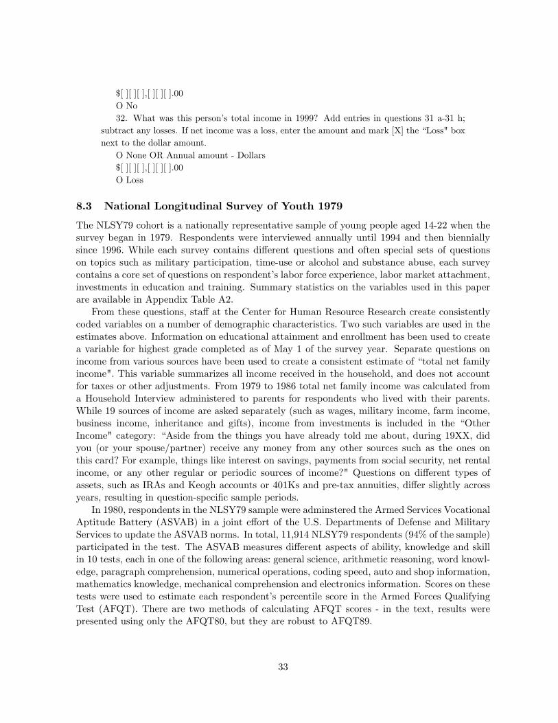
$[ ][ ][ ],[ ][ ][ ].00O No32. What was this person�s total income in 1999? Add entries in questions 31 a-31 h;

subtract any losses. If net income was a loss, enter the amount and mark [X] the �Loss" boxnext to the dollar amount.

O None OR Annual amount - Dollars$[ ][ ][ ],[ ][ ][ ].00O Loss

8.3 National Longitudinal Survey of Youth 1979

The NLSY79 cohort is a nationally representative sample of young people aged 14-22 when thesurvey began in 1979. Respondents were interviewed annually until 1994 and then bienniallysince 1996. While each survey contains di¤erent questions and often special sets of questionson topics such as military participation, time-use or alcohol and substance abuse, each surveycontains a core set of questions on respondent�s labor force experience, labor market attachment,investments in education and training. Summary statistics on the variables used in this paperare available in Appendix Table A2.

From these questions, sta¤ at the Center for Human Resource Research create consistentlycoded variables on a number of demographic characteristics. Two such variables are used in theestimates above. Information on educational attainment and enrollment has been used to createa variable for highest grade completed as of May 1 of the survey year. Separate questions onincome from various sources have been used to create a consistent estimate of �total net familyincome". This variable summarizes all income received in the household, and does not accountfor taxes or other adjustments. From 1979 to 1986 total net family income was calculated froma Household Interview administered to parents for respondents who lived with their parents.While 19 sources of income are asked separately (such as wages, military income, farm income,business income, inheritance and gifts), income from investments is included in the �OtherIncome" category: �Aside from the things you have already told me about, during 19XX, didyou (or your spouse/partner) receive any money from any other sources such as the ones onthis card? For example, things like interest on savings, payments from social security, net rentalincome, or any other regular or periodic sources of income?" Questions on di¤erent types ofassets, such as IRAs and Keogh accounts or 401Ks and pre-tax annuities, di¤er slightly acrossyears, resulting in question-speci�c sample periods.

In 1980, respondents in the NLSY79 sample were adminstered the Armed Services VocationalAptitude Battery (ASVAB) in a joint e¤ort of the U.S. Departments of Defense and MilitaryServices to update the ASVAB norms. In total, 11,914 NLSY79 respondents (94% of the sample)participated in the test. The ASVAB measures di¤erent aspects of ability, knowledge and skillin 10 tests, each in one of the following areas: general science, arithmetic reasoning, word knowl-edge, paragraph comprehension, numerical operations, coding speed, auto and shop information,mathematics knowledge, mechanical comprehension and electronics information. Scores on thesetests were used to estimate each respondent�s percentile score in the Armed Forces QualifyingTest (AFQT). There are two methods of calculating AFQT scores - in the text, results werepresented using only the AFQT80, but they are robust to AFQT89.

33

Dependent Variable:Sample:

Panel A: Any Income from AssetYears of schooling 3.60 *** 1.16 *** 2.00 *** 2.22 ***

(0.01) (0.01) (0.02) (0.03)

Num of Observations 10342137 1174130 4745546 475297R-Squared 0.142 0.071 0.163 0.121

Panel B: Amount of Income from AssetYears of schooling 273.23 *** 38.79 *** 510.77 *** 426.82 ***

(5.04) (0.98) (4.54) (6.29)

Num of Observations 10342137 1174130 4745546 475297R-Squared 0.088 0.019 0.141 0.113

Panel C: Percentile of Amount/Income in DistributionYears of schooling 342.53 *** 108.19 *** 202.87 *** 232.24 ***

(1.38) (1.34) (1.86) (2.92)

Num of Observations 9497305 1057689 4366472 431653R-Squared 0.128 0.063 0.171 0.139

Note: Standard errors are clustered by state of birth X year of birth. Data from the 1990 and 2000 census are used. This sample contains only 36-75 year olds (50-75 year olds when considering retirement income) and includes both men and women. Other controls include fixed effects for gender, 3-year age groups, 10-year birth cohorts, state of birth, state of residence and a cubic polynomial in earned income. Regressions for blacks also include state of residence fixed effects interacted with a dummy variable for being born in the South and turning age 14 in 1958 or later to account for the impact of Brown v. Board of Education. Top-coded individuals (those with income from investments greater than $50,000 or retirement income greater than $52,000) are dropped.

Whites Blacks(3) (4)

Table 1: OLS Estimates of the Effect of Schooling on Income from Various Sources

(1) (2)Blacks

Income from Retirement SavingsIncome from InvestmentsWhites

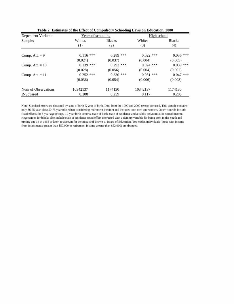
Dependent Variable:Sample:

Comp. Att. = 9 0.116 *** 0.289 *** 0.022 *** 0.036 ***(0.024) (0.037) (0.004) (0.005)

Comp. Att. = 10 0.139 *** 0.293 *** 0.024 *** 0.039 ***(0.028) (0.056) (0.004) (0.007)

Comp. Att. = 11 0.252 *** 0.330 *** 0.051 *** 0.047 ***(0.036) (0.054) (0.006) (0.008)

Num of Observations 10342137 1174130 10342137 1174130R-Squared 0.188 0.259 0.117 0.208

Note: Standard errors are clustered by state of birth X year of birth. Data from the 1990 and 2000 census are used. This sample contains only 36-75 year olds (50-75 year olds when considering retirement income) and includes both men and women. Other controls include fixed effects for 3-year age groups, 10-year birth cohorts, state of birth, state of residence and a cublic polynomial in earned income. Regressions for blacks also include state of residence fixed effect interacted with a dummy variable for being born in the South and turning age 14 in 1958 or later, to account for the impact of Brown v. Board of Education. Top-coded individuals (those with income from investments greater than $50,000 or retirement income greater than $52,000) are dropped.

High school

(3) (4)(1) (2)

Table 2: Estimates of the Effect of Compulsory Schooling Laws on Education, 2000Years of schooling

Whites BlacksWhites Blacks

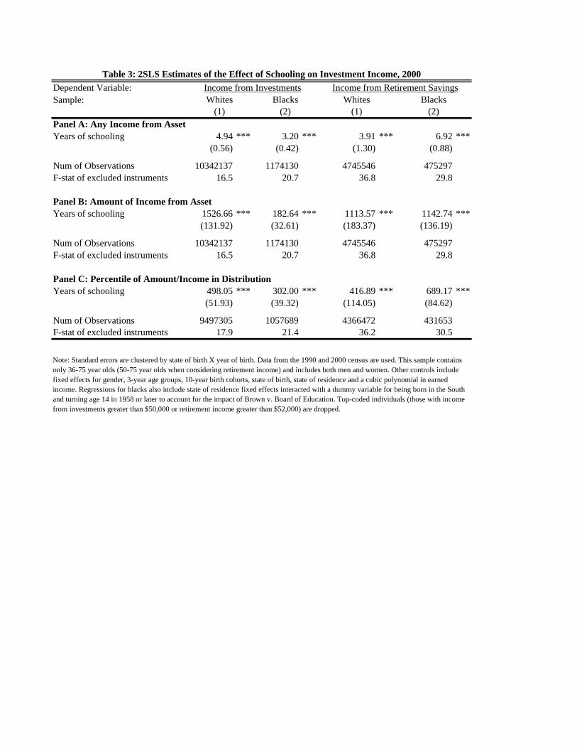
Dependent Variable:Sample:

Panel A: Any Income from AssetYears of schooling 4.94 *** 3.20 *** 3.91 *** 6.92 ***

(0.56) (0.42) (1.30) (0.88)

Num of Observations 10342137 1174130 4745546 475297F-stat of excluded instruments 16.5 20.7 36.8 29.8

Panel B: Amount of Income from AssetYears of schooling 1526.66 *** 182.64 *** 1113.57 *** 1142.74 ***

(131.92) (32.61) (183.37) (136.19)

Num of Observations 10342137 1174130 4745546 475297F-stat of excluded instruments 16.5 20.7 36.8 29.8

Panel C: Percentile of Amount/Income in DistributionYears of schooling 498.05 *** 302.00 *** 416.89 *** 689.17 ***

(51.93) (39.32) (114.05) (84.62)

Num of Observations 9497305 1057689 4366472 431653F-stat of excluded instruments 17.9 21.4 36.2 30.5

Note: Standard errors are clustered by state of birth X year of birth. Data from the 1990 and 2000 census are used. This sample contains only 36-75 year olds (50-75 year olds when considering retirement income) and includes both men and women. Other controls include fixed effects for gender, 3-year age groups, 10-year birth cohorts, state of birth, state of residence and a cubic polynomial in earned income. Regressions for blacks also include state of residence fixed effects interacted with a dummy variable for being born in the South and turning age 14 in 1958 or later to account for the impact of Brown v. Board of Education. Top-coded individuals (those with income from investments greater than $50,000 or retirement income greater than $52,000) are dropped.

Whites Blacks(1) (2)

Table 3: 2SLS Estimates of the Effect of Schooling on Investment Income, 2000

(2)

Income from Investments Income from Retirement Savings

(1)Whites Blacks

Dependent Variable Savings Percentile Inv. Income Inv. Income Percentile

Estimation Technique OLS OLS Probit OLS OLS(2) (3) (4) (5) (6)

State ever imposed mandate -1.25 -1.90 *** -0.07 *** -122.93 *** -178.76 ***(1.59) (0.38) (0.02) (22.50) (27.99)

Years since mandate 0.80 ** 0.33 *** 0.01 *** 18.95 *** 34.47 ***(0.35) (0.06) (0.00) (3.77) (4.65)

Married 3.18 ** -0.83 *** -0.02 *** -88.77 *** 476.25 ***(1.40) (0.06) (0.00) (11.19) (7.22)

College Educated 9.28 *** 12.38 *** 0.50 *** 930.95 *** 1070.64 ***(1.36) (0.09) (0.00) (21.27) (8.12)

Age 0.17 0.62 *** 0.02 *** 66.70 *** 59.05 ***(0.12) (0.02) (0.00) (2.53) (2.09)

Total Earnings/10^5 5.65 *** 37.00 *** 1.17 *** 2139.50 *** -460.70 ***(1.04) (0.16) (0.01) (33.84) (31.24)

R^2 0.11 0.01 0.02N 1,869 3,601,777 3,601,777 3,579,595 3,601,777

Table 4: BGM Results and Replication Using Census Data

Note: Columns (1) and (2) reproduce columns (1) and (2) from Table 5 of Bernheim, Garret, and Maki (2001), which used data from a 1995 telephone survey of individuals. The dependent variable is savings rate in column (1), and the households location in the national distribution of savings rates in column (2). Columns (3)-(6) replicate this approach, using data from the 2000 U.S. census. The dependent variable in column (3) and (4) is a dummy variable indicating whether the individual reported receiving any investment income. The dependent variable in column (5) is the level of investment income received, and in (6) is the individual's percentile ranking in the nationwide investment income distribution.

Census ReplicationAny Savings Income

BGM Original Result

Any Investment InvestmentInvestment Income Income

Income Percentile(1) (2) (3)

5 Years Prior 1.15 *** 152.17 * 100.16 ***(0.28) (77.81) (26.88)

4 Years Prior 1.01 *** 90.92 ** 78.42 ***(0.33) (44.79) (29.14)

3 Years Prior 1.12 *** 68.72 80.05 ***(0.14) (55.00) (13.91)

2 Years Prior 1.16 *** 111.13 ** 67.67 **(0.23) (49.35) (26.59)

1 Year Prior 1.18 *** 53.04 84.18 ***(0.19) (38.55) (20.03)

First Affected 1.13 *** 116.26 *** 63.29 ***(0.17) (33.94) (19.61)

1 Year Post 1.19 *** 151.74 *** 62.80 ***(0.20) (34.70) (18.83)

2 Years Post 0.95 *** 115.47 *** 41.31 *(0.22) (44.35) (21.40)

3 Years Post 1.34 *** 161.27 *** 88.76 ***(0.34) (43.89) (28.07)

4 Years Post 1.11 *** 246.64 *** 59.74 **(0.26) (46.04) (26.96)

5 Years or More 0.29 68.10 0.43(0.30) (50.09) (27.70)

N 3,579,595 3,579,595 3,579,595

Test of Prior vs. PostF-Statistic 0.04 9.51 0.91p-value 0.85 0.00 0.34

Table 5: Estimates of the Causal Effect of Financial Literacy Training

Note: This table describes the evolution of financial market participation prior to, and following, the imposition of mandated financial education in high schools. The dependent variable in column (1) is a dummy for whether the household reported any investment income; in column (2), it is the amount of investment income received; and in column (3) it is the individual's percentile ranking in the nationwide investment income distribution. Additional controls include sex and marital status, birthyear dummies, educational attainment dummies, and a cubic control for income.The last two lines of the table test whether the average value of the dummy variables indicating the years four, three, two, and one year prior to the imposition of mandates are equal to those indicating the years one, two, three and four years following the mandate.

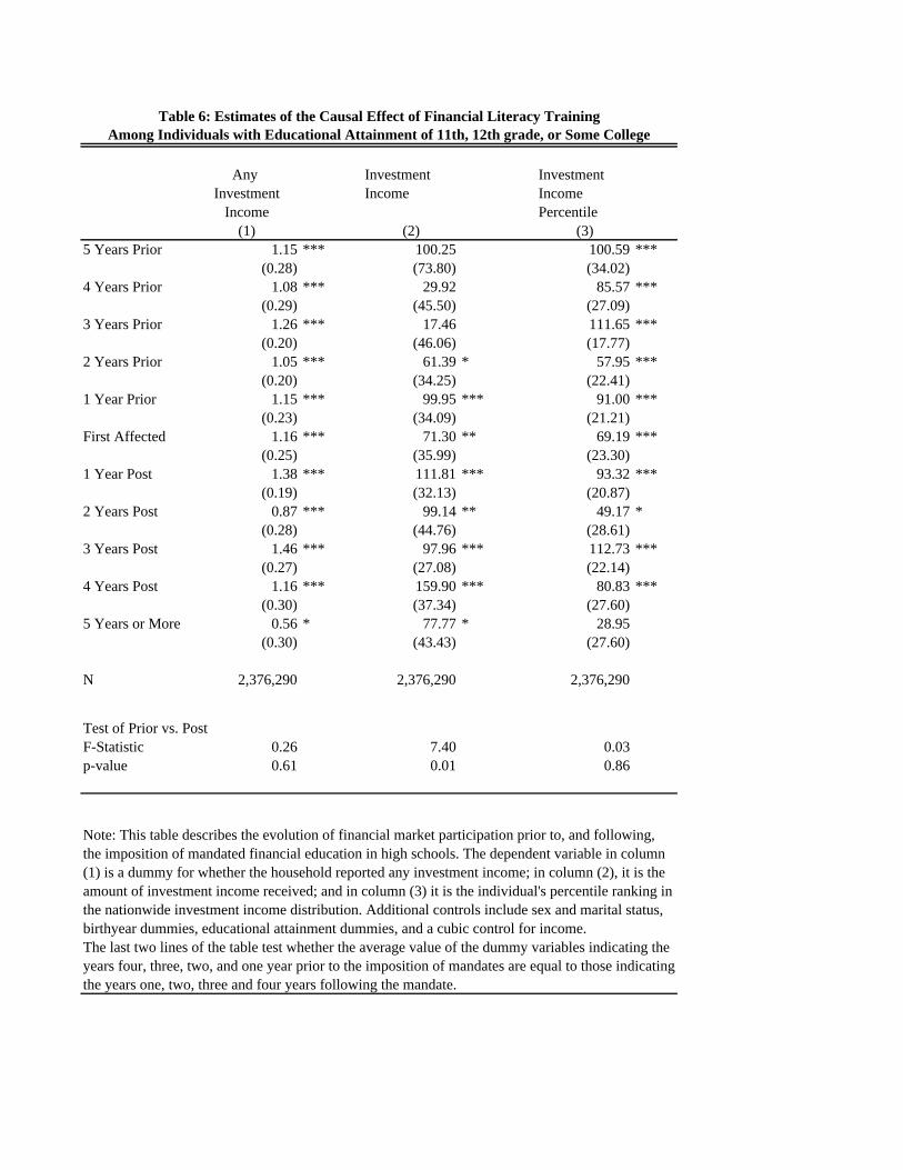
Any Investment InvestmentInvestment Income Income

Income Percentile(1) (2) (3)

5 Years Prior 1.15 *** 100.25 100.59 ***(0.28) (73.80) (34.02)

4 Years Prior 1.08 *** 29.92 85.57 ***(0.29) (45.50) (27.09)

3 Years Prior 1.26 *** 17.46 111.65 ***(0.20) (46.06) (17.77)

2 Years Prior 1.05 *** 61.39 * 57.95 ***(0.20) (34.25) (22.41)

1 Year Prior 1.15 *** 99.95 *** 91.00 ***(0.23) (34.09) (21.21)

First Affected 1.16 *** 71.30 ** 69.19 ***(0.25) (35.99) (23.30)

1 Year Post 1.38 *** 111.81 *** 93.32 ***(0.19) (32.13) (20.87)

2 Years Post 0.87 *** 99.14 ** 49.17 *(0.28) (44.76) (28.61)

3 Years Post 1.46 *** 97.96 *** 112.73 ***(0.27) (27.08) (22.14)

4 Years Post 1.16 *** 159.90 *** 80.83 ***(0.30) (37.34) (27.60)

5 Years or More 0.56 * 77.77 * 28.95(0.30) (43.43) (27.60)

N 2,376,290 2,376,290 2,376,290

Test of Prior vs. PostF-Statistic 0.26 7.40 0.03p-value 0.61 0.01 0.86

Note: This table describes the evolution of financial market participation prior to, and following, the imposition of mandated financial education in high schools. The dependent variable in column (1) is a dummy for whether the household reported any investment income; in column (2), it is the amount of investment income received; and in column (3) it is the individual's percentile ranking in the nationwide investment income distribution. Additional controls include sex and marital status, birthyear dummies, educational attainment dummies, and a cubic control for income.The last two lines of the table test whether the average value of the dummy variables indicating the years four, three, two, and one year prior to the imposition of mandates are equal to those indicating the years one, two, three and four years following the mandate.

Table 6: Estimates of the Causal Effect of Financial Literacy TrainingAmong Individuals with Educational Attainment of 11th, 12th grade, or Some College

Log Log Log Log LogGDP GDP GDP GDP GDP

Growth Growth Growth Growth Growth(1) (2) (2) (2) (2)

5 Years Prior 0.480 *** 0.394 *** 0.433 *** 0.290 *** 0.207 *(0.105) (0.102) (0.108) (0.096) (0.109)

4 Years Prior 0.240 ** 0.168 * 0.196 * 0.083 0.092(0.112) (0.098) (0.119) (0.096) (0.099)

3 Years Prior 0.208 ** 0.136 0.175 * 0.041 0.007(0.100) (0.095) (0.105) (0.091) (0.063)

2 Years Prior 0.186 * 0.114 0.165 * 0.015 -0.062(0.096) (0.096) (0.098) (0.092) (0.072)

1 Year Prior 0.206 ** 0.134 0.197 ** 0.037 -0.073(0.090) (0.091) (0.097) (0.085) (0.066)

Law Passed 0.196 0.124 0.198 0.033 -0.070(0.128) (0.135) (0.131) (0.126) (0.080)

1 Year Post 0.242 ** 0.170 0.256 ** 0.091 0.067(0.105) (0.115) (0.111) (0.116) (0.144)

2 Years Post 0.274 ** 0.202 0.299 ** 0.140 0.072(0.122) (0.123) (0.131) (0.127) (0.101)

3 Years Post 0.107 0.035 0.144 -0.005 -0.028(0.125) (0.128) (0.124) (0.112) (0.088)

4 Years Post -0.124 -0.196 -0.075 -0.207 * -0.105(0.118) (0.123) (0.113) (0.108) (0.078)

5 Years or More -0.205 *** -0.265 *** -0.101 -0.059 -0.062(0.059) (0.061) (0.063) (0.057) (0.057)

R2 0.05 0.14 0.08 0.27 0.49N 1,296 1,296 1,296 1,296 1,296

P-value from F-Test of: 5 Years Prior - 1 Year Prior 0.00 0.00 0.00 0.02 0.20 1 Year Post - 5+ Years Post 0.03 0.00 0.14 0.32 0.51 All Treatment Dummies 0.00 0.00 0.00 0.00 0.00

State Fixed Effects No Yes Yes Yes YesYear Controls None None Linear Cubic Fixed Effects

Table 7: State GDP Growth and Passage of Financial Literacy Education Requirements

Note: This table describes the evolution of state GDP growth prior to, and following, the imposition of mandated financial education in high schools. The dependent variable in each column is 100*(log(gdpt/gdpt-1)). Standard errors are clustered at the state level. Columns (2)-(5) include state fixed effects. Column (3) includes a linear time trend, Column (4) a cubic polynomial, and Column (5) year fixed effects.

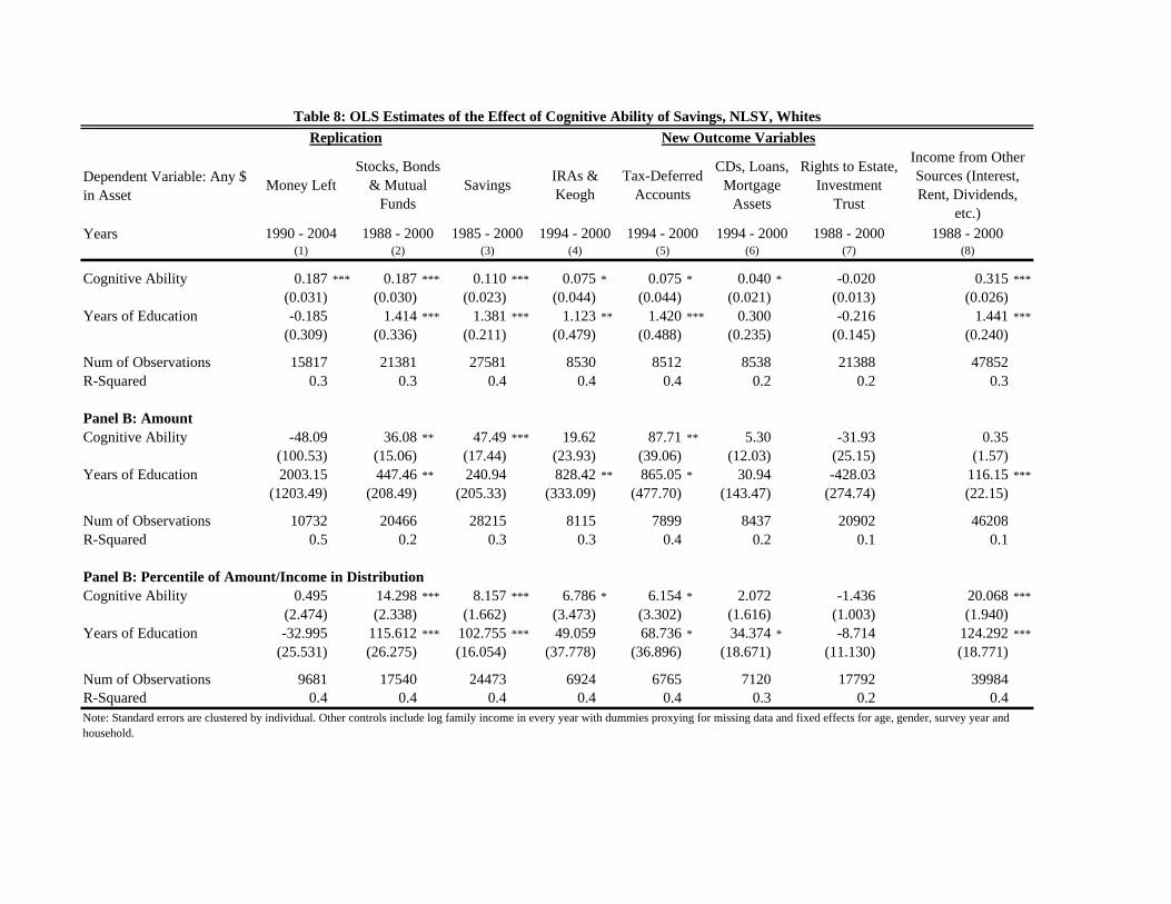
Dependent Variable: Any $ in Asset

Years

Cognitive Ability 0.187 *** 0.187 *** 0.110 *** 0.075 * 0.075 * 0.040 * -0.020 0.315 ***(0.031) (0.030) (0.023) (0.044) (0.044) (0.021) (0.013) (0.026)

Years of Education -0.185 1.414 *** 1.381 *** 1.123 ** 1.420 *** 0.300 -0.216 1.441 ***(0.309) (0.336) (0.211) (0.479) (0.488) (0.235) (0.145) (0.240)

Num of Observations 15817 21381 27581 8530 8512 8538 21388 47852R-Squared 0.3 0.3 0.4 0.4 0.4 0.2 0.2 0.3

Panel B: AmountCognitive Ability -48.09 36.08 ** 47.49 *** 19.62 87.71 ** 5.30 -31.93 0.35

(100.53) (15.06) (17.44) (23.93) (39.06) (12.03) (25.15) (1.57)Years of Education 2003.15 447.46 ** 240.94 828.42 ** 865.05 * 30.94 -428.03 116.15 ***

(1203.49) (208.49) (205.33) (333.09) (477.70) (143.47) (274.74) (22.15)

Num of Observations 10732 20466 28215 8115 7899 8437 20902 46208R-Squared 0.5 0.2 0.3 0.3 0.4 0.2 0.1 0.1

Panel B: Percentile of Amount/Income in DistributionCognitive Ability 0.495 14.298 *** 8.157 *** 6.786 * 6.154 * 2.072 -1.436 20.068 ***

(2.474) (2.338) (1.662) (3.473) (3.302) (1.616) (1.003) (1.940)Years of Education -32.995 115.612 *** 102.755 *** 49.059 68.736 * 34.374 * -8.714 124.292 ***

(25.531) (26.275) (16.054) (37.778) (36.896) (18.671) (11.130) (18.771)

Num of Observations 9681 17540 24473 6924 6765 7120 17792 39984R-Squared 0.4 0.4 0.4 0.4 0.4 0.3 0.2 0.4Note: Standard errors are clustered by individual. Other controls include log family income in every year with dummies proxying for missing data and fixed effects for age, gender, survey year and household.

1988 - 2000(1) (2) (3) (4) (5) (6) (7) (8)

1985 - 2000 1994 - 2000

Tax-Deferred Accounts

IRAs & Keogh

Table 8: OLS Estimates of the Effect of Cognitive Ability of Savings, NLSY, WhitesReplication New Outcome Variables

Income from Other Sources (Interest, Rent, Dividends,

etc.)1994 - 20001994 - 2000 1988 - 2000

Money Left SavingsCDs, Loans,

Mortgage Assets

Rights to Estate, Investment

Trust

1988 - 2000

Stocks, Bonds & Mutual

Funds

1990 - 2004

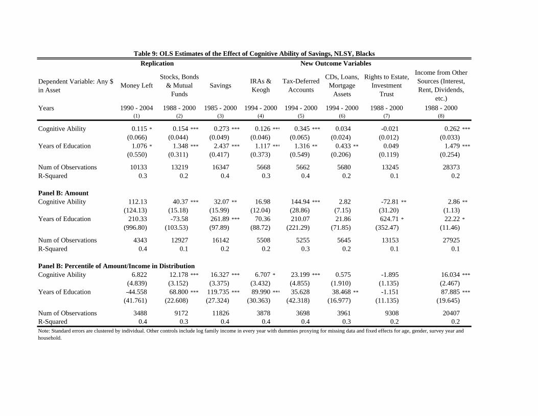
Dependent Variable: Any $ in Asset

Years

Cognitive Ability 0.115 * 0.154 *** 0.273 *** 0.126 *** 0.345 *** 0.034 -0.021 0.262 ***(0.066) (0.044) (0.049) (0.046) (0.065) (0.024) (0.012) (0.033)

Years of Education 1.076 * 1.348 *** 2.437 *** 1.117 *** 1.316 ** 0.433 ** 0.049 1.479 ***(0.550) (0.311) (0.417) (0.373) (0.549) (0.206) (0.119) (0.254)

Num of Observations 10133 13219 16347 5668 5662 5680 13245 28373R-Squared 0.3 0.2 0.4 0.3 0.4 0.2 0.1 0.2

Panel B: AmountCognitive Ability 112.13 40.37 *** 32.07 ** 16.98 144.94 *** 2.82 -72.81 ** 2.86 **

(124.13) (15.18) (15.99) (12.04) (28.86) (7.15) (31.20) (1.13)Years of Education 210.33 -73.58 261.89 *** 70.36 210.07 21.86 624.71 * 22.22 *

(996.80) (103.53) (97.89) (88.72) (221.29) (71.85) (352.47) (11.46)

Num of Observations 4343 12927 16142 5508 5255 5645 13153 27925R-Squared 0.4 0.1 0.2 0.2 0.3 0.2 0.1 0.1

Panel B: Percentile of Amount/Income in DistributionCognitive Ability 6.822 12.178 *** 16.327 *** 6.707 * 23.199 *** 0.575 -1.895 16.034 ***

(4.839) (3.152) (3.375) (3.432) (4.855) (1.910) (1.135) (2.467)Years of Education -44.558 68.800 *** 119.735 *** 89.990 *** 35.628 38.468 ** -1.151 87.885 ***

(41.761) (22.608) (27.324) (30.363) (42.318) (16.977) (11.135) (19.645)

Num of Observations 3488 9172 11826 3878 3698 3961 9308 20407R-Squared 0.4 0.3 0.4 0.4 0.4 0.3 0.2 0.2Note: Standard errors are clustered by individual. Other controls include log family income in every year with dummies proxying for missing data and fixed effects for age, gender, survey year and household.

(5) (6) (7) (8)(1) (2) (3) (4)1994 - 20001994 - 2000

New Outcome VariablesIncome from Other Sources (Interest, Rent, Dividends,

etc.)1988 - 2000

Tax-Deferred Accounts

IRAs & Keogh

1988 - 2000

CDs, Loans, Mortgage

Assets

Table 9: OLS Estimates of the Effect of Cognitive Ability of Savings, NLSY, BlacksReplication

Rights to Estate, Investment

Trust

1988 - 2000

Stocks, Bonds & Mutual

Funds

1990 - 2004 1985 - 2000

Money Left Savings

1994 - 2000

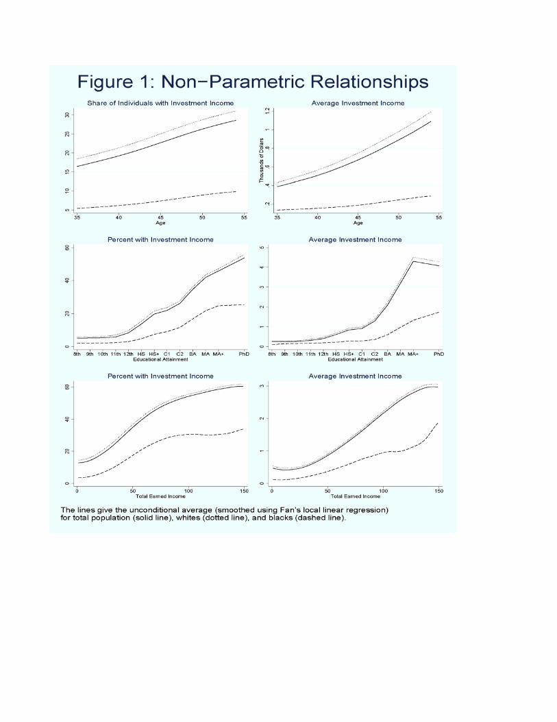
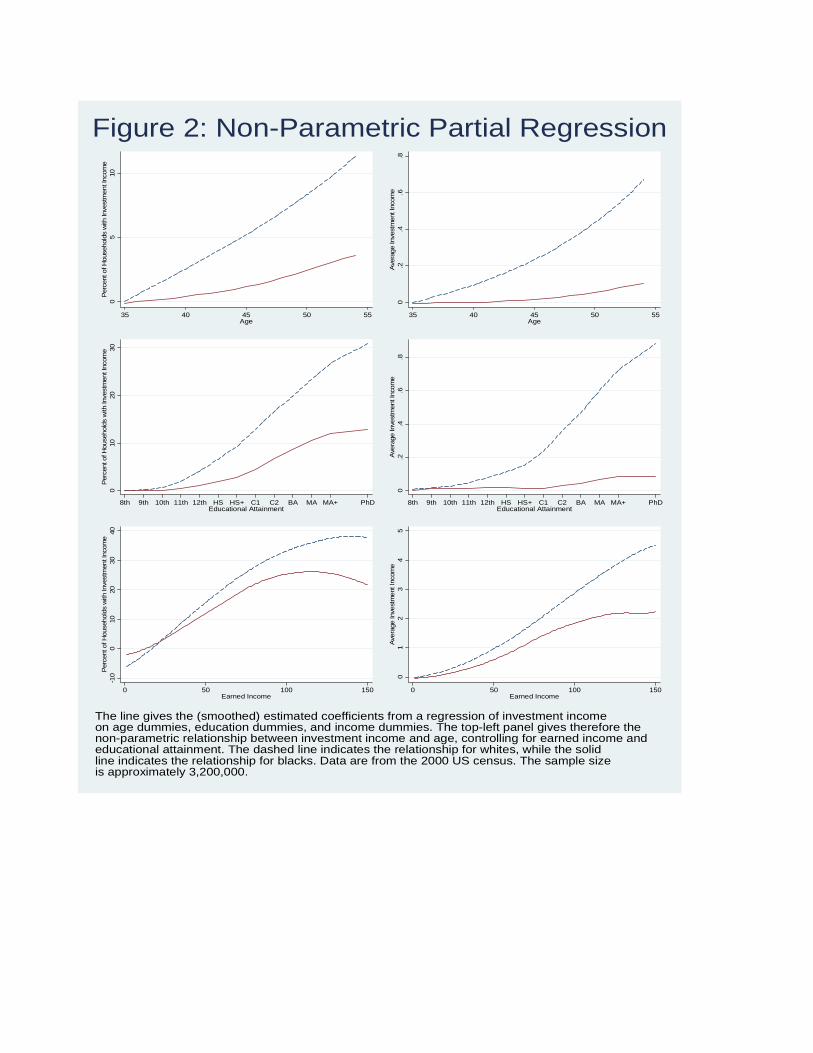
05

10P

erce

nt o

f Hou

seho

lds

with

Inve

stm

ent I

ncom

e

35 40 45 50 55Age

0.2

.4.6

.8A

vera

ge In

vest

men

t Inc

ome

35 40 45 50 55Age

010

2030

Per

cent

of H

ouse

hold

s w

ith In

vest

men

t Inc

ome

8th 9th 10th 11th 12th HS HS+ C1 C2 BA MA MA+ PhDEducational Attainment

0.2

.4.6

.8A

vera

ge In

vest

men

t Inc

ome

8th 9th 10th 11th 12th HS HS+ C1 C2 BA MA MA+ PhDEducational Attainment

-10

010

2030

40P

erce

nt o

f Hou

seho

lds

with

Inve

stm

ent I

ncom

e

0 50 100 150Earned Income

01

23

45

Ave

rage

Inve

stm

ent I

ncom

e

0 50 100 150Earned Income

The line gives the (smoothed) estimated coefficients from a regression of investment incomeon age dummies, education dummies, and income dummies. The top-left panel gives therefore thenon-parametric relationship between investment income and age, controlling for earned income andeducational attainment. The dashed line indicates the relationship for whites, while the solidline indicates the relationship for blacks. Data are from the 2000 US census. The sample sizeis approximately 3,200,000.

Figure 2: Non-Parametric Partial Regression

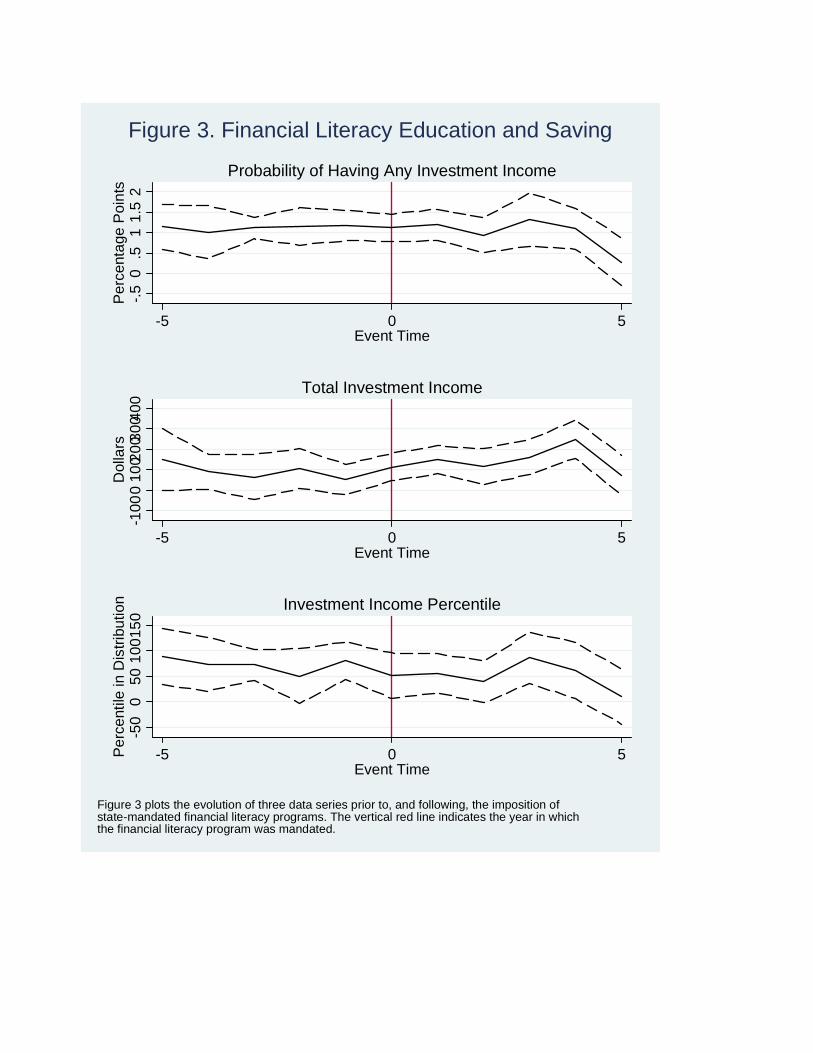
-.50

.51

1.5

2P

erce

ntag

e P

oint

s

-5 0 5Event Time

Probability of Having Any Investment Income

-100

010

0200

3004

00D

olla

rs

-5 0 5Event Time

Total Investment Income

-50

050

1001

50Pe

rcen

tile

in D

istri

butio

n

-5 0 5Event Time

Investment Income Percentile

Figure 3 plots the evolution of three data series prior to, and following, the imposition ofstate-mandated financial literacy programs. The vertical red line indicates the year in whichthe financial literacy program was mandated.

Figure 3. Financial Literacy Education and Saving

Variable Mean St. Dev. Mean St. Dev. Mean St. Dev.(1) (2) (3) (4) (5) (6)

Years of schooling 13.19 2.62 13.29 2.55 12.32 3.04High school graduation 0.85 0.36 0.86 0.35 0.73 0.44Comp. Att. = 9 0.40 0.49 0.39 0.49 0.44 0.50Comp. Att. = 10 0.11 0.31 0.11 0.31 0.10 0.31Comp. Att. = 11 0.36 0.48 0.37 0.48 0.30 0.46Age 48.89 13.05 49.05 13.07 47.53 12.73Male 0.48 0.50 0.48 0.50 0.44 0.50Black 0.10 0.30

Income from InvestmentsAny 28.23 45.01 30.50 46.04 8.16 27.37Amount 1302.94 4659.14 1424.17 4861.49 235.06 1862.55Percentile 2592.18 3912.44 2797.65 3995.98 747.16 2364.69

Income from Retirement SavingsAny 10.85 31.11 11.00 31.28 9.61 29.47Amount 1278.628 4928.848 1310.17 5005.48 999.33 4179.30Percentile 1109.67 3029.51 1120.98 3041.38 1007.63 2918.11

Whites BlacksAppendix Table A1: Summary Statistics, Census

Whole Sample

Variable Year(s) Mean St. Dev. Mean St. Dev.(1) (2) (3) (4) (5)

Cognitive Ability 1981 48.70 28.42 19.96 18.24Years of Education 1985 - 2004 13.35 2.47 12.62 2.01Age (in year 1979) 1979 17.14 2.08 17.23 2.04Male 1979 0.51 0.50 0.52 0.50Total Net Family Income 1979 - 2004 60964.86 99865.25 35461.28 51636.37Pearlin "Little Control Over Life" 1992 1.74 0.62 1.85 0.70

Any …Money Left 1990 - 2004 77.96 41.45 48.68 49.99Savings 1985 - 2000 75.77 42.85 46.68 49.89Stocks, Bonds & Mutual Funds 1988 - 2000 23.79 42.58 7.76 26.76IRAs & Keogh 1994 - 2000 29.31 45.52 8.24 27.50Tax-Deferred Accounts 1994 - 2000 41.03 49.19 22.57 41.81CDs, Loans, Mortgage Assets 1994 - 2000 7.19 25.83 2.50 15.61Rights to Estate, Investment Trust 1988 - 2000 4.60 20.95 1.63 12.66Income from Other Sources 1979 - 2002 43.09 49.52 12.74 33.34

Amount …Money Left 1990 - 2004 84145 115436 28523 59001Savings 1985 - 2000 9807 30028 2465 11992Stocks, Bonds & Mutual Funds 1988 - 2000 4281 25528 656 9119IRAs & Keogh 1994 - 2000 7692 30866 1002 8392Tax-Deferred Accounts 1994 - 2000 15077 43346 3186 16432CDs, Loans, Mortgage Assets 1994 - 2000 1472 13165 332 5396Rights to Estate, Investment Trust 1988 - 2000 3410 52389 879 22888Income from Other Sources 1979 - 2002 743 4176 172 1576

Percentile …Money Left 1990 - 2004 4720 2413 3140 2328Savings 1985 - 2000 4347 2751 2553 2761Stocks, Bonds & Mutual Funds 1988 - 2000 1654 3102 522 1892IRAs & Keogh 1994 - 2000 1985 3250 508 1843Tax-Deferred Accounts 1994 - 2000 2670 3388 1352 2681CDs, Loans, Mortgage Assets 1994 - 2000 485 1877 167 1123Rights to Estate, Investment Trust 1988 - 2000 261 1410 96 863Income from Other Sources 1979 - 2002 2996 3465 910 2350

Whites BlacksAppendix Table A2: Summary Statistics, NLSY

Appendix Table A3: Comparison of Data from 2001 SCF and 2000 Census

Investment Income Any Investment Income Retirement Income Any Retirement IncomeSCF Census SCF Census SCF Census SCF Census

Mean 1515 1264 0.33 0.27 4114 2866 0.27 0.22Standard Deviation 5089 4543 0.47 0.45 9545 7477 0.44 0.41Min 0 0 0 0 0 0 0 0Max 49800 49900 1 1 50400 51000 1 1

Percentiles1% 0 0 0 0 0 0 0 0

10% 0 0 0 0 0 0 0 025% 0 0 0 0 0 0 0 0

Median 0 0 0 0 0 0 0 075% 200 50 1 1 1320 0 1 090% 3500 2900 1 1 15600 11165 1 199% 29000 25000 1 1 43200 36539 1 1

N 2,720 5,427,616 2,735 5,450,827 1,739 2,883,474 1,739 2,883,474

Note: This table compares the means, standard deviations, and percentiles for the key variables, using data from both the Census and the Survey of Consumer Finances. The Census data are from the 2000 census, while the SCF data are from the 2001 survey of consumer finances. The sample for investment income vairables in both surveys is adults aged 36-75 who report investment income below $50,000. For retirement income, the sample is individuals aged 50 to 75 who report retirement income less than or equal to $52,000. N indicates the number of unique individuals used to estimate numbers; for the SCF, appropriate weights were used.

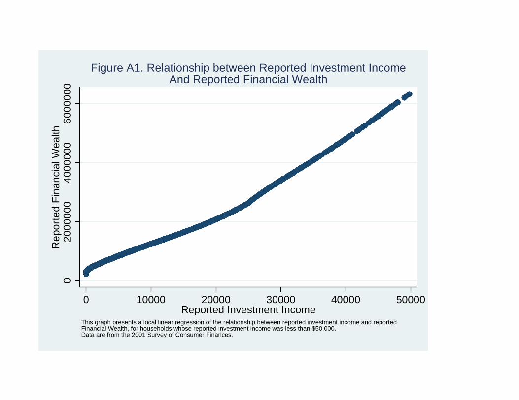
020

0000

040

0000

060

0000

0R

epor

ted

Fina

ncia

l Wea

lth

0 10000 20000 30000 40000 50000Reported Investment Income

This graph presents a local linear regression of the relationship between reported investment income and reported Financial Wealth, for households whose reported investment income was less than $50,000.Data are from the 2001 Survey of Consumer Finances.

Figure A1. Relationship between Reported Investment IncomeAnd Reported Financial Wealth