IENG581

Design and Analysis of Experiments

INTRODUCTION

Experimental Design

Experiments are performed by investigators in virtually all fields of inquiry,

usually to discover something about a particular process or system.

Experiment is a test.

Designed experiment is a test or series of tests in which purposeful

changes are made to the input variables of a process or system so that

we may observe and identify the reasons for changes in the output

response.

The process or system under study can be represented by the model shown

in the figure below:

Figure: General model of a process or system

We can visualize the process as a combination of machines, methods,

people, and other resources that transforms some input (often a material)

into an output that has one or more observable responses.

Some of the process variables x1,x2,…,xp are controllable, whereas other

variables z1,z2,…,zq are uncontrollable (although they may be controllable

for purposes of a test).

The objectives of the experiment may include the following:

1. Determining which variables are most influential on the response y

2. Determining where to set the influential x’s so that y is almost always

near the desired nominal value

3. Determining where to set the influential x’s so that variability in y is

small.

4. Determining where to set the influential x’s so that the effects of the

uncontrollable variables z1,z2,…,zq are minimized.

Experimental design methods play an important role in process

development and process troubleshooting to improve performance.

The objective in many cases may be to develop a robust process, that is, a

process affected minimally by external sources of variability (the z’s).

*In any experiment, the results and conclusions that can be drawn depend

to a large extent on the manner in which the data were collected.

Applications of Experimental Design:

Experimental design methods, have found broad application in many

disciplines. In fact we may view experimentation as part of the scientific

process and as one of the ways we learn about how systems or processes

work.

Generally, we learn through a series of activities in which we make

conjectures about a process, perform experiments to generate data from

the process, and then use the information from the experiment to

establish new conjectures, which lead to new experiments, and so on.

Experimental design is a critically important tool in the engineering

world for improving the performance of a manufacturing process.

It also has extensive application in the development of new processes.

The application of experimental design techniques early in process

development can result in:

1. Improved process yields

2. Reduced variability and closer conformance to nominal or target

requirements.

3. Reduced development time.

4. Reduced overall costs.

Experimental design also plays a major role in engineering design

activities, where new products are developed and existing ones are

improved.

Some applications of Experimental design are:

1. Evaluation and comparison of basic design configurations.

2. Evaluation of material alterations.

3. Selection of design parameters so that the product will work well

under a wide variety of field conditions, that is, so that the product is

robust.

4. Determination of key product design parameters that impact product

performance.

The use of experimental design in these areas can result in:

- products that are easier to manufacture,

- products that have enhanced field performance and reliability,

- lower product cost,

- and shorter product design and development time.

Basic Principles of Experimental Design

If any experiment is to be performed most efficiently, then a scientific

approach to planning the experiments must be employed.

By the statistical design of experiments, we refer to the process of planning

the experiment so that appropriate data that can be analyzed by statistical

methods will be collected, resulting in valid and objective conclusions.

*The statistical approach to experimental design is necessary if we wish to

draw meaningful conclusions from the data.

When the problem involves data that are subject to experimental errors,

statistical methodology is the only objective approach to analysis.

Thus, there are two aspects to any experimental problem:

- The design of the experiment and

- the statistical analysis of the data.

These two subjects are closely related since the method of analysis depends

directly on the design employed.

Both topics will be addresses in this course (IE-581).

The three basic principles of experimental design are:

- Replication,

- Randomization, and

- Blocking.

Replication has two important properties:

First, it allows the experimenter to obtain an estimate of the experimental

error. This estimate of error becomes a basic unit of measurement for

determining whether observed differences in the data are really statistically

different.

Second, if the sample mean (e.g. ÿ) is used to estimate the effect of a factor

in the experiment, then replication permits the experimenter to obtain a more

precise estimate of this effect.

e.g. If 2 is the variance of the data, and there are n replicates, then the

variance of the sample mean is:

2 ÿ = 2/n

- If n=1, the experimental error will be high and we will be unable to make

satisfactory inferences, since the observed difference in the sample mean

could be the result of experimental error.

- If n is reasonably large, the experimental error will be sufficient small and

we would be reasonably safe in conclusion.

Randomization is the cornerstone underlying the use of statistical

methods in experimental design.

By randomization we mean that both, the allocation of the experimental

material and the order in which the individual runs or trials of the

experiment are to be performed, are randomly determined.

Statistical methods require that the observations (or errors) be

independently distributed random variables. Randomization usually

makes this assumption valid.

By properly randomizing the experiment, we also assist in “averaging

out” the effects of extraneous factors that may be present.

Blocking is a technique used to increase the precision of an experiment.

A block is a portion of the experimental material that should be more

homogeneous than the entire set of material.

Blocking involves making comparisons among the conditions of interest

in the experiment within each block.

Guidelines for Designing Experiments:

To use the statistical approach in designing and analyzing, it is

necessary that everyone involved in the experiment have a clear idea in

advance of:

- Exactly what is to be studied,

- How the data are to be collected, and

- At least a qualitative understanding of how these data are to

be analyzed.

An outline of the recommended procedure is as follows:

1. Recognition and statement of the problem

In practice it is often not simple neither to realize that a problem requiring

experimentation exists, nor is it simple to develop a clear and generally

accepted statement of this problem.

It is necessary to develop all ideas about the objectives of the experiment.

Usually, it is important to solicit input from all concerned parties:

- Engineering,

- Quality assurance,

- Manufacturing,

- Marketing,

- Management,

- The customer, and operating personnel

- Etc….

A clear statement of the problem often contributes substantially to a

better understanding of the phenomena and the final solution of the

problem.

2. Choice of factors and levels

The experimenter must choose the factors to be varied in the experiment,

the ranges over which these factors will be varied, and the specific levels at

which runs will be made. Thought must also be given to how these factors

are to be controlled at the desired values and how they are to be

measured.

3. Selection of the response variable

In selecting the response variable, the experimenter should be certain

that this variable really provides useful information about the process

under study. Most often, the average or standard deviation (or both) of the

measured characteristic will be the response variable.

Multiple responses are not unusual.

4. Choice of experimental design

If the first three steps are done correctly, this step is relatively easy.

Choice of design involves:

- The consideration of sample size (number of replicates),

- The selection of a suitable run order for the experimental

trials,

- And the determination of whether or not blocking or other

randomization restrictions are involved.

In selecting the design, it is important to keep the experimental

objectives in mind.

5. Performing the experiment

When running the experiment, it is vital to monitor the process carefully

to ensure that everything is being done according to plan.

Errors in experimental procedure at this stage will usually destroy

experimental validity.

Up-front planning is crucial to success.

6. Data analysis

Statistical methods should be used to analyze the data so that results

and conclusions are objective rather than judgmental in nature.

If the experiment has been designed correctly and if it has been

performed according to the design, then the statistical methods required

are not elaborate.

There are many excellent software packages designed to assist in data

analysis, and simple graphical methods play an important role in data

interpretation.

Residual analysis and model adequacy checking are also important

analysis techniques.

Note: Remember that:

- Statistical methods cannot prove that a factor (or factors)

has a particular effect. They only provide guidelines as to

the reliability and validity of results.

- Properly applied, statistical methods do not allow anything

to be proved, experimentally, but they do allow us to

measure the likely error in a conclusion or to attach a level

of confidence to a statement.

- The primary advantage of statistical methods is that they

add objectivity to the decision-making process.

- Statistical techniques coupled with good engineering or

process knowledge and common sense will usually lead to

sound conclusions.

7. Conclusions and recommendations

Once the data have been analyzed,

- The experimenter must draw practical conclusions about the results

and recommend a course of action.

- Graphical methods are often useful in this stage, particularly in

presenting the results to others.

- Follow-up runs and confirmation testing should also be performed to

validate the conclusions from the experiment.

Throughout this entire process, it is important to keep in mind that

experimentation is an important part of the learning process, where;

- We tentatively formulate hypotheses about a system,

- Perform experiments to investigate these hypotheses, and

- On the basis of the results formulate new hypotheses, and so

on.

This suggests that experimentation is iterative.

Using statistical techniques in experimentation

Much of the research in engineering, science and industry is empirical

and makes extensive use of experimentation. Statistical methods can

greatly increase the efficiency of these experiments and often

strengthens the conclusions so obtained.

The intelligent use of statistical techniques in experimentation requires

that the experimenter keep the following points in mind:

1. Use your non-statistical knowledge of the problem.

2. Keep the design and analysis as simple as possible.

3. Recognize the difference between practical and statistical

significance.

4. Experiments are usually iterative

SIMPLE COMPARATIVE EXPERIMENTS

We’ll consider experiments to compare two conditions (sometimes called

treatments).

We’ll begin with an example of an experiment performed to determine

whether two different formulations of a product give equivalent results.

The discussion leads to a review of several basic statistical concepts.

Example:

The tension bond strength of Portland cement mortar is an important

characteristic of the product. An engineer is interested in comparing the

strength of a modified formulation in which polymer latex emulsions

have been added during mixing to the strength of the unmodified

mortar. The experimenter has collected 10 observations of strength for

the modified formulation and another 10 observations for the

unmodified formulation.

The data are shown in table 2-1.

We could refer to the two different formulations as two treatments or as

two levels of the factor formulations.

The data from this experiment are plotted in figure 2-1, below:

This display is called a dot diagram.

Visual examination of these data gives the immediate impression that

the strength of the unmodified mortar is greater than the strength of the

modified mortar. This impression is supported by comparing the

average tension bond strengths, Ÿ1=16.76 kgf/cm2 for the modified

mortar and Ÿ2=17.92 kgf/cm2 for the unmodified mortar.

The average tension bond strengths in these two samples differ by what

seems to be a nontrivial amount. However, it is not obvious that this

difference is large enough to imply that the two formulations really are

different.

Perhaps this observed difference in average strengths is the result of

sampling fluctuations and the two formulations are really identical.

Possibly another two samples would give opposite results, with the

strength of the modified mortar exceeding that of the unmodified

formulation.

A technique of statistical inference called hypothesis testing (or

significance testing) can be used to assist the experimenter in comparing

these two formulations.

Hypothesis testing allows the comparison of the two formulations to be

made on objective terms, with knowledge of the risks associated with

reaching the wrong conclusion.

To present procedures for hypothesis testing in simple comparative

experiments, however, it is first necessary to develop and review some

elementary statistical concepts.

2-2 Basic Statistical Concepts

Each of the observations in the Portland cement experiment described

previously would be called a run.

Notice that the individual runs differ, so there is fluctuation or noise in

the results.

This noise is usually called experimental error or simply error.

It is a statistical error, meaning that it arises from variation that is

uncontrolled and generally unavoidable.

The presence of error or noise implies that the response variable,

tension bond strength, is a random variable.

A random variable may be either discrete or continuous.

If the set of all possible values of the random variable is either

finite or countably infinite, then the random variable is discrete.

If the set of all possible values of the random variable is an

interval, then the random variable is continuous.

Graphical Description of variability

The Dot Diagram, illustrated in figure 2-1, is a very useful device for

displaying a small body of data.

The Dot Diagram enables the experimenter to see quickly the general

location or central tendency of the observations and their spread.

In our example; the Dot Diagram reveals that the two formulations

probably differ in mean strength but that both formulations produce

about the same variation in strength.

If the data is numerous, then a histogram may be preferable.

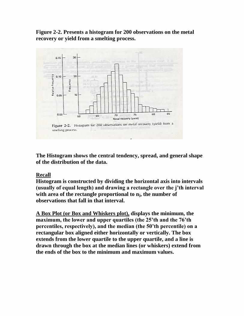
Figure 2-2. Presents a histogram for 200 observations on the metal

recovery or yield from a smelting process.

The Histogram shows the central tendency, spread, and general shape

of the distribution of the data.

Recall

Histogram is constructed by dividing the horizontal axis into intervals

(usually of equal length) and drawing a rectangle over the j’th interval

with area of the rectangle proportional to nj, the number of

observations that fall in that interval.

A Box Plot (or Box and Whiskers plot), displays the minimum, the

maximum, the lower and upper quartiles (the 25’th and the 76’th

percentiles, respectively), and the median (the 50’th percentile) on a

rectangular box aligned either horizontally or vertically. The box

extends from the lower quartile to the upper quartile, and a line is

drawn through the box at the median lines (or whiskers) extend from

the ends of the box to the minimum and maximum values.

Figure 2-3 presents the Box Plots for the two samples of tension bond

strength in the Portland cement mortar experiment.

This display clearly reveals the difference in mean strength between the

two formulations. It also indicates that both formulations produce

reasonably symmetric distributions of strength with similar variability

or spread.

Summary:

Dot diagrams, histograms, and Box plots are useful for summarizing the

information in a sample of data.

To describe the observations that might occur in a sample more

completely; we use the concept of the probability distribution.

Probability Distributions:

The probability structure of a random variable, say y, is described by its

probability distribution.

If y is discrete, we often call the probability distribution of y, say p(y),

the probability function of y.

If y is continuous, the probability distribution of y, say f(y), is often

called the probability density function for y.

The figures below, illustrate a hypothetical discrete and continuous

probability distributions.

Notice: In the discrete probability distribution, it is the height of the

function p(y) that represents probability, whereas in the continuous

case, it is the area under the curve f(y) associated with a given interval

that represents probability.

The properties of probability distributions may be summarized

quantitatively as follows:

y discrete: 0 p(yj) 1 yj

P(y= yj) = p(yj) yj

P(yj) = 1

y continuous: 0 f(y)

P( a y b) = f(y) dy

f(y) dy = 1

-

Mean, Variance, and Expected Values

The mean of a probability distribution is a measure of its central

tendency or location.

yf(y) dy y continuous

-

= (2-1)

yjP(yj) y discrete all j

We may also express the mean in terms of the expected value or the

long-run average value of the random variable y as

= E(y) (2-2)

The spread or dispersion of a probability distribution can be measured

by the variance, defined as

(y-)2 f(y) dy y continuous

-

2 = (2-3)

(yj - )2P(yj) y discrete all j Note that the variance can be expressed entirely in terms of expectation

since; 2 = E[(y-)2] (2-4)

The variance is used so extensively that it is convenient to define a

variance operator V such that

V(y) = E[(y-)2]= 2 (2-5)

Elementary results concerning the mean and variance operators:

If y is a random variable with mean and variance 2 and c is a

constant, then

1. E(c)=c

2. E(y)=

3. E(cy)=cE(y)=c

4. V(c)=0

5. V(y)= 2

6. V(cy)=c2V(y)=c2 2

If there are two random variables, for example, y1 with E(y1) = 1 and

V(y1)= 12 and y2 with E(y2) = 2 and V(y2)= 2

2 , then we have

7. E(y1+y2) = E(y1) + E(y2) = 1+2

It is possible to show that

8. V(y1+y2) = V(y1) + V(y2) + 2 Cov(y1,y2)

9. V(y1-y2) = V(y1) + V(y2) - 2 Cov(y1,y2)

Where ;

Cov(y1,y2) = E[(y1-1)(y2-2)] (2-6)

Is the covariance of the random variables y1 and y2.

*The covariance is a measure of the linear association between y1 and

y2.

If y1 and y2 are independent, the Cov(y1,y2)=0.

10. V (y1±y2) = V (y1) + V (y2)= 12 + 2

2

And

11. E (y1.y2) = E (y1) . E (y2)= 1 . 2

11. E (y1/y2) ≠ E(y1)/E(y2)

Regardless of whether or not y1 and y2 are independent.

Sampling and Sampling distributions:

The objective of statistical inference is to draw conclusions about a

population using a sample from that population.

Most of the methods that we will study assume that random samples are

used. That is, if the population contains N elements and a sample of n of

them is to be selected, then if each of the N!/(N-n)!n! possible samples

has an equal probability of being chosen, the procedure employed is

called “random sampling.”

In practice, it is sometimes difficult to obtain random samples, and

tables of random numbers may be helpful.

“Statistical inference” makes considerable use of quantities computed

from the observations in the sample.

A “statistic” is defined as any function of the observations in a sample

that does not contain unknown parameters.

e.g.

Suppose that y1, y2,…, yn represent a sample.

Then the sample mean and the sample variance are both statistics.

ў = ∑yi /n

S2 = ∑ (yi- ў)2/(n-1)

These quantities are measures of the central tendency and

dispersion of the sample, respectively. Sometimes S= √S2, called the

sample standard deviation, is used as a measure of dispersion.

Engineers often prefer to use the standard deviation to measure

dispersion because its units are the same as those for the variable of

interest y.

Properties of the Sample Mean and Variance:

The sample mean ў is a point estimator of the population mean , and

the sample variance S2 is a point estimator of the population variance

σ2.

In general, an estimator of an unknown parameter is a statistic that

corresponds to that parameter.

Note: A point estimator is a random variable.

A particular numerical value of an estimator, computed from sample

data, is called an “estimate.”

Properties of good point estimators:

1. The point estimator should be unbiased. That is, the long-run

average or expected value of the point estimator should be the

parameter that is being estimated.

2. An unbiased estimator should have minimum variance. This

property states that the minimum variance point estimator has a

variance that is smaller than the variance of any other estimator

of that parameter.

Degrees of Freedom:

If y is a random variable with variance σ2 and SS= Σ (yi- ў)2 has ν

degrees of freedom, then

E (SS/ν) = σ2

The number of degrees of freedom of a sum of squares is equal to the

number of independent elements in that sum of squares.

In fact SS has (n-1) degrees of freedom.

Some Sampling Distributions:

Often, we are able to determine the probability distribution of a

particular statistic if we know the probability distribution of the

population from which the sample was drawn.

The probability distribution of a statistic is called a sampling

distribution.

Normal Distribution:

If y is a normal random variable, then the probability distribution of y

is:

Where - ∞ < < ∞ is the mean of the distribution and σ2 > 0 is the

variance.

Often, sample runs that differ as a result of experimental error, are well

described by the Normal distribution.

The normal plays a central role in the analysis of data from designed

experiments.

Many important sampling distributions may also be defined in terms of

normal random variables.

We often use this notation: y~N(, σ2 )

A special case of the normal distribution is the standard normal

distribution. That is =0 and σ2=1 → y~N(0, 1).

Then, the random variable z = (y- )/ σ ~ N(0, 1).

Many statistical techniques assume that the random variable is

normally distributed. The Central Limit theorem is often a justification

of approximate Normality.

Chi-square Distribution:

If z1, z2, …….., zk are NID(0,1) then, the random variable

χ2 = (z1)2 + (z2)2 + (z3)2 + ……………..+ (zk)2

follows Chi-square distribution with k degrees of freedom.

The density function of chi-square is:

NOTE: = k and σ2 =2k

Example: As an example of a random variable that follows the Chi-

square distribution, suppose that y1, y2, ……,yn is a random sample

from a N~(µ , σ2) distribution. Then,

SS/σ2 = (∑n (yi-ỹ) 2)/σ2 ~ χ2(n-1)

Is distributed as Chi-square with (n-1) degrees of freedom.

The sample variance is:

S2=SS / (n-1)

If observations in the sample are NID µ , σ2), then the distribution of S2

is [σ2 /(n-1)] χ2(n-1).

Thus the sampling distribution of the sample variance is a constant

times the Chi-square distribution if the population is normally

distributed.

t-distribution:

If z and χ2k are independent standard normal and Chi-square random

variables, respectively, then the random variable

tk= z/ √(χ2k /k)

follows the t-distribution with k degrees of freedom, denoted tk.

The density function of t is:

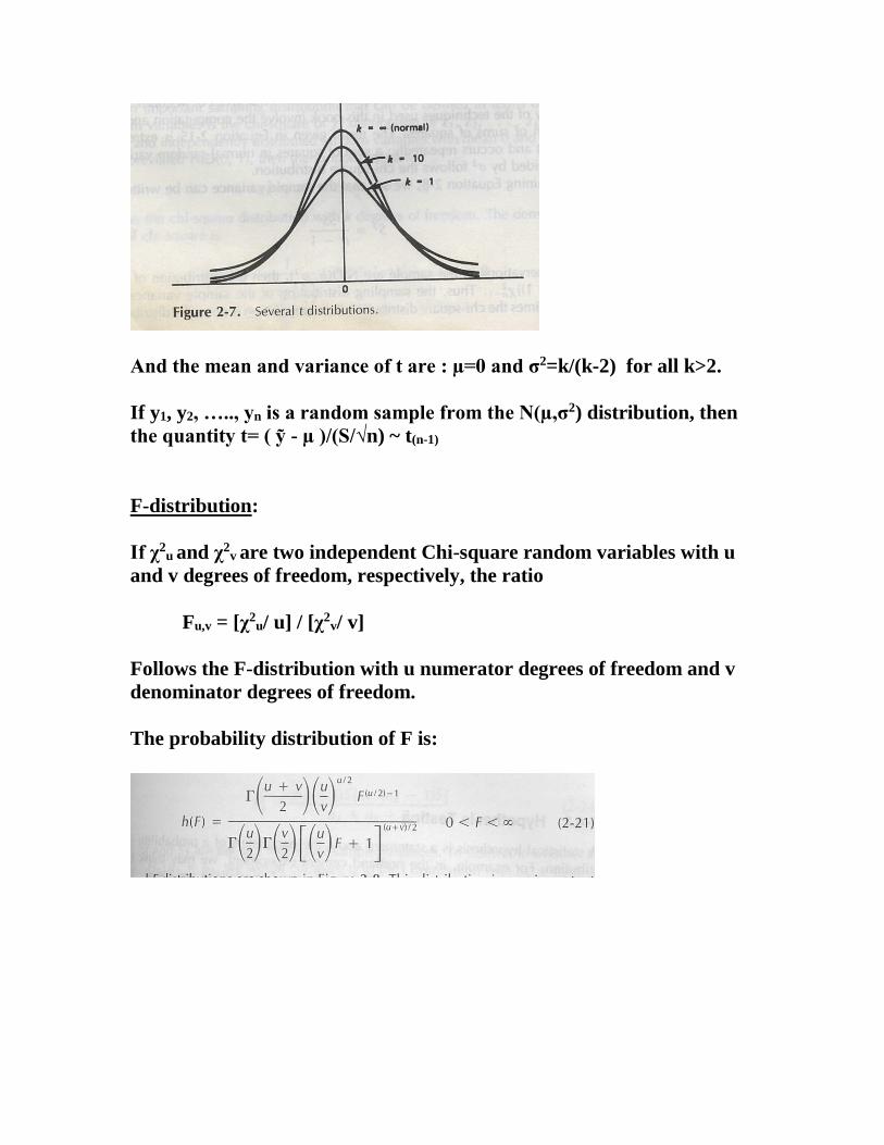
And the mean and variance of t are : µ=0 and σ2=k/(k-2) for all k>2.

If y1, y2, ….., yn is a random sample from the N(µ,σ2) distribution, then

the quantity t= ( ỹ - µ )/(S/√n) ~ t(n-1)

F-distribution:

If χ2u and χ2

v are two independent Chi-square random variables with u

and v degrees of freedom, respectively, the ratio

Fu,v = [χ2u/ u] / [χ2

v/ v]

Follows the F-distribution with u numerator degrees of freedom and v

denominator degrees of freedom.

The probability distribution of F is:

Example:

Suppose we have two independent normal populations with common

variance σ2. If y1,1, y1,2, ….., y1,n1 is a random sample of n1 observations

from the first population, and if y2,1, y2,2, ….., y2,n2 is a random sample of

n2 observations from the second, then

(S21/S2

2) ~ F(n1-1), (n2-1)

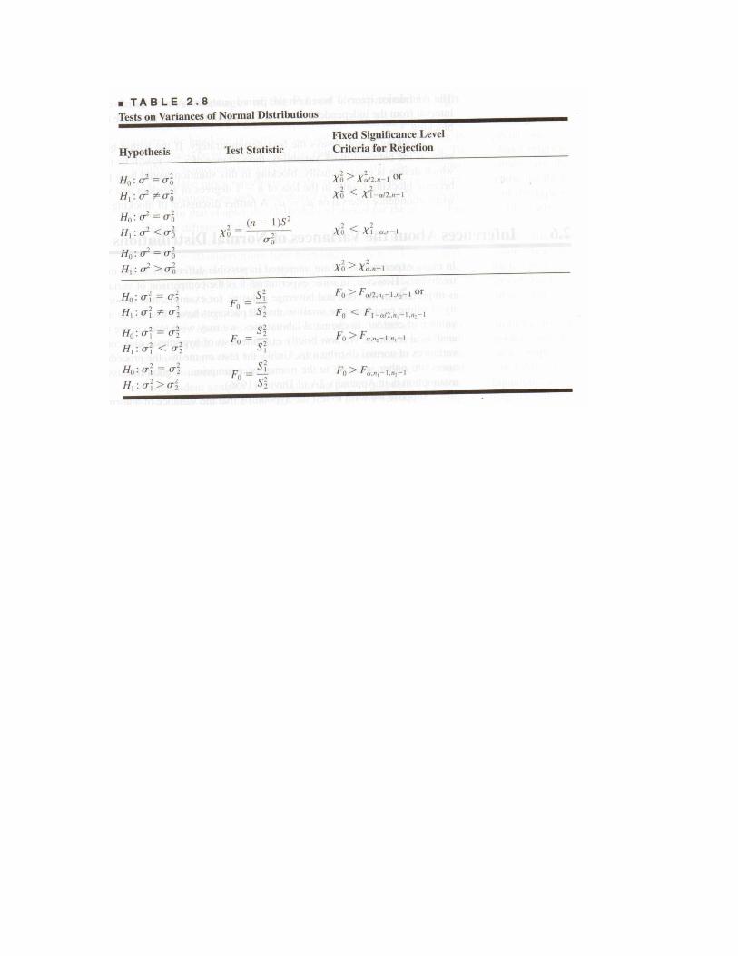
Inferences About Differences in Means, Randomized Designs:

Assumptions:

1- A completely randomized design is used.

2- The data are viewed as if they were a sample from a Normal

distribution.

Hypothesis testing:

A statistical hypothesis is a statement about the parameters of a

probability distribution.

Example: The Portland cement experiment)

We may think that the mean tension bond strengths of the two mortar

formulations are equal.

Ho: µ1= µ2

H1: µ1≠ µ2

The alternative hypothesis specified here is called a “two sided

alternative hypothesis” since it would be true either if µ1<µ2 or if µ1>µ2.

To test a hypothesis:

1- Take a random sample.

2- Compute an appropriate test statistic.

3- Reject or failing to reject Ho.

When testing hypothesis, two kinds of errors may be committed:

Type I Error: α = P(Type I Error)= P(Reject Ho│Ho: True)

Type II Error: β = P(Type II Error)= P(Failed to Reject Ho│Ho: False)

Power of the Test = (1- β) = P(Reject Ho│Ho: False)

The general Procedures in Hypothesis Testing:

1- Specify a value for α.

2- Design the test procedures so that β has a suitable small value.

Suppose that we could assume the variances of tension bond strengths

were identical for both mortar formulations. Then a test statistic

to=( ỹ1- ỹ2)/ Sp √[(1/n1) + (1/n2)]

Where;

Sp2=[(n1-1)S1

2 + (n2-1)S22]/(n1+n2-2)

Then, Reject Ho if │to│> t α /2, n1+n2-2

In some problems, one wish to reject Ho only if one mean is larger than

the other. Thus, one would specify a one-sided alternative hypothesis

H1: µ1>µ2 and would reject Ho if to > t α, n1+n2-2.

If one wants to reject Ho only if µ1 is less than µ2, then the alternative

hypothesis H1: µ1<µ2, and one would reject Ho if to < -t α, n1+n2-2.

Example:

Modified Mortar: ỹ1 = 16.76 kgf/cm2, S12= 0.316, n1=10

Unmodified Mortar: ỹ2 = 17.92 kgf/cm2, S22= 0.061, n2=10

Sp2 = [(n1-1) S1

2 + (n2-1)S22]/(n1+n2-2) = 0.081

Thus: Sp =0.284 and to = (ỹ1- ỹ2) / Sp √ [(1/n1) + (1/n2)]=-9.13

Therefore, reject Ho since │to│> t α /2, n1+n2-2= t 0.25,18 = 2.101.

Choice of Sample Size:

The choice of sample size and the probability of type II error β are

closely connected. Suppose that we are testing the hypothesis

Ho: µ1= µ2

H1: µ1≠ µ2

And the means are not equal so that ∂ = µ1- µ2.

Since Ho is not true, we are concerned about wrongly failing to reject

Ho. The probability of type II error depends on the true difference in

means ∂.

A graph of β versus ∂ for a particular sample size is called the operating

characteristic curve (or O. C. curve) for the test.

If β error is also a function of sample size, generally, for a given value of

∂, the β error decreases as the sample size increases.