ieee transactions on systems, man, and...

IEEE TRANSACTIONS ON SYSTEMS, MAN, AND CYBERNETICSŁPART B: CYBERNETICS 1

Exemplar-Based Human Action Pose CorrectionWei Shen, Ke Deng, Xiang Bai, Tommer Leyvand, Baining Guo, Fellow, IEEE, and Zhuowen Tu Member, IEEE,

Abstract—The launch of Xbox Kinect has built a very suc-cessful computer vision product and made a big impact tothe gaming industry; this sheds lights onto a wide variety ofpotential applications related to action recognition. The accurateestimation of human poses from the depth image is universallya critical step. However, existing pose estimation systems exhibitfailures when faced severe occlusion. In this paper, we propose anexemplar-based method to learn to correct the initially estimatedposes. We learn an inhomogeneous systematic bias by leveragingthe exemplar information within specific human action domain.Furthermore, as an extension, we learn a conditional model byincorporation of pose tags to further increase the accuracy ofpose correction. In the experiments, significant improvementson both joint-based skeleton correction and tag prediction areobserved over the contemporary approaches, including what isdelivered by the current Kinect system. Our experiments forfacial landmark correction also illustrate that our algorithm isapplicable to improve the accuracy of other detection/estimationsystems.

Index Terms—Kinect, random forest, pose correction, skeleton,pose tag.

I. INTRODUCTION

W ITH the development of high-speed depth cameras [1],the computer vision field has experienced a new op-

portunity of applying a practical imaging modality for buildinga variety of systems in gaming, human computer interaction,surveillance, and visualization. A depth camera provides depthinformation as different means to color images captured bythe traditional optical cameras. Depth information gives extrarobustness to color as it is invariant to lighting and texturechanges [2], although it might not carry very detailed infor-mation of the scene.

The human pose estimation/recognition component is akey step in an overall human action understanding system.High speed depth camera with the reliable estimation of thehuman skeleton joints [3] has recently led to a new consumerelectronic product, the Microsoft Xbox Kinect [1].

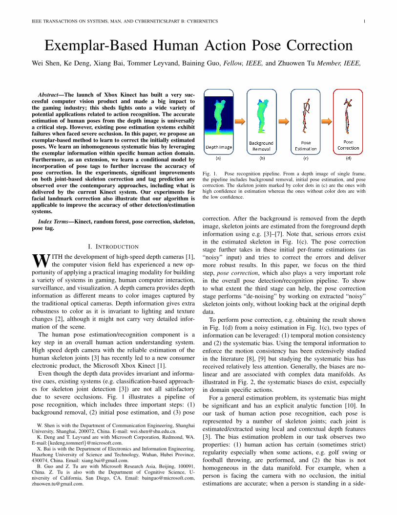
Even though the depth data provides invariant and informa-tive cues, existing systems (e.g. classification-based approach-es for skeleton joint detection [3]) are not all satisfactorydue to severe occlusions. Fig. 1 illustrates a pipeline ofpose recognition, which includes three important steps: (1)background removal, (2) initial pose estimation, and (3) pose

W. Shen is with the Department of Communication Engineering, ShanghaiUniversity, Shanghai, 200072, China. E-mail: [email protected].

K. Deng and T. Leyvand are with Microsoft Corporation, Redmond, WA.E-mail:{kedeng,tommerl}@microsoft.com.

X. Bai is with the Department of Electronics and Information Engineering,Huazhong University of Science and Technology, Wuhan, Hubei Province,430074, China. Email: [email protected].

B. Guo and Z. Tu are with Microsoft Research Asia, Beijing, 100091,China. Z. Tu is also with the Department of Cognitive Science, U-niversity of California, San Diego, CA. Email: [email protected],[email protected].

Fig. 1. Pose recognition pipeline. From a depth image of single frame,the pipeline includes background removal, initial pose estimation, and posecorrection. The skeleton joints marked by color dots in (c) are the ones withhigh confidence in estimation whereas the ones without color dots are withthe low confidence.

correction. After the background is removed from the depthimage, skeleton joints are estimated from the foreground depthinformation using e.g. [3]–[7]. Note that, serious errors existin the estimated skeleton in Fig. 1(c). The pose correctionstage further takes in these initial per-frame estimations (as“noisy” input) and tries to correct the errors and delivermore robust results. In this paper, we focus on the thirdstep, pose correction, which also plays a very important rolein the overall pose detection/recognition pipeline. To showto what extent the third stage can help, the pose correctionstage performs “de-noising” by working on extracted “noisy”skeleton joints only, without looking back at the original depthdata.

To perform pose correction, e.g. obtaining the result shownin Fig. 1(d) from a noisy estimation in Fig. 1(c), two types ofinformation can be leveraged: (1) temporal motion consistencyand (2) the systematic bias. Using the temporal information toenforce the motion consistency has been extensively studiedin the literature [8], [9] but studying the systematic bias hasreceived relatively less attention. Generally, the biases are no-linear and are associated with complex data manifolds. Asillustrated in Fig. 2, the systematic biases do exist, especiallyin domain specific actions.

For a general estimation problem, its systematic bias mightbe significant and has an explicit analytic function [10]. Inour task of human action pose recognition, each pose isrepresented by a number of skeleton joints; each joint isestimated/extracted using local and contextual depth features[3]. The bias estimation problem in our task observes twoproperties: (1) human action has certain (sometimes strict)regularity especially when some actions, e.g. golf swing orfootball throwing, are performed, and (2) the bias is nothomogeneous in the data manifold. For example, when aperson is facing the camera with no occlusion, the initialestimations are accurate; when a person is standing in a side-


view with certain hand motion, there is severe occlusion andthe initial estimation may not be all correct, as illustrated inFig. 1. In this paper, the main contribution is learning theinhomogeneous bias function to perform pose correction forone domain specific action and we emphasize the followingfour points: (1) exemplar-based approach serves a promisingdirection for pose correction in depth images, (2) learning aninhomogeneous regression function should naturally perfor-m data-partition, abstraction, and robust estimation. With athorough experimental study, our approach shows encouragingresults, (3) learning an regression function conditioned on aincorporated global parameter gives more nature data partition,thus further improve the performance of pose correction, (4)our regression based approach is general, it’s applicable tocorrecting not only the pose estimated from Kinect sensor,but also estimation errors involved from other sensors.

The remainder of this paper is organized as follows: Sec. IIreviews the works related to human pose estimation andcorrection. Sec. introduces the skeleton data and ground truthused in our work. Sec. IV describes the proposed approachto pose correction in detail. The experimental results onjoint-based skeleton correction, pose tag prediction and faciallandmark correction are presented in Sec. V. Finally, Sec. VIdraws conclusions and points out potential directions for futureresearch.

This paper extends our preliminary work [11] with thefollowing contributions: (1) the proposal of a conditionalregression model as well as the cascaded one, which furtherenhance the pose correction performance, (2) tag predictionexperiments on a new football throwing data set, (3) landmarkcorrection experiments to show the generality of the proposedmethod.

Fig. 2. Three groups of poses. In each group, the poses are similar, andthe errors of the estimated skeletons are somewhat systematic, e.g. the rightforearms of the skeletons in the second group and those in the third group.

II. RELATED WORK

Motion and action recognition from optical cameras hasbeen an active research area in computer vision; typical ap-proaches include 3D feature-based [12], part-based (poselets)[13], and segment-based [14] approaches. Although insights

can be gained, these methods are not directly applicable toour problem.

Benefit from rapid development of the real-time depthcamera, action recognition from depth images has been a hottopic in recent years. Shotton et al. [3] cast pose estimationas a per-pixel classification problem. They compute the depthcomparison feature [15] of each pixel, then classify each pixelinto human parts. Finally the modes of probability mass foreach part are take as the joint position proposals. Girshicket al. [4] improve Shotton’s method, they predict the offsetbetween each pixel and each joint by regression instead. Sunet al. [5] follows Girshick’s regression-based method, they leanthe regression model conditioned on several global parameters,such as height and torso orientation. Ye et al. [6] proposeto search the most similar pose in the database by matchingthe cloud points of the depth images and then refine the bestmatching pose to be the estimated pose. Baak et al. [7] alsopropose a data driven approach for pose estimation, insteadof matching cloud points, they extract features from the depthdata and then measure the similarity between the extractedfeatures. A recent survey on the human action analysis withKinect depth sensor can be found in [16]. These methodsprovide the direct input for our method, so our methodwill benefit from the improvement of these pose estimationmethods.

From a different view, bias estimation has been a longstanding problem in statistics [10]. Related work in the posecorrection task uses physical-model-based approaches [17],Kalman-like filters [18], or exemplar-based approaches butwith very specific design, which is hard to adapt to the generaltask [19]. Here we adopt the random forest regressor, whichtakes in both the estimated solutions and their estimationuncertainties. We show significant improvement over other re-gressors such as nearest neighborhood [20], Gaussian processregression [21], support vector regression [22], and logisticregression [23]. Our approach is real-time and can be directlyapplied to the Kinect system.

III. DATA

In this section, we introduce the data used for our posecorrection problem. The recently launched Kinect camera [1]is able to give 640× 480 image at 30 frames per second withdepth resolution of a few centimeters. Employing the Kinectcamera, we are able to generate a large number of realisticdepth images of human poses. The human skeleton estimatedfrom the depth image by the current Kinect system [3] is thedirect input for our approach, which is called ST (SkeletonesTimation) in the rest of this paper. As shown in Fig. 3(a),there are 20 body joints in a skeleton, including hips, spine,shoulders, head, elbows, wrists, hands, knees, ankles, and feet.

As suggested by the recent work [3], [4], the ground truthpositions of the body joints can be captured by motion capture(mocap) system. We obtain a set of mocap of human actionsas the ground truth of the estimated skeletal joints. The mocapdata is also called GT (Ground Truth) in the rest of this paper.In our experiments, we limit the rotation of the user to ±120◦

in both training and testing data. Fig. 3(b) shows several pairsof ST and GT.


Fig. 3. Skeleton data. (a) A template skeleton and its joints. The skeleton is a simple directed graph, in which the directions are denoted by the arrowsbeside the skeleton edges. For denotational simplicity, we do not show the arrows in other figures. (b) Several pairs of input noisy skeletons (upper) andground truth skeletons (lower).

Fig. 4. Pose tag. Each type of poses are assigned to a tag, e.g. the tag of“front swing” (the last pose) is about 0.95.

As for gaming applications, skeletons with 20 joints are toomuch data for games to process, since they usually only needone or two global parameters to describe the motion. So posetag is introduced to be used to drive the avatar to put on thesame pose as the player performs in the somatosensory game.The pose tag is a real value ranging from 0.0 to 1.0, indicatinga specific stage in a particular action, e.g. golf swing. In adomain of specific action, each type of poses is assigned a tagmanually. For example, the tag value of the poses of ”frontswing” and ”back swing” are within the intervals [0.8 1.0] and[0.0 0.2] respectively. The accurate value is determined by theamplitude of swing. Fig. 4 shows the tag values of a typicalgolf swing action. We will demonstrate how to enhance posecorrection by incorporating pose tags.

IV. POSE CORRECTION

A. Objectives

We focus on two tasks: joint-based skeleton correction andpose tag prediction. Our inputs are m estimated skeletonsst = (ST1, . . . , STm) from a video sequence of m depth im-age frames. Each skeleton estimation ST includes n (n = 20here) joints: ST = (xj , cj ; j = 1, . . . , n), where xj ∈ R3

denotes the world coordinates of the jth body joint, as shownin Fig. 3. cj indicates the confidence for the estimation xj bythe skeleton joint detector, i.e. if joint j has high confidence,cj = 1; Otherwise, cj = 0. For example, in Fig. 1(c), the

skeleton joints marked by color dots are the ones with highconfidence in estimation whereas the ones without color dotsare with the low confidence.

The first task (joint-based skeleton correction) is to predictthe “true” position of each joint: xj → xj and the “true”skeletons gt = (GT1, . . . , GTm) where each GT = (xj ; j =1, . . . , n) and xj ∈ R3. In training, we are given a trainingset of {(st,gt)k}Kk=1 of K pairs of st and gt; in testing, wewant to predict the “true” gt from a given input st.

The second task (pose tagging) is to predict the pose tagΥ = (Υ1, . . . ,Υm) from a given st = (ST1, . . . , STm). Intraining, we are given a training set of {(st,Υ)k}Kk=1 of Kpairs of st and Υ; in testing, we want to predict the tag valuesΥ from a given input st.

The tag is actually a low dimensional manifold coordinateof the pose. As for gaming applications, tag predication isimportant for games even when perfect skeletons are available.Both of the two tasks are performed to recover the pose froma noisy initial estimation, so we categorize them into the tasksof pose correction.

B. Normalized Skeleton Joints Coordinates

From the world coordinates, we want to have an intrinsicand robust representation. Based on the n = 20 joints,we show the kinematic skeleton template as displayed inFig. 3(a), which is a directed graph. Each joint is a nodeof the graph. Given an ST = (xj , cj ; j = 1, . . . , n), wecompute its normalized coordinates for our problem, denotedas H(ST ) = (rj , cj ; j = 1, . . . , n). Since xj denotes theworld coordinate, we normalize them to the template toremove not only the global translation but also the variation inindividual body differences. We use the skeleton joint C. Hipas the reference point, the origin, r1 = (0, 0, 0), and map theother joints to the sphere as rj =

xj−xjo

∥xj−xjo∥2where joint jo

is the direct predecessor of joint j on the skeleton (directedgraph).

The design of the transformed coordinates H(ST ) is moti-vated by the kinematic body joint motion. H(ST ) observes acertain level of invariance to translation, scaling, and individ-ual body changes. We can actually drop r1 since it is alwayson the origin. One could add other features computed on ST


to H(ST ) to make it more informative but this could be atopic of future research.

C. Joint-based Skeleton Correction

1) Joint offset inference: To perform skeleton correctionfrom a noisy input ST , instead of directly predicting the “true”positions of the body joints, we infer the offsets between thejoints in the ST and those in the GT . This has its immediatesignificance: when a person is facing the camera with noocclusion, ST is actually quite accurate, and thus has nearlyzero difference to GT ; when a person is playing the gamein side view with severe occlusions, there is often a largeand inhomogeneous difference between ST and GT . This isessentially a manifold learning problem. Certain clusters ofST on the manifold can directly be mapped to, e.g. very lowvalues, if we would predict the offsets; predicting the directcoordinates of GT however would have to explore all possibleST in the data space.

Now we show how to compute the offsets between the jointsin ST = (xj , cj ; j = 1, . . . , n) and those in GT = (xj ; j =1, . . . , n), where xj ,xj ∈ R3 are the world coordinates ofjoint j in ST and GT , respectively. To ensure the scaleinvariance of the offsets, skeletons are normalized based on thedefault lengths of the skeleton edges in the template shown inFig. 3(a). First, we choose a set of stable joints JS = {Spine,C. Shoulder, Head, L. Hip, R. Hip, L. Knee, R. Knee, L. Ankle,R. Ankle }. We call them stable joints because other joints inthe ST , such as Hand and Wrist, are often occluded by thehuman body, thus the skeleton edge lengths between themare prone to errors. Given an ST , for each skeleton edgebetween the stable joints and their direct predecessors, wecompute the proportion to the template skeleton edge length:λ(j, jo) = ∥xj − xjo∥2/∥Tj − Tjo∥2, where Tj is the jthjoint for the template T (shown in Fig. 3), which is fixedin this problem. Suppose that there is no error in the ST , thenfor each j ∈ JS , λ(j, jo) is nearly identical. However, theestimation error may result in a serious bias when computingλ(j, jo). Although we only consider the stable joints, theirestimated positions may also be wrong. Therefore, we shouldexclude the joints with large estimation error, and averagethe skeleton edge lengths between the rest joints to obtaina robust measure of the scale of the ST . To this end, the scaleproportion of the ST is formulated by

λ(ST ) =

∑j∈JS

λ(j, jo) · δ(∥λ(j, jo)−∑

λ(j,jo)|JS | ∥1 ≤ th)∑

j∈JSδ(∥λ(j, jo)−

∑λ(j,jo)|JS | ∥1 ≤ th)

,

(1)where δ(·) is an indicator function which is a robust measureto exclude the outliers and

th = 3

√√√√∑j∈JS

(λ(j, jo)−∑

λ(j,jo)|JS | )2

|JS |. (2)

Here we define the threshold th as the triple standard deviationto exclude the outliers according to the 3-sigma rule. Finally,the offset of a joint j between the pair of xj and xj iscomputed as

∆j = (xj − xj)/λ(ST ), (3)

and D = (∆1, . . . ,∆n) for each skeleton of n joints. For theentire sequence of m images, we have d = (D1, . . . ,Dm).Note that we do not need to explicitly align the pair of STand GT , since they are obtained from the same depth image.

2) Learning the regression for joint offsets : In this section,we discuss how to learn a regression function to predict theoffset to perform pose correction. We are given a training set ofS = {(st,gt)k}Kk=1 of K pairs of st and gt (for denotationalsimplicity, we let K = 1 and thus k can be dropped for aneasier problem understanding). Using the normalization stepin Sec. IV-B, we obtain h(st) = (H(ST1), . . . ,H(STm))where each H(ST ) = (rj , cj ; j = 1, . . . , n); using theoffset computing stage in Eq. 3, we compute the offset,d = (D1, . . . ,Dm). Thus, our goal is to predict the mappingh(st) → d.

We first learn a function to directly predict the mappingfd : H(ST ) → D by making the independent assumptionof each pose. From this view, we rewrite the training set asS = {(H(STi),Di)}mi=1.

Random forest [24]–[26] includes an ensemble of tree pre-dictors that naturally perform data-partition, abstraction, androbust estimation. For the task of regression, tree predictorstake on target values and the forest votes for the most possiblevalue. Each tree in the forest consists of split nodes andleaf nodes. Each split node stores a feature index with acorresponding threshold τ to decide whether to branch tothe left or right sub-tree and each leaf node stores somepredictions. Each leaf node stores a set of exemplars in apartitioned feature subspace with similar target values. Theprediction of the tree is the abstraction of the target values ofthe exemplars within one leaf node. Therefore, it’s proper toapply random forest regression to predict the inhomogeneoussystematics bias.

Our objective is to learn a random forest regression func-tion fd : H(ST ) → D. Following the standard greedydecision tree training algorithm [3], [4], [15], each tree inthe forest is learned by recursively partitioning the train-ing set S = {(H(STi),Di)}mi=1 into left Sl and rightSr subsets according to the best splitting strategy θ∗ =argminθ

∑p∈{l,r}

|Sp(θ)||S| e(Sp(θ)), where e(·) is an error

function standing for the uncertainty of the set and θ is aset of splitting candidates. If the number of training samplescorresponding to the node (node size) is larger than a maximalκ, and

∑p∈{l,r}

|Sp(θ∗)|

|S| e(Sp(θ∗)) < e(S) is satisfied, then

recurse for the left and right subsets Sl(θ∗) and Sr(θ

∗),respectively.

The selection of the error function e(·) is important forlearning an effective regressor. Here, we employ the rootedmean squared differences:

e(S) =

√∑mi=1 ∥Di −

∑mi=1 Di

|S| ∥22m

. (4)

In the training stage, once a tree t is learned, a set of trainingsamples Slf

t = {Dlfi }|S

lft |

i=1 would fall into a particular leafnode lf . Obviously, it is not effective to store all the samples inSlft for each leaf node lf . Instead, we would do an abstraction

for the learning purpose. One choice is to store the mean


D(lf) =∑

i Dlfi /|Slf

t | of the set Slft . One could store other

abstractions such as the histogram of Slft as well. In addition,

each tree t would assign a leaf node label Lt(H(STi)) for agiven H(STi).

In the testing stage, given a test example ST = (xj , cj ; j =1, . . . , n), for each tree t, it starts at the root, then recur-sively branches left or right. Finally, it reaches the leaf nodeLt(H(ST )) in tree t, then the prediction given by tree t isFt(H(ST )) = δ(lf = Lt(H(ST ))) · D(lf), where δ(·) is anindicator function. The final output of the forest (T trees) isa probability function:

PH(ST )(D) =1

T

T∑t=1

exp(−∥D− Ft(H(ST ))

hD∥22), (5)

where hD is a learned bandwidth. The mean can be con-sidered as another output of the learned regression functionfd(H(ST )) = EPH(ST )

[D] where EPH(ST )[·] indicates the

expectation. The corrected skeleton is obtained by (if wewould use the fd(H(ST )) as the output)

CT = ST− + λ(ST ) · fd(H(ST )), (6)

where ST− = (xj ; j = 1, . . . , n) and the components in CTare CT = (zj ; j = 1, . . . , n). In the experiments, we refer tothis method (using the fd(H(ST )) as the output) as RFR.

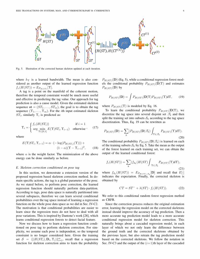
3) Regression cascade: In the recent work [27], an algo-rithm named cascaded pose regression (CPR) is proposed,which iteratively trains a series of regressors to approachthe ground truth. Inspired by CPR, we propose a regressioncascade (RFRC) here.

As described in Sec. IV-C2, we learn a regression functionfd : H(ST ) → D. Here, we rewrite it as

f(0)d : H(ST ) → D(0). (7)

Then we obtain the corrected skeleton CT (1) by

CT (1) = ST− + λ(ST ) · f (0)d (H(ST )). (8)

Then we compute the normalized skeleton joint coordinatesH(CT (1)) and learn the second layer of regression function:

f(1)d : (H(ST ),H(CT (1))) → D(1), (9)

where D(1) is the offsets between CT (1) and GT computed bythe stage in Eq. 3. Then repeat the process mentioned above.The (i+ 1)th layer of regression function is

f(i)d : (H(ST ),H(CT (i))) → D(i). (10)

The output skeleton is

CT (i+1) = CT (i) + λ(ST ) · f (i)d (H(ST ),H(CT (i))). (11)

For consistency, we define CT (0) = ∅ and obtain

CT (i+1) = ST− + λ(ST ) ·i∑

ι=0

f(ι)d (H(ST ),H(CT (ι))).

(12)Fig. 5 shows an illustration for the process of the regression

cascade.

4) Temporal constraint: Taking the motion consistency intoaccount, we could use the temporal constraint to improve ourcorrection results. Our learned regression function outputs aprobability distribution as shown in Eq. (5), which can beused to employ the temporal information. Given the estimatedskeleton sequence st = (ST1, . . . , STm), our goal is to obtainh(st) → d, where d = (D1, . . . ,Dm), with the correspond-ing corrected skeleton sequence ct = (CT1, . . . , CTm). Tomeet the real time requirement, our approach follows a causalmodel, i.e. the current prediction only depends on past/currentinputs/outputs. For the ith input estimated skeleton STi, itsoffset is computed as

Di =

{fd(H(STi)) if i = 1

arg minD∈Rn×3

E(D|STi, STi−1,Di−1) otherwise ,

(13)where E(·) is an energy function defined as

E(D|STi, STi−1,Di−1) = α · (− log(PH(STi)(D))) +

(1− α)∥ST−i + λ(STi)D− (ST−

i−1 + λ(STi−1)Di−1)∥22, (14)

where α is a weight factor. We use coordinate descent to solveEq. 14. Finally, the corrected skeleton CTi is

CTi = ST−i + λ(STi)Di. (15)

In the experiments, we refer to the random forest regressionand cascade methods under temporal constraint as RFRT andRFRCT respectively. In the cascaded method, the temporalconstraint is only used in the regressor of the last layer andthe regressors of the former layers use the expectation as theoutput.

D. Pose tag prediction

In this section we discuss how to learn a regression func-tion to predict the tag of a pose. The learning process isthe same as what we did for the skeleton correction; sowe follow the notions in Sec. IV-C2 and IV-C4 except forreplacing the offset D by the tag value Υ. As stated in theprevious section: we are given a training set {(st,Υ)k}Kk=1

of K pairs of st and Υ (for denotational simplicity, welet K = 1 and thus k can be dropped for easier problemunderstanding). Using the normalization step in Sec. IV-B,we obtain h(st) = (H(ST1), . . . , H(STm)), where eachH(ST ) = (rj , cj ; j = 1, . . . , n). Thus our objective is toobtain h(st) → Υ, where st = (STi; i = 1, . . . ,m) and(Υ = Υi; i = 1, . . . ,m). Similarly, a random forest regressionfunction to directly predict the tag only based on the individualskeleton fυ : H(ST ) → Υ is also learned first. Here, each leafnode in tree t also stores the mean tag values of the samplesfalling into the leaf node. In the testing stage, given a testexample ST , the prediction Ft(H(ST )) given by tree t isalso computed similarly as in Sec. IV-C2. The final output ofthe forest (T trees) is a regression in probability function:

PH(ST )(Υ) =1

T

T∑t=1

exp(−∥Υ− Ft(H(ST ))

hΥ∥2), (16)


Fig. 5. Illustration of the corrected human skeleton updated at each iteration.

where hΥ is a learned bandwidth. The mean is also con-sidered as another output of the learned regression functionfυ(H(ST )) = EPH(ST )

[Υ].A tag is a point on the manifold of the coherent motion,

therefore the temporal constraint would be much more usefuland effective in predicting the tag value. Our approach for tagprediction is also a cause model. Given the estimated skeletonsequence st = (ST1, . . . , STm), the goal is to obtain the tagsequence (Υ1, . . . ,Υm). For the ith input estimated skeletonSTi, similarly Υi is predicted as:

Υi =

{fυ(H(STi)) if i = 1

arg minΥ∈[0,1]

E(Υ|STi,Υi−1) otherwise , (17)

where

E(Υ|STi,Υi−1) = α · (− log(PH(STi)(Υ))) +

(1− α)(Υ−Υi−1)2, (18)

where α is the weight factor. The minimization of the aboveenergy can be done similarly as before.

E. Skeleton correction conditioned on pose tag

In this section, we demostrate a extension version of theproposed regression based skeleton correction method. In do-main specific actions, the tag is a global parameter of the pose.As we stated before, to perform pose correction, the learnedregression function should naturally perform data-partition.According to tags, pose data space is naturally partitioned intoseveral subspaces, therefore we can learn several conditionalprobabilities over the tag space instead of learning a regressionfunction on the whole pose data space as we did in Sec. IV-C2.The motivation is that conditional probabilities are easier tolearn since the regression trees do not have to deal with allpose variations. This is inspired by Dantone’s work [28], whichlearns conditional regression forests to detect facial feature.

Now we discuss how to learn a regression function condi-tioned on pose tag to perform skeleton correction. For sim-plicity, we assume each pose is independent, so the temporalconstraint is no longer considered here. Given the trainingset S = {(H(STi),Di,Υi)}mi=1, recall that a regressionfunction for skeleton correction aims to learn the probability

PH(ST )(D) (Eq. 5), while a conditional regression forest mod-els the conditional probability PH(ST )(D|Υ) and estimatesPH(ST )(D) by

PH(ST )(D) =

∫PH(ST )(D|Υ)PH(ST )(Υ)dΥ, (19)

where PH(ST )(Υ) is modeled by Eq. 16.To learn the conditional probability PH(ST )(D|Υ), we

discretize the tag space into several disjoint set Tk and thensplit the training set into subsets Sk according to the tag spacediscretization. Thus, Eq. 19 can be rewritten as

PH(ST )(D) =∑k

(PH(ST )(D|Tk)

∫Υ∈Tk

PH(ST )(Υ)dΥ).

(20)The conditional probability PH(ST )(D|Tk) is learned on eachof the training subsets Sk by Eq. 5. Take the mean as the outputof the forest learned on each training set, we can obtain theoutput of the learned conditional forest:

fc(H(ST )) =∑k

(fdk(H(ST )

∫Υ∈Tk

PH(ST )(Υ)dΥ),

(21)where fdk

(H(ST )) = EPH(ST ),Tk[D] and recall that E[·]

indicates the expectation. Finally, the corrected skeleton isobtained by

CT = ST− + λ(ST ) · fc(H(ST )). (22)

We refer to this conditional random forest regression methodas CRFR.

Since the correction process reduces the original estimationerror, learning the regression model on the corrected skeletonsinstead should improve the accuracy of tag prediction. Then amore accurate tag prediction model leads to a more accurateconditional regression model for skeleton correction. Thisnaturally brings about a cascaded regression model, in eachlayer of which we not only learn the difference betweenthe ground truth and the corrected skeletons obtained bythe previous layer, but also retrain the tag prediction modelbased on the corrected skeletons. We follow the notation inSec. IV-C3 and the output of the (i+1)th layer of the cascaded


model is obtained by

CT (i+1) = ST− + λ(ST ) ·i∑

ι=0

f (ι)c (H(ST ),H(CT (ι))),

(23)where

f (ι)c (H(ST ),H(CT (ι)))) =

∑k

(f(ι)dk

(H(ST ),H(CT (ι)))∫Υ∈Tk

PH(ST ),H(CT (ι))(Υ)dΥ), (24)

Similar as we trained skeleton correction model in Sec. IV-C3,here we concatenate normalized skeleton joint coordinates ofthe corrected skeletons H(CT (ι)) to H(ST ) to train the tagprediction model of each layer: PH(ST ),H(CT (ι))(Υ). We referto the proposed cascaded conditional random forest regressionmethod as CRFRC.

V. EXPERIMENTAL RESULTS

In this section, we show the experimental results and givethe comparisons between alternative approaches, includingwhat is delivered in the current Kinect system. In the re-mainder of this section, unless otherwise specified, we setthe parameters for learning random forest as: the number oftrees T = 50 and leaf node size κ = 5. The bandwidths hD

and hΥ and the weight factor α are optimized on a hold-outvalidation set by grid search (As an indication, this resultedin hD = 0.01m, hΥ = 0.03 and α = 0.5). We set the numberof the layers of regression cascade as L = 2.

A. Joint-based skeleton correction

To evaluate our algorithm, we show the performance on achallenging data set. This data set contains a large numberof poses, 15, 815 frames in total, coming from 81 golf swingmotion sequences. Some pose examples are shown in Fig. 3.We select 19 sequences containing 3, 720 frames as thetraining data set. The rest 12, 095 frames are used for testing.

1) Error Metrics: Given a testing data set {(STi, GTi)}mi=1,we obtain the corrected skeletons {CTi; i = 1, . . . ,m}. Wemeasure the accuracy of each corrected skeleton CT =(zj ; j = 1, . . . , n) by the sum of joint errors (sJE) GT =(xj ; j = 1, . . . , n): ε =

∑j ∥zj − xj∥2. To quantify the

average accuracy on the whole testing data, we report the meansJE (msJE) across all testing skeletons:

∑i εi/m (unit: meter).

2) Comparisons: In this section, we give the comparisonbetween the methods for joint-based skeleton correction.Current Kinect approach. To illustrate the difficulty of theproblem, we compare with the approach in the current Kinectsystem. The current Kinect system for skeleton correction iscomplex, which employs several strategies such as temporalconstraint and filtration. The main idea of the approach isnearest neighbor search. For a testing ST , The approachsearches its nearest neighbor in the estimated skeletons in thetraining set. Then the ground truth of the nearest neighboris scaled with respect to ST to be the corrected skeleton ofST . The details of this system is unpublished. We refer tothe current approach in Kinect system as K-SYS in the rest of

Fig. 6. Comparison with several methods on our testing data set. Thequantitative results are illustrated in the left-hand bar graph and the accuratevalues are listed in the right-hand table. The baseline is the msJE of the inputtesting estimated skeletons.

paper. On the whole testing set, K-SYS achieves 2.0716 msJE,while RFR achieves 1.5866. We illustrate some examples ofthe corrected skeletons obtained by K-SYS and our algorithmin Fig. 7. The skeletons obtained by our algorithm are moresimilar to the ground truths.Regress the absolute joint position. To show the significanceof learning the offsets between joints in ST and GT , wealso give the result by directly predicting the absolute jointposition by random forest regression (RFRA). To learn theabsolute position, for each GT = (xj ; j = 1, . . . , n) inthe training set S = {(STi, GTi)}mi=1, we translate theC. Hip x1 to (0, 0, 0) to align them. The absolute jointposition of each GT = (xj ; j = 1, . . . , n) is obtainedby xj = (xj − x1)/λ(GT ). Then a regression functionf : H(ST ) → (x1, . . . , xn) is learned as the process inSec. IV-C2. Given a testing ST = (xj ; j = 1, . . . , n), the jointpositions of the corrected skeleton CT = (zj ; j = 1, . . . , n)are obtained by CT = λ(ST )f(H(ST )). Finally, the C. Hipz1 of the obtained CT is translated to x1 to align the CTwith the ST . As shown in Fig. 6, RFRA does not perform aswell as RFR.Other regression algorithms.We also apply other regressionalgorithms to joint-based skeleton correction, such as Gaussianprocess regressor [21] (GPR) and support vector regressor [22](SVR). The implementation of GPR was taken from theGPML toolbox [29], which learns the parameters of the meanand covariance functions of Gaussian processes automatically.GPR achieves 1.7498 msJE. Fig. 6(a) shows the apparentadvantage of RFR over GPR. We employ the implementationof SVR taken from the package of LIBSVM [30]. We utilizeradial basis function (RBF) kernel for SVR and obtain 1.6084msJE. The result obtained by SVR is also worse than RFR.Besides, to train the model of SVR, quite a few parametersneed to be tuned.

We illustrate the performances of all the methods mentionedabove in Fig. 6. The baseline is the msJE of the input estimatedskeletons, which is 2.3039 msJE. RFRT, RFRC and RFRCTachieve 1.5831, 1.5766 and 1.5757, respectively. The resultsdemonstrate that both performing in the way of cascade andadding temporal constraint can help improve the performance.Different joints are under occlusions of different degrees,e.g. the head is rarely under occlusion and the elbows are


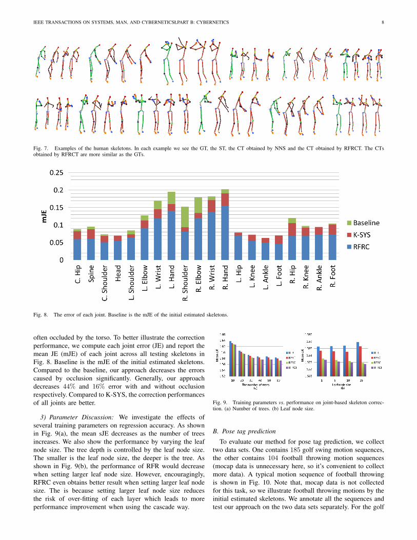
Fig. 7. Examples of the human skeletons. In each example we see the GT, the ST, the CT obtained by NNS and the CT obtained by RFRCT. The CTsobtained by RFRCT are more similar as the GTs.

Fig. 8. The error of each joint. Baseline is the mJE of the initial estimated skeletons.

often occluded by the torso. To better illustrate the correctionperformance, we compute each joint error (JE) and report themean JE (mJE) of each joint across all testing skeletons inFig. 8. Baseline is the mJE of the initial estimated skeletons.Compared to the baseline, our approach decreases the errorscaused by occlusion significantly. Generally, our approachdecreases 44% and 16% error with and without occlusionrespectively. Compared to K-SYS, the correction performancesof all joints are better.

3) Parameter Discussion: We investigate the effects ofseveral training parameters on regression accuracy. As shownin Fig. 9(a), the mean sJE decreases as the number of treesincreases. We also show the performance by varying the leafnode size. The tree depth is controlled by the leaf node size.The smaller is the leaf node size, the deeper is the tree. Asshown in Fig. 9(b), the performance of RFR would decreasewhen setting larger leaf node size. However, encouragingly,RFRC even obtains better result when setting larger leaf nodesize. The is because setting larger leaf node size reducesthe risk of over-fitting of each layer which leads to moreperformance improvement when using the cascade way.

Fig. 9. Training parameters vs. performance on joint-based skeleton correc-tion. (a) Number of trees. (b) Leaf node size.

B. Pose tag prediction

To evaluate our method for pose tag prediction, we collecttwo data sets. One contains 185 golf swing motion sequences,the other contains 104 football throwing motion sequences(mocap data is unnecessary here, so it’s convenient to collectmore data). A typical motion sequence of football throwingis shown in Fig. 10. Note that, mocap data is not collectedfor this task, so we illustrate football throwing motions by theinitial estimated skeletons. We annotate all the sequences andtest our approach on the two data sets separately. For the golf


Fig. 10. A typical motion sequence of football throwing.

Fig. 11. Comparison with several methods on the golf swing data set. (a)The quantitative results obtained by several methods. (b) Accuracy versus sizeof training data set.

Fig. 12. Comparison with several methods on the football throwing data set.(a) The quantitative results obtained by several methods. (b) Accuracy versussize of training data set.

swing data set, 37 sequences containing 3, 066 frames are usedfor training; the rest 148 sequences containing 12, 846 framesare used for testing. For the football throwing data set, 21sequences containing 1, 277 frames are used for training; therest 83 sequences containing 4, 108 frames are used for testing.In addition, we also did various folds of cross-validation to testthe stability of our approach.

1) Error Metrics: Given the testing data set{(STi,Υi)}mi=1, where Υi is the annotated tag of STi,we obtain the predicted tags {Υi}mi=1. The tag predictionaccuracy on the whole testing data set is quantified by the

rooted mean square (RMS) distance:√

Σmi=1(Υi −Υi)2/m.

2) Comparisons: In this section, we give the comparisonbetween the methods for tag prediction.Current Kinect approach. The current approach in Kinectsystem (K-SYS) for tag prediction also contains many detailssuch as imposing temporal constraint and filtering. The mainidea of K-SYS is also nearest neighbor search. For a testingST , K-SYS searchs its nearest neighbor in training set, thenthe predicted tag of its nearest neighbor is taken as the tag ofthe ST . On the football throwing data set, K-SYS achieves

0.1104 RMS, which is worse than RFR (0.0976 RMS). RFRTis the best, which achieves 0.0918 RMS. On the golf swingdata set, K-SYS achieves 0.1376 RMS, which is even betterthan RFR (0.1406 RMS). The reason may be the golf swingdata set is more challenging (there are much more occlusions),so the prediction from a single frame is more inaccurate. Inthis case, the temporal constraint plays a more important rolein tag prediction. Our algorithm RFRT significantly improvesRFR, it achieves 0.1164 RMS. We also compare with K-SYSby varying the size of training data set. We divide each dataset into 10 folds with equal sizes, then randomly select Nt

folds for training and use the rest for testing. We computethe mean and the standard deviation of the RMS distancesobtained by repeating the random selection for 5 times. Theresults for Nt = 4, 6, 8 using 10 trees on the golf swing dataset and the football throwing data set are shown in Fig. 11(b)and Fig. 12(b) respectively.K-nearest neighbors search. To show the advantage ofrandom forest in data abstraction and robust estimation,we compare with K-nearest neighbors search (KNNS). Giv-en a testing sequence (ST1, . . . , STm), for each STi(i ∈(1, . . . ,m)), K nearest neighbors are searched from thetraining set, and the tags of the neighbors are obtained:ΥK = (Υk; k = 1, . . . ,K). Then we obtain the probabilitydistribution PH(STi)(Υ) = 1

K

∑Kk=1 exp(−∥Υ−Υk)

hΥ∥2). Then

considering the temporal consistency, using the method inSec. IV-D, the optimal value is searched from the distributionPH(STi)(Υ) as the predicted tag of STi. KNNS only achieves0.1451 RMS and 0.1311 RMS on the golf swing data set andthe football throwing data set, respectively.Other regression algorithms. We apply GPR and SVR totag prediction, which achieve 0.1563 RMS and 0.1426 RMSon the golf swing data set respectively and achieve 0.1208RMS and 0.1174 RMS on the football throwing data setrespectively. The tag is a real value ranging from 0.0 to 1.0, sowe also apply logistic regression (LR) [23] to tag prediction.However, it only achieves 0.1806 RMS and 0.1322 RMS onour two data sets, respectively. Unlike RFR, which benefitsfrom optimization under the temporal constraint, GPR, SVRand LR have no such advantage.

We illustrate the results of tag prediction on our two datasets in Fig. 11(a) and Fig. 12(a), respectively. Fig. 13 andFig. 14 shows tag curves of four example sequences from thetwo data sets, respectively. The horizontal and vertical axes ofthe tag curve are the frame index of the sequence and the tagvalue, respectively. The curves obtained by RFRT (black) fitthe annotated curves (green) best.

3) Parameter Discussion: The effects of the training pa-rameters, including the number of trees and leaf node size, ontag prediction accuracy is shown in Fig. 15. Generally, usingmore trees and setting smaller leaf node size help improve theperformance.

C. Skeleton correction conditioned on pose tag

Not all the frames in the data set used in Sec. V-A areannotated with tag values, so we select the annotated framesfrom it which form a subset to evaluate the conditional random


Fig. 13. The tag curves of four example sequences from the golf swingdata set. In each example, we show the annotated curve (green) and thoseobtained by K-SYS (red), RFR (blue) and RFRT (black). The black curvesfit the green best.

Fig. 14. The tag curves of four example sequences from the football throwingdata set. In each example, we show the annotated curve (green) and thoseobtained by K-SYS (red), RFR (blue) and RFRT (black). The black curvesfit the green best.

Fig. 15. Training parameters vs. performance on tag prediction. (a) Numberof trees. (b) Leaf node size.

forest regression method. The subset contains 6, 452 frames intotal, from which 2, 352 are randomly selected as the trainingset and the rest are used as the testing set. To train theconditional random forest, we uniformly partition the tag space

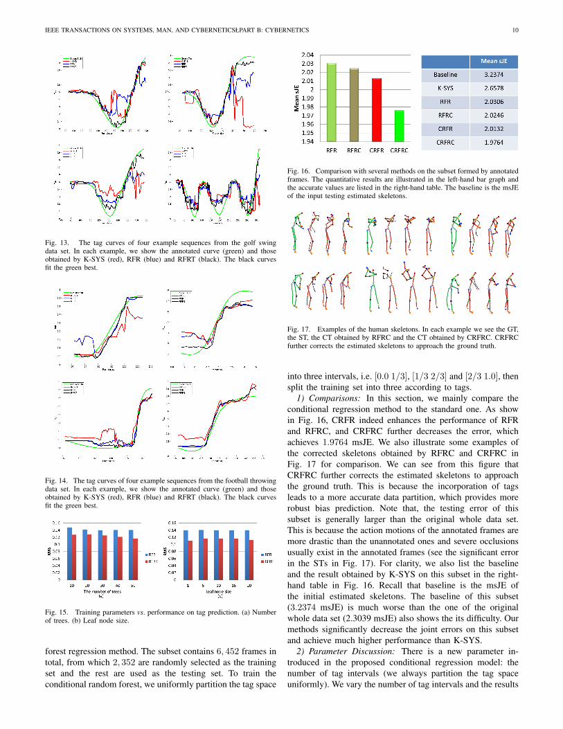
Fig. 16. Comparison with several methods on the subset formed by annotatedframes. The quantitative results are illustrated in the left-hand bar graph andthe accurate values are listed in the right-hand table. The baseline is the msJEof the input testing estimated skeletons.

Fig. 17. Examples of the human skeletons. In each example we see the GT,the ST, the CT obtained by RFRC and the CT obtained by CRFRC. CRFRCfurther corrects the estimated skeletons to approach the ground truth.

into three intervals, i.e. [0.0 1/3], [1/3 2/3] and [2/3 1.0], thensplit the training set into three according to tags.

1) Comparisons: In this section, we mainly compare theconditional regression method to the standard one. As showin Fig. 16, CRFR indeed enhances the performance of RFRand RFRC, and CRFRC further decreases the error, whichachieves 1.9764 msJE. We also illustrate some examples ofthe corrected skeletons obtained by RFRC and CRFRC inFig. 17 for comparison. We can see from this figure thatCRFRC further corrects the estimated skeletons to approachthe ground truth. This is because the incorporation of tagsleads to a more accurate data partition, which provides morerobust bias prediction. Note that, the testing error of thissubset is generally larger than the original whole data set.This is because the action motions of the annotated frames aremore drastic than the unannotated ones and severe occlusionsusually exist in the annotated frames (see the significant errorin the STs in Fig. 17). For clarity, we also list the baselineand the result obtained by K-SYS on this subset in the right-hand table in Fig. 16. Recall that baseline is the msJE ofthe initial estimated skeletons. The baseline of this subset(3.2374 msJE) is much worse than the one of the originalwhole data set (2.3039 msJE) also shows the its difficulty. Ourmethods significantly decrease the joint errors on this subsetand achieve much higher performance than K-SYS.

2) Parameter Discussion: There is a new parameter in-troduced in the proposed conditional regression model: thenumber of tag intervals (we always partition the tag spaceuniformly). We vary the number of tag intervals and the results


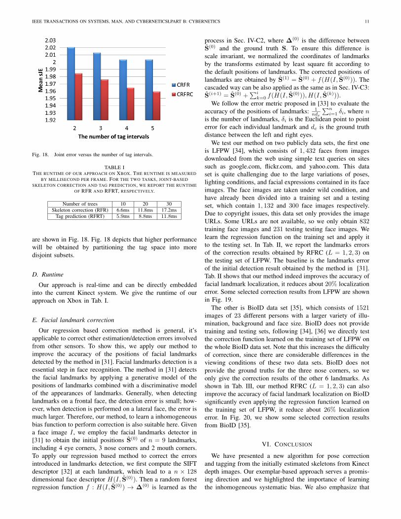
Fig. 18. Joint error versus the number of tag intervals.

TABLE ITHE RUNTIME OF OUR APPROACH ON XBOX. THE RUNTIME IS MEASURED

BY MILLISECOND PER FRAME. FOR THE TWO TASKS, JOINT-BASEDSKELETON CORRECTION AND TAG PREDICTION, WE REPORT THE RUNTIME

OF RFR AND RFRT, RESPECTIVELY.

Number of trees 10 20 30Skeleton correction (RFR) 6.6ms 11.8ms 17.2ms

Tag prediction (RFRT) 5.9ms 8.8ms 11.8ms

are shown in Fig. 18. Fig. 18 depicts that higher performancewill be obtained by partitioning the tag space into moredisjoint subsets.

D. Runtime

Our approach is real-time and can be directly embeddedinto the current Kinect system. We give the runtime of ourapproach on Xbox in Tab. I.

E. Facial landmark correction

Our regression based correction method is general, it’sapplicable to correct other estimation/detection errors involvedfrom other sensors. To show this, we apply our method toimprove the accuracy of the positions of facial landmarksdetected by the method in [31]. Facial landmarks detection is aessential step in face recognition. The method in [31] detectsthe facial landmarks by applying a generative model of thepositions of landmarks combined with a discriminative modelof the appearances of landmarks. Generally, when detectinglandmarks on a frontal face, the detection error is small; how-ever, when detection is performed on a lateral face, the error ismuch larger. Therefore, our method, to learn a inhomogeneousbias function to perform correction is also suitable here. Givena face image I , we employ the facial landmarks detector in[31] to obtain the initial positions S(0) of n = 9 landmarks,including 4 eye corners, 3 nose corners and 2 mouth corners.To apply our regression based method to correct the errorsintroduced in landmarks detection, we first compute the SIFTdescriptor [32] at each landmark, which lead to a n × 128dimensional face descriptor H(I, S(0)). Then a random forestregression function f : H(I, S(0)) → ∆(0) is learned as the

process in Sec. IV-C2, where ∆(0) is the difference betweenS(0) and the ground truth S. To ensure this difference isscale invariant, we normalized the coordinates of landmarksby the transforms estimated by least square fit according tothe default positions of landmarks. The corrected positions oflandmarks are obtained by S(1) = S(0) + f(H(I, S(0))). Thecascaded way can be also applied as the same as in Sec. IV-C3:S(i+1) = S(0) +

∑ik=0 f(H(I, S(0))), H(I, S(k))).

We follow the error metric proposed in [33] to evaluate theaccuracy of the positions of landmarks: 1

nde

∑ni=1 δi, where n

is the number of landmarks, δi is the Euclidean point to pointerror for each individual landmark and de is the ground truthdistance between the left and right eyes.

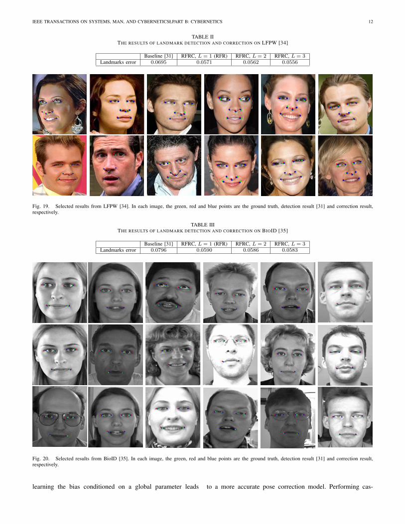
We test our method on two publicly data sets, the first oneis LFPW [34], which consists of 1, 432 faces from imagesdownloaded from the web using simple text queries on sitessuch as google.com, flickr.com, and yahoo.com. This dataset is quite challenging due to the large variations of poses,lighting conditions, and facial expressions contained in its faceimages. The face images are taken under wild condition, andhave already been divided into a training set and a testingset, which contain 1, 132 and 300 face images respectively.Due to copyright issues, this data set only provides the imageURLs. Some URLs are not available, so we only obtain 832training face images and 231 testing testing face images. Welearn the regression function on the training set and apply itto the testing set. In Tab. II, we report the landmarks errorsof the correction results obtained by RFRC (L = 1, 2, 3) onthe testing set of LFPW. The baseline is the landmarks errorof the initial detection result obtained by the method in [31].Tab. II shows that our method indeed improves the accuracy offacial landmark localization, it reduces about 20% localizationerror. Some selected correction results from LFPW are shownin Fig. 19.

The other is BioID data set [35], which consists of 1521images of 23 different persons with a larger variety of illu-mination, background and face size. BioID does not providetraining and testing sets, following [34], [36] we directly testthe correction function learned on the training set of LFPW onthe whole BioID data set. Note that this increases the difficultyof correction, since there are considerable differences in theviewing conditions of these two data sets. BioID does notprovide the ground truths for the three nose corners, so weonly give the correction results of the other 6 landmarks. Asshown in Tab. III, our method RFRC (L = 1, 2, 3) can alsoimprove the accuracy of facial landmark localization on BioIDsignificantly even applying the regression function learned onthe training set of LFPW, it reduce about 26% localizationerror. In Fig. 20, we show some selected correction resultsfrom BioID [35].

VI. CONCLUSION

We have presented a new algorithm for pose correctionand tagging from the initially estimated skeletons from Kinectdepth images. Our exemplar-based approach serves a promis-ing direction and we highlighted the importance of learningthe inhomogeneous systematic bias. We also emphasize that


TABLE IITHE RESULTS OF LANDMARK DETECTION AND CORRECTION ON LFPW [34]

Baseline [31] RFRC, L = 1 (RFR) RFRC, L = 2 RFRC, L = 3Landmarks error 0.0695 0.0571 0.0562 0.0556

Fig. 19. Selected results from LFPW [34]. In each image, the green, red and blue points are the ground truth, detection result [31] and correction result,respectively.

TABLE IIITHE RESULTS OF LANDMARK DETECTION AND CORRECTION ON BIOID [35]

Baseline [31] RFRC, L = 1 (RFR) RFRC, L = 2 RFRC, L = 3Landmarks error 0.0796 0.0590 0.0586 0.0583

Fig. 20. Selected results from BioID [35]. In each image, the green, red and blue points are the ground truth, detection result [31] and correction result,respectively.

learning the bias conditioned on a global parameter leads to a more accurate pose correction model. Performing cas-


caded regression and imposing the temporal consistency alsoimproves pose correction. Our experimental results for bothpose joints correction and tag prediction show significantimprovement over the contemporary systems. Our regressionbased correction method is general, it’s applicable to improvethe accuracy of other detection/estimation systems.

Future works may include designing more powerful skeletalfeatures, employing motion analysis techniques for pose cor-rection and recognizing actions based on the corrected poses.

VII. ACKNOWLEDGEMENTS

This work was supported in part by the National NaturalScience Foundation of China under Grant 61303095 andGrant 61222308, in part by Innovation Program of ShanghaiMunicipal Education Commission under Grant 14YZ018, andin part by the Ministry of Education of China Project NCET-12-0217.

REFERENCES

[1] Microsoft Corp. Kinect for XBOX 360. Redmond WA.[2] L. Liu and L. Shao, “Learning discriminative representations from rgb-d

video data,” in Proc. IJCAI, 2013.[3] J. Shotton, A. Fitzgibbon, M. Cook, T. Sharp, M. Finocchio, R. Moore,

A. Kipman, and A. Blake, “Real-time human pose recognition in partsfrom a single depth image,” in Proc. CVPR, 2011.

[4] R. Girshick, J. Shotton, P. Kohli, A. Criminisi, and A. Fitzgibbon, “Ef-ficient regression of general-activity human poses from depth images,”in Proc. ICCV, 2011.

[5] M. Sun, P. Kohli, and J. Shotton, “Conditional regression forests forhuman pose estimation,” in Proc. CVPR, 2012.

[6] M. Ye, X. Wang, R. Yang, L. Ren, and M. Pollefeys, “Accurate 3d poseestimation from a single depth image,” in Proc. ICCV, 2011.

[7] A. Baak, M. Muller, G. Bharaj, H.-P. Seidel, and C. Theobalt, “A data-driven approach for real-time full body pose reconstruction from a depthcamera,” in Proc. ICCV, 2011.

[8] M. Isard and A. Blake, “Condensation - conditional density propagationfor visual tracking,” Int’l J. of Comp. Vis., vol. 29, no. 1, pp. 5–28, 1998.

[9] D. Comaniciu, V. Ramesh, and P. Meer, “Kernel-based object tracking,”IEEE Trans. PAMI, vol. 25, no. 5, pp. 564–575, 2003.

[10] A. Birnbaum, “A unified theory of estimation,” The Annals of Mathe-matical Statistics, vol. 32, no. 1, 1961.

[11] W. Shen, K. Deng, X. Bai, T. Leyvand, B. Guo, and Z. Tu, “Exemplar-based human action pose correction and tagging,” in Proc. CVPR, 2012.

[12] P. Dollar, V. Rabaud, G. Cottrell, and S. Belongie, “Behavior recognitionvia sparse spatio-temporal features,” in ICCV VS-PETS, 2005.

[13] L. D. Bourdev and J. Malik, “Poselets: Body part detectors trained using3d human pose annotations,” in Proc. ICCV, 2009.

[14] J. C. Niebles, C.-W. Chen, and L. Fei-Fei, “Modeling temporal structureof decomposable motion segments for activity classification,” in Proc.ECCV, 2010.

[15] V. Lepetit, P. Lagger, and P. Fua, “Randomized trees for real-timekeypoint recognition,” in Proc. CVPR, 2005.

[16] J. Han, L. Shao, D. Xu, and J. Shotton, “Enhanced computer vision withmicrosoft kinect sensor: A review,” IEEE Trans. Cybernetics, 2013.

[17] S. Tak and H.-S. Ko, “Physically-based motion retargeting filter,” ACMTransactions on Graphics, vol. 24, no. 1, 2005.

[18] J. Lee and S. Y. Shin, “Motion fairing,” in Proceedings of ComputerAnimation, 1996, pp. 136–143.

[19] H. Lou and J. Chai, “Example-based human motion denoising,” IEEETran. on Visualization and Computer Graphics, vol. 16, no. 5, 2010.

[20] R. Duda, P. Hart, and D. Stork, Pattern Classification and SceneAnalysis. John Wiley and Sons, 2000.

[21] C. E. Rasmussen and C. Williams, Gaussian Processes for MachineLearning. MIT Press, 2006.

[22] B. Scholkopf, A. Smola, R. Williamson, and P. L. Bartlett, “New supportvector algorithms,” Neural Computation, vol. 12, pp. 1207–1245, 2000.

[23] P. Peduzzi, J. Concato, E. Kemper, T. R. Holford, and A. R. Feinstein,“A simulation study of the number of events per variable in logisticregression analysis,” J Clin Epidemiol, vol. 49, no. 12, pp. 1373–1379,1996.

[24] L. Breiman, “Random forests,” Machine Learning, vol. 45, no. 1, pp.5–32, 2001.

[25] J. R. Quinlan, “Induction of decision trees,” Machine Learning, 1986.[26] A. Liaw and M. Wiener, “Classification and regression by randomforest,”

2002.[27] P. Dollar, P. Welinder, and P. Perona, “Cascaded pose regression,” in

Proc. CVPR, 2010.[28] M. Dantone, J. Gall, G. Fanellli, and L. V. Gool, “Real-time facial feature

detection using conditional regression forests,” in Proc. CVPR, 2012.[29] C. E. Rasmussen and H. Nickisch, “Gaussian processes for ma-

chine learning (gpml) toolbox,” Journal of Machine Learning Re-search, vol. 11, pp. 3011–3015, 2010, software available at http://www.gaussianprocess.org/gpml.

[30] C.-C. Chang and C.-J. Lin, “LIBSVM: A library for support vectormachines,” ACM Transactions on Intelligent Systems and Technology,vol. 2, no. 3, pp. 1–27, 2011, software available at http://www.csie.ntu.edu.tw/∼cjlin/libsvm.

[31] M. Everingham, J. Sivic, and A. Zisserman, ““hello! my name is... buffy”- automatic naming of characters in tv video,” in Proc. BMVC, 2006.

[32] C. Liu, J. Yuen, A. Torralba, J. Sivic, and W. T. Freeman, “Sift flow:Dense correspondence across different scenes,” in Proc. ECCV, 2008,pp. 28–42.

[33] D. Cristinacce and T. Cootes, “Feature detection and tracking withconstrained local models,” in Proc. BMVC, 2006.

[34] P. N. Belhumeur, D. W. Jacobs, D. J. Kriegman, and N. Kumar,“Localizing parts of faces using a consensus of exemplars,” in Proc.CVPR, 2011.

[35] O. Jesorsky, K. J. Kirchberg, and R. W. Frischholz, “Robust facedetection using the hausdorff distance,” in Conf. on Audio- and Video-Based Biometric Person Authentication, 2010, pp. 90–95.

[36] X. Cao, Y. Wei, F. Wen, and J. Sun, “Face alignment by explicit shaperegression,” in Proc. CVPR, 2012.

Wei Shen received his B.S. and Ph.D. degree bothin Electronics and Information Engineering fromthe Huazhong University of Science and Technol-ogy (HUST), Wuhan, China, in 2007 and in 2012.From April 2011 to November 2011, he worked inMicrosoft Research Asia as an intern. Now he is afaculty of School of Communication And Informa-tion Engineering, Shanghai University. His researchinterests include computer vision and pattern recog-nition.

Ke Deng received the M.S. degree from TsinghuaUniversity. He is a senior software developmentengineer in Microsoft Corporation.


Xiang Bai received the B.S., M.S., and Ph.D. de-grees from Huazhong University of Science andTechnology (HUST), Wuhan, China, in 2003, 2005,and 2009, respectively, all in electronics and infor-mation engineering. He is currently an AssociateProfessor with the Department of Electronics andInformation Engineering, HUST. From January 2006to May 2007, he was with the Department of Com-puter Science and Information, Temple University,Philadelphia, PA. From October 2007 to October2008, he was with the University of California, Los

Angeles, as a joint Ph.D. student. His research interests include computergraphics, computer vision, and pattern recognition.

Tommer Leyvand received the M.Sc. degree inComputer Science from Tel-Aviv University. Hismain interests include Computer Graphics, Comput-er Vision and Machine Learning. He is a principaldevelopment lead for the XBOX NUI Vision R&Dteam at Microsoft Corporation.

Baining Guo is Deputy Managing Director of Mi-crosoft Research Asia, where he also leads thegraphics lab. Prior to joining Microsoft Researchin 1999, he was a senior staff researcher with theMicrocomputer Research Labs of Intel Corporationin Santa Clara, California. Dr. Guo graduated fromBeijing University with B.S. in mathematics. Heattended Cornell University from 1986 to 1991 andobtained M.S. in Computer Science and Ph.D. inApplied Mathematics. Dr. Guo is a fellow of IEEEand ACM.

Dr. Guo’s research interests include computer graphics, visualization, andnatural user interface. He is particularly interested in studying light trans-mission and reflection in complex, textured materials, with applications totexture and reflectance modeling. He also worked on real-time rendering andgeometry modeling. Dr. Guo was on the editorial boards of IEEE Transactionson Visualization and Computer Graphics (2006–2010) and Computer andGraphics (2007 – 2011). He is currently an associate editor of IEEE ComputerGraphics and Applications. In 2014 he serves as the papers chair for the ACMSIGGRAPH Asia conference. He has served on the program committeesof numerous conferences in graphics and visualization, including ACMSIGGRAPH and IEEE Visualization. Dr. Guo holds over 40 US patents.

Zhuowen Tu received the ME degree from TsinghuaUniversity and the PhD degree from Ohio StateUniversity. He is an assistant professor in the Depart-ment of Cognitive Science, University of California,San Diego (UCSD). Before joining UCSD, he wasan assistant professor at University of California,Los Angeles (UCLA). He was a recipient of theDavid Marr Prize in 2003 and NSF CAREER awardin 2009.

ieee transactions on systems, man, and...

Documents