ieee transactions on power delivery, vol. xx, …caminos.udc.es/gmni/pdf/2007_ieeetpwrd.pdf ·...
TRANSCRIPT
IEEE TRANSACTIONS ON POWER DELIVERY, VOL. XX, NO. Y, MARCH 2006 1
Numerical simulation of transferred potentials inearthing grids considering layered soil models
I. Colominas, F. Navarrina, M. Casteleiro
Abstract
Computing the potential distribution on the earth surfacewhen a fault condition occurs is essential to assure the securityof the grounding systems in electrical substations.
This paper presents a numerical formulation for the analysisof transferred earth potentials in a grounding installation dueto metallic stuctures or conductors in the surroundings of thegrounding grid when a layered soil model is considered [1].This transference of potentials between the grounding area todistant points by buried conductors, such as communication orsignal circuits, neutral wires, pipes, rails, or metallic fences,may produce serious safety problems. The authors have re-cently developed a numerical technique based on the Bound-ary Element Method for the analysis of transferred earth poten-tials in the case of uniform soil models [2]. In this work, it ispresented its generalization for a two layer soil model. Thus,the main highlights of the numerical approach are summarizedand some examples by using the geometry of real groundingsystems in different cases of transferred potentials consideringdifferent soil models are presented.
Keywords: Grounding Analysis, Two Layer Soil Model,Transferred Earth Potential, Boundary Element Method
I. INTRODUCTION
A safe grounding system has to guarantee the integrity ofequipment and the continuity of the service under fault condi-tions —providing means to carry and dissipate electrical cur-rents into the ground— and to safeguard that persons workingor walking in the surroundings of the grounded installation arenot exposed to dangerous electrical shocks. To achieve thesegoals, the equivalent electrical resistance of the system mustbe low enough to assure that fault currents dissipate mainlythrough the grounding grid into the earth, while maximum po-tential differences between close points on the earth surfacemust be kept under certain tolerances, defined by the step, touchand mesh voltages [1], [3].
Equations which govern the well-known phenomenon of theelectrical current dissipation into a soil can be stated by meansof Maxwell’s Electromagnetic Theory [4]. However their ap-plication and resolution for the computing of grounding grids
I. Colominas, F. Navarrina and M. Casteleiro serve at the Dept. of AppliedMath., Civil Engrg. School, Univ. of A Coruna, Campus de Elvina. 15071 ACoruna, SPAIN. (e-mail: [email protected])
of large electrical substations in practical cases present somedifficulties: No analytical solutions can be obtained for mostof real problems, and the use of standard numerical methods(such as finite elements or finite differences) is very difficult dueto the specific geometry of the grounding grids in main earth-ing systems (a mesh of interconnected bare conductors with arelatively small ratio diameter-length). These methods shouldrequire an extremely costly discretization of the domain (theground excluding the electrode), and therefore obtaining suffi-ciently accurate results should imply unacceptable computingefforts in memory storage and CPU time.
In the last years, the authors have proposed a numerical ap-proach based on the transformation of the Maxwell’s differen-tial equations onto an equivalent boundary integral equation [4].Thus, the statement of a variational form based on a weighted-residual approach of the boundary integral equation and the se-lection of a Galerkin type weighting lead to a general symmetricformulation [5]. The subsequent application of the BoundaryElement Method [6] allows to derive specific numerical algo-rithms of high accuracy for the analysis of grounding systemsembedded in uniform soils models [5]. Besides, it is possi-ble to explain rigorously the anomalous asymptotic behaviourof the clasical methods proposed for grounding analyis, and toidentify the sources of error [4]. Finally, this boundary elementformulation has been recently extended for grounding grids em-bedded in layered soils [7], [8].
In 2005, the authors proposed a methodology for the analy-sis of a common and very important engineering problem in thegrounding field: the problem of transferred earth potentials bygrounding grids [2]. This first work was limited to the trans-ferred potential analysis by considering uniform soil models.In this paper, it is presented the generalization of this numericalmethodology to layered soil models.
II. NUMERICAL MODEL OF THE PROBLEM OF THE
CURRENT DISSIPATION INTO A LAYERED SOIL
Restricting the analysis to the electrokinetic steady-state re-sponse and neglecting the inner resistivity of the earthing con-ductors (therefore, potential can be assumed constant at everypoint of the grounding electrode surface), the problem of theelectrical dissipation current into a soil can be written in termsof the 3D problem
div���������������� � �� �������������� � ��������������� grad�� � in �������������������������������� � � in ��� � � �� in �� � � �� if ���������������� � � (1)
where� is the earth, �������������� is its conductivity tensor, �� is the earthsurface,��������������� is its normal exterior unit field and� is the electrodesurface [1], [5].
IEEE TRANSACTIONS ON POWER DELIVERY, VOL. XX, NO. Y, MARCH 2006 2
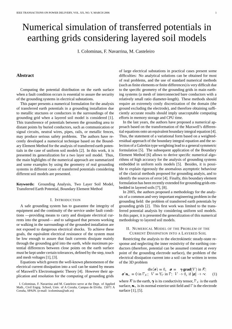
Fig. 1. Fault current disipation in a stratified soil model.
The solution to problem (1) gives the potential � and the cur-rent density �������������� at an arbitrary point �������������� when the electrode attainsa voltage �� (Ground Potential Rise, or GPR) with respect to aremote earth. Next, for known values of � on �� and �������������� on �,it is straightforward to obtain the design and safety parametersof the grounding system [5], [8].
Different approaches can be stated depending on the soilmodel. The simplest one is the homogeneous and isotropic soilmodel where the conductivity tensor �������������� can be substituted by anapparent scalar conductivity � that must be experimentally ob-tained [1], [4], [5]. This kind of soil model is advisable whenthe soil is basically uniform in the horizontal and vertical di-rections or if the resistivity varies slightly with depth. In othercases, it is more convenient to develop more accurate models toconsider the major variations in the soil conductivity.
Evidently, since taking into account all changes in the soilconductivity is unaffordable, a more practical soil models havebeen proposed specially when conductivity is not markedly uni-form with depth: the “layered soil” models. These models con-sist of considering the soil stratified in a number of horizontallayers, each one defined by a thickness and an apparent scalarconductivity. In fact, it is widely accepted that two-layer (oreven three-layer) soil models should be sufficient to obtain goodand safe designs of grounding systems in most practical cases[1], [9], [10]. In this point, it is important to notice that, inpractice, the surroundings of the substations site are levelledand regularized during its construction; therefore all layers canbe really assumed horizontal, and even the earth surface.
For a general case of a soil model formed by � horizontallayers (each one with a different conductivity) with the ground-ing electrode buried in the layer , the mathematical problem(1) can be written in terms of the following Neumann exteriorproblem
div����������������� � �� ��������������� � ��� gradgradgradgradgradgradgradgradgradgradgradgradgradgrad���� in ��� � � � ��������������������������������� � � in �� � �� � �� in �� �� � � if ���������������� � ��
������������������������������� � ��������������������������������� in��� � � � � � � (2)
being �� each one of the soil layer � � �� ��, �������� theinterphase between whatever two layers ( � � and ), �� thescalar conductivity of layer , �� the potential at every pointof layer and ��������������� its current density [11], [12], [13] (see Fig.1). Since the problem is linear, the boundary condition � � ��� in � can be substituted by a unitary one �� � � in �, andlater, scaling up all results.
As we have previously exposed, the specific geometry ofthe grounding grids in practice greatly complicates to solve theequations of problem (2) for the huge effort necessary for thediscretization of the domain, being virtually impossible to solve(2) by means of numerical techniques widely used in computa-tional design in engineering (such as the Finite Element Methodor the Finite Difference Method). For this reason, we haveturned our attention to other numerical methods (based on theBoundary Element Method) which only require the discretiza-tion of the boundary of the problem (that is, the surface of theelectrodes). However, the application of these methods firstlyrequires obtaining an integral expression for the potential interms of unknowns defined on the boundaries [5], [8]. Thus, theapplication of the “method of images” and the Green’s Identityto (2) leads to the following integral expression for potential������������������� at an arbitrary point ��������������� � ��, in terms of the leakagecurrent density ����������������� that flows from any point �������������� on the elec-trode surface � � �� (� � �����������������������������, where �������������� is the normal exteriorunit field to �):
�������������������������������� ��
����
� �����������������
������������������� ����������������������������������� ���������������� � ��� (3)
The integral kernels ������������������� ��������������� are series of terms correspond-ing to the resultant images, which number shall be finite or in-finite depending on the soil model considered [1], [11]. Gener-ally speaking, the integral kernels depend on the thickness andconductivity of each layer and on the inverse of the distancesfrom the point ��������������� to the point �������������� and to all the symmetric pointsof �������������� (its images) with respect to the earth surface �� and to theinterphases �������� between layers [11], [13].
Although generation of electrical images in a general caseis a conceptually simple well-known process [14], the final ex-pression of the integral kernels ������������������� ��������������� can be very compli-cated, and its evaluation in practice may require a high com-puting effort. In the appendix I, it can be found the explicitexpressions of the integral kernels for one-layer and two-layersoil models.
On the other hand, since integral expression (3) also verifieson �, where the potential is given by the boundary condition������������������ � �, ��������������� � �, the leakage current density � must satisfy
�
����
������������������
������������������ �������������������������������� �� � �� ��������������� � �� (4)
Now, the application of the weighted residuals method to theequation (4) allows to obtain the variational statement
������������������
�����������������
��
����
������������������
������������������ �������������������������������� ��� �
��� � ��
(5)

IEEE TRANSACTIONS ON POWER DELIVERY, VOL. XX, NO. Y, MARCH 2006 3
for all members � of a suitable class of test functions ����������������� de-fined on � [5], [8]. Now, since the unknown function (the leak-age current density) is defined on the boundary of the domain,a numerical approach based on the Boundary Element Method[6] should be clearly the right election for solving the integralequation (5).
The complete development of the numerical approach forlayered soil models and an in-depth discussion, including sev-eral application examples, can be found in references [7], [8],[13]. Next, it is presented the fundamentals of the numericalformulation based on the Boundary Element Method for solv-ing equation (5) and for computing potential by means of (3).
First of all, the development of the numerical model requiresthe discretization of the leakage current density � in terms ofa set of trial functions, and the discretization of the electrodesurface � in terms of a set of boundary elements:
����������������� ������������������ ������
��������������������� � � �
���
�� (6)
Consequently, the potential ������������������� given by (3) can be dis-cretized as
�������������������������������� �
�����
��� ��������������������� ���
����������������� �
���
� �������������������� (7)
where � ��
depends on the integral on the boundary element of
the integral kernel �� multiplies by the trial function [8].Likewise, given a set of test functions defined on �, the inte-
gral equation (5) can be discretized leading to a linear systemof equations
�����
������ � �� � � �� � � � � � � (8)
where ��� depends on the double integrals on the boundary el-ements of the integral kernel �� multiply by the trial and testfunctions, and ��� depends on the integral on the boundary ele-ment of the test function [5].
The solution of this system of linear equations is the key ofthe problem because it provides the values of the unknowns��� �� � �� � � � � �� that are necessary to compute the potential�� at any point ��������������� by means of (7). From the leakage currentdensity �, it is straightforward to obtain other safety parametersfor grounding design [5].
The boundary element numerical formulation for groundinganalysis is completely developed in [5], [8]. In these references,it can also be found the derivation of a 1D approximated nu-merical approach that takes into account the real geometry ofgrounding systems in practical cases, and the highly efficientanalytical integration techniques developed by the authors forcomputing the integral terms required in (7) and (8).
Furthermore, in references [4], [5], one can find a fully ex-plicit discussion about the main numerical aspects of the BEMnumerical approaches, such as the asymptotic convergence, theoverall computational efficiency, and the complete explanationof the sources of error of the widespread intuitive methods. And
�
�
��
��
��
��
���
���
���
�� �� ��
GROUNDING GRID
��
Fig. 2. Plan of the grounding grid of the electrical substation buried to a depthof 0.8m.
in references [15], [16], it can be found a comparison and a val-idation of the BEM approach with other numerical techniques(like a Finite Element analysis among others methods).
This approach is highly efficient from a computational pointof view, and it has been implemented in a CAD system forgrounding analysis in layered soil models [4], [5], [8], [17].Examples presented in this paper correspond to cases with uni-form and two-layers soil models. Obviously, this BEM formu-lation could be applied to other cases with a higher number oflayers. However, it is important to take into account that thecomputing time may considerably increase, mainly because oftwo facts which are not strictly related to the numerical formu-lation: a) the complexity of the kernels in the integral expres-sion of potential (3) obtained by application of the method ofimages (usually a multiple infinite series); and b) the high num-ber of terms of these series that must be evaluated especiallywhen conductivities between layers are very different.
In the next section, it is presented a methodology for the anal-ysis of transferred earth potentials in grounding systems if lay-ered soil models are considered by using the above numericalmethod.

IEEE TRANSACTIONS ON POWER DELIVERY, VOL. XX, NO. Y, MARCH 2006 4
III. ANALYSIS OF TRANSFERRED EARTH POTENTIALS IN
LAYERED SOIL MODELS
As it is well-known, “transferred earth potentials” refe r tothe phenomenon of the earth potential of one location appear-ing at another location with a contrasting earth potential [18].This transference occurs, for example, when a grounding grid isenergized up to a certain voltage (the GPR) during a fault con-dition, and this voltage (or a fraction of it) is transferred out to anon-fault site by a ground conductor: metal pipes, rails, metal-lic fences, etc., leaving the substation area. It is obvious thedanger that can imply this potential transference to people, ani-mals or the equipment [19], especially because in some cases itis produced in unexpected and non-protected areas.
Avoiding transferred potentials is not always possible: thisphenomenon can be produced for example by the railroad trackswhich are often used in large substations to install high-powertransformers or other large equipment [20]. The prevention ofthese hazardous voltages is generally performed combining agood engineering expertise, some very crude calculations andeven field measurements [1], [19], [20], [21], [22].
At present, a more accurate determination of the transferredearth potentials can be carried out by using computer methodsfor grounding analysis. In a previous work [2], the authors pro-posed a methodology limited to the case of uniform soil mod-els. Now, we propose its generalization for layered soil modelsbased on the boundary element numerical approach previouslypresented.
The analysis of transferred earth potentials is especially com-plicated if the grounding grid and the other extra-conductors arenot electrically interconnected (that is the more frequent anddangerous case), since these conductors are energized to an un-known fraction of the GPR when a fault condition occurs.
The key idea to obtain this voltage (and from it, the rest ofthe safety parameters of the grounding system) lies in that theelectrodes of the grounding grid form an “active grid” (whichis leaking into the soil an unknown total current � ), while theextra-conductors make up a “passive grid” (which is leaking nocurrent into the soil).
Since the state equations are linear, the analysis of transferredpotentials from the “active” to the “passive” grid can be math-ematically performed by means of a superposition of two ele-mentary states: 1) the “active grid” energized to 1 V and the“passive grid” to 0 V; and 2) the “active grid” energized to 0 Vand the “passive grid” energized to 1 V.
Each elementary state is solved by means of the boundaryelement numerical approach of section II with the layered soilmodel considered, obtaining the total electrical currents by unitof voltage which flow from each “grid”: ���, ���, �� and ��(“A” refers to the “active grid”, “P” refers to the “passive grid”,and the numbers refer to each elementary state).
But in practice, the real state is formed by the “active grid”energized to the GPR and the “passive grid” to an unknownfraction � of the GPR, that is, the superposition of the elemen-tary state 1) weighted by the GPR of the “active grid” (��) andthe state 2) weighted by a fraction of the GPR (���).
Once the total electrical currents per unit of voltage are ob-tained, the coefficient � and the total fault current being leakedinto the soil � are computed taking into account that the fault
�
�
��
��
��
��
���
���
���
�� �� �� ��
2 RAILS
half-buried
GROUNDING GRID
Fig. 3. Plan of the grounding grid of the electrical substation (buried to a depthof 0.8m) and the two railway tracks (buried to a depth of 0.1m).
currents are only derived through the grounding grid, and thatno current is leaked by the extra-conductors [2], [15]; that is,by solving the linear system of equations,
� � �� ��� ��� ���� � �� �� ��� ��� (9)
Finally, it is possible to obtain the equivalent resistance ofthe grounding system and the potential distribution on the earthsurface at any point of the substation site and of its surround-ings, once the total fault current � and the fraction � of theGPR are computed.
The feasibility of this methodology will be demonstrated inthe next section with some application examples of transferredearth analysis of a grounding grid by considering uniform andtwo-layer soil models.
IV. EXAMPLE OF TRANSFERRED POTENTIAL ANALYSIS
CONSIDERING DIFFERENT SOIL MODELS. DISCUSSION
In this section we present the analysis of the transferred earthpotentials by railway tracks close to the grounding system ofan electrical substation considering different type of soil mod-els. With the aim of proving the feasibility of the proposed nu-merical approach in a practical case, we have been chosen thegeometry of a real grounding grid (the plan is shown in Figure

IEEE TRANSACTIONS ON POWER DELIVERY, VOL. XX, NO. Y, MARCH 2006 5
TABLE IGROUNDING SYSTEM: CHARACTERISTICS
DataNumber of electrodes: 408Diameter of electrodes: 12.85 mmDepth of the grid: 0.80 mMax. dimensions of grid: 14590 m�
TABLE IIRAILWAY TRACKS: CHARACTERISTICS
DataNumber of tracks: 2Length of the tracks: 130 mDistance between the tracks: 1668 mmDiameter of the tracks: 94 mmDepth: 100 mm
2). The earthing grid is formed by a mesh of 408 cylindricalconductors buried to a depth of 0.80 m (see Table I).
On the other hand, the same grounding system has been an-alyzed but now considering the existence of two railway tracksin the surroundings. This is a common situation in electricalsubstations and generating plants where a railway spur is usedfor the installation of large equipment during the constructionphase of the electrical installation, fuel supplying, etc. [20].The characteristics and dimensions of the tracks are given inTable II, while the plan of the earthing grid including the tracksis given in Figure 3.
In all examples presented in this paper, we have considered aGround Potential Rise (GPR) of 10 kV.
We have studied both earthing systems (Fig. 2 and Fig. 3) byconsidering three different type of soil models.
In the first case (Case 1) we have considered a one layer soilmodel, that is, a homogeneous and isotropic soil model with anapparent scalar resistivity of 50 m. Table III summarizes thenumerical model data and some results: the total fault current,the equivalent resistance and the ratio of transferred potentials(�). Case 1A refers to the grounding grid analysis (Fig. 2), andCase 1B refers to the analysis of grounding transferred poten-tials for the railway tracks (Fig. 3).
The potential distribution on the earth surface when a faultcondition occurs is shown in Figures 4 and 5 for Case 1A and1B, respectively.
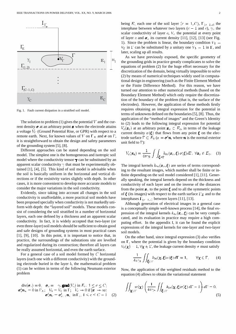
The second case (Case 2) corresponds to a layered soil modelformed by two horizontal strata: the upper one with an appar-ent scalar resistivity of 50 m and a thickness of 1.2m, and thelower one with an apparent scalar resistivity of 500 m. Ta-ble IV summarizes the numerical model data and some results:the total fault current, the equivalent resistance and the ratio oftransferred potentials (�). Case 2A refers to the grounding gridanalysis (Fig. 2), and Case 2B refers to the analysis of ground-ing transferred potentials for the railway tracks (Fig. 3).
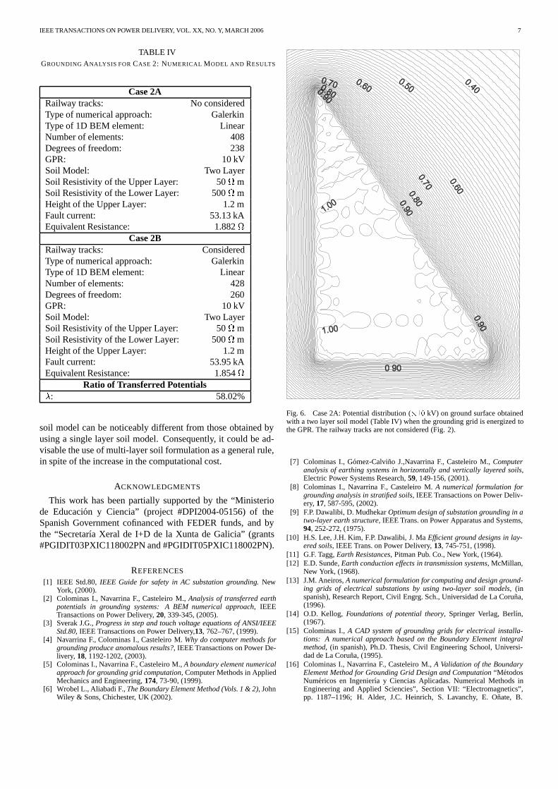
The potential distribution on the earth surface when a faultcondition occurs is shown in Figures 6 and 7 for Case 2A and2B, respectively.
TABLE IIIGROUNDING ANALYSIS FOR CASE 1: NUMERICAL MODEL AND RESULTS
Case 1ARailway tracks: No consideredType of numerical approach: GalerkinType of 1D BEM element: LinearNumber of elements: 408Degrees of freedom: 238GPR: 10 kVSoil Model: One LayerSoil Resistivity: 50 mFault current: 38.12 kAEquivalent Resistance: 0.2623
Case 1BRailway tracks: ConsideredType of numerical approach: GalerkinType of 1D BEM element: LinearNumber of elements: 428Degrees of freedom: 260GPR: 10 kVSoil Model: One LayerSoil Resistivity: 50 mFault current: 38.28 kAEquivalent Resistance: 0.2613
Ratio of Transferred Potentials�: 42.33%
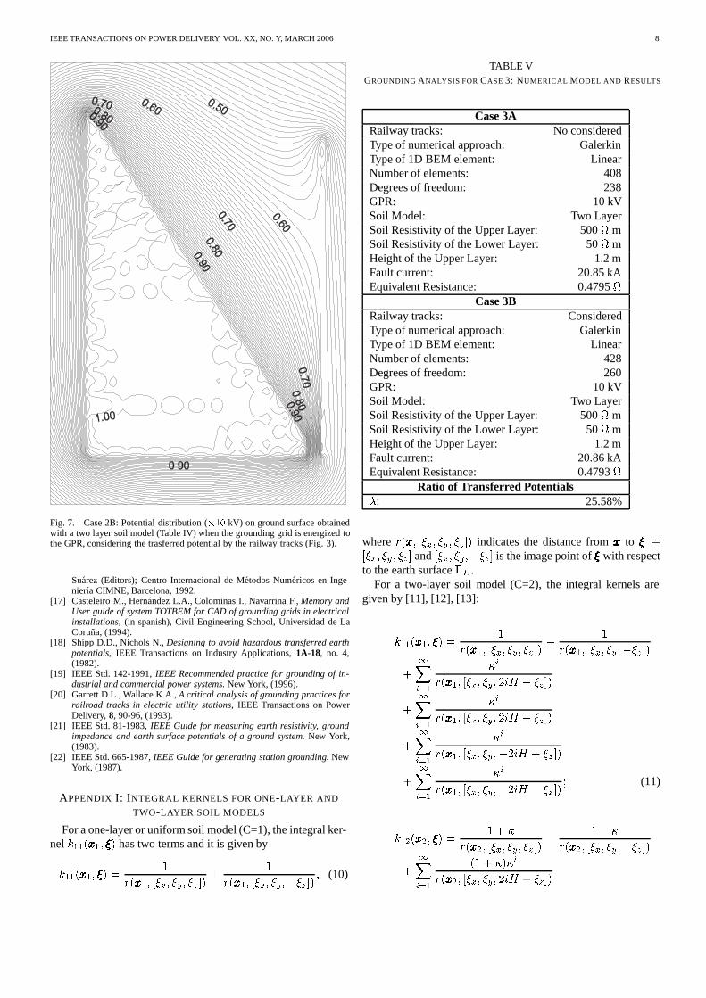
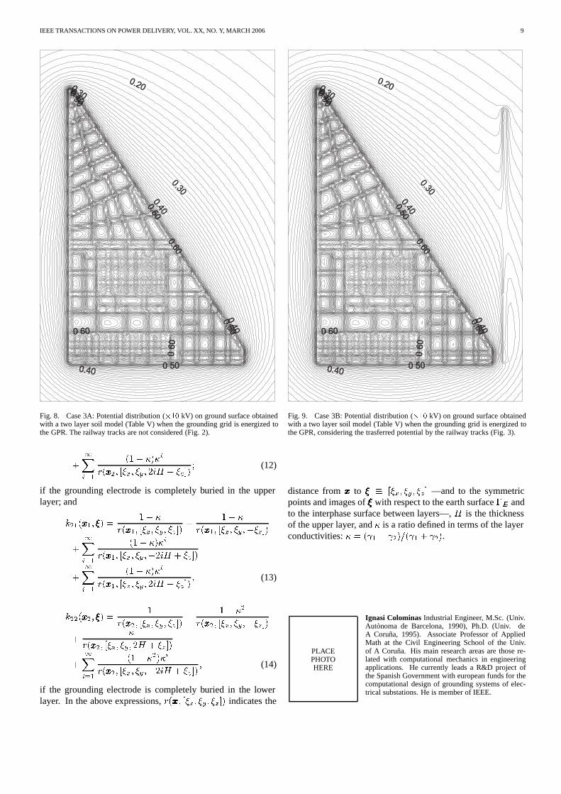
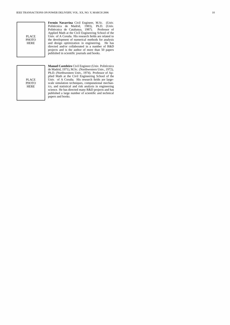
Finally, we have considered a third case (Case 3) also corre-sponding to a two layer soil model formed by an upper stratumwith an apparent scalar resistivity of 500 m and a thicknessof 1.2m, and a lower stratum with an apparent scalar resistiv-ity of 50 m. Table V summarizes the numerical model dataand some results: the total fault current, the equivalent resis-tance and the ratio of transferred potentials (�). Case 3A refersto the grounding grid analysis (Fig. 2), and Case 3B refers tothe analysis of grounding transferred potentials for the railwaytracks (Fig. 3).
The potential distribution on the earth surface when a faultcondition occurs is shown in Figures 8 and 9 for Case 3A and3B, respectively.
As it can be observed, there are significant differences in thepotential distribution on the earth surface and in the equivalentresistance depending on the soil model considered. Thus, forexample, the equivalent resistance varies from� ���� for theuniform model, to � �� for the two-layer soil model of case2, or � ���� for the two-layer soil model of case 3.
For each particular case, the differences in the equivalent re-sistance of the earhing system are insignificant: 0.2623 and0.2613 for the uniform model; 1.882 and 1.854 for thecase 2; and 0.4795 and 0.4793 for the case 3, since evi-dently the contribution of the tracks to the electrical resistanceof the global earthing system should be irrelevant (specially, be-cause there is no electrical link between the grounding grid andthem).
On the other hand, and also for each particular case, it isobvious that there are only slightly differences in the poten-

IEEE TRANSACTIONS ON POWER DELIVERY, VOL. XX, NO. Y, MARCH 2006 6
Fig. 4. Case 1A: Potential distribution (��� kV) on ground surface obtainedwith a homogeneous and isotropic soil model (Table III) when the groundinggrid is energized to the GPR. The railway tracks are not considered (Fig. 2).
tial distribution on the earth surface in the area covered by thegrounding grid of the electrical substation (figures 4 and 5, forcase 1; figures 6 and 7, for case 2; and figres 8 and 9, for case3). Nevertheless, the most important differences in the poten-tial distribution on the earth surface can be observed speciallyin the surroundings of the railway tracks, where important po-tential gradients are produced: in some points in the vicinity ofthe tracks, the computed step voltages are ten times higher thanthe computed step voltages without considering the transferredpotentials by the tracks. This situation is particularly hazardousbecause it is produced far away from the substation site, andprobably in a non-protected area.
In the presented examples, we show that the results obtainedby using a multiple-layer soil model can be noticeably differentfrom those obtained by using a single layer soil model. And notonly the general design parameters of a grounding system (suchas the equivalent resistance, the touch voltage, the step voltage,the mesh voltage, etc.) will significantly vary, but the results ofthe transferred earth analysis will be also substantially differ-ent. Therefore, it could be advisable to use efficient multi-layersoil formulations —such as the numerical approach presentedin this paper— to analyze grounding systems and transferred
Fig. 5. Case 1B: Potential distribution (��� kV) on ground surface obtainedwith a homogeneous and isotropic soil model (Table III) when the groundinggrid is energized to the GPR, considering the trasferred potential by the railwaytracks (Fig. 3).
earth potential effects as a general rule, in spite of the increasein the computational effort. In fact, the use of this kind of ad-vanced models should be mandatory in cases where the conduc-tivity of the soil changes markedly with depth.
V. CONCLUSIONS
In this paper, the mathematical model of the physical phe-nomenon of the electrical current dissipation through a ground-ing grid into a stratified soil has been revised, and it has beenpresented the main highlights of a numerical formulation basedon the Boundary Element Method proposed by the authors forgrounding analysis in uniform and two-layer soil models.
This boundary element approach has turned out to be a gen-eral framework for the computational analysis of transferredearth potentials by electrical conductors buried in the surround-ings of a grounding system. Three main cases of transferredearth potentials have been analyzed: one case with a uniformsoil model, and two cases with a 2-layer soil models.
It has been shown that highly accurate results can be obtainedby means of the proposed methodology in the earthing analysisof real problems, and how results obtained by using a two-layer
IEEE TRANSACTIONS ON POWER DELIVERY, VOL. XX, NO. Y, MARCH 2006 7
TABLE IVGROUNDING ANALYSIS FOR CASE 2: NUMERICAL MODEL AND RESULTS
Case 2ARailway tracks: No consideredType of numerical approach: GalerkinType of 1D BEM element: LinearNumber of elements: 408Degrees of freedom: 238GPR: 10 kVSoil Model: Two LayerSoil Resistivity of the Upper Layer: 50 mSoil Resistivity of the Lower Layer: 500 mHeight of the Upper Layer: 1.2 mFault current: 53.13 kAEquivalent Resistance: 1.882
Case 2BRailway tracks: ConsideredType of numerical approach: GalerkinType of 1D BEM element: LinearNumber of elements: 428Degrees of freedom: 260GPR: 10 kVSoil Model: Two LayerSoil Resistivity of the Upper Layer: 50 mSoil Resistivity of the Lower Layer: 500 mHeight of the Upper Layer: 1.2 mFault current: 53.95 kAEquivalent Resistance: 1.854
Ratio of Transferred Potentials�: 58.02%
soil model can be noticeably different from those obtained byusing a single layer soil model. Consequently, it could be ad-visable the use of multi-layer soil formulation as a general rule,in spite of the increase in the computational cost.
ACKNOWLEDGMENTS
This work has been partially supported by the “Ministeriode Educacion y Ciencia” (project #DPI2004-05156) of theSpanish Government cofinanced with FEDER funds, and bythe “Secretarıa Xeral de I+D de la Xunta de Galicia” (grants#PGIDIT03PXIC118002PN and #PGIDIT05PXIC118002PN).
REFERENCES
[1] IEEE Std.80, IEEE Guide for safety in AC substation grounding. NewYork, (2000).
[2] Colominas I., Navarrina F., Casteleiro M., Analysis of transferred earthpotentials in grounding systems: A BEM numerical approach, IEEETransactions on Power Delivery, 20, 339-345, (2005).
[3] Sverak J.G., Progress in step and touch voltage equations of ANSI/IEEEStd.80, IEEE Transactions on Power Delivery,13, 762–767, (1999).
[4] Navarrina F., Colominas I., Casteleiro M. Why do computer methods forgrounding produce anomalous results?, IEEE Transactions on Power De-livery, 18, 1192-1202, (2003).
[5] Colominas I., Navarrina F., Casteleiro M., A boundary element numericalapproach for grounding grid computation, Computer Methods in AppliedMechanics and Engineering, 174, 73-90, (1999).
[6] Wrobel L., Aliabadi F., The Boundary Element Method (Vols. 1 & 2), JohnWiley & Sons, Chichester, UK (2002).
Fig. 6. Case 2A: Potential distribution (��� kV) on ground surface obtainedwith a two layer soil model (Table IV) when the grounding grid is energized tothe GPR. The railway tracks are not considered (Fig. 2).
[7] Colominas I., Gomez-Calvino J.,Navarrina F., Casteleiro M., Computeranalysis of earthing systems in horizontally and vertically layered soils,Electric Power Systems Research, 59, 149-156, (2001).
[8] Colominas I., Navarrina F., Casteleiro M. A numerical formulation forgrounding analysis in stratified soils, IEEE Transactions on Power Deliv-ery, 17, 587-595, (2002).
[9] F.P. Dawalibi, D. Mudhekar Optimum design of substation grounding in atwo-layer earth structure, IEEE Trans. on Power Apparatus and Systems,94, 252-272, (1975).
[10] H.S. Lee, J.H. Kim, F.P. Dawalibi, J. Ma Efficient ground designs in lay-ered soils, IEEE Trans. on Power Delivery, 13, 745-751, (1998).
[11] G.F. Tagg, Earth Resistances, Pitman Pub. Co., New York, (1964).[12] E.D. Sunde, Earth conduction effects in transmission systems, McMillan,
New York, (1968).[13] J.M. Aneiros, A numerical formulation for computing and design ground-
ing grids of electrical substations by using two-layer soil models, (inspanish), Research Report, Civil Engrg. Sch., Universidad de La Coruna,(1996).
[14] O.D. Kellog, Foundations of potential theory, Springer Verlag, Berlın,(1967).
[15] Colominas I., A CAD system of grounding grids for electrical installa-tions: A numerical approach based on the Boundary Element integralmethod, (in spanish), Ph.D. Thesis, Civil Engineering School, Universi-dad de La Coruna, (1995).
[16] Colominas I., Navarrina F., Casteleiro M., A Validation of the BoundaryElement Method for Grounding Grid Design and Computation “MetodosNumericos en Ingenierıa y Ciencias Aplicadas. Numerical Methods inEngineering and Applied Sciencies”, Section VII: “Electromagnetics”,pp. 1187–1196; H. Alder, J.C. Heinrich, S. Lavanchy, E. Onate, B.
IEEE TRANSACTIONS ON POWER DELIVERY, VOL. XX, NO. Y, MARCH 2006 8
Fig. 7. Case 2B: Potential distribution (��� kV) on ground surface obtainedwith a two layer soil model (Table IV) when the grounding grid is energized tothe GPR, considering the trasferred potential by the railway tracks (Fig. 3).
Suarez (Editors); Centro Internacional de Metodos Numericos en Inge-nierıa CIMNE, Barcelona, 1992.
[17] Casteleiro M., Hernandez L.A., Colominas I., Navarrina F., Memory andUser guide of system TOTBEM for CAD of grounding grids in electricalinstallations, (in spanish), Civil Engineering School, Universidad de LaCoruna, (1994).
[18] Shipp D.D., Nichols N., Designing to avoid hazardous transferred earthpotentials, IEEE Transactions on Industry Applications, 1A-18, no. 4,(1982).
[19] IEEE Std. 142-1991, IEEE Recommended practice for grounding of in-dustrial and commercial power systems. New York, (1996).
[20] Garrett D.L., Wallace K.A., A critical analysis of grounding practices forrailroad tracks in electric utility stations, IEEE Transactions on PowerDelivery, 8, 90-96, (1993).
[21] IEEE Std. 81-1983, IEEE Guide for measuring earth resistivity, groundimpedance and earth surface potentials of a ground system. New York,(1983).
[22] IEEE Std. 665-1987, IEEE Guide for generating station grounding. NewYork, (1987).
APPENDIX I: INTEGRAL KERNELS FOR ONE-LAYER AND
TWO-LAYER SOIL MODELS
For a one-layer or uniform soil model (C=1), the integral ker-nel ������������������� ��������������� has two terms and it is given by
������������������� ��������������� ��
������������������ ���� ��� ����
�
������������������ ���� ��������� (10)
TABLE VGROUNDING ANALYSIS FOR CASE 3: NUMERICAL MODEL AND RESULTS
Case 3ARailway tracks: No consideredType of numerical approach: GalerkinType of 1D BEM element: LinearNumber of elements: 408Degrees of freedom: 238GPR: 10 kVSoil Model: Two LayerSoil Resistivity of the Upper Layer: 500 mSoil Resistivity of the Lower Layer: 50 mHeight of the Upper Layer: 1.2 mFault current: 20.85 kAEquivalent Resistance: 0.4795
Case 3BRailway tracks: ConsideredType of numerical approach: GalerkinType of 1D BEM element: LinearNumber of elements: 428Degrees of freedom: 260GPR: 10 kVSoil Model: Two LayerSoil Resistivity of the Upper Layer: 500 mSoil Resistivity of the Lower Layer: 50 mHeight of the Upper Layer: 1.2 mFault current: 20.86 kAEquivalent Resistance: 0.4793
Ratio of Transferred Potentials�: 25.58%
where ����������������� ���� ��� ���� indicates the distance from �������������� to �������������� ����� ��� ��� and ���� ������� is the image point of �������������� with respectto the earth surface �� .
For a two-layer soil model (C=2), the integral kernels aregiven by [11], [12], [13]:
������������������� ��������������� ��
������������������ ���� ��� �� ��
�
������������������ ���� ������ ��
�����
��
������������������ ���� ��� ��� ����
�����
��
������������������ ���� ��� ��� � ����
�����
��
������������������ ���� ������� �� ��
�����
��
������������������ ���� ������� � �� ��� (11)
������������������� ��������������� �� �
������������������ ���� ��� �� ��
� �
������������������ ���� ������ ��
�����
�� ����
������������������ ���� ��� ��� ����
IEEE TRANSACTIONS ON POWER DELIVERY, VOL. XX, NO. Y, MARCH 2006 9
Fig. 8. Case 3A: Potential distribution (��� kV) on ground surface obtainedwith a two layer soil model (Table V) when the grounding grid is energized tothe GPR. The railway tracks are not considered (Fig. 2).
�����
�� ����
������������������ ���� ��� ��� � ����� (12)
if the grounding electrode is completely buried in the upperlayer; and
������������������� ��������������� ��� �
������������������ ���� �� � ����
�� �
������������������ ���� ��������
�����
��� ����
������������������ ���� ������� �� ��
�����
��� ����
������������������ ���� ��� ��� � ����� (13)
������������������� ��������������� ��
������������������ ���� �� � ����
�� ��
������������������ ���� ��������
��
������������������ ���� ��� �� ����
�����
��� �����
������������������ ���� ������� �� ��� (14)
if the grounding electrode is completely buried in the lowerlayer. In the above expressions, ����������������� ���� ��� ���� indicates the
Fig. 9. Case 3B: Potential distribution (��� kV) on ground surface obtainedwith a two layer soil model (Table V) when the grounding grid is energized tothe GPR, considering the trasferred potential by the railway tracks (Fig. 3).
distance from �������������� to �������������� � ���� ��� ��� —and to the symmetricpoints and images of �������������� with respect to the earth surface �� andto the interphase surface between layers—, � is the thicknessof the upper layer, and � is a ratio defined in terms of the layerconductivities: � � ��� � ������� ���.
PLACEPHOTOHERE
Ignasi Colominas Industrial Engineer, M.Sc. (Univ.Autonoma de Barcelona, 1990), Ph.D. (Univ. deA Coruna, 1995). Associate Professor of AppliedMath at the Civil Engineering School of the Univ.of A Coruna. His main research areas are those re-lated with computational mechanics in engineeringapplications. He currently leads a R&D project ofthe Spanish Government with european funds for thecomputational design of grounding systems of elec-trical substations. He is member of IEEE.
IEEE TRANSACTIONS ON POWER DELIVERY, VOL. XX, NO. Y, MARCH 2006 10
PLACEPHOTOHERE
Fermın Navarrina Civil Engineer, M.Sc. (Univ.Politecnica de Madrid, 1983), Ph.D. (Univ.Politecnica de Catalunya, 1987). Professor ofApplied Math at the Civil Engineering School of theUniv. of A Coruna. His research fields are related tothe development of numerical methods for analysisand design optimization in engineering. He hasdirected and/or collaborated in a number of R&Dprojects and is the author of more than 50 paperspublished in scientific journals and books.
PLACEPHOTOHERE
Manuel Casteleiro Civil Engineer (Univ. Politecnicade Madrid, 1971), M.Sc. (Northwestern Univ., 1972),Ph.D. (Northwestern Univ., 1974). Professor of Ap-plied Math at the Civil Engineering School of theUniv. of A Coruna. His research fields are large-scale simulation techniques, computational mechan-ics, and statistical and risk analysis in engineeringscience. He has directed many R&D projects and haspublished a large number of scientific and technicalpapers and books.