ieee transactions on pattern analysis and …rahuls/pub/gb-pami-rahuls.pdfof boundary detection...

IEEE TRANSACTIONS ON PATTERN ANALYSIS AND MACHINE INTELLIGENCE (PAMI), TO APPEAR 2014 1

Generalized Boundariesfrom Multiple Image Interpretations

Marius Leordeanu, Rahul Sukthankar, and Cristian Sminchisescu

Abstract—Boundary detection is a fundamental computer vision problem that is essential for a variety of tasks, such as contourand region segmentation, symmetry detection and object recognition and categorization. We propose a generalized formulationfor boundary detection, with closed-form solution, applicable to the localization of different types of boundaries, such as objectedges in natural images and occlusion boundaries from video. Our generalized boundary detection method (Gb) simultaneouslycombines low-level and mid-level image representations in a single eigenvalue problem and solves for the optimal continuousboundary orientation and strength. The closed-form solution to boundary detection enables our algorithm to achieve state ofthe art results at a significantly lower computational cost than current methods. We also propose two complementary novelcomponents that can seamlessly be combined with Gb: first, we introduce a soft-segmentation procedure that provides regioninput layers to our boundary detection algorithm for a significant improvement in accuracy, at negligible computational cost;second, we present an efficient method for contour grouping and reasoning, which when applied as a final post-processingstage, further increases the boundary detection performance.

Index Terms—Edge, boundary and contour detection, occlusion boundaries, soft image segmentation, computer vision.

�

1 INTRODUCTION

Boundary detection is a fundamental computer visionproblem with broad applicability in areas such asfeature extraction, contour grouping, symmetry de-tection, segmentation of image regions, object recog-nition and categorization. Primarily, the task of edgedetection has concentrated on finding signal disconti-nuities in the image that mark the transition from oneregion to another. Therefore, the majority of researchon edge detection has focused on low-level cues,such as pixel intensity or color [3], [26], [36], [40],[41]. Recent work has started exploring the problemof boundary detection between meaningful scene ob-jects or regions, based on higher-level representationsof images, such as optical flow, surface and depthcues [13], [46], [49], segmentation [1], as well as objectcategory specific information [12], [25].

In this paper we propose a general formulation forboundary detection that can be applied, in principle,to the identification of any type of boundaries, such asgeneral edges from low-level static cues (Fig. 11), andocclusion boundaries from optical flow (Figs. 14 and15). We generalize the classical view of boundariesas sudden signal changes on the original low-level

• M. Leordeanu is with the Institute of Mathematics of the RomanianAcademy (IMAR).E-mail: [email protected].

• R. Sukthankar is with Google Research and Carnegie Mellon.E-mail: [email protected].

• C. Sminchisescu is with Lund University and IMAR.E-mail: [email protected] should be addressed to all authors, who act as corre-sponding authors for this paper.

Fig. 1. Gb combines different image interpretationlayers (first three columns) to identify boundaries (rightcolumn) in a unified formulation. In this example Gbuses color, soft-segmentation and optical flow.

image input [3], [6], [7], [15], [26], [36], [40], to alocally linear (planar or step-wise) model on multiplelayers of the input, computed over a relatively largeimage neighborhood. The layers can be viewed asinterpretations of the image resulting from differentvisual process responses, which could be low-level(e.g., color or grey level intensity), mid-level (e.g.,segmentation, optical flow), or high-level (e.g., objectcategory segmentation).

Despite the abundance of research on boundary de-tection, there is no general formulation of this problemthat encompasses all types of boundaries, from inten-sity edges, to semantic regions, objects and occlusiondiscontinuities. In this paper, we make the popularbut implicit intuition of boundaries explicit: boundarypixels mark the transition from one relatively constantregion to another, under appropriate low- or high-level interpretations of the image. We summarize ourassumptions as follows:

1) A boundary separates different image regions,which in the absence of noise are almost con-stant, at some level of image or visual process-

Digital Object Indentifier 10.1109/TPAMI.2014.17 0162-8828/14/$31.00 © 2014 IEEE

This article has been accepted for publication in a future issue of this journal, but has not been fully edited. Content may change prior to final publication.


ing. For example, at the lowest level, a regioncould have constant intensity. At a higher-level,it could be a region delimiting an object category,in which case the output of a category-specificclassifier would be constant.

2) For a given image, boundaries in one layeroften coincide, in their position and orientation,with boundaries in other layers. For example,when discontinuities in intensity are correlatedwith discontinuities in optical flow, textureor other cues, the evidence for a relevantboundary is higher, with boundaries that alignacross multiple layers typically correspondingto the semantic boundaries that interest humans.

Based on these observations and motivated by theanalysis of real world images (see Fig. 2), we de-velop a compact, integrated boundary model that casimultaneously consider evidence from different inputlayers of the image, obtained from both lower andhigher levels of visual processing.

Our contributions can be summarized as follows:1) We present a novel boundary model, operationalover multiple image response layers, which can seam-lessly incorporate inputs from visual processes, bothlow-level and high-level, static or dynamic. 2) Ourformulation provides an efficient closed-form solutionthat jointly computes the boundary strength and itsnormal by combining evidence from different inputlayers. This is in contrast with current approaches [1],[46], [49] that process the low and mid-level layersseparately and combine them through multiple com-plex, computationally demanding stages, in order todetect different types of boundaries. 3) We recoverexact boundary normals through direct estimationrather than by evaluating a coarsely sampled set oforientation candidates [27]; 4) We only have to learn asmall set of parameters, which makes possible to per-form efficient training with limited data. Our methodbridges the gap between model fitting methods suchas [2], [28], and recent successful, but computationallydemanding learning-based boundary detectors [1],[46], [49]. 5) We propose an efficient mid-level soft-segmentation method which offers effective inputlayers for our boundary detector and significantlyimproves accuracy at small computational expense(Sec. 6). 6) We also present an efficient method forcontour grouping and reasoning, which further im-proves the overall performance at minor cost (Sec. 7).

2 RELATION TO PREVIOUS WORK

Our approach relates to both local boundary detectorsand mid-level methods based on inference, groupingor optical flow. Here we briefly discuss how theexisting literature relates to our work.Local boundary detection. Classical approaches toedge detection are based on computing local first- or

second-order derivatives on gray level images. Mostof the early edge detection methods such as [36],[40], are based on the estimation of local first-orderderivatives. Second-order spatial derivatives are em-ployed in [26] in order to find edges as the zerocrossings of the Laplacian of Gaussian operator. Otherapproaches use different local filters such as OrientedEnergy-based [11], [29], [34] and the scale invariantapproach [24]. A key limitation of derivatives is thattheir sensitivity to noise, stemming from their limitedspatial support, can lead to high false positive rates.

Existing vector-valued techniques on multi-images [7], [15], [19] can be simultaneously appliedto several channels, but are also limited to usinglocal derivatives of the image. In the multi-channelcase, derivatives have an additional limitation: eventhough true boundaries from one layer could coincidewith those from a different layer, their location maynot match perfectly — an assumption implicitlymade by their restriction of having to performcomputations over small local neighborhoods.

We argue that in order to confidently classifyboundary pixels and robustly combine multiple layersof information, one must consider much larger neigh-borhoods, in line with recent methods [1], [27], [37]. Akey advantage of our approach over current methodsis the efficient estimation of boundary strength andorientation in a single closed-form computation. Theidea behind Pb and its variants [1], [27] is to classifyeach possible boundary pixel based on the histogramdifference in color and texture information betweenthe two half disks on each side of a putative orienta-tion, for a fixed number of candidate angles. The sep-arate computation for each orientation increases Pb’scomputational cost and limits orientation estimates toa particular angular quantization.Mid-level boundary inference. True image bound-aries tend to display certain grouping properties, suchas proximity, continuity and smoothness, as observedby Gestalt theorists [31]. There are two main typesof approaches that employ global mid-level groupingproperties in order to improve boundary detection.The first focuses on grouping edges into contourswith boundary detection performed by accumulatingglobal information from such contours. The second,which is complementary, finds contours as boundariesof image regions from mid-level image segmentation.

A classical method that is based on contour group-ing is Canny’s algorithm [3], which links localedges into connected components thorough hystere-sis thresholding. Other early approaches to findinglong and smooth contours include [9], [32], [43],[52]. More recent methods formulate boundary de-tection in a probabilistic framework. JetStream [33]applies a multiple hypothesis probabilistic trackingapproach to contour detection. Ren et al. [37] findcontours with approximate MAP inference in condi-tional random fields based on constrained Delaunay



Fig. 2. Our step/ramp boundary model can be seen in different layers of real-world images. Left: a step is oftenvisible in the low-level color channels. Middle: in some cases, no step is visible in the color channels yet theedge is clearly present in the output of a soft segmentation method. Right: in video, moving boundaries are oftenseen in the optical flow layer. More generally, a strong perceptual boundary at a given location may be visible inseveral layers, with consistent orientation across layers. Our multi-layer ramp model covers all these cases.

triangulation, relying on edges detected locally usingPb. Edge potentials are functions of Pb’s responseand the pairwise terms enforce curvilinear continuity.Felzenszwalb and McAllester [10], also use Pb andreformulate the MAP optimization of their graphicalmodel over contours as a weighted min-cover prob-lem, which they approximate with an efficient greedyalgorithm. Zhu et al. [54] give an algebraic approachto contour detection using the complex eigenvectorsof a random walk matrix over edges in a graph, withlocal responses again from Pb. Recent work based onPairwise Markov Networks includes [17], [51].

The most representative approach that identifiesedges as boundaries of image regions is global gPb [1].That model computes local cues at three scales, basedon Pb, and builds pairwise links between image pixelsfrom intervening contours. The Ncut eigenvectorsassociated with the image graph represent soft seg-mentations whose local edges implicitly encode mid-level global grouping information. Combining thesegPb cues with boosting and multiple instance learningwere shown to further improve performance [16].Another recent line of work with strong results [38]combines the gPb framework with sparse coded gra-dients learned on local patches.

Our work on mid-level inference exhibits concep-tual similiarties to these state-of-the-art approachesbut the methodology is substantially different. Weemploy a novel and computationally efficient soft-segmentation method (Sec. 6) as well as a fast contourreasoning method (Sec. 7). A key advantage of oursoft-segmentation over using eigenvectors derivedfrom normalized cuts is speed. We observe significantimprovements in accuracy by employing such softsegmentations (rather than raw pixels) as input layersin the proposed Gb model. For contour groupingand reasoning (Sec. 7), like recent methods, we alsoconsider curvilinear continuity constraints betweenneighboring edge pixels. However, instead of relyingon expensive probabilistic graphical models or alge-

braic frameworks that may be difficult to optimize,we decompose the problem into several independentsub-problems that we can solve sequentially. First, wesolve the contour grouping task by a connected com-ponent method that uses hysteresis thresholding inorder to link only those edges that have a similar gra-dient orientation and are sufficiently close spatially.Local edge responses and orientation are rapidly com-puted using Gb. Second, we compute global cues fromthe contours that we have obtained and use them tore-score and classify individual pixels. The contourreasoning step is fast and significantly improves overGb with color and soft-segmentation layers.Occlusion boundaries in video. Occlusion detectionin video is a relatively recent research area. By captur-ing the moving scene or through camera movement,one can accumulate evidence about depth discontinu-ities, in regions where the foreground object occludesparts of the background. State-of-the-art techniquesfor occlusion boundary detection in video [13], [42],[46], [49] use probabilistic graphical models to modelocclusions. They combine the outputs of existingboundary detectors based on information extractedin color images with optical flow, and refine the esti-mates by means of a global processing step. Differentfrom previous work, ours offers a unified model thatcan simultaneously consider evidence in all inputlayers (color, segmentation and optical flow) within asingle optimization problem that enables exact com-putation of boundary strength and its normal.

3 GENERALIZED BOUNDARY MODEL

Given a Nx × Ny image I , let the k-th layer Lk

be some real-valued array, of the same size, whoseboundaries are relevant to our task. For example,Lk could contain, at each pixel, values from a colorchannel, different filter responses, optical flow, or theoutput of a patch-based binary classifier trained todetect a specific color distribution, a texture pattern,



or a certain object category.1 Thus, Lk could consist ofrelatively constant regions separated by boundaries.

We expect boundaries in different layers to notalways align precisely. Given several such interpreta-tion or measurement layers of the image, we wish toidentify the most consistent boundaries across them.The output of Gb for each point p on the Nx × Ny

image grid is a real-valued probability that p lieson a boundary, given the information in all imageinterpretations Lk centered at p.

We model a boundary region in layer Lk as a tran-sition, either sudden or gradual, in the correspondingvalues of Lk along the normal to the boundary. Ifseveral K such layers are available, let L be a three-dimensional array of size Nx × Ny × K, such thatL(x, y, k) = Lk(x, y), for each k. Thus, L contains allthe information considered in resolving the currentboundary detection problem, as multiple layers ofinterpretations of the image. Fig. 14 illustrates how weperform boundary detection by combining differentlayers, such as color, soft-segmentation and flow.

Let p0 be the center of a window W (p0) of size√NW × √

NW , where NW is the number of pixelsin the window. For each image location p0 we wantto evaluate the probability of boundary using theinformation in L, restricted to that particular window.For any p within the window, we model the boundarywith the following locally linear approximation:

Lk(p) ≈ Ck(p0) + bk(p0)(πε(p)− p0)�n(p0). (1)

Here bk is nonnegative and corresponds to the bound-ary “height” for layer k at location p0; πε(p) is theclosest point to p (projection of p) on the disk ofradius ε centered at p0; n(p0) is the normal to theboundary and Ck(p0) is a constant over the windowW (p0). Note that if we set Ck(p0) = Lk(p0) anduse a sufficiently large ε such that πε(p) = p, ourmodel reduces to the first-order Taylor expansion ofLk(p) around the current p0; however, as seen in ourexperiments, the regimes of small ε are the ones thatlead to the best boundary detection performance.

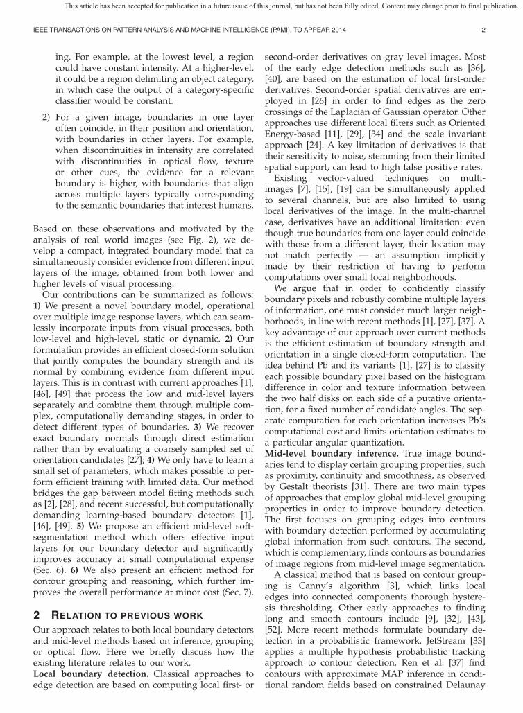
As shown in Fig. 3, ε controls the steepness ofthe boundary, going from completely planar when εis large to a sharp step-wise discontinuity throughthe window center p0, as ε approaches zero. Whenε is very small we have a step along the normalthrough the window center, and a sigmoid, along theboundary normal, that flattens as we move fartheraway from the center. As ε increases, the modelflattens to become a perfect plane for any ε greaterthan the window radius. In 2D, our model is not anideal ramp (see Fig. 3), a property which enables itto handle corners as well as edges. The idea of rampedges has been explored in the literature before, albeitvery differently [35]. Fig. 2 illustrates how boundaries

1. The output of a multi-label classifier can be encoded as mul-tiple input layers, where each layer represents a given label.

Fig. 3. Top: 1D view of our boundary model. Middle:2D view of the model with different values of ε relativeto the window radius R: 2a) ε > R ; 2b) ε = R/2 ;2c) ε = R/1000. For small ε the boundary model isa step along the normal passing through the windowcenter. Bottom: the model, for one layer, viewed fromabove: 3a) ε = R/2 ; 3b) ε = R/1000. The values onthe path [p, π(p), B, C] are the same. Inside the circlethe model is planar and outside is radially constant. Forsmall ε the radial line value ([p0, C]) varies linearly withthe cosine between that line and the boundary normal.

found by our proposed model correspond to thosevisible in real-world images and video.

When the window is far from any boundary, thevalue of bk should be near zero, since the only vari-ation in the layer values is due to noise. When weare close to a boundary, bk becomes large. The term(πε(p) − p0)

�n(p0) approximates the sign indicatingthe side of the boundary: it does not matter on whichside we are, as long as a sign change occurs when theboundary is crossed. When a true boundary is presentacross several layers at the same position (bk(p0) isnon-zero and possibly different, for several k) thenormal to the boundary should be consistent. Thus,we model the boundary normal n as common, andconstrained by all layers.

4 A CLOSED-FORM SOLUTION

We can now write the above equation in matrix formfor all layers, with the same window size and locationas follows: let X be a NW × K matrix with a row ifor each location pi of the window and a column for



each layer k, such that Xi;k = Lk(pi). Similarly, wedefine NW × 2 position matrix P: on its i-th row westore the x and y components of πε(pi)−p0 for the i-thpoint of the window. Let n = [nx, ny] be the boundarynormal and b = [b1, b2, . . . , bK ] the step sizes for layers1, 2, . . . ,K. Also, let us define the (rank-1) 2×K matrixJ = n�b. We also define matrix C of the same size asX, with each column k constant and equal to Ck(p0).We rewrite Eq. 1, with unknowns J and C (we dropp0 to simplify notation):

X ≈ C+PJ. (2)

Since C is a matrix with constant columns, and eachcolumn of P sums to 0, we have P�C = 0. Thus,by multiplying both sides of the above equation byP�, we eliminate the unknown C. Moreover, it can beeasily shown that P�P = αI, i.e., the identity matrixscaled by a factor α, which can be computed since Pis known. Thus, we obtain a simple expression for theunknown J (since both P and X are known):

J ≈ 1

αP�X. (3)

Since J = n�b, it follows that the matrix JJ� =‖b‖2n�

n is symmetric and has rank 1. Then n canbe estimated, in the least-squares sense, in terms ofthe principal eigenvector of M = JJ� and ‖b‖, asthe square root of its largest eigenvalue. ‖b‖ is thenorm of the boundary step vector b = [b1, b2, . . . , bK ]and captures the overall strength of boundaries fromall layers simultaneously. If the layers are properlyscaled, then ‖b‖ can be used as a measure of boundarystrength. Once we identify ‖b‖, we pass it through a1D logistic model to obtain the probability of bound-ary, similar to recent methods [1], [27]. The parametersof the logistic model are learned using standard proce-dures, detailed in Sec. 5.3. The normal to the boundaryn is then used for non-maximal suppression. Note that‖b‖ is different from the gradient of multi-images [7],[15] or the single channel method of [30], which usesecond-moment matrices computed from local deriva-tives. In contrast, we compute the boundary by fittinga model, which, by controlling the window size andε, ranges from planar to step-wise and accumulatesinformation over a small or large patch.Boundary strength along a given orientation. Insome cases we might want to compute the boundaryalong a given orientation n (e.g., when the true normalis known a priori, or if needed for a specific task).One way to do it is to start from the observationJJ� = ‖b‖2n�

n and estimate ‖b‖2 as the mini-mizer q∗ of the Frobenius norm ‖JJ� − qn�n‖F .It is relatively easy to show that the optimal q∗ isvec(JJ�)�vec(n�n) 1

‖n�n‖F. Both JJ� and n�n are

symmetric positive semidefinite, so their Frobeniusinner product vec(JJ�)�vec(n�n) = Tr(JJ�n�n)is nonnegative. This follows from the property thatthe product of positive semidefinite matrices is also

Fig. 4. Evaluation on the BSDS300 test set by varyingthe window size (in pixels), σG of the Gaussian weight-ing (relative to window radius) and ε. One parameteris varied, while the others are set to their optimum,learned from training images. Left: windows with largespatial support give a significantly better accuracy.Middle: points closer to the boundary should contributemore to the model, as evidenced by the best σG ≈half of the window radius. Right: small ε leads to betterperformance, validating our step-wise model.

positive semidefinite and the trace of a matrix is equalto the sum of its eigenvalues. Thus, the optimal q∗

is nonnegative and we can estimate ‖b‖ ≈ √q∗. The

solution for q∗ as a simple dot-product between two4-element vectors provides a very fast procedure toestimate the boundary strength along any orientation,once matrix M = JJ� is computed. This result, aswell as the proposed closed-form solution, are madepossible by our novel boundary model. In practice,computing the response of Gb over 8 quantized ori-entations is almost as fast as obtaining Gb based onthe closed-form solution and has similar performancein terms of the F-measure. Our contour reasoning(Section 7) is also robust and performs equally wellwith quantized orientations.Gaussian weighting. We propose to weigh each pixelin a window by an isotropic 2D Gaussian locatedat the window center p0. Such a spatially weightingplaces greater importance on fitting the model topoints closer to the window center.

The generalized boundary model is based on Eq. 2.The Gaussian weighting is applied such that theequation still holds, by multiplying each row of thematrices X, C, and P by the Gaussian weight appliedto the corresponding location within the window.This is equivalent to multiplying each side of Eq. 2with a diagonal matrix G, having diagonal elementsGii = g(xi−x0, yi−y0), where g is the Gaussian weightapplied at location pi = (xi, yi) relative to the windowcenter p0 = (x0, y0). We can re-write the equation as:

GX = GC+GPJ. (4)

The least squares solution for J in the above overde-termined system of equations is given by (to simplifynotation, we denote A = GP):

J = (A�A)−1A�GX− (A�A)−1A�GC. (5)

We observe that (A�A)−1 = ((GP)�GP)−1 is theidentity matrix multiplied by some scalar 1/α, and



that (GP)�GC = (G2P)�C = 0, since G = G�, ma-trix C has constant columns, and the columns ofmatrix G2P sum to 0. It follows that

J ≈ 1

α(GP)

�GX. (6)

Setting X ← GX and P ← GP, we obtain the sameexpression for J as in Eq. 3, which can also be writtenas J ≈ 1

α (G2P)

�X. To simplify notation, for the rest

of the paper, we set X ← GX and P ← GP, and useX and P, instead of GX and GP, respectively.

As seen in Fig. 4, the performance is influenced bythe choice of Gaussian standard deviation σG, whichsupports our prior belief that points closer to theboundary should have greater influence on the modelparameters. In our experiments we used a windowradius equal to 2% of the image diagonal, ε = 1 pixel,and Gaussian σG equal to half of the window radius.These parameters produced the best F-measure on theBSDS300 training set [27] and were also near-optimalon the test set, as shown in Fig. 4. From these experi-ments, we draw the following conclusions regardingthe proposed model: 1) A large window size leadsto significantly better performance as more evidencecan be integrated in reasoning about boundaries. Notethat when the window size is small our model isrelated to methods based on local approximation ofderivatives [3], [7], [15], [19]. 2) The usage of a small εproduces boundaries with significantly better localiza-tion and strength. It strongly suggests that perceptualboundary transitions in natural images tend to besudden, rather than gradual. 3) The center-weightingis justified: the model is better fitted if more weightis placed on points closer to the putative boundary.

5 ALGORITHM

Before applying the main algorithm we scale eachlayer in L according to its importance, which maybe problem dependent. We learn the scaling of layersfrom training data using a direct search method [20]to optimize the F-measure (Sec. 5.3). Alg. 1 (Gb)summarizes the proposed approach.

Algorithm 1 Gb: Generalized Boundary DetectionInitialize L, with each layer scaled appropriately.Initialize w0 and w1.Pre-compute matrix Pfor all pixels p doM ← (P

�Xp)(P

�Xp)

�

(v, λ) ← principal eigenpair of Mbp ← 1

1+exp(w0+w1

√λ)

θp ← atan2(vy, vx)end forreturn b, θ

The pseudo-code presented in Alg. 1 gives a de-scription of Gb that directly relates to our boundary

model. Upon closer inspection we observe that ele-ments of M can also be computed exactly by convo-lution, as explained next. X contains values from theinput layers, restricted to a particular window, andmatrix J is computed for each window location. UsingEq. 6 and observing that matrix G2P does not dependon the window center p0 = (x0, y0), the elements ofJ can be computed, for all window locations in theimage, by convolving each layer Lk twice, using twofilters: Hx(x−x0, y−y0) ∝ g(x−x0, y−y0)

2(xε−x0) andHy(x− x0, y− y0) ∝ g(x− x0, y− y0)

2(yε − y0), where(x, y) is p and (xε, yε) is πε(p). Specifically, Jp0(k, 1) =(Lk ∗ Hx)(x0, y0) and Jp0(k, 2) = (Lk ∗ Hy)(x0, y0).Then M = JJ� can be immediately obtained, for anygiven p0. These observations result in an easy-to-code,filtering-based implementation of Gb.2

5.1 Relation to Filtering-based Edge Detection

There is an interesting connection between the filtersused in Gb (e.g., Hx ∝ g(x−x0, y− y0)

2(xε−x0)) andGaussian Derivative (GD) filters (i.e., Gx(x − x0, y −y0) ∝ g(x−x0, y−y0)(x−x0)), which could be used forcomputing the gradient of multi-images [7]. Since thesquared Gaussian g(x − x0, y − y0)

2 from H is alsoGaussian, the main analytic difference between thetwo filters lies in our introduction of the projectionfunction πε(p). For an ε that is at least as large as thewindow radius, the two filters are the same, whichmeans that edge detection with Gaussian Derivativesis equivalent to fitting a linear (planar in 2D) edgemodel (Fig. 3) with Gaussian weighted least-squares.From this point of view Gb filters could be seen as ageneralization of Gaussian Derivatives.

Fig. 5 presents the Gb and GD filters from twodifferent view-points. Gaussian derivatives have thecomputational advantage of being separable. On theother hand, Gb filters with small ε are better suitedfor real world, perceptual boundaries (see Fig. 2):they are steep perpendicular to the boundary, witha pointed shape along the boundary. This allows abetter handling of corners, as seen in the examplegiven in Fig. 5, bottom row. In practice, small ε givessignificantly better results over large ε, both qualita-tively and quantitatively: on BSDS300 the F-measuredrops by about 1.5% when ε = window radius is used,with all other parameters being optimized (Fig. 4).

Our approach differs from traditional filteringbased edge detectors [18] in the following ways: 1)Gb filters not only the image but also other layers ofthe image, resulting from different visual processes,low-level or high-level, static or dynamic, such as soft-segmentation or optical flow; 2)Gb boundaries are notcomputed directly from filter responses, but only after

2. Code available at: http://www.imar.ro/clvp/code/Gb,as well as sites.google.com/site/gbdetector/, andhttp://www.maths.lth.se/matematiklth/personal/sminchis/code/index.html.



Fig. 5. A. Gb filters. B. Gaussian Derivative (GD)filters C. Output (zoomed in) of Gb and GD (after non-maximal suppression) for a dark line (5 pixels thin),having identical parameters (except for ε) and windowsize = 19 pixels. GD has poorer localization and cornerhandling. Note: asymmetry in GD output is due tonumerical issues in the non-maximal suppression.

building matrix M = JJ� and computing its principaleigenpair (Alg. 1). Gb provides a potentially revealingconnection between model fitting and filtering-basededge detection.

5.2 Computational ComplexityThe overall complexity of Gb is straightforward toderive. For each pixel p, the most expensive step iscomputing the matrix M, which has O((NW + 2)K)complexity, where NW denotes the number of pixelsin the window and K is the number of layers. M isa 2 × 2 matrix, so computing its eigenpair (v, λ) isa closed-form operation, with small fixed cost. Thus,for a fixed NW and a total of N pixels per image theoverall complexity is O(KNWN). If NW is a fractionf of N , then complexity becomes O(fKN2).

The running time of Gb compares favorably to thatof Pb [1], [27]. Pb in its exact form has complexityO(fKNoN

2), where No is a discrete number of can-didate orientations. Both Gb and Pb are quadraticin the number of image pixels. However, Pb has asignificantly larger fixed cost per pixel as it requiresthe computation of histograms for each individualimage channel and for each orientation. In Fig. 6, weshow the run times for Gb and Pb (based on publiclyavailable code) on a 3.2 GHz desktop. These are MAT-LAB implementations, run on the same images, usingthe same window size and a single scale. While Gbproduces boundaries of similar quality (see Table 2),it is consistently 1–2 orders of magnitude faster thanPb (about 40×), independent of the image size (Fig. 6,

TABLE 1Run times: Gb in MATLAB (without using mex files) on

a 3.2 GHz desktop vs. Catanzaro et al.’s parallelcomputation of local cues on Nvidia GTX 280 [5].

Algorithm Gb (exact) [5] (exact) [5] (approx.)

Run time (sec.) 0.473 4.0 0.569

right). For example, on 0.15 MP images the times are:19.4 sec. for Pb vs. 0.48 sec. for Gb; to process 2.5 MPimages, Pb takes 38 min while Gb only 57 sec.

A parallellized implementation of gPb is proposedin [5], where method is implemented directly on ahigh-performance Nvidia GTX 280 graphics card with240 CUDA cores. Local Pb is computed at three dif-ferent scales. The authors offer two implementationsfor local cues: one for the exact computation and theother for a faster approximate computation that usesintegral images and is linear in the number of imagepixels. The approximation has O(fKNoNbN) timecomplexity, where Nb is the number of histogram binsfor different image channels and No is the numberof candidate orientations. Note that NoNb is large inpractice and affects the overall running time consid-erably. It requires computing (and possibly storing) alarge number of integral images, one for each combi-nation of (histogram bin, image channel, orientation).The actual number is not explicitly stated in [5], butwe estimate that it is in the order of 1000 per inputimage (4 channels × 8 orientations × 32 histogrambins = 1024). The approximation also requires specialprocessing of the rotated integral images of textonlabels, to minimize interpolation artifacts. The authorspropose a solution based on Bresenham lines, whichmay also, to some degree impact the discretizationof the rotation angle. In Table 1 we present run timecomparisons with Pb’s local cues computation from[5]. Our exact implementation of Gb (using 3 colorlayers) in MATLAB is 8 times faster than the exactparallel computation of Pb over 3 scales on GTX 280.

5.3 Learning

Our model uses a small number of parameters. Onlytwo parameters (w0, w1) are needed for the logisticfunction that models the probability of boundary(Alg. 1). The role of these parameters is to strengthenor weaken the output, but they do not affect thequantitative performance since the logistic functionis monotonically increasing in the eigenvalue of M,λ. Instead, the parameters only affect the F-measurefor a fixed, desired threshold. For layer scaling themaximum number of parameters needed is equal tothe number of layers. We reduce this number by tyingthe scaling for layers of the same type: 1) for color (inCIELAB space) we fix the scale of L to 1 and learn a



Fig. 6. Left: Edge detection run times on a 3.2 GHzdesktop for our MATLAB-only implementation of Gb vs.the publicly available code of Pb [27]. Right: ratio of runtime of Pb to run time of Gb, experimentally confirmingthat Pb and Gb have the same time complexity, but Gbhas a significantly lower fixed cost per iteration. Eachalgorithm runs over a single scale and uses the samewindow size, which is a constant fraction of the imagesize. Here, Gb is 40× faster.

single scaling for both channels a and b; 2) for soft-segmentation (Sec. 6) we learn a single scaling for all8 segmentation layers; 3) for optical flow (Sec. 8.2) welearn one parameter for the 2 flow channels, anotherfor the 2 channels of the unit normalized flow, and athird for the flow magnitude.

Learning layer scaling is based on the observationthat M is as a linear combination of matrices Mi

computed separately for each layer scaling si:

M =∑i

s2iMi, (7)

where Mi ← (P�Xi)(P�Xi)

� and Xi is the subma-trix of X, with the same number of rows as X andwith columns corresponding only to those layers thatare scaled by si. It follows that the largest eigenvalueof M, λ = 1

2 (Tr(M) +√

Tr(M)2 − det(M)/4), can becomputed from si’s and the elements of Mi’s. Thus,the F-measure, which depends on (w0, w1) and λ,can also be computed over the training data as afunction of the parameters (w0, w1) and si, whichhave to be learned. To optimize the F-measure, weuse the direct search method of Lagarias et al. [20],since it does not require an analytic form of the costand can be easily implemented in MATLAB by usingthe fminsearch function. In our experiments, thepositive and negative training edges were sampledat equally spaced locations on the output of Gb usingonly color, with all channels equally scaled (after non-maximal suppression applied directly on the raw

√λ).

Positive samples are the ones sufficiently close (< 3pixels) to the human-labeled ground truth boundaries.

6 EFFICIENT SOFT-SEGMENTATION

In this section we present a novel method to rapidlygenerate soft image segmentations. Its continuousoutput is similar to the Ncuts eigenvectors [44], butits computational cost is significantly lower: about

2.5 sec. (3.2 GHz CPU) vs. over 150 sec. requiredfor Ncuts (2.66 GHz CPU [5]) per 0.15 MP image inMATLAB (no mex files). We briefly describe it herebecause it serves as a fast mid-level representation ofthe image that significantly improves the boundarydetection accuracy over raw color alone.

We assume that the color of any image pixel has acertain probability of occurrence, given the semanticregion (e.g., object) to which it belongs -the image isformed by a composition of semantic regions withdistinct color distributions, which are location inde-pendent given the region. Thus, colors of any imagepatch are generated from a certain, patch-dependent,linear combination (mixture) of these finite numberof distributions: if the patch is from a single regionthen it will have a single generating distribution; if thepatch is in between regions then it will be generatedfrom a mixture of distributions depending on thepatch location relative to those regions. Let c be anindicator vector of some image patch, such that cj = 1if color j is present in the patch and 0 otherwise. Thenc is a multi-dimensional Bernoulli random variabledrawn from its mixture: c ∼ ∑

i πi(c)hi.Based on this model, the space of all c’s from

a given image will contain redundant information,reflecting the regularity of real-world scenes throughthe underlying generative distributions. We discoverthe linear subspace of these distributions, that is itseigendistributions vi’s, by applying PCA to a suffi-ciently large set of indicator vectors c sampled uni-formly from the image. Then, for any given patch,the generating foreground distribution of its associatedindicator vector c could be approximated by means ofPCA reconstruction: hF(c) ≈ h0 +

∑i((c− h0)

�vi)vi.Here h0 is the sample mean, the overall empiricalcolor distribution of the whole image.

We consider the background distribution to be onethat is as far as possible (in the subspace) from theforeground, by using the same coefficients but withopposite sign: hB(c) ≈ h0 −

∑i((c− h0)

�vi)vi. ThenhF(c) and hB(c) are used to obtain the foreground (F)posterior probability for each image pixel i, based onits color xi, by applying Bayes’ rule with equal priors:

P (c)(F|xi) =h(c)F (xi)

h(c)F (xi) + h

(c)B (xi)

≈ h(c)F (xi)

2h0. (8)

Given an image patch, we quickly obtain a pos-terior probability of foreground (F) for each imagepixel, resulting in a soft figure/ground segmentation(Fig. 9). These figure/ground segmentations are sim-ilar in spirit to the segmentation hints based on alphamatting [23], used by Stein et al. [47] for full objectsegmentation. The figure/ground segmentations areoften redundant when different patches are centeredat different locations on the same object–a direct resultof the first stage, when a reduced subspace for colordistributions is learned. Thus, many of such soft



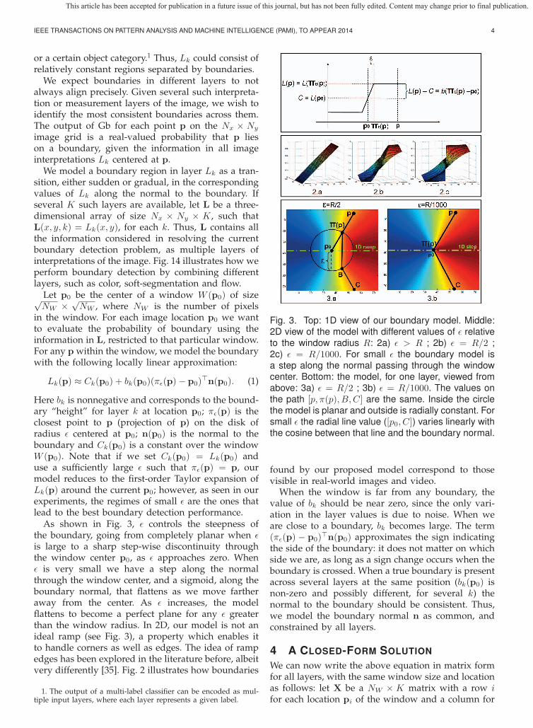
Fig. 7. Soft-segmentation results from our method. The first 3 dimensions of the soft-segmentations are shownon the RGB channels. Computation time for soft-segmentation is ≈2.5 seconds per 0.15 MP image in MATLAB.

figure/ground probability maps can be compressedto obtain a few representative soft figure/groundsegmentations of the same image, as detailed next.

We perform the same classification procedure for ns

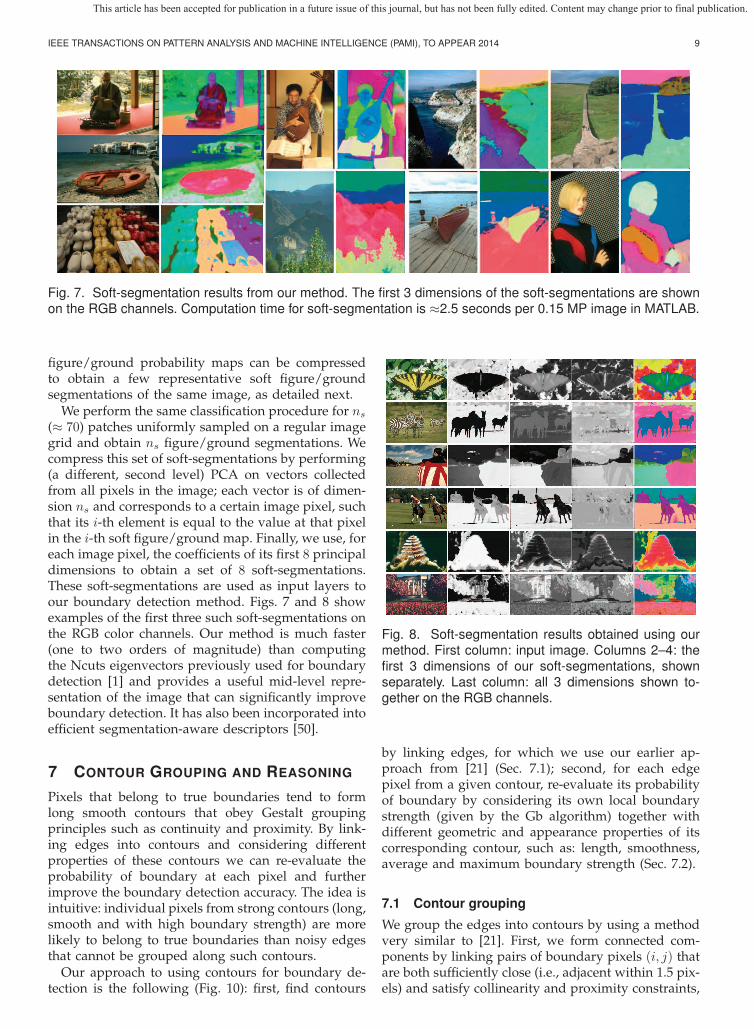
(≈ 70) patches uniformly sampled on a regular imagegrid and obtain ns figure/ground segmentations. Wecompress this set of soft-segmentations by performing(a different, second level) PCA on vectors collectedfrom all pixels in the image; each vector is of dimen-sion ns and corresponds to a certain image pixel, suchthat its i-th element is equal to the value at that pixelin the i-th soft figure/ground map. Finally, we use, foreach image pixel, the coefficients of its first 8 principaldimensions to obtain a set of 8 soft-segmentations.These soft-segmentations are used as input layers toour boundary detection method. Figs. 7 and 8 showexamples of the first three such soft-segmentations onthe RGB color channels. Our method is much faster(one to two orders of magnitude) than computingthe Ncuts eigenvectors previously used for boundarydetection [1] and provides a useful mid-level repre-sentation of the image that can significantly improveboundary detection. It has also been incorporated intoefficient segmentation-aware descriptors [50].

7 CONTOUR GROUPING AND REASONING

Pixels that belong to true boundaries tend to formlong smooth contours that obey Gestalt groupingprinciples such as continuity and proximity. By link-ing edges into contours and considering differentproperties of these contours we can re-evaluate theprobability of boundary at each pixel and furtherimprove the boundary detection accuracy. The idea isintuitive: individual pixels from strong contours (long,smooth and with high boundary strength) are morelikely to belong to true boundaries than noisy edgesthat cannot be grouped along such contours.

Our approach to using contours for boundary de-tection is the following (Fig. 10): first, find contours

Fig. 8. Soft-segmentation results obtained using ourmethod. First column: input image. Columns 2–4: thefirst 3 dimensions of our soft-segmentations, shownseparately. Last column: all 3 dimensions shown to-gether on the RGB channels.

by linking edges, for which we use our earlier ap-proach from [21] (Sec. 7.1); second, for each edgepixel from a given contour, re-evaluate its probabilityof boundary by considering its own local boundarystrength (given by the Gb algorithm) together withdifferent geometric and appearance properties of itscorresponding contour, such as: length, smoothness,average and maximum boundary strength (Sec. 7.2).

7.1 Contour grouping

We group the edges into contours by using a methodvery similar to [21]. First, we form connected com-ponents by linking pairs of boundary pixels (i, j) thatare both sufficiently close (i.e., adjacent within 1.5 pix-els) and satisfy collinearity and proximity constraints,



Fig. 9. Examples of soft figure/ground segmentationsbased on the current patch, shown in red. Note thatthe figure/ground soft-segmentations are similar forpatches centered on different locations of the sameobject; this justifies our final PCA compression.

ensuring that the components only contain smoothcontours. For each connected component c we form itsweighted adjacency matrix A such that Aij is positiveif edge pixels (i, j) are connected and 0 otherwise:

Aij =

{1− θ2

ij

σ2θ

if (i, j) are neighbors and θij < σθ

0 otherwise,

where θij ≥ 0 is the smallest (positive) angle betweenthe boundary normals at pixels i and j and σθ isa predefined threshold. The value of Aij increaseswith the similarity between the boundary normals atneighboring pixels. Therefore, smooth contours havelarger average values in their adjacency matrix A.

Let p be the current pixel and c(p) the label ofits contour. The following two geometric cues arecomputed for each contour (used by the contour-based boundary classification method, explained inSection 7.2): 1). the contour length, computed as thenumber of pixels of component c(p) normalized by thelength of the image diagonal; 2). the average contoursmoothness estimated as the sum of elements in Ac(p)

divided by the length of c(p).

7.2 Contour reasoning

Our classification scheme has two stages, with a struc-ture similar to a two-layer neural network, havinglogistic linear classifiers at all nodes, both hidden andfinal output (Figure 10). The main difference is in thetraining and its design: each node and connection ischosen manually and training is performed sequen-tially, bottom-up, from the first level to the last.

At the first level in the hierarchy, we first train ageometry-only logistc boundary classifier Cgeom (usingstandard linear logistic regression) applied to each

Fig. 10. Overview of the contour reasoning framework.First, an edge map is obtained from the input imageusing a Gb model with color and soft segmentationlayers. Then edges are linked to form contours. Next,using two logistic classifiers we label the edge pixelsbased on different properties of their contours: ap-pearance (boundary strength) or geometry (length andsmoothness). The outputs of these two classifiers arethen combined to obtain the final boundary map.

contour pixel using two features: the length and av-erage smoothness of the contour fragment (computedas explained in Sec. 7.1). Second, also at the first level,we train an appearance-only logistic edge classifier Capp(again applied to each contour pixel, trained by linearlogistic regression) using the following three cues:local boundary strength at the current pixel, averageand maximum boundary strength over the contour.The soft outputs of these two classifiers become in-puts to the final linear logistic boundary classifier,at the second level in the hierarchy, which is alsotrained using logistic regression. The separate trainingof each classifier is performed due to its efficiency,but more sophisticated learning methods could alsobe employed for fine-tuning parameters. The frame-work (Fig. 10) is related to late fusion schemes fromsemantic video analysis and indexing [45], [53], inwhich separate independent classifiers are trainedand their outputs are then combined using a second-level classifier. The steps of our contour grouping andreasoning algorithm are:

1) Run the Gb method described in Alg. 1 with nonlocal maximal suppression to obtain thin edges.



Fig. 11. Top row: input images from BSDS300 dataset.Second row: output of a Gb model that uses onlycolor layers. Third row: output of a Gb model that usesboth color and soft-segmentation. Bottom row: outputof a more complex Gb model that leverages color, softsegmentation and contour reasoning.

2) Remove the edge pixels with low boundarystrength.

3) Group the surviving edges into contours usingthe method from Sec. 7.1.

4) For each contour pixel compute the probabilityof boundary using the geometry-only logistic clas-sifier Cgeom.

5) For each contour pixel compute the probabilityof boundary using the appearance-only logisticclassifier Capp.

6) For each contour pixel compute the final proba-bility of boundary with a logistic classifier thatcombines the outputs of Cgeom and Capp.

8 EXPERIMENTS

To evaluate the generality of our proposed method,we conduct experiments on detecting boundaries inboth images and video. First, we show results on staticimages. Second, we perform experiments on occlusionboundary detection in short video clips.

8.1 Boundaries in Static Color Images

We evaluate Gb on the well-known BSDS300dataset [27] (Fig. 11). We compare the accuracy andcomputational time of Gb with other published meth-ods (see Table 2). For Gb we present results us-ing color (C), color and soft-segmentation (C+S),and color, soft-segmentation and contour grouping(C+S+G). We also include results on gray-scale im-ages. The total times reported for Gb include allprocessing needed (MATLAB-only, without compiledmex files): for example, for Gb(C+S+G) the reported

Fig. 12. Qualitative boundary detection results forimages from BSDS300 (first row), obtained with a Gbmodel that uses only color layers (second row), Pb(third row), GD (fourth row), and Canny (last row).

times include computing soft-segmentations, bound-ary detection (Alg. 1) and contour reasoning. Gbachieves a competitive F-measure of 0.69 very fast,compared to current state of the art techniques. Forexample, the method of [37] obtains an F-measureof 0.68 on this dataset by combining the output ofPb at three scales. Note that the same multi-scalemethod could use Gb instead, which can potentiallyimprove the overall performance of our approach.Global Pb [1], [5] achieves an F-measure of 0.70 byusing the significantly more expensive Ncuts soft-segmentations. Note that our formulation is generaland could incorporate other segmentations (such asNcuts, CPMC [4], or compositional methods [14]).

Our proposed Gb is competitive even when usingonly color layers alone at a processing speed of 0.5 sec.per image in pure Matlab. In Fig. 12 we present afew comparative results of four different local, singlescale boundary detectors: Gb using only color, Pb [27],Gaussian derivatives (GD) for the gradient of multi-images [19], and Canny [3] edge detectors (Table 2).Canny uses brightness information, Gb and GD usebrightness and color and Pb uses brightness, color andtexture. Gb, Pb and GD use the same window size.The benefit from soft-segmentation: In Fig. 13 wepresent the output of Gb using only the first 3 di-



Fig. 13. Boundary detection examples, obtained usinga Gb model that uses only the first 3 dimensions of oursoft-segmentations as input layers. Note: color layerswere not used here.

mensions of our soft-segmentations as input layers(no color information was used). We came to thefollowing conclusions: 1) while soft-segmentations donot separate the image into disjoint regions (as hard-segmentation does), their boundaries are correlatedespecially with occlusions and whole object bound-aries (as also confirmed by our results on CMUMotion Dataset [46]); 2) soft-segmentations cannotcapture the fine details of objects or texture, but, incombination with raw color layers, they can signifi-cantly improve Gb’s performance on detecting generalboundaries in static natural images.

Fig. 14. Output of a Gb model using color and soft seg-mentation layers, without contours (second column)and with contours (third column) after thresholdingat the optimal F-measure. The use of global contourreasoning produces a cleaner output.

The benefit from contour reasoning: Besides the

TABLE 2Comparison of F-measure and total runtime in

MATLAB. For Gb (C+S+G) it includes the computationof soft-segmentations (S) and contour reasoning (G).

Algorithm F-measure Total run time (sec.)

Gb (C+S+G) 0.69 6.0Gb (C+S) 0.67 5.5Gb (C) 0.65 0.5Gb (graylevel+G) 0.63 0.2Gb (graylevel) 0.61 0.15SCG Ren and Bo [38] 0.715 > 175gPb - Arbelaez et al. [1] 0.70 175Multiscale - Ren [37] 0.68 60Mairal et al. [25] 0.66 NABEL - Dollar et al. [8] 0.66 NAFelzenszwalb et al. [10] 0.65 NACRF - Ren et al. [39] 0.64 NAPb - Martin et al. [27] 0.65 20GD (C) [19] 0.62 0.3GD (graylevel) [19] 0.58 0.1Canny (graylevel) [3] 0.58 0.1

solid improvement of 2% in F-measure over Gb(C+S)and Gb (graylevel), the contour reasoning module(denoted by G in Table 2), which runs in less than0.5 sec. in MATLAB per 0.15 MP image, brings thefollowing qualitative advantage (see also Fig. 14): dur-ing this last stage, edge pixels belonging to the samecontour tend to end up with very similar probabilitiesof boundaries. This outcome is intuitive, since pixelsbelonging to one contour should either be acceptedor rejected together. Thus, for any given decisionthreshold, the surviving edge map will look clean,with very few isolated edge pixels. The qualitative im-provement after contour reasoning is visually strikingafter cutting by the optimal threshold (see Fig. 14).

To test our model’s robustness to overfitting weperformed 30 different learning experiments for Gb(C+S) using 30 images randomly sampled from theBSDS300 training set. As a result, we obtained thesame F-measure on the 100 images test set (measuredσ < 0.1%), confirming that the representation and theparameter learning procedure are robust.

In Fig. 12 we present some additional examplesof boundary detection. We show boundaries detectedwith Gb(C), Pb [27], GD and the Canny edge de-tector [3]. Both Gb and GD use only color layers,identically scaled, with the same window size andGaussian weighting. GD is based on the gradient ofmulti-images [19], which we computed using Deriva-tive of Gaussian filters. While in classical work onedge detection from multi-images [7], [19] the channelgradients are computed over small image neighbor-hoods, in our paper we use Derivative of Gaussianfilters of the same size as the window applied toGb, for a fair comparison. Note that Pb uses colorand texture, while Canny is based only on brightnesswith derivatives computed at a fine scale. For Cannywe used the MATLAB function edge with thresholds[0.1, 0.25]. Run-times in MATLAB-only per image, for



Fig. 15. Gb results on the CMU Motion Dataset.

each method, are: Gb - 0.5 sec., Pb - 19.4 sec., GD -0.3 sec., and Canny - 0.1 sec.

These examples confirm, once again, that: 1) Gbmodels that use only color layers produce boundariesthat are of similar quality as Pb’s; 2) methods basedon local derivatives, such as Canny, cannot producehigh quality boundaries on difficult, highly-textured,color images; and 3) using Gaussian Derivativeswith a large standard deviation could remove noisyedges (reduce false positives) and improve boundarystrength, but at the cost of poorer localization anddetection (increases the false negative rate). Note thatGaussian smoothing suppresses the high-frequencies,which are important for boundary detection. In con-trast, our generalized boundary model, with a regimeof small ε, is more sensitive in localization and cor-rectly captures the general notion of boundaries assudden transitions among different image regions.

8.2 Occlusion Boundaries in VideoMultiple video frames, closely spaced in time, providesignificantly more information about dynamic scenesand make occlusion boundary detection possible, asshown in recent work [13], [42], [46], [49]. State ofthe art techniques for occlusion boundary detectionin video are based on combining, in various ways,the outputs of existing boundary detectors for staticcolor images with optical flow, followed by a globalprocessing phase [13], [42], [46], [49]. Table 3 com-pares Gb against reported results on the CMU MotionDataset [46] We use, as one of our layers, the flowcomputed using Sun et al.’s public code [48]. Addi-tionally, Gb uses color and soft segmentation (Sec. 6),as described in the previous sections. In contrast toother methods [13], [42], [46], [49], which require sig-nificant time for processing and optimization, we re-quire less than 1.6 sec. on average to process 230×320images from the CMU dataset (excluding Sun et al.’sflow computation). Fig. 15 shows qualitative results.

9 CONCLUSIONS

We have presented Gb, a novel model and algorithmfor generalized boundary detection. Gb effectivelycombines multiple low- and mid-level interpretationlayers of an image in a principled manner, and

TABLE 3Occlusion boundary detection, using a Gb model with

optical flow layer, on the CMU Motion Dataset.

Algorithm F-measure

Gb 0.62Sundberg et al. [49] 0.61He & Yuille [13] 0.47Sargin et al. [42] 0.57Stein et al. [46] 0.48

resolves their constraints jointly, in closed-form, inorder to compute the exact boundary strength andorientation. Consequently, Gb achieves state of the artresults on published datasets at a significantly lowercomputational cost than current methods. For mid-level inference, we present two efficient methods forsoft-segmentation, and contour grouping and reason-ing, which significantly improve the boundary de-tection performance at negligible computational cost.Gb’s broad real-world applicability is demonstratedthrough quantitative and qualitative results on thedetection of boundaries in natural images and theidentification of occlusion boundaries in video.

ACKNOWLEDGMENTS

The authors would like to thank Andrei Zanfir forhelping with parts of the code. This work was sup-ported in part by CNCS-UEFICSDI, under PNII RU-RC-2/2009, PCE-2011-3-0438, PCE-2012-4-0581, andCT-ERC-2012-1.

REFERENCES[1] P. Arbelaez, M. Maire, C. Fowlkes, and J. Malik. Contour

detection and hierarchical image segmentation. PAMI, 33(5),2011.

[2] S. Baker, S. K. Nayar, and H. Murase. Parametric featuredetection. In DARPA IUW, 1997.

[3] J. Canny. A computational approach to edge detection. PAMI,8(6), 1986.

[4] J. Carreira and C. Sminchisescu. CPMC: Automatic objectsegmentation using constrained parametric min-cuts. PAMI,34(7), 2012.

[5] B. Catanzaro, B.-Y. Su, N. Sundaram, Y. Lee, M. Murphy, andK. Keutzer. Efficient, high-quality image contour detection. InICCV, 2009.

[6] A. Cumani. Edge detection in multispectral images. CVGIP,53(1), 1991.

[7] S. Di Senzo. A note on the gradient of a multi-image. CVGIP,33(1), 1986.

[8] P. Dollar, Z. Tu, and S. Belongie. Supervised learning of edgesand object boundaries. In CVPR, 2006.

[9] J. Elder and S. Zucker. Computing contour closures. In ECCV,1995.

[10] P. Felzenszwalb and D. McAllester. A min-cover approach forfinding salient curves. In CVPRW, 2006.

[11] W. T. Freeman and E. H. Adelson. The design and use ofsteerable filters. PAMI, 13(9), 1991.

[12] B. Hariharan, P. Arbelaez, L. Bourdev, S. Maji, and J. Malik.Semantic contours from inverse detectors. In ICCV, 2011.

[13] X. He and A. Yuille. Occlusion boundary detection usingpseudo-depth. In ECCV, 2010.

[14] A. Ion, J. Carreira, and C. Sminchisescu. Image segmentationby figure-ground composition into maximal cliques. In ICCV,2011.

[15] T. Kanade. Image understanding research at CMU. In DARPAIUW, 1987.



[16] I. Kokkinos. Boundary detection using f-measure, filter- andfeature-(f3) boost. In ECCV, 2010.

[17] I. Kokkinos. Highly accurate boundary detection and group-ing. In CVPR, 2010.

[18] S. Konishi, A. Yuille, and J. Coughlan. Fundamental boundson edge detection: An information theoretic evaluation ofdifferent edge cues. In CVPR, 1999.

[19] M. Koschan and M. Abidi. Detection and classification ofedges in color images. SPM-SICIP, 22(1), 2005.

[20] J. Lagarias, J. A. Reeds, M. H. Wright, and P. E. Wright.Convergence properties of the Nelder-Mead simplex methodin low dimensions. SIAM Optimization, 9(1), 1998.

[21] M. Leordeanu, M. Hebert, and R. Sukthankar. Beyond localappearance: Category recognition from pairwise interactionsof simple features. In CVPR, 2007.

[22] M. Leordeanu, R. Sukthankar, and C. Sminchisescu. Efficientclosed-form solution to generalized boundary detection. InECCV, 2012.

[23] A. Levin, D. Lischinski, and Y. Weiss. A closed form solutionto natural image matting. In CVPR, 2006.

[24] T. Lindeberg. Edge detection and ridge detection with auto-matic scale selection. IJCV, 30(2), 1998.

[25] J. Mairal, M. Leordeanu, F. Bach, M. Hebert, and J. Ponce.Discriminative sparse image models for class-specific edgedetection and image interpretation. In ECCV, 2008.

[26] D. Marr and E. Hildtreth. Theory of edge detection. In Proc.Royal Society, 1980.

[27] D. Martin, C. Fawlkes, and J. Malik. Learning to detect naturalimage boundaries using local brightness, color, and texturecues. PAMI, 26(5), 2004.

[28] P. Meer and B. Georgescu. Edge detection with embeddedconfidence. PAMI, 23(12), 2001.

[29] M. Morron and R. Owens. Detecting and localizing edgescomposed of steps, peaks and roofs. Pattern Recognition Letters,1987.

[30] M. Nitzberg and T. Shiota. Nonlinear image filtering with edgeand corner enhancement. PAMI, 14(8), 1992.

[31] S. Palmer. Vision science: photons to phenomenology. 1999.[32] P. Parent and S. Zucker. Trace inference, curvature consistency,

and curve detection. PAMI, 11(8), 1989.[33] P. Perez, A. Blake, and M. Gagnet. Jetstream: Probabilistic

contour extraction with particles. In ICCV, 2001.[34] P. Perona and J. Malik. Detecting and localizing edges com-

posed of steps, peaks and roofs. In ICCV, 1990.[35] M. Petrou and J. Kittler. Optimal edge detectors for ramp

edges. PAMI, 13(5), 1991.[36] J. Prewitt. Object enhancement and extraction. In Picture

Processing and Psychopictorics. Academic Press, 1970.[37] X. Ren. Multi-scale improves boundary detection in natural

images. In ECCV, 2008.[38] X. Ren and L. Bo. Discriminatively trained sparse code

gradients for contour detection. In NIPS, 2012.[39] X. Ren, C. Fowlkes, and J. Malik. Scale-invariant contour

completion using conditional random fields. In ICCV, 2005.[40] L. Roberts. Machine perception of three-dimensional solids.

In Optical and Electro-Optical Information Processing. 1965.[41] M. Ruzon and C. Tomasi. Edge, junction, and corner detection

using color distributions. PAMI, 23(11), 2001.[42] M. Sargin, L. Bertelli, B. Manjunath, and K. Rose. Probabilistic

occlusion boundary detection on spatio-temporal lattices. InICCV, 2009.

[43] A. Shashua and S. Ullman. Structural saliency: the detection ofglobally salient structures using a locally connected network.In ICCV, 1988.

[44] J. Shi and J. Malik. Normalized cuts and image segmentation.PAMI, 22(8), 2000.

[45] C. Snoek, M. Worring, and A. Smeulders. Early versus latefusion in semantic video analysis. In ACM-ICM, 2005.

[46] A. Stein and M. Hebert. Occlusion boundaries from motion:Low-level detection and mid-level reasoning. IJCV, 82(3), 2009.

[47] A. Stein, T. Stepleton, and M. Hebert. Towards unsupervisedwhole-object segmentation: Combining automated mattingwith boundary detection. In CVPR, 2008.

[48] D. Sun, S. Roth, and M. Black. Secrets of optical flowestimation and their principles. In CVPR, 2010.

[49] P. Sundberg, T. Brox, M. Maire, P. Arbelaez, and J. Malik.Occlusion boundary detection and figure/ground assignmentfrom optical flow. In CVPR, 2011.

[50] E. Trulls, I. Kokkinos, A. Sanfeliu, and F. Moreno-Noguer.Dense segmentation-aware descriptors. In CVPR, 2013.

[51] N. Widynski and M. Mignotte. A particle filter framework forcontour detection. In ECCV, 2012.

[52] L. Williams and D. Jacobs. Stochastics completion fields: Aneural model of illusory contour shape and salience. In ICCV,1995.

[53] G. Ye, D. Liu, I.-H. Jhuo, and S.-F. Chang. Robust late fusionwith rank minimization. In CVPR, 2012.

[54] Q. Zhu, G. Song, and J. Shi. Structural saliency: the detection ofglobally salient structures using a locally connected network.In ICCV, 1988.

Marius Leordeanu is a senior researchscientist at the Institute of Mathematics ofthe Romanian Academy. Marius receivedhis Ph.D. in Robotics from Carnegie MellonUniversity in 2009 and Bachelor degrees inMathematics and Computer Science fromthe City University of New York, 2003. Hisresearch focuses on computer vision andmachine learning, with contributions in learn-ing and optimization for matching and prob-abilistic graphical models, object category

recognition, object tracking, 3D modeling of urban scenes, videounderstanding and boundary detection.

Rahul Sukthankar is a scientist at GoogleResearch, an adjunct research professor inthe Robotics Institute at Carnegie Mellon andcourtesy faculty in EECS at the University ofCentral Florida. He was previously a seniorprincipal researcher at Intel Labs, a senior re-searcher at HP/Compaq Labs and researchscientist at Just Research. He received hisPh.D. in Robotics from Carnegie Mellon in1997 and his B.S.E. in Computer Sciencefrom Princeton in 1991. His current research

focuses on computer vision and machine learning, particularly inthe areas of object recognition, video understanding and informationretrieval.

Cristian Sminchisescu has obtained a doc-torate in Computer Science and AppliedMathematics with an emphasis on imaging,vision and robotics at INRIA, France, underan Eiffel excellence doctoral fellowship, andhas done postdoctoral research in the Artifi-cial Intelligence Laboratory at the Universityof Toronto. He is a member in the programcommittees of the main conferences in com-puter vision and machine learning (CVPR,ICCV, ECCV, NIPS, AISTATS), area chair for

ICCV07-13, and an Associate Editor of IEEE PAMI. He has givenmore than 100 invited talks and presentations and has offeredtutorials on 3d tracking,recognition and optimization at ICCV andCVPR, the Chicago Machine Learning Summer School, the AERFAIVision School in Barcelona and the Computer Vision Summer School(VSS) in Zurich. His research interests are in the area of computervision (3D human pose estimation, semantic segmentation) andmachine learning (optimization and sampling algorithms, structuredprediction, and kernel methods).


ieee transactions on pattern analysis and …rahuls/pub/gb-pami-rahuls.pdfof boundary detection...

Documents