IEEE TRANSACTIONS ON INFORMATION THEORY, VOL. .., NO. .., .. 1

Asymptotic Analysis of Complex LASSO viaComplex Approximate Message Passing (CAMP)

Arian Maleki, Laura Anitori, Zai Yang, and Richard Baraniuk, Fellow, IEEE

Abstract—Recovering a sparse signal from an undersampledset of random linear measurements is the main problem ofinterest in compressed sensing. In this paper, we consider thecase where both the signal and the measurements are complex-valued. We study the popular recovery method of `1-regularizedleast squares or LASSO. While several studies have shown thatLASSO provides desirable solutions under certain conditions, theprecise asymptotic performance of this algorithm in the complexsetting is not yet known. In this paper, we extend the approximatemessage passing (AMP) algorithm to solve the complex-valuedLASSO problem and obtain the complex approximate messagepassing algorithm (CAMP). We then generalize the state evolutionframework recently introduced for the analysis of AMP to thecomplex setting. Using the state evolution, we derive accurateformulas for the phase transition and noise sensitivity of bothLASSO and CAMP. Our theoretical results are concerned withthe case of i.i.d. Gaussian sensing matrices. Simulations confirmthat our results hold for a larger class of random matrices.

Index Terms—compressed sensing, complex-valued LASSO,approximate message passing, minimax analysis.

I. INTRODUCTION

Recovering a sparse signal from an undersampled set ofrandom linear measurements is the main problem of interestin compressed sensing (CS). In the past few years many algo-rithms have been proposed for signal recovery, and their per-formance has been analyzed both analytically and empirically[1]–[6]. However, whereas most of the theoretical work hasfocussed on the case of real-valued signals and measurements,in many applications, such as magnetic resonance imaging andradar, the signals are more easily representable in the complexdomain [7]–[10]. In such applications, the real and imaginarycomponents of a complex signal are often either zero ornon-zero simultaneously. Therefore, recovery algorithms maybenefit from this prior knowledge. Indeed the results presentedin this paper confirm this intuition.

Motivated by this observation, we investigate the perfor-mance of the complex-valued LASSO in the case of noise-free and noisy measurements. The derivations are based on thestate evolution (SE) framework, presented previously in [3].Also a new algorithm, complex approximate message passing(CAMP), is presented to solve the complex LASSO problem.

Arian Maleki is with the Department of Statistics, Columbia University,New York city, NY (e-mail:arian.maleki@rice.edu).

Laura Anitori is with TNO, The Hague, The Netherlands (e-mail:laura.anitori@tno.nl)

Zai Yang is EXQUISITUS, Center for E-City, School of Electrical andElectronic Engineering, Nanyang Technological University, Singapore (e-mail:yang0248@e.ntu.edu.sg)

Richard Baraniuk is with the Department of Electrical and ComputerEngineering, Rice University, Houston, TX (e-mail: richb@rice.edu).

Manuscript received August 1, 2011; revised July 1, 2012.

This algorithm is an extension of the AMP algorithm [3],[11]. However, the extension of AMP and its analysis fromthe real to the complex setting is not trivial; although CAMPshares some interesting features with AMP, it is substantiallymore challenging to establish the characteristics of CAMP.Furthermore, some important features of CAMP are specific tocomplex-valued signals and the relevant optimization problem.Note that the extension of the Bayesian-AMP algorithm tocomplex-valued signals has been considered elsewhere [12],[13] and is not the main focus of this work.

In the next section, we briefly review some of the existingalgorithms for sparse signal recovery in the real-valued settingand then focus on recovery algorithms for the complex case,with particular attention to the AMP and CAMP algorithms.We then introduce two criteria which we use as measuresof performance for various algorithms in noiseless and noisysettings. Based on these criteria, we establish the novelty ofour results compared to the existing work. An overview of theorganization of the rest of the paper is provided in SectionI-G.

A. Real-valued sparse recovery algorithms

Consider the problem of recovering a sparse vector so ∈ RNfrom a noisy undersampled set of linear measurements y ∈Rn, where y = Aso +w and w is the noise. Let k denote thenumber of nonzero elements of so. The measurement matrixA has i.i.d. elements from a given distribution on R. Given yand A, we seek an approximation to so.

Many recovery algorithms have been proposed, rangingfrom convex relaxation techniques to greedy approaches toiterative thresholding schemes. See [1] and the referencestherein for an exhaustive list of algorithms. [6] has com-pared several different recovery algorithms and concludedthat among the algorithms compared in that paper the `1-regularized least squares, a.k.a. LASSO or BPDN [2], [14] thatseeks the minimizer of minx

12‖y − Ax‖

22 + λ‖x‖1 provides

the best performance in the sense of the sparsity/measurementtradeoff. Recently, several iterative thresholding algorithmshave been proposed for solving LASSO using few computa-tions per-iteration; this enables the use of the LASSO in high-dimensional problems. See [15] and the references therein foran exhaustive list of these algorithms.

In this paper, we are particularly interested in AMP [3].Starting from x0 = 0 and z0 = y, AMP uses the following

arX

iv:1

108.

0477

v2 [

cs.I

T]

6 M

ar 2

013

IEEE TRANSACTIONS ON INFORMATION THEORY, VOL. .., NO. .., .. 2

iterations:

xt+1 = η◦(xt +AT zt; τt

),

zt = y −Axt +|It|nzt−1,

where η◦(x; τ) = (|x| − τ)+sign(x) is the soft thresholdingfunction, τt is the threshold parameter, and It is the activeset of xt, i.e., It = {i | xti 6= 0}. The notation |It|denotes the cardinality of It. As we will describe later, thestrong connection between AMP and LASSO and the ease ofpredicting the performance of AMP has led to an accurateperformance analysis of LASSO [11], [16].

B. Complex-valued sparse recovery algorithms

Consider the complex setting, where the signal so, themeasurements y, and the matrix A are complex-valued. Thesuccess of LASSO has motivated researchers to use similartechniques in this setting as well. We consider the followingtwo schemes that have been used in the signal processingliterature:• r-LASSO: The simplest extension of the LASSO to

the complex setting is to consider the complex signaland measurements as a 2N dimensional real-valuedsignal and 2n dimensional real-valued measurements,respectively. Let the superscript R and I denote thereal and imaginary parts of a complex number. Definey , [(yR)T , (yI)T ]T and so , [(sRo )T , (sIo)

T ]T , wherethe superscript T denotes the transpose operator. We have

y =

(AR −AIAI AR

)︸ ︷︷ ︸

A,

so.

We then search for an approximation of so by solvingarg minx

12‖y − Ax‖

22 + λ‖x‖1 [17], [18]. We call this

algorithm r-LASSO. The limit of the solution as λ → 0is

arg minx‖x‖1, s.t. y = Ax,

which is called the basis pursuit problem, or r-BP inthis paper. It is straightforward to extend the analyses ofLASSO and BP for the real-valued signals to r-LASSOand r-BP.1

r-LASSO ignores the information about any potentialgrouping of the real and imaginary parts. But, in manyapplications the real and imaginary components tend tobe either zero or non-zero simultaneously. Consideringthis extra information in the recovery stage may improvethe overall performance of a CS system.

• c-LASSO: Another natural extension of the LASSO tothe complex setting is the following optimization problemthat we term c-LASSO

min1

2‖y −Ax‖22 + λ‖x‖1,

1The asymptotic theoretical results on LASSO and BP consider i.i.d.Gaussian measurement matrices [19]. However, it has been conjectured thatthe results are universal and hold for a “larger” class of random matrices [11],[20].

where the complex `1-norm is defined as ‖x‖1 ,∑i |xi| =

∑i

√(xRi )2 + (xIi )

2 [4], [5], [21]–[23]. Thelimit of the solution as λ→ 0 is

arg minx‖x‖1, s.t. y = Ax,

which we refer to as c-BP.An important question we address in this paper is: can wemeasure how much the grouping of the real and the imaginaryparts improves the performance of c-LASSO compared tor-LASSO? Several papers have considered similar problems[24]–[41] and have provided guarantees on the performanceof c-LASSO. However, the results are usually inconclusivebecause of the loose constants involved in the analyses. Thispaper addresses the above questions with an analysis thatdoes not involve any loose constants and therefore providesaccurate comparisons.

Motivated by the recent results in the asymptotic analysis ofthe LASSO [3], [11], we first derive the complex approximatemessage passing algorithm (CAMP) as a fast and efficientalgorithm for solving the c-LASSO problem. We then extendthe state evolution (SE) framework introduced in [3] to predictthe performance of the CAMP algorithm in the asymptoticsetting. Since the CAMP algorithm solves c-LASSO, suchpredictions are accurate for c-LASSO as well for N → ∞.The analysis carried out in this paper provides new informationand insight on the performance of the c-LASSO that was notknown before such as the least favorable distribution and thenoise sensitivity of c-LASSO and CAMP. A more detaileddescription of the contributions of this paper is summarized inSection I-E.

C. Notation

Let |α|, ]α, α∗, R(α), I(α) denote the amplitude, phase,conjugate, real part, and imaginary part of α ∈ C respectively.Furthermore, for the matrix A ∈ Cn×N , A∗, A`, A`j denotethe conjugate transpose, `th column and `jth element ofmatrix A. We are interested in approximating a sparsesignal so ∈ CN from an undersampled set of noisy linearmeasurements y = Aso + w. A ∈ Cn×N has i.i.d. randomelements (with independent real and imaginary parts) from agiven distribution that satisfies EA`j = 0 and E|A`j |2 = 1

n ,and w ∈ CN is the measurement noise. Throughout thepaper, we assume that the noise is i.i.d. CN(0, σ2), whereCN stands for the complex normal distribution.

We are interested in the asymptotic setting whereδ = n/N and ρ = k/n are fixed, while N → ∞.We further assume that the elements of so are i.i.d.so,i ∼ (1−ρδ)δ0(|so,i|) +ρδG(so,i), where G is an unknownprobability distribution with no point mass at 0, and δ0is a Dirac delta function.2 Clearly, the expected numberof non-zero elements in the vector so is ρδN . We callthis value the sparsity level of the signal. In this model,

2This assumption is not necessary and as long as the marginal distributionof so converges to a given distribution the statements of this paper hold. Forfurther information on this, see [11] and [16].

IEEE TRANSACTIONS ON INFORMATION THEORY, VOL. .., NO. .., .. 3

we are assuming that all the non-zero real and imaginarycoefficients are paired. This quantifies the maximum amountof improvement the c-LASSO gains by grouping the real andimaginary parts.

We use the notations E, EX , and EX∼F for expectedvalue, conditional expected value given the random variableX , and expected value with respect to a random variable Xdrawn from the distribution F , respectively. Define Fε,γ as thefamily of distributions F with EX∼F (I(|X| = 0)) ≥ 1 − εand EX∼F (|X|2) ≤ εγ2, where I denotes the indicatorfunction. An important distribution in this class isqo(X) , q(|X|) , (1 − ε)δ0(|X|) + εδγ(|X|), whereδγ(|X|) , δ0(|X| − γ). Note that this distribution isindependent of the phase and in addition to a pointmass at zero has another point mass at γ. Finally, defineFε , { F | EX∼F (I(|X| 6= 0)) ≤ ε}.

D. Performance criteria

We compare c-LASSO with r-LASSO in both the noise-freeand noisy measurements cases. For each scenario, we definea specific measure to compare the performance of the twoalgorithms.

1) Noise-free measurements: Consider the problem of re-covering so drawn from so,i

i.i.d.∼ (1−ρδ)δ0(|so,i|)+ρδG(so,i),from a set of noise free measurements y = Aso. Let Aαbe a sparse recovery algorithm with free parameter α. Forinstance A may be the c-LASSO algorithm and the freeparameter of the algorithm is the regularization argument λ.Given (y,A), Aα returns an estimate xAα of so. Supposethat in the noise free case, as N → ∞, the performanceof Aα exhibits a sharp phase transition, i.e., for every valueof δ, there exists ρAα(δ), below which limN→∞ ‖xAα −so‖2/N → 0 almost surely, while for ρ > ρAα(δ), Aαfails and limN→∞ ‖xAα − so‖2/N 9 0. The phase transitionhas been studied both empirically and theoretically for manysparse recovery algorithms [6], [19], [20], [42]–[45]. Thephase transition curve ρAα(δ) specifies the fundamental exactrecovery limit of algorithm Aα.The free parameter α can strongly affect the performance ofthe sparse recovery algorithm [6]. Therefore, optimal tuningof this parameter is essential in practical applications. Oneapproach is to tune the parameter for the highest phasetransition [6],3 i.e.,

ρA(δ) , supαρAα(δ).

In other words, ρA is the best performance Aα provides inthe exact sparse signal recovery problem, if we know howto tune the algorithm properly. Based on this framework, wesay algorithm A outperforms B at a given δ, if and only ifρA(δ) > ρB(δ).

3In this paper, we consider algorithms whose phase transitions do notdepend on the distribution G of non-zero coefficients. Otherwise, one coulduse the maximin framework introduced in [6].

0 0.2 0.4 0.6 0.8 10

0.2

0.4

0.6

0.8

1

δ

ρ

r−BPc−BP

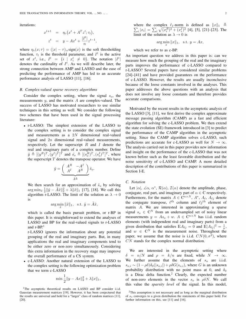
Fig. 1. Comparison of the phase transition curve of the r-BP and c-BP. Whenall the non-zero real and imaginary parts of the signal are grouped, the phasetransition of c-BP outperforms that of r-BP.

2) Noisy measurements: Consider the problem of recover-ing so distributed according to so,i

i.i.d.∼ (1 − ρδ)δ0(|so,i|) +ρδG(so,i), from a set of noisy linear observations y = Aso+w,where wi

i.i.d.∼ CN(0, σ2). In the presence of measurementnoise exact recovery is not possible. Therefore, tuning theparameter for the highest phase transition curve does notnecessarily provide the optimal performance. In this section,we explain the optimal noise sensitivity tuning introduced in[11]. Consider the `2-norm as a measure for the reconstruc-tion error and assume that ‖x

Aα−so‖22N → MSE(ρ, δ, α, σ,G)

almost surely. Define the noise sensitivity of the algorithm Aαas

NS(ρ, δ, α) , supσ>0

supG

MSE(ρ, δ, α, σ,G)

σ2, (1)

where α denotes the tuning parameter of the algorithm Aα. Ifthe noise sensitivity is large, then the measurement noise mayseverely degrade the final reconstruction. In (1) we search forthe distribution that induces the maximum reconstruction errorto the algorithm. This ensures that for other signal distributionsthe reconstruction error is smaller. By tuning α, we may obtainbetter estimate of so. Therefore, we tune the parameter α toobtain the lowest noise sensitivity, i.e.,

NS(ρ, δ) , infα

NS(ρ, δ, α).

Based on this framework, we say that algorithmA outperformsB at a given δ and ρ if and only if NSA(δ, ρ) < NSB(δ, ρ).

E. Contributions

In this paper, we first develop the complex approximatemessage passing (CAMP) algorithm that is a simple and fastconverging iterative method for solving c-LASSO. We extendthe state evolution (SE), introduced recently as a frameworkfor accurate asymptotic predictions of the AMP performance,

IEEE TRANSACTIONS ON INFORMATION THEORY, VOL. .., NO. .., .. 4

to CAMP.4 We will then use the connection between CAMPand c-LASSO to provide an accurate asymptotic analysis ofthe c-LASSO problem. We aim to characterize the phase tran-sition curve (noise-free measurements) and noise sensitivity(noisy measurements) of c-LASSO and CAMP when the realand imaginary parts are paired, i.e., they are both zero ornon-zero simultaneously. Both criteria have been extensivelystudied for the real signals (and hence for the r-LASSO)[3], [11]. The results of our predictions are summarized inFigures 1, 2, and 3. Figure 1 compares the phase transitioncurve of c-BP and CAMP with the phase transition curveof r-BP. As we expected c-BP outperforms r-BP since itexploits the connection between the real and imaginary parts.If ρSE(δ) denotes the phase transition curve, then we alsoprove that ρSE(δ) ∼ 1

log(1/2δ) as δ → 0. Comparing this withρRSE(δ) ∼ 1

2 log(1/δ) for the r-LASSO [19], we conclude that

limδ→0

ρSE(δ)

ρRSE(δ)= 2.

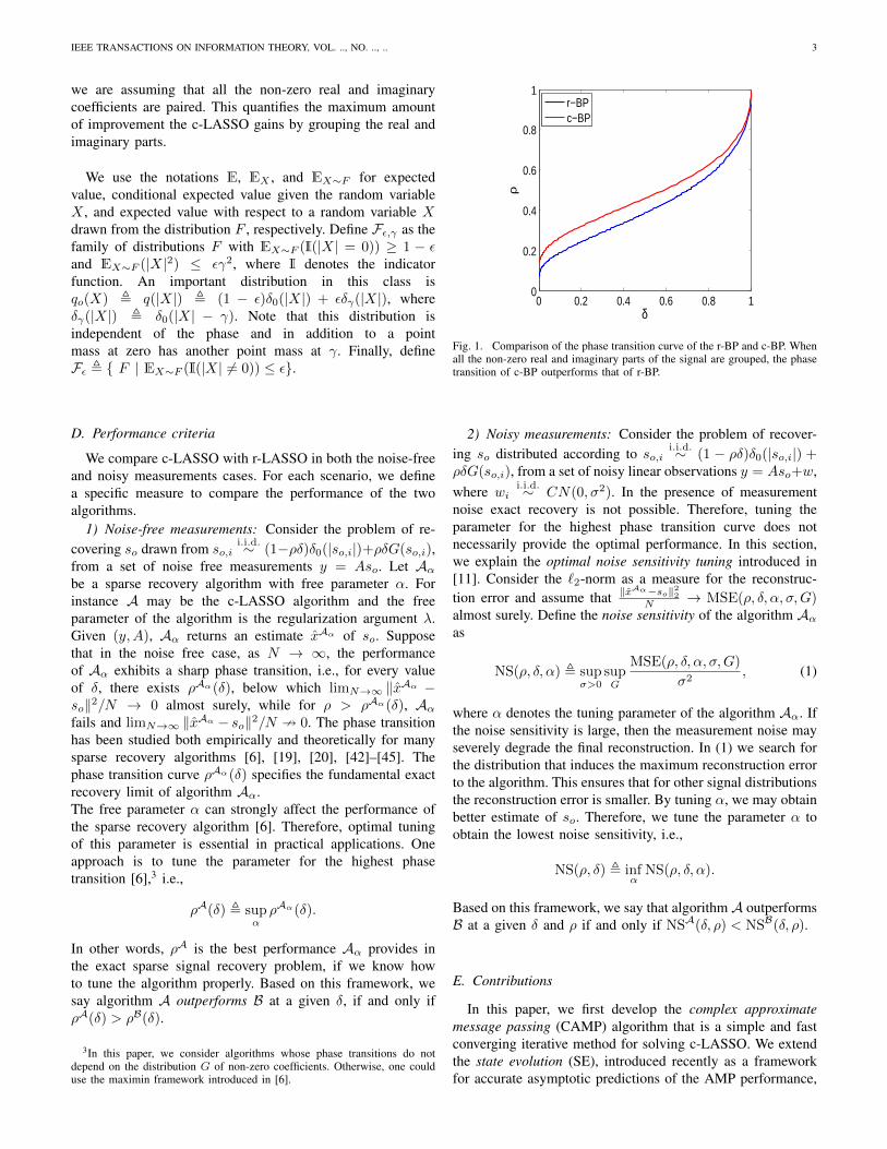
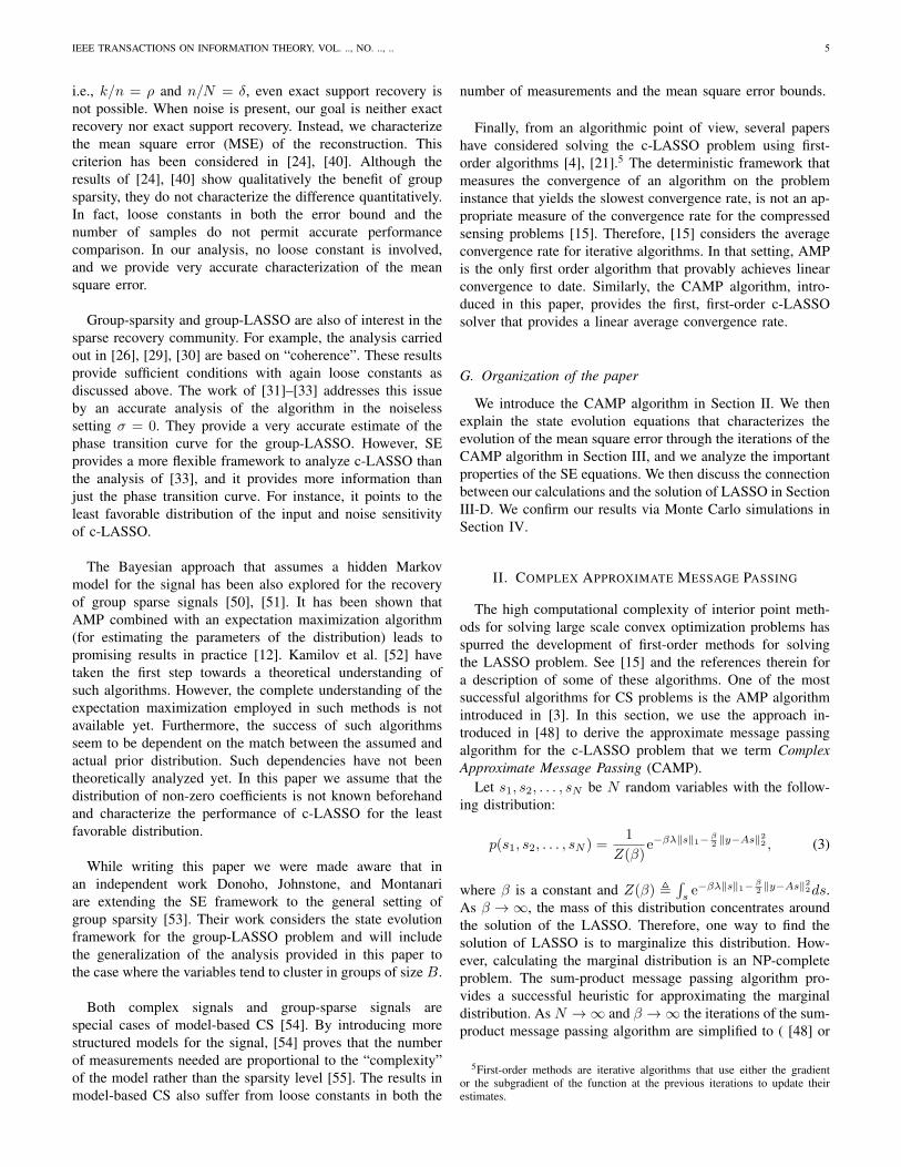
This means that, in the very high undersampling regime thec-LASSO can recover signals that are two times more densethan the signals that are recovered by r-LASSO. Figure 2exhibits the noise sensitivity of c-LASSO and CAMP. Weprove in Section III-C that, as the sparsity approaches thephase transition curve, the noise sensitivity grows up toinfinity. Finally, Figure 3 compares the contour plots of thenoise sensitivity of c-LASSO with those of the r-LASSO. Forthe fixed value noise sensitivity, the level set of the c-LASSOis higher than that of r-LASSO. It is worth noting that thesame comparisons hold between CAMP and AMP, as we willclarify in Section III-D.

F. Related work

The state evolution framework used in this paper wasfirst introduced in [3]. Deriving the phase transition andnoise sensitivity of the LASSO for real-valued signals andreal-valued measurements from SE is due to [11]; see [47]for more comprehensive discussion. Finally, the derivation ofAMP from the full sum-product message passing is due to[48]. Our main contribution in this paper is to extend theseresults to the complex setting. Not only is the analysis of thestate evolution more challenging in this setting, but it alsoprovides new insights on the performance of c-LASSO thathave not been available. For instance, the noise sensitivity ofc-LASSO has not previously been determined.

The recovery of sparse complex signals is a special caseof group-sparsity or block-sparsity, where all the groups arenon-overlapping and have size 2. According to the groupsparsity assumption, the non-zero elements of the signal tendto occur in groups or clusters. One of the algorithms used in

4Note that SE has been proved to be accurate only for the case of Gaussianmeasurement matrices [16], [46]. But, extensive simulations have confirmedits accuracy for a large class of random measurement matrices [3], [11].The results of our paper are also provably correct for complex Gaussianmeasurement matrices. But, our simulations confirm that they hold for broaderset of matrices.

δ

ρ

8

4

2

1

0.50.25

0.125

0.1 0.2 0.3 0.4 0.5 0.6 0.7 0.8 0.9

0.1

0.2

0.3

0.4

0.5

0.6

0.7

0.8

0.9

1

Fig. 2. Contour lines of noise sensitivity in the (δ, ρ) plane. The black curveis the phase transition curve at which the noise sensitivity is infinite. Thecolored lines display the level sets of NS(ρ, δ) = 0.125, 0.25, 0.5, 1, 2, 4, 8.

0.125

0.5

2

0.125

0.52

δ

ρ

0.2 0.4 0.6 0.8

0.1

0.2

0.3

0.4

0.5

0.6

0.7

0.8

0.9

Fig. 3. Comparison of the noise sensitivity of r-LASSO with the noisesensitivity of c-LASSO. The colored solid lines present the level sets of theNS(ρ, δ) = 0.125, 0.5, 2 for the c-LASSO, and the colored dotted linesdisplay the same level sets for the r-LASSO.

this context is the group-LASSO [35], [37]. Consider a signalso ∈ RN . Partition the indices of so into m groups g1, . . . , gm.The group-LASSO algorithm minimizes the following costfunction:

minx

1

2‖y −Ax‖22 +

m∑i=1

λi‖xgi‖2, (2)

where the λi’s are regularization parameters.The group-Lasso algorithm has been extensively studied in

the literature [24]–[41]. We briefly review several papers andemphasize the differences from our work. [38] analyzes theconsistency of the group LASSO estimator in the presence ofnoise. Fixing the signal so, it provides conditions under whichthe group LASSO is consistent as n→∞. [39], [49] considera weak notion of consistency, i.e., exact support recovery.However, [49] proves that in the setting we are interested in,

IEEE TRANSACTIONS ON INFORMATION THEORY, VOL. .., NO. .., .. 5

i.e., k/n = ρ and n/N = δ, even exact support recovery isnot possible. When noise is present, our goal is neither exactrecovery nor exact support recovery. Instead, we characterizethe mean square error (MSE) of the reconstruction. Thiscriterion has been considered in [24], [40]. Although theresults of [24], [40] show qualitatively the benefit of groupsparsity, they do not characterize the difference quantitatively.In fact, loose constants in both the error bound and thenumber of samples do not permit accurate performancecomparison. In our analysis, no loose constant is involved,and we provide very accurate characterization of the meansquare error.

Group-sparsity and group-LASSO are also of interest in thesparse recovery community. For example, the analysis carriedout in [26], [29], [30] are based on “coherence”. These resultsprovide sufficient conditions with again loose constants asdiscussed above. The work of [31]–[33] addresses this issueby an accurate analysis of the algorithm in the noiselesssetting σ = 0. They provide a very accurate estimate of thephase transition curve for the group-LASSO. However, SEprovides a more flexible framework to analyze c-LASSO thanthe analysis of [33], and it provides more information thanjust the phase transition curve. For instance, it points to theleast favorable distribution of the input and noise sensitivityof c-LASSO.

The Bayesian approach that assumes a hidden Markovmodel for the signal has been also explored for the recoveryof group sparse signals [50], [51]. It has been shown thatAMP combined with an expectation maximization algorithm(for estimating the parameters of the distribution) leads topromising results in practice [12]. Kamilov et al. [52] havetaken the first step towards a theoretical understanding ofsuch algorithms. However, the complete understanding of theexpectation maximization employed in such methods is notavailable yet. Furthermore, the success of such algorithmsseem to be dependent on the match between the assumed andactual prior distribution. Such dependencies have not beentheoretically analyzed yet. In this paper we assume that thedistribution of non-zero coefficients is not known beforehandand characterize the performance of c-LASSO for the leastfavorable distribution.

While writing this paper we were made aware that inan independent work Donoho, Johnstone, and Montanariare extending the SE framework to the general setting ofgroup sparsity [53]. Their work considers the state evolutionframework for the group-LASSO problem and will includethe generalization of the analysis provided in this paper tothe case where the variables tend to cluster in groups of size B.

Both complex signals and group-sparse signals arespecial cases of model-based CS [54]. By introducing morestructured models for the signal, [54] proves that the numberof measurements needed are proportional to the “complexity”of the model rather than the sparsity level [55]. The results inmodel-based CS also suffer from loose constants in both the

number of measurements and the mean square error bounds.

Finally, from an algorithmic point of view, several papershave considered solving the c-LASSO problem using first-order algorithms [4], [21].5 The deterministic framework thatmeasures the convergence of an algorithm on the probleminstance that yields the slowest convergence rate, is not an ap-propriate measure of the convergence rate for the compressedsensing problems [15]. Therefore, [15] considers the averageconvergence rate for iterative algorithms. In that setting, AMPis the only first order algorithm that provably achieves linearconvergence to date. Similarly, the CAMP algorithm, intro-duced in this paper, provides the first, first-order c-LASSOsolver that provides a linear average convergence rate.

G. Organization of the paper

We introduce the CAMP algorithm in Section II. We thenexplain the state evolution equations that characterizes theevolution of the mean square error through the iterations of theCAMP algorithm in Section III, and we analyze the importantproperties of the SE equations. We then discuss the connectionbetween our calculations and the solution of LASSO in SectionIII-D. We confirm our results via Monte Carlo simulations inSection IV.

II. COMPLEX APPROXIMATE MESSAGE PASSING

The high computational complexity of interior point meth-ods for solving large scale convex optimization problems hasspurred the development of first-order methods for solvingthe LASSO problem. See [15] and the references therein fora description of some of these algorithms. One of the mostsuccessful algorithms for CS problems is the AMP algorithmintroduced in [3]. In this section, we use the approach in-troduced in [48] to derive the approximate message passingalgorithm for the c-LASSO problem that we term ComplexApproximate Message Passing (CAMP).

Let s1, s2, . . . , sN be N random variables with the follow-ing distribution:

p(s1, s2, . . . , sN ) =1

Z(β)e−βλ‖s‖1−

β2 ‖y−As‖

22 , (3)

where β is a constant and Z(β) ,∫s

e−βλ‖s‖1−β2 ‖y−As‖

22ds.

As β →∞, the mass of this distribution concentrates aroundthe solution of the LASSO. Therefore, one way to find thesolution of LASSO is to marginalize this distribution. How-ever, calculating the marginal distribution is an NP-completeproblem. The sum-product message passing algorithm pro-vides a successful heuristic for approximating the marginaldistribution. As N →∞ and β →∞ the iterations of the sum-product message passing algorithm are simplified to ( [48] or

5First-order methods are iterative algorithms that use either the gradientor the subgradient of the function at the previous iterations to update theirestimates.

IEEE TRANSACTIONS ON INFORMATION THEORY, VOL. .., NO. .., .. 6

Chapter 5 of [47])

xt+1`→a = η

(∑b 6=a

A∗b`ztb→`; τt

),

zta→` = ya −∑j 6=`

Aajxtj→a, (4)

where η(u + iv;λ) ,(u+ iv − λ(u+iv)√

u2+v2

)+I{u2+v2>λ2} is

the proximity operator of the complex `1-norm and is calledcomplex soft thresholding. See Appendix V-A for further in-formation regarding this function. τt is the threshold parameterat time t. The choice of this parameter will be discussed inSection III-A. The per-iteration computational complexity ofthis algorithm is high, since 2nN messages xt`→a and zta→`are updated. Therefore, following [48] we assume that thereexist ∆xt`→a,∆z

t`→a = O(1/

√N) such that

xt`→a = xt` + ∆xt`→a +O(1/N),

zta→` = zta + ∆zt`→a +O(1/N). (5)

Here, the O(·) errors are uniform in the choice of the edges` → a and a → `. In other words we assume that xt`→ais independent of a and zta→` is independent of ` exceptfor an error of order 1/

√N . For further discussion of this

assumption and its validation, see [48] or Chapter 5 of [47].Let ηI and ηR be the imaginary and real parts of the complexsoft thresholding function. Furthermore, define ∂ηR

∂x and ∂ηR

∂y

as the partial derivatives of ηR with respect to the real andimaginary parts of the input respectively. ∂ηI

∂x , and ∂ηI

∂y aredefined similarly. The following theorem shows how one cansimplify the message passing as N →∞.

Proposition II.1. Suppose that (5) holds for every iteration ofthe message passing algorithm specified in (4). Then xt` andzta satisfy the following equations:

xt+1` = η

(xt` +

∑b

A∗b`ztb; τt

),

zt+1a = ya −

∑j

Aajxt+1j

−∑j

Aaj

(∂ηR

∂x

(xtj +

∑b

A∗bjztb

))R(A∗ajz

ta)

−∑j

Aaj

(∂ηR

∂y

(xtj +

∑b

A∗bjztb

))I(A∗ajz

ta)

−i∑j

Aaj

(∂ηI

∂x

(xtj +

∑b

A∗bjztb

))R(A∗ajz

ta)

−i∑j

Aaj

(∂ηI

∂y

(xtj +

∑b

A∗bjztb

))I(A∗ajz

ta).(6)

See Appendix V-B for the proof. According to PropositionII.1 and (5), for large values of N , the messages xt`→a andzta→` are close to xt` and zta in (6). Therefore, we definethe CAMP algorithm as the iterative method that starts fromx0 = 0 and z0 = y and uses the iterations specified in (6).It is important to note that Proposition II.1 does not provideany information on either the performance of the CAMP

algorithm or the connection between CAMP and c-LASSO,since message passing is a heuristic algorithm and does notnecessarily converge to the correct marginal distribution of (3).

III. FORMAL ANALYSIS OF CAMP AND C-LASSO

In this section, we explain the state evolution (SE) frame-work that predicts the performance of the CAMP and c-LASSO in the asymptotic settings. We then use this frameworkto analyze the phase transition and noise sensitivity of theCAMP and c-LASSO. The formal connection between stateevolution and CAMP/c-LASSO is discussed in Section III-D.

A. State evolution

We now conduct an asymptotic analysis of the CAMPalgorithm. As we confirm in Section III-D, the asymptoticperformance of the algorithm is tracked through a few vari-ables, called the state variables. The state of the algorithm isthe 5-tuple s = (m; δ, ρ, σ,G), where G corresponds to thedistribution of the non-zero elements of the sparse vector so,σ is the standard deviation of the measurement noise, and mis the asymptotic normalized mean square error. The thresholdparameter (threshold policy) of CAMP in its most general formcould be a function of the state of the algorithm τ(s). Definenpi(m;σ, δ) , σ2 + m

δ . The mean square error (MSE) mapis defined as

Ψ(s, τ(s)) ,

E|η(X +√

npi(m,σ, δ)Z1 + i√

npi(m,σ, δ)Z2; τ(s))−X|2,

where Z1, Z2 ∼ N(0, 1/2) and X ∼ (1−ρδ)δ0(|x|)+ρδG(x)are independent random variables. Note that G is a probabilitydistribution on C. In the rest of this paper, we consider thethresholding policy τ(s) = τ

√npi(m,σ, δ), where the con-

stant τ is yet to be tuned according to the schemes introducedin Sections I-D1 and I-D2. When we use this thresholdingpolicy we may equivalently write Ψ(s, τ(s)) as Ψ(s, τ). Thisthresholding policy is the same as the thresholding policyintroduced in [3], [11]. When the parameters δ, ρ, σ, τ andG are clear from the context, we denote the MSE map byΨ(m). SE is the evolution of m (starting from t = 0 andm0 = E(|X|2)) by the rule

mt+1 = Ψ(mt)

, E∣∣∣η(X +

√npitZ1 +i

√npitZ2; τ

√npit

)−X

∣∣∣2, (7)

where npit , npi(mt, σ, δ). As will be described in SectionIII-D, this equation tracks the normalized MSE of the CAMPalgorithm in the asymptotic setting n,N →∞ and n/N → δ.In other words, if mt is the MSE of the CAMP algorithm atiteration t, the mt+1, calculated by (7), is the MSE of CAMPat iteration t+ 1.

Definition III.1. Let Ψ be almost everywhere differentiable.m∗ is called a fixed point of Ψ if and only if Ψ(m∗) = m∗.Furthermore, a fixed point is called stable if dΨ(m)

dm

∣∣∣m=m∗

<

1, and unstable if dΨ(m)dm

∣∣∣m=m∗

> 1.

IEEE TRANSACTIONS ON INFORMATION THEORY, VOL. .., NO. .., .. 7

It is clear that if m∗ is the unique stable fixed point of the Ψfunction, then mt → m∗ as t→∞. Also, if all the fixed pointsof Ψ are unstable, then mt →∞ as t→∞. Define µ , |X|and θ , ]X . Let G(µ, θ) denote the probability densityfunction of X and define G(µ) ,

∫G(µ, θ)dθ as the marginal

distribution of µ. The next lemma shows that in order toanalyze the state evolution function we only need to considerthe amplitude distribution. This substantially simplifies ouranalysis of SE in the next sections.

Lemma III.2. The MSE map does not depend on the phasedistribution of the input signal, i.e.,

Ψ(m, δ, ρ, σ,G(µ, θ), τ) = Ψ(m, δ, ρ, σ,G(µ), τ).

See Appendix V-C for the proof.

B. Noise-free signal recovery

Consider the noise free setting with σ = 0. Suppose that SEpredicts the MSE of CAMP in the asymptotic setting (we willmake this rigorous in Section III-D). As mentioned in SectionI-D1, in order to characterize the performance of CAMP inthe noiseless setting, we first derive its phase transition curveand then optimize over τ to obtain the highest phase transitionCAMP can achieve. Fix all the state variables except for m,and ρ. The evolution of m, discriminates the following tworegions for ρ:

Region I: The values of ρ for which Ψ(m) < m for everym > 0;Region II: The complement of Region I.

Since 0 is necessarily a fixed point of the Ψ function, inRegion I mt → 0 as t→∞. The following lemma shows thatin Region II m = 0 is an unstable fixed point and thereforestarting from m0 6= 0, mt 9 0.

Lemma III.3. Let σ = 0. If ρ is in Region II, then Ψ has anunstable fixed point at zero.

Proof: We prove in Lemma V.2 that Ψ(m) is a concavefunction of m. Therefore, ρ is in Region II if and only ifdΨ(m)dm

∣∣∣m=0

> 1. This in turn indicates that 0 is an unstablefixed point.

It is also easy to confirm that Region I is of the form[0, ρSE(δ,G, τ)). As we will see in Section III-D, ρSE(δ,G, τ)determines the phase transition curve of the CAMP algorithm.According to Lemma III.2, the MSE map does not depend onthe phase distribution of the non-zero elements. The followingproposition shows that in fact ρSE is independent of G eventhough the Ψ function depends on G(µ).

Proposition III.4. ρSE(δ,G, τ) is independent of the distri-bution G.

Proof: According to Lemma V.2 in Appendix V-D, Ψis concave. Therefore, it has a stable fixed point at zero ifand only if its derivative at zero is less than 1. It is alsostraightforward (from Appendix V-D) to show that

dΨ

dm

∣∣∣∣m=0

=ρδ(1 + τ2)

δ+

1− ρδδ

E|η(Z1 + iZ2; τ)|2.

Setting this derivative to 1, it is clear that the phase transitionvalue of ρ is independent of G.

According to Proposition III.4 the only parameters thataffect ρSE are δ and the free parameter τ . Fixing δ, we tuneτ such that the algorithm achieves its highest phase transitionfor a certain number of measurements, i.e.,

ρSE(δ) , supτρSE(δ; τ).

Using SE we can calculate the optimal value of τ and ρSE(δ).

Theorem III.5. ρSE(δ) and δ satisfy the following implicitrelations:

ρSE(δ) =χ1(τ)

(1 + τ2)χ1(τ)− τχ2(τ),

δ =4(1 + τ2)χ1(τ)− 4τχ2(τ)

−2τ + 4χ2(τ),

for τ ∈ [0,∞). Here, χ1(τ) ,∫ω≥τ ω(τ − ω)e−ω

2

dω andχ2(τ) ,

∫ω>τ

ω(ω − τ)2e−ω2

.

See Appendix V-D for the proof. Figure 1 displays this phasetransition curve that is derived from the SE framework andcompares it with the phase transition of r-BP algorithm. Aswill be described later, ρSE(δ) corresponds to the phasetransition of c-LASSO. Hence the difference between ρSE(δ)and phase transition curve of r-LASSO is the benefit ofgrouping the real and imaginary parts.

It is also interesting to compare the ρSE(δ) (which as wesee later predicts the performance of c-LASSO) with the phasetransition of r-LASSO in high undersampling regime δ →0. The implicit formulation above enables us to calculate theasymptotic performance of the phase transition as δ → 0.

Theorem III.6. ρSE(δ) follows the asymptotic behavior

ρSE(δ) ∼ 1

log(

12δ

) , as δ → 0.

See Appendix V-E for the proof. As mentioned above, thistheorem shows that as δ → 0 the phase transition of c-BP andCAMP is two times that of the r-LASSO, which is given byρRSE ∼ 1/(2 log(1/δ)) [19]. This improvement is due to thegrouping of real and imaginary parts of the signal.

C. Noise sensitivity

In this section we characterize the noise sensitivity of SE.To achieve this goal, we first discuss the risk of the complexsoft thresholding function. The properties of this risk play animportant role in the discussion of the noise sensitivity of SEin Section III-C2.

1) Risk of soft thresholding: Define the risk of the softthresholding function as

r(µ, τ) , E|η(µeiθ + Z1 + iZ2; τ)−X|2,

where µ ∈ [0,∞), θ ∈ [0, 2π), and the expected valueis with respect to the two independent random variablesZ1, Z2 ∼ N(0, 1/2). It is important to note that accordingto Lemma III.2, the risk function is independent of θ. The

IEEE TRANSACTIONS ON INFORMATION THEORY, VOL. .., NO. .., .. 8

following lemma characterizes two important properties of thisrisk function:

Lemma III.7. r(µ, τ) is an increasing function of µ and aconcave function in terms of µ2.

See Appendix V-F for the proof of this lemma. We define theminimax risk of the soft thresholding function as

M [(ε) , infτ>0

supq∈Fε

E|η(X + Z1 + iZ2; τ)−X|2,

where q is the probability density function of X , and theexpected value is with respect to X , Z1 and Z2.

Note that q ∈ Fε implies that q has a point mass of 1− ε atzero; see Section I-C for more information. In the next sectionwe show a connection between this minimax risk and the noisesensitivity of the SE. Therefore, it is important to characterizeM [(ε).

Proposition III.8. The minimax risk of the soft thresholdingfunction satisfies

M [(ε) = infτ

2(1− ε)∫ ∞w=τ

w(w − τ)2e−w2

dw + ε(1 + τ2).

(8)

See Appendix V-G for the proof. It is important to notethat the quantities in (8) can be easily calculated in terms ofthe density and distribution function of a normal random vari-able. Therefore, a simple computer program may accuratelycalculate the value of M [(ε) for any ε.

The proof provided for Proposition III.8 also proves thefollowing proposition. We will discuss the importance of thisresult for compressed sensing problems in the next section.

Proposition III.9. The maximum of the risk function,maxq∈Fε,γ E|η(X + Z1 + iZ2; τ) − X|2, is achieved onq(X) = (1− ε)δ0(|X|) + εδγ(|X|).

First, note that the maximizing distribution (or least favor-able distribution) is independent of the threshold parameter.Second, note that the maximizing distribution is not uniquesince we have already proved that the phase distribution doesnot affect the risk function.

2) Noise sensitivity of state evolution: As mentioned inSection III-A, in the presence of measurement noise, SE isgiven by

mt+1 = Ψ(mt)

= E|η(X +√

npiZ1 + i√

npiZ2; τ√

npi)−X|2,

where npi = σ2 + mtδ . As mentioned above, mt characterizes

the asymptotic MSE of CAMP at iteration t. Therefore, thefinal solution of the CAMP algorithm converges to one ofthe stable fixed points of the Ψ function. The next theoremsuggests that the stable fixed point is unique, and therefore nomatter where the algorithm starts from it will always convergeto the same MSE.

Lemma III.10. Ψ(m) has a unique stable fixed point to whichthe sequence of {mt} converges.

We call the fixed point in Lemma III.10fMSE(σ2, δ, ρ,G, τ). According to Section I-D2, wedefine the minimax noise sensitivity as

NSSE(δ, ρ) , minτ

supσ>0

supq∈Fε

fMSE(σ2, δ, ρ,G, τ)/σ2.

The noise sensitivity of SE can be easily evaluated fromM [(ε). The following theorem characterizes this relation.

Theorem III.11. Let ρMSE(δ) be the value of ρ satisfyingM [(ρδ) = δ. Then, for ρ < ρMSE we have

NSSE(δ, ρ) =M [(δρ)

1−M [(δρ)/δ,

and for ρ > ρMSE(δ), NSSE(δ, ρ) =∞.

The proof of this theorem follows along the same lines as theproof of Proposition 3.1 in [11], and therefore we skip it forthe sake of brevity. The contour lines of this noise sensitivityfunction are displayed in Figure 2.

Similar arguments as those presented in Proposition 3.1 in[11] combined with Proposition III.9 prove the following.

Proposition III.12. The maximum of the formal MSE,maxq∈Fε,γ fMSE(σ2, δ, ρ,G, τ) is achieved by q = (1 −ε)δ0(|X|) + εδγ(|X|), independent of σ and τ .

Again we emphasize that the maximizing or least favorabledistribution is not unique. Note that the least favorable distri-bution provides a simple approach for designing and settingthe parameters of CS systems [8]: We design the system suchthat it performs well on the least favorable distribution, and itis then guaranteed that the system will perform as well (or inmany cases better) on all other input distributions.

As a final remark we note that ρMSE(δ) equals ρSE(δ) asproved next.

Proposition III.13. For every δ ∈ [0, 1] we have

ρMSE(δ) = ρSE(δ).

Proof: The proof is a simple comparison of the formulas.We first know that ρMSE is derived from the followingequation

minτ

2(1− ρδ)∫ω>τ

ω(ω − τ)2e−ω2

dω + ρδ(1 + τ2) = δ.

On the other hand, since Ψ(m) is a concave function of m,ρSE(δ, τ) is derived from dΨ(m)

dm

∣∣∣m=0

= 1. This derivative isequal to

dΨ(m)

dm

∣∣∣∣m=0

=2(1− ρδ)

δ

∫ω>τ

ω(ω−τ)2e−ω2

dω+ρδ

δ(1+τ2).

Also, ρSE(δ) = supτ ρSE(τ, δ). However, in order to obtainthe highest ρ we should minimize the above expression overτ . Therefore, both ρSE(δ) and ρMSE(δ) satisfy the sameequations and thus are exactly equal.

IEEE TRANSACTIONS ON INFORMATION THEORY, VOL. .., NO. .., .. 9

D. Connection between the state evolution, CAMP, and c-LASSO

There is a strong connection between the SE framework,the CAMP algorithm, and c-LASSO. Recently, [16] provedthat SE predicts the asymptotic performance of the AMPalgorithm when the measurement matrix is i.i.d. Gaussian. Theresult also holds for complex Gaussian matrices and complexinput vectors. As in [3], we conjecture that the SE predictionsare correct for a “large” class of random matrices. We showevidence of this claim in Section IV. Here, for the sake ofcompleteness, we quote the result of [16] in the complexsetting. Let γ : C2 → R be a pseudo-Lipschitz function.6 Tomake the presentation clear we consider a simplified versionof Definition 1 in [46].

Definition III.14. A sequence of instances{so(N), A(N), w(N)}, indexed by the ambient dimension N ,is called a converging sequence if the following conditionshold:

- The elements of so(N) ∈ RN are i.i.d. drawn from (1−ρδ)δ0(|so,i|) + ρδG(so,i).

- The elements of w(N) ∈ Rn (n = δN ) are i.i.d. drawnfrom N(0, σ2

w).- The elements of A(N) ∈ Rn×N are i.i.d. drawn from a

complex Gaussian distribution.

Theorem III.15. Consider a converging sequence{so(N), A(N), w(N)}. Let xt(N) be the estimate ofthe CAMP algorithm at iteration t. For any pseudo Lipschitzfunction γ : C2 → R we have

limN→∞

1

N

N∑i=1

γ(xti, so,i)

= Eγ

(η

(X +

√npitZ1 + i

√npitZ2; τ

√npit

), X

)almost surely, where Z1 + iZ2 ∼ CN(0, 1) and X ∼(1−ρδ)δ0(|so,i|)+ρδG(so,i) are independent complex randomvariables. Also, npit , σ2 +mt/δ, where mt satisfies (7).

The proof of this theorem is similar to the proof ofTheorem 1 in [16] and hence is skipped here.

It is also straightforward to extend the result of [11] and [46]on the connection of message passing algorithms and LASSOto the complex setting. For a given value of τ suppose thatthe fixed point of the state evolution is denoted by m∗. Defineλ(τ) as

λ(τ),τ√m∗(

1− 1

2δE

(∂ηR

∂x+∂ηI

∂y

)), (9)

where

∂ηR

∂x,

∂ηR

∂x

(X +

√m∗Z1+i

√m∗Z2; τ

√m∗),

∂ηI

∂y,

∂ηI

∂y

(X +

√m∗Z1 + i

√m∗Z2; τ

√m∗),

6γ : C2 → R is pseudo-Lipschitz if and only if |ψ(x)− ψ(y)| ≤ L(1 +‖x‖2 + ‖y‖2)‖x− y‖2.

and E is with respect to independent random variables Z1 +iZ2 ∼ CN(0, 1) and X ∼ (1 − ρδ)δ0(|so,i|) + ρδG(so,i).The following theorem establishes the connection between thesolution of LASSO and the state evolution equation.

Theorem III.16. Consider a converging sequence{so(N), A(N), w(N)}. Let xλ(τ)(N) be the solution ofLASSO. Then, for any pseudo Lipschitz function γ : C2 → R

we have

limN→∞

1

N

N∑i=1

γ(xλ(τ)i (N), so,i)

= Eγ(η(X +

√npi∗Z1 + i

√npi∗Z2; τ

√npi∗

), X)

almost surely, where Z1 + iZ2 ∼ CN(0, 1) and X ∼(1−ρδ)δ0(|so,i|)+ρδG(so,i) are independent complex randomvariables. npi∗ , σ2 +m∗/δ, where m∗ is the fixed point of(7).

The proof of the theorem is similar to the proof of Theorem1.4 in [46] and hence is skipped here.

Note that according to Theorems III.15 and III.16, SEpredicts the dynamic of the AMP algorithm and the solutionof LASSO accurately in the asymptotic settings.

E. Discussion

1) Convergence rate of CAMP: In this section we brieflydiscuss the convergence rate of the CAMP algorithm. In thisrespect our results are straightforward extension of the analysisin [15]. But, for the sake of completeness, we mention a fewhighlights. Let {mt}∞t=1 be a sequence of MSE generated ac-cording to state evolution (7) for X ∼ (1−ε)δ0(|X|)+εG(X),τ , and σ2 = 0. The following proposition provides an upperbound on mt as a function of iteration t.

Theorem III.17. Let {mt}∞t=1 be a sequence of MSEs gener-ated according to SE. Then

mt ≤(dΨ(m)

dm

∣∣∣∣m=0

)tm0.

Proof: Since according to Lemma V.2 Ψ(m) is concave,we have Ψ(m) ≤ dΨ(m)

dm

∣∣∣m=0

m. Hence at every iteration,

m is attenuated by dΨ(m)dm

∣∣∣m=0

. After t iterations we have

mt ≤(dΨ(m)dm

∣∣∣m=0

)tm0.

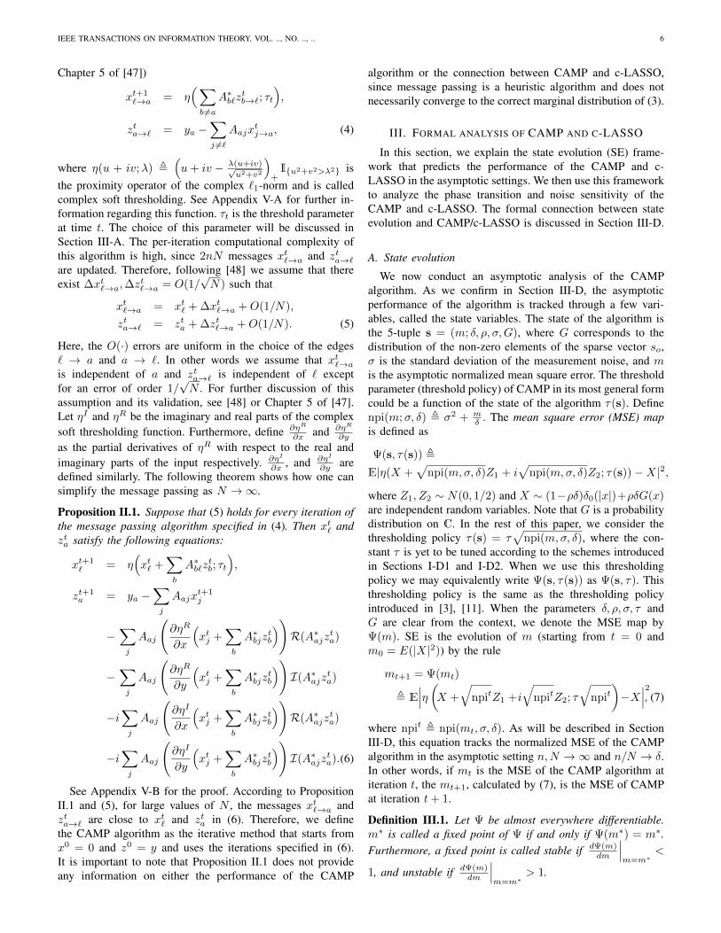
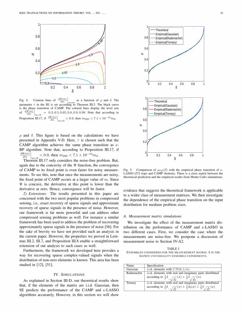
According to Theorem III.17 the convergence rate of CAMPis linear (in the asymptotic setting).7 In fact, due to theconcavity of the Ψ function, CAMP converges faster forlarge values of MSE m. As m reaches zero the convergencerate decreases towards the rate predicted by this theorem.Theorem III.17 provides an upper bound on the number ofiterations the algorithm requires to reach to a certain accuracy.Figure 4 exhibits the value of dΨ(m)

dm

∣∣∣m=0

as a function of

7If the measurement matrix is not i.i.d. random CAMP does not necessarilyconverge at this rate. This is due to the fact that state evolution does notnecessarily hold for arbitrary matrices.

IEEE TRANSACTIONS ON INFORMATION THEORY, VOL. .., NO. .., .. 10

δ

ρ

0.3

0.5

0.65

0.8

0.9

0.98

0.2 0.4 0.6 0.8 1

0.2

0.4

0.6

0.8

1

Fig. 4. Contour lines of dΨ(m)dm

∣∣∣m=0

as a function of ρ and δ. Theparameter τ in the SE is set according to Theorem III.5. The black curveis the phase transition of CAMP. The colored lines display the level setsof dΨ(m)

dm

∣∣∣m=0

= 0.3, 0.5, 0.65, 0.8, 0.9, 0.98. Note that according to

Proposition III.17, if dΨ(m)dm

∣∣∣m=0

< 0.9, then m200 < 7.1× 10−10m0.

ρ and δ. This figure is based on the calculations we havepresented in Appendix V-D. Here, τ is chosen such that theCAMP algorithm achieves the same phase transition as c-BP algorithm. Note that, according to Proposition III.17, ifdΨ(m)dm

∣∣∣m=0

< 0.9, then m200 < 7.1× 10−10m0.Theorem III.17 only considers the noise-free problem. But,

again due to the concavity of the Ψ function, the convergenceof CAMP to its fixed point is even faster for noisy measure-ments. To see this, note that once the measurements are noisy,the fixed point of CAMP occurs at a larger value of m. SinceΨ is concave, the derivative at this point is lower than thederivative at zero. Hence, convergence will be faster.

2) Extensions: The results presented in this paper areconcerned with the two most popular problems in compressedsensing, i.e., exact recovery of sparse signals and approximaterecovery of sparse signals in the presence of noise. However,our framework is far more powerful and can address othercompressed sensing problems as well. For instance a similarframework has been used to address the problem of recoveringapproximately sparse signals in the presence of noise [56]. Forthe sake of brevity we have not provided such an analysis inthe current paper. However, the properties we proved in Lem-mas III.2, III.7, and Proposition III.8 enable a straightforwardextension of our analysis to such cases as well.

Furthermore, the framework we developed here provides away for recovering sparse complex-valued signals when thedistribution of non-zero elements is known. This area has beenstudied in [12], [51].

IV. SIMULATIONS

As explained in Section III-D, our theoretical results showthat, if the elements of the matrix are i.i.d. Gaussian, thenSE predicts the performance of the CAMP and c-LASSOalgorithms accurately. However, in this section we will show

0 0.2 0.4 0.6 0.8 10

0.2

0.4

0.6

0.8

1

δ

ρ

TheoreticalEmpirical(Gaussian)Empirical(Rademacher)Empirical(Ternary)

0 0.2 0.4 0.6 0.8 10

0.2

0.4

0.6

0.8

1

δ

ρ

TheoreticalEmpirical(Gaussian)Empirical(Rademacher)Empirical(Ternary)

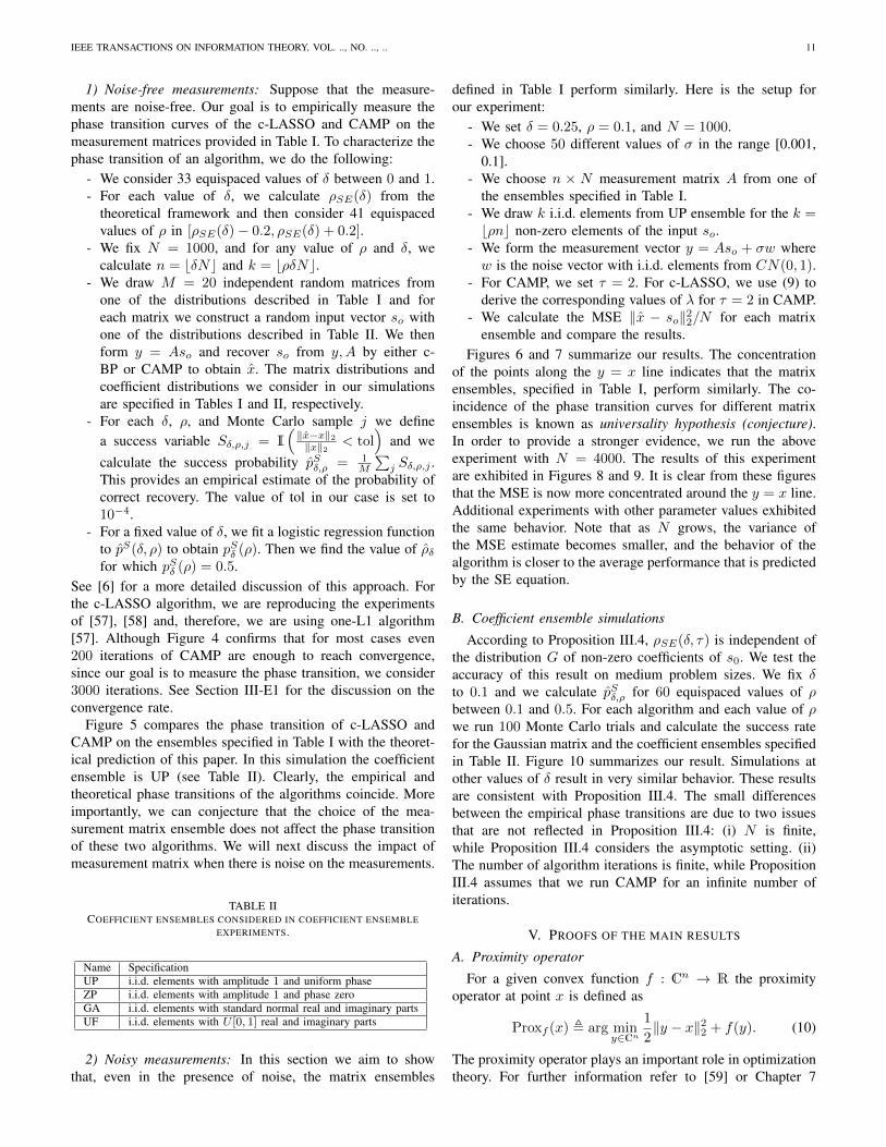
Fig. 5. Comparison of ρSE(δ) with the empirical phase transition of c-LASSO [57] (top) and CAMP (bottom). There is a close match between thetheoretical prediction and the empirical results from Monte Carlo simulations.

evidence that suggests the theoretical framework is applicableto a wider class of measurement matrices. We then investigatethe dependence of the empirical phase transition on the inputdistribution for medium problem sizes.

A. Measurement matrix simulations

We investigate the effect of the measurement matrix dis-tribution on the performance of CAMP and c-LASSO intwo different cases. First, we consider the case where themeasurements are noise-free. We postpone a discussion ofmeasurement noise to Section IV-A2.

TABLE IENSEMBLES CONSIDERED FOR THE MEASUREMENT MATRIX A IN THE

MATRIX UNIVERSALITY ENSEMBLE EXPERIMENTS.

Name SpecificationGaussian i.i.d. elements with CN(0, 1/n)Rademacher i.i.d. elements with real and imaginary parts distributed

according to 12δ−√

12n

(x) + 12δ√ 1

2n

(x)

Ternary i.i.d. elements with real and imaginary parts distributedaccording to 1

3δ−√

32n

(x) + 13δ0(x) +

13δ√ 3

2n

(x)

IEEE TRANSACTIONS ON INFORMATION THEORY, VOL. .., NO. .., .. 11

1) Noise-free measurements: Suppose that the measure-ments are noise-free. Our goal is to empirically measure thephase transition curves of the c-LASSO and CAMP on themeasurement matrices provided in Table I. To characterize thephase transition of an algorithm, we do the following:

- We consider 33 equispaced values of δ between 0 and 1.- For each value of δ, we calculate ρSE(δ) from the

theoretical framework and then consider 41 equispacedvalues of ρ in [ρSE(δ)− 0.2, ρSE(δ) + 0.2].

- We fix N = 1000, and for any value of ρ and δ, wecalculate n = bδNc and k = bρδNc.

- We draw M = 20 independent random matrices fromone of the distributions described in Table I and foreach matrix we construct a random input vector so withone of the distributions described in Table II. We thenform y = Aso and recover so from y,A by either c-BP or CAMP to obtain x. The matrix distributions andcoefficient distributions we consider in our simulationsare specified in Tables I and II, respectively.

- For each δ, ρ, and Monte Carlo sample j we definea success variable Sδ,ρ,j = I

(‖x−x‖2‖x‖2 < tol

)and we

calculate the success probability pSδ,ρ = 1M

∑j Sδ,ρ,j .

This provides an empirical estimate of the probability ofcorrect recovery. The value of tol in our case is set to10−4.

- For a fixed value of δ, we fit a logistic regression functionto pS(δ, ρ) to obtain pSδ (ρ). Then we find the value of ρδfor which pSδ (ρ) = 0.5.

See [6] for a more detailed discussion of this approach. Forthe c-LASSO algorithm, we are reproducing the experimentsof [57], [58] and, therefore, we are using one-L1 algorithm[57]. Although Figure 4 confirms that for most cases even200 iterations of CAMP are enough to reach convergence,since our goal is to measure the phase transition, we consider3000 iterations. See Section III-E1 for the discussion on theconvergence rate.

Figure 5 compares the phase transition of c-LASSO andCAMP on the ensembles specified in Table I with the theoret-ical prediction of this paper. In this simulation the coefficientensemble is UP (see Table II). Clearly, the empirical andtheoretical phase transitions of the algorithms coincide. Moreimportantly, we can conjecture that the choice of the mea-surement matrix ensemble does not affect the phase transitionof these two algorithms. We will next discuss the impact ofmeasurement matrix when there is noise on the measurements.

TABLE IICOEFFICIENT ENSEMBLES CONSIDERED IN COEFFICIENT ENSEMBLE

EXPERIMENTS.

Name SpecificationUP i.i.d. elements with amplitude 1 and uniform phaseZP i.i.d. elements with amplitude 1 and phase zeroGA i.i.d. elements with standard normal real and imaginary partsUF i.i.d. elements with U [0, 1] real and imaginary parts

2) Noisy measurements: In this section we aim to showthat, even in the presence of noise, the matrix ensembles

defined in Table I perform similarly. Here is the setup forour experiment:

- We set δ = 0.25, ρ = 0.1, and N = 1000.- We choose 50 different values of σ in the range [0.001,

0.1].- We choose n × N measurement matrix A from one of

the ensembles specified in Table I.- We draw k i.i.d. elements from UP ensemble for the k =bρnc non-zero elements of the input so.

- We form the measurement vector y = Aso + σw wherew is the noise vector with i.i.d. elements from CN(0, 1).

- For CAMP, we set τ = 2. For c-LASSO, we use (9) toderive the corresponding values of λ for τ = 2 in CAMP.

- We calculate the MSE ‖x − so‖22/N for each matrixensemble and compare the results.

Figures 6 and 7 summarize our results. The concentrationof the points along the y = x line indicates that the matrixensembles, specified in Table I, perform similarly. The co-incidence of the phase transition curves for different matrixensembles is known as universality hypothesis (conjecture).In order to provide a stronger evidence, we run the aboveexperiment with N = 4000. The results of this experimentare exhibited in Figures 8 and 9. It is clear from these figuresthat the MSE is now more concentrated around the y = x line.Additional experiments with other parameter values exhibitedthe same behavior. Note that as N grows, the variance ofthe MSE estimate becomes smaller, and the behavior of thealgorithm is closer to the average performance that is predictedby the SE equation.

B. Coefficient ensemble simulations

According to Proposition III.4, ρSE(δ, τ) is independent ofthe distribution G of non-zero coefficients of s0. We test theaccuracy of this result on medium problem sizes. We fix δto 0.1 and we calculate pSδ,ρ for 60 equispaced values of ρbetween 0.1 and 0.5. For each algorithm and each value of ρwe run 100 Monte Carlo trials and calculate the success ratefor the Gaussian matrix and the coefficient ensembles specifiedin Table II. Figure 10 summarizes our result. Simulations atother values of δ result in very similar behavior. These resultsare consistent with Proposition III.4. The small differencesbetween the empirical phase transitions are due to two issuesthat are not reflected in Proposition III.4: (i) N is finite,while Proposition III.4 considers the asymptotic setting. (ii)The number of algorithm iterations is finite, while PropositionIII.4 assumes that we run CAMP for an infinite number ofiterations.

V. PROOFS OF THE MAIN RESULTS

A. Proximity operator

For a given convex function f : Cn → R the proximityoperator at point x is defined as

Proxf (x) , arg miny∈Cn

1

2‖y − x‖22 + f(y). (10)

The proximity operator plays an important role in optimizationtheory. For further information refer to [59] or Chapter 7

IEEE TRANSACTIONS ON INFORMATION THEORY, VOL. .., NO. .., .. 12

0 0.5 1 1.5

x 10−3

0

0.5

1

1.5x 10

−3

Mean Square Error (Rademacher)

Me

an

Sq

ua

re E

rro

r (G

au

ssia

n)

0 0.5 1 1.5

x 10−3

0

0.5

1

1.5x 10

−3

Mean Square Error (Ternary)

Me

an

Sq

ua

re E

rro

r (G

au

ssia

n)

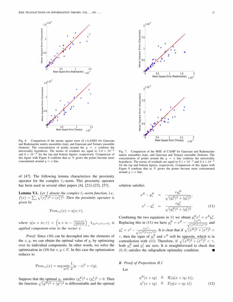
Fig. 6. Comparison of the means square error of c-LASSO for Gaussianand Rademacher matrix ensembles (top), and Gaussian and Ternary ensemble(bottom). The concentration of points around the y = x confirms theuniversality hypothesis. The norms of residuals are equal to 5.9 × 10−4

and 6 × 10−4 for the top and bottom figures, respectively. Comparison ofthis figure with Figure 8 confirms that as N grows the points become moreconcentrated around y = x line.

of [47]. The following lemma characterizes the proximityoperator for the complex `1-norm. This proximity operatorhas been used in several other papers [4], [21]–[23], [57].

Lemma V.1. Let f denote the complex `1-norm function, i.e.,f(x) =

∑i

√(xRi )2 + (xIi )

2. Then the proximity operator isgiven by

Proxτf (x) = η(x; τ),

where η(u + iv; τ) =(u+ iv − τ(u+iv)√

u2+v2

)+

1{u2+v2>τ2} isapplied component-wise to the vector x.

Proof: Since (10) can be decoupled into the elements ofthe x, y, we can obtain the optimal value of y, by optimizingover its individual components. In other words, we solve theoptimization in (10) for x, y ∈ C. In this case the optimizationreduces to

Proxτf (x) = arg miny∈C

1

2|y − x|2 + τ |y|.

Suppose that the optimal y∗ satisfies (yR∗ )2 +(yI∗)2 > 0. Then

the function√

(yR)2 + (yI)2 is differentiable and the optimal

0 0.5 1 1.5 2

x 10−3

0

0.5

1

1.5

2x 10

−3

Mean Square Error (Rademacher)

Me

an

Sq

ua

re E

rro

r (G

au

ssia

n)

0 0.5 1 1.5 2

x 10−3

0

0.5

1

1.5

2x 10

−3

Mean Square Error (Ternary)M

ea

n S

qu

are

Err

or

(Ga

ussia

n)

Fig. 7. Comparison of the MSE of CAMP for Gaussian and Rademachermatrix ensembles (top), and Gaussian and Ternary ensemble (bottom). Theconcentration of points around the y = x line confirms the universalityhypothesis. The norms of residuals are equal to 9.1× 10−4 and 9.4× 10−4

for the top and bottom figures, respectively. Comparison of this figure withFigure 9 confirms that as N grows the points become more concentratedaround y = x line.

solution satisfies

xR − yR∗ =τyR∗√

(yR∗ )2 + (yI∗)2,

xI − yI∗ =τyI∗√

(yR∗ )2 + (yI∗)2. (11)

Combining the two equations in 11 we obtain yR∗ xI = xRyI∗ .

Replacing this in (11) we have yR∗ = xR − τ |xR|√(xR)2+(xI)2

and

yI∗ = xI− τ |xI |√(xR)2+(xI)2

. It is clear that if√

(xR)2 + (xI)2 <

τ , then the signs of yR∗ and xR will be opposite, which is incontradiction with (11). Therefore, if

√(xR)2 + (xI)2 < τ ,

both yR∗ and yI∗ are zero. It is straightforward to check that(0, 0) satisfies the subgradient optimality condition.

B. Proof of Proposition II.1

Let

ηR(x+ iy) , R(η(x+ iy;λ)),

ηI(x+ iy) , I(η(x+ iy;λ)) (12)

IEEE TRANSACTIONS ON INFORMATION THEORY, VOL. .., NO. .., .. 13

0 0.2 0.4 0.6 0.8 1 1.2

x 10−3

0

0.2

0.4

0.6

0.8

1

1.2x 10

−3

Mean Square Error (Rademacher)

Me

an

Sq

ua

re E

rro

r (G

au

ssia

n)

0 0.2 0.4 0.6 0.8 1 1.2

x 10−3

0

0.2

0.4

0.6

0.8

1

1.2x 10

−3

Mean Square Error (Ternary)

Me

an

Sq

ua

re E

rro

r (G

au

ssia

n)

Fig. 8. Comparison of the MSE of c-LASSO for Gaussian and Rademachermatrix ensembles (top), and Gaussian and Ternary ensemble (bottom). Theconcentration of the points around the y = x line confirms the universalityhypothesis. The norms of residuals are 2.8× 10−4 and 2.3× 10−4 for thetop and bottom figures respectively. Comparison of this figure with Figure 6confirms that as N grows the data points concentrate more around y = xline.

denote the real and imaginary parts of the complex softthresholding function. Define

∂1ηR ,

∂ηR(x+ iy)

∂x,

∂2ηR ,

∂ηR(x+ iy)

∂y,

∂1ηI ,

∂ηI(x+ iy)

∂x,

∂2ηI ,

∂ηI(x+ iy)

∂y. (13)

We first simplify the expression for zta→`:

zta→` = ya −∑j∈[N ]

Aajxtj −

∑j∈[N ]

Aaj∆xtj→a︸ ︷︷ ︸

zta,

+ Aa`xt`︸ ︷︷ ︸

∆zta→`,

+O(1/N). (14)

0 0.2 0.4 0.6 0.8 1 1.2

x 10−3

0

0.2

0.4

0.6

0.8

1

1.2x 10

−3

Mean Square Error (Rademacher)

Me

an

Sq

ua

re E

rro

r (G

au

ssia

n)

0 0.2 0.4 0.6 0.8 1 1.2

x 10−3

0

0.2

0.4

0.6

0.8

1

1.2x 10

−3

Mean Square Error (Ternary)

Me

an

Sq

ua

re E

rro

r (G

au

ssia

n)

Fig. 9. Comparison of the MSE of CAMP for Gaussian and Rademachermatrix ensembles (top), and Gaussian and Ternary ensemble (bottom). Thenorms of residuals are 2× 10−4 and 1.8× 10−4, respectively. Comparisonwith Figure 7 confirms that as N grows the data points concentrate morearound y = x line.

We also use the first-order expansion of the soft thresholdingfunction to obtain

xt+1`→a

= η( ∑b∈[n]

A∗b`ztb +

∑b∈[n]

A∗b`∆ztb→` −A∗a`zta; τt

)+O

(1

N

)= η

( ∑b∈[n]

A∗b`ztb +

∑b∈[n]

A∗b`∆ztb→`; τt

)︸ ︷︷ ︸

xt`,

−R(A∗a`zta)∂1η

R( ∑b∈[n]

A∗b`ztb +

∑b∈[n]

A∗b`∆ztb→`

)−I(A∗a`z

ta)∂2η

R( ∑b∈[n]

A∗b`ztb +

∑b∈[n]

A∗b`∆ztb→`

)−R(A∗a`z

ta)∂1η

I( ∑b∈[n]

A∗b`ztb +

∑b∈[n]

A∗b`∆ztb→`

)−I(A∗a`z

ta)∂2η

I( ∑b∈[n]

A∗b`ztb +

∑b∈[n]

A∗b`∆ztb→`

)+O

(1

N

). (15)

IEEE TRANSACTIONS ON INFORMATION THEORY, VOL. .., NO. .., .. 14

0.1 0.2 0.3 0.4 0.50

0.2

0.4

0.6

0.8

1

ρ

Succ

ess

Rate

UF EmpiricalUF LOGIT FitUP EmpiricalUP LOGIT FitZP EmpiricalZP LOGIT FitGA EmpiricalGA LOGIT Fit

0.1 0.2 0.3 0.4 0.50

0.2

0.4

0.6

0.8

1

ρ

Succ

ess

Rate

UF EmpiricalUF LOGIT FitUP EmpiricalUP LOGIT FitZP EmpiricalZP LOGIT FitGA EmpiricalGA LOGIT Fit

Fig. 10. Comparison of the phase transition of c-LASSO (top) and CAMP(bottom) for different coefficient ensembles specified in Table II. δ = 0.1in this figure. These figures are in agreement with Proposition III.4 thatclaims the phase transition of CAMP and c-LASSO are independent of thedistribution of the non-zero coefficients. Simulations at other values of δ resultin similar behavior.

According to (14) ∆ztb→` = Ab`xt`. Furthermore, we assume

that the columns of the matrix are normalized. Therefore,∑bA∗b`δz

tb→` = xt`. It is also clear that

∆xt`→a

, −R(A∗a`zta)∂1η

R( ∑b∈[n]

A∗b`ztb +

∑b∈[n]

A∗b`∆ztb→`

)−I(A∗a`z

ta)∂2η

R( ∑b∈[n]

A∗biztb +

∑b∈[n]

A∗b`∆ztb→`

)−R(A∗a`z

ta)∂1η

I( ∑b∈[n]

A∗b`ztb +

∑b∈[n]

A∗b`∆ztb→`

)−I(A∗a`z

ta)∂2η

I( ∑b∈[n]

A∗b`ztb +

∑b∈[n]

A∗b`∆ztb→`

).

(16)

Also, according to (14)

zta = ya −∑j

Aajxtj −

∑j

Aaj∆xtj→a. (17)

By plugging (16) into (17), we obtain

−∑j

Aaj∆xtj→a

=∑j

AajR(A∗ajzta)∂1η

R(∑

b

A∗bjztb + xtj

)+

∑j

AajI(A∗ajzta)∂2η

R(∑

b

A∗bjztb + xtj

)+ i

∑j

AajR(A∗ajzta)∂1η

I(∑

b

A∗bjztb + xtj

)+ i

∑j

AajI(A∗ajzta)∂2η

I(∑

b

A∗bjztb + xtj

),

which completes the proof. �

C. Proof of Lemma III.2

Let µ and θ denote the amplitude and phase of the randomvariable X . Define ν ,

√npi =

√σ2 + m

δ and ζ , µν . Then

Ψ(m) = E|η(X +√

npiZ1 + i√

npiZ2; τ√

npi)−X|2

= ν2E

∣∣∣∣η(Xν + Z1 + iZ2; τ

)− X

ν

∣∣∣∣2= (1− ε)ν2E|η(Z1 + iZ2; τ)|2

+ εν2E(Eζ,θ|η(ζeiθ + Z1 + iZ2; τ)− ζeiθ|2

), (18)

where Eζ,θ denotes the conditional expectation given thevariables ζ, θ. Note that the marginal distribution of ζ dependsonly on the marginal distribution of µ. The first term in (18)is independent of the phase θ, and therefore we should provethat the second term is also independent of θ. Define

Φ(ζ, θ) , Eζ,θ(|η(ζeiθ + Z1 + iZ2; τ)− ζeiθ|2). (19)

We prove that Φ is independent of θ. For two real-valuedvariables zr and zc, define z , (zr, zc), dz , dzrdzc, and

αz ,√

(ζ cos θ + zr)2 + (ζ sin θ + zc)2,

χz , arctan

(ζ sin θ + zcζ cos θ + zr

),

cr ,ζ cos θ + zr

αz,

ci ,ζ sin θ + zc

αz.

Define the two sets Sτ , {(zr, zc) | αz < τ} and Scτ ,R2\Sτ , where “\” is the set subtraction operator. We have

Φ(ζ, θ)

=

∫z∈Sτ

ζ2 1

πe−(z2r+z2c )dz

+

∫z∈Scτ

∣∣(αz − τ)eiχz − ζ cos θ − iζ sin θ∣∣2 1

πe−(z2r+z2c )dz

=

∫z∈Sτ

ζ2 1

πe−(z2r+z2c )dz

+

∫z∈Scτ

|zr + izc − τcr − iτci|21

πe−(z2r+z2c )dz. (20)

IEEE TRANSACTIONS ON INFORMATION THEORY, VOL. .., NO. .., .. 15

The first integral in (20) corresponds to the case |ζeiθ + zr +izc| < τ . The second integral is over the values of zr and zcfor which |ζeiθ + zr + izc| ≥ τ . Define β , ζ cos θ + zr andγ , ζ sin θ + zc. We then obtain∫z∈Scτ

|zr + izc − τcr − iτci|21

πe−(z2r+z2c )dzrdzc

=

∫√β2+γ2>τ

∣∣∣β − ζ cos θ + i(γ − ζ sin θ)

− τβ√β2 + γ2

− i τγ√β2 + γ2

∣∣∣21

πe−(β−ζ cos θ)2−(γ−ζ sin θ)2dβdγ

(a)=

2π∫φ=0

∫r>τ

|(r − τ) cosφ− ζ cos θ

+i((r − τ) sinφ− ζ sin θ)|21

πe−(r cosφ−ζ cos θ)2−(r sinφ−ζ sin θ)2rdrdφ

=

2π∫φ=0

∫r>τ

[(r − τ)2 + ζ2 − 2ζ(r − τ) cos(θ − φ)]

e−r2−ζ2+2rζ cos(θ−φ)rdrdφ.

Equality (a) is the result of the change of integration variablesfrom γ and β to r ,

√β2 + γ2 and φ , arctan

(γβ

).

The periodicity of the cosine function proves that the lastintegration is independent of the phase θ. We can similarlyprove that

∫z∈Sτ ζ

2 1π e−z

2r+z2cdz is independent of θ. This

completes the proof. �

D. Proof of Theorem III.5We first prove the following lemma that simplifies the proof

of Theorem III.5.

Lemma V.2. The function Ψ(m) is concave with respect tom.

Proof: For the notational simplicity define ν ,√σ2 + m

δ , Xν , Xν , and Aν , |Xν − Z1 + iZ2|. We note

thatd2Ψ

dm2=

d

dm

(dΨ

dm

)=

d

dm

(dΨ

d(ν2)

dν2

dm

)=

1

δ

d

dm

(dΨ

dν2

)=

1

δ2

d2Ψ

d(ν2)2.

Therefore, Ψ is concave with respect to m if and only ifit is concave with respect to ν2. According to Lemma III.2the phase distribution of X does not affect the Ψ function.Therefore, we set the phase of X to zero and assume that it is apositive-valued random variable (representing the amplitude).This assumption substantially simplifies the calculations. Wehave

Ψ(ν2) = ν2E(|η(Xν + Z1 + iZ2; τ)−Xν |2

)= ν2E

(EX

(|η(Xν + Z1 + iZ2; τ)−Xν |2

)),

where EX denotes the expected value conditioned onthe random variable X . We first prove that ΨX(ν2) ,

ν2EX

(|η(Xν + Z1 + iZ2; τ)−Xν |2

)is concave with re-

spect to ν2 by proving dΨXd(ν2)2 ≤ 0. Then, since Ψ(ν2) is a

convex combination of ΨX(ν2), we conclude that Ψ(ν2) is aconcave function of ν2 as well. The rest of the proof detailsthe algebra required for calculating and simplifying d2ΨX(ν2)

d2ν2 .

Using the real and imaginary parts of the soft thresholdingfunction and its partial derivatives introduced in (12) and (13)we have

dΨX(ν2)

dν2

= EX |η (Xν + Z1 + iZ2; τ)−Xν |2

+ ν2 d

dνEX |η (Xν + Z1 + iZ2; τ)−Xν |2

dν

d(ν2)

= EX |η (Xν + Z1 + iZ2; τ)−Xν |2

+ν

2

d

dνEX |η (Xν + Z1 + iZ2; τ)−Xν |2

= EX |η (Xν + Z1 + iZ2; τ)−Xν |2

−XνEX

[ (∂1η

R(Xν + Z1 + iZ2; τ)− 1)

(ηR(Xν + Z1 + iZ2; τ)−Xν

) ]−XνEX

[ (∂1η

I(Xν + Z1 + iZ2; τ))

(ηI(Xν + Z1 + iZ2; τ)

) ],

where ∂R1 , ∂R2 , ∂I1 , and ∂I2 are defined in (13). Note that inthe above calculations, ∂2η

R and ∂2ηI did not appear, since

we assumed that X is a real-valued random variable. DefineAν ,

√(Xν + Z1)2 + Z2

2 . It is straightforward to show that

∂1ηR(Xν + Z1 + iZ2; τ) =

(1− τZ2

2

A3ν

)I(Aν > τ),

ηR(Xν + Z1 + iZ2; τ) = (Xν + Z1)

(1− τ

Aν

)I(Aν ≥ τ),

∂1ηI(Xν + Z1 + iZ2; τ) =

τ(Xν + Z1)Z2

A3ν

I(Aν ≥ τ),

ηI(Xν + Z1 + iZ2; τ) =

(Z2 −

τZ2

Aν

)I(Aν ≥ τ). (21)

For f : C → R we define ∂21f(x + iy) , ∂2f(x+iy)

∂x2 . It isstraightforward to show that

d2ΨX(ν2)

d2ν2

= −Xν3EX

[ (∂1η

R(Xν + Z1 + iZ2; τ)− 1)

(ηR(Xν + Z1 + iZ2; τ)−Xν

) ]− X

ν3EX

[ (∂1η

I(Xν + Z1 + iZ2; τ))

(ηI(Xν + Z1 + iZ2; τ)

) ]+

X

2ν3EX

[ (∂1η

R(Xν + Z1 + iZ2; τ)− 1)

(ηR(Xν + Z1 + iZ2; τ)−Xν

) ]

IEEE TRANSACTIONS ON INFORMATION THEORY, VOL. .., NO. .., .. 16

+X

2ν3EX

[ (∂1η

I(Xν + Z1 + iZ2; τ))

(ηI(Xν + Z1 + iZ2; τ)

) ]+

X2

2ν4EX

(∂1η

R(Xν + Z1 + iZ2; τ)− 1)2

+X2

2ν4EX

(∂1η

I(Xν + Z1 + iZ2; τ))2

+X2

2ν4EX

[ (∂2

1ηR(Xν + Z1 + iZ2; τ)

)(ηR(Xν + Z1 + iZ2; τ)−Xν

) ]+

X2

2ν4EX

[ (∂2

1ηI(Xν + Z1 + iZ2; τ)

)(ηI(Xν + Z1 + iZ2; τ)

) ]. (22)

Our next objective is to simplify the terms in (22). We startwith

EX

[ (∂1η

R(Xν + Z1 + iZ2; τ)− 1)

(ηR(Xν + Z1 + iZ2; τ)−Xν

) ]+EX

[ (∂1η

I(Xν + Z1 + iZ2; τ))

(ηI(Xν + Z1 + iZ2; τ)

) ]=X

νEX

(I(Aν ≤ τ) +

τZ22

A3ν

I(Aν ≥ τ)

). (23)

Similarly,

EX(∂1η

R(Xν + Z1 + iZ2; τ)− 1)2

+ EX(∂1η

I(Xν + Z1 + iZ2; τ))2

= EX

((1− τZ2

2

A3ν

)I(Aν ≥ τ)− 1

)2

+ E

(τ(Xν + Z1)Z2

A3ν

I(Aν ≥ τ)

)2

= EX

(I(Aν ≤ τ) +

τ2Z42

A6ν

I(Aν ≥ τ)

)+ EX

(τ2(Xν + Z1)2Z2

2

A6ν

I(Aν ≥ τ)

)= EX

(I(Aν ≤ τ) +

τ2Z22

A4ν

I(Aν ≥ τ)

). (24)

We also have

∂21ηR(Xν + Z1 + iZ2; τ)

=3τZ2

2 (Xν + Z1)

A5ν

I(Aν ≥ τ)

+

(1− τZ2

2

A3ν

)(Xν + Z1

Aν

)δ(Aν − τ)

and

∂21ηI(Xν + Z1 + iZ2; τ)

=τZ2

A3ν

I(Aν ≥ τ)

− 3τ(Xν + Z1)2Z2

A5ν

I(Aν ≥ τ)

+τ(Xν + Z1)2Z2

A4ν

δ(Aν − τ).

Define

S , EX

[ (∂2

1ηR(Xν + Z1 + iZ2; τ)

)(ηR(Xν + Z1 + iZ2; τ)−Xν

) ]+ EX

[∂2

1ηI(Xν + Z1 + iZ2; τ)

ηI(Xν + Z1 + iZ2; τ)].

We then have

S = EX

(3τZ1Z

22 (Xν + Z1)

A5ν

I(Aν ≥ τ)

)− EX

(3τ2(Xν + Z1)2Z2

2

A6ν

I(Aν ≥ τ)

)− EX

(Xν(Xν + Z1)

Aν

(1− Z2

2

A2ν

)δ(Aν − τ)

)+ EX

((τZ22

A3ν

− τ2Z22

A4ν

)I(Aν ≥ τ)

)− EX

(3τ(Xν + Z1)2Z22

A5ν

)I(Aν ≥ τ)

)− EX

(3τ2(Xν + Z1)2Z22

A6ν

)I(Aν ≥ τ)

).

Note that in the above expression we have replaced(1− τZ2

2

A3ν

)δ(Aν−τ) with

(1− Z2

2

A2ν

)δ(Aν−τ) for an obvious

reason. It is straightforward to simplify this expression toobtain

S = EX

((τZ2

2

A3ν

− τ2Z22

A4ν

)I(Aν ≥ τ)

)− EX

((3τ(Xν + Z1)Z2

2Xν

A5v

)I(Aν ≥ τ)

)− EX

(Xν(Xν + Z1)

Aν

(1− Z2

2

A2ν

)δ(Aν − τ)

).(25)

By plugging (23), (24), and (25) into (22), we obtain

d2ΨX(ν2)

d2ν2= −E3τX3(Xν + Z1)Z2

2

2ν5A5ν

I(Aν ≥ τ)

− E

(Xν(Xν + Z1)

Aν

)(1− Z2

2

A2ν

)δ(Aν − τ).

(26)

We claim that both terms on the right hand side of (26) arenegative. To prove this claim, we first focus on the first term:

E

((Xν + Z1)Z2

2

A5ν

I(Aν ≥ τ)

)≥ 0.

IEEE TRANSACTIONS ON INFORMATION THEORY, VOL. .., NO. .., .. 17

Define Sτ , {(Z1, Z2) | Aν ≥ τ}. We have

E

((Xν + Z1)Z2

2

A5ν

I(Aν ≥ τ)

)=

∫ ∫(z1,z2)∈Sτ

(Xν + z1)z22

A5ν

1

πe−z

21−z

22dz1dz2

(a)=

∫ ∞τ

∫ 2π

0

r cosφr2 sin2 φe−r2−X2

ν+2rXν cosφ

r5rdφdr

=

∫ ∞τ

∫ 2π

0

sin2 φe−r2−X2

ν+2rXν cosφ

rd sin(φ)dr ≥ 0.

(27)

Equality (a) is the result of the change of integration variablesfrom z1, z2 to r , Aν and φ , arctan

(z2

z1+Xν

). With exactly

similar approach we can prove that the second term of (26) isalso negative.

So far we have proved that ΨX(m) is concave with respectto m. But this implies that Ψ(m) is also concave, since it isa convex combination of concave functions.

Proof of Theorem III.5: As proved in Lemma V.2, Ψ(m)is a concave function. Furthermore Ψ(0) = 0. Therefore agiven value of ρ is below the phase transition, i.e., ρ < ρSE(δ)if and only if dΨ

dm

∣∣m< 1. It is straightforward to calculate the

derivative at zero and confirm that

dΨ

dm

∣∣∣∣m=0

=ρδ(1 + τ2)

δ+

1− ρδδ

E|η(Z1 + iZ2; τ)|2. (28)

Since Z1, Z2 ∼ N(0, 1/2) and are independent, the phase ofZ1 + iZ2 has a uniform distribution, while its amplitude hasRayleigh distribution. Therefore, we have

E|η(Z1 + iZ2; τ)|2 = 2

∫ ∞τ

ω(ω − τ)2e−ω2

dω. (29)

We plug (29) into (28) and set the derivative dΨdm

∣∣m

= 1 toobtain the value of ρ at which the phase transition occurs. Thisvalue is given by

ρ =δ − 2

∫∞τω(ω − τ)2e−ω

2

dω

δ(1 + τ2 − 2∫∞τω(ω − τ)2e−ω2dω)

.

Clearly the phase transition depends on τ . Hence according tothe framework we introduced in Section I-D1, we search forthe value of τ that maximizes the phase transition ρ. Defineχ1(τ) ,

∫∞τ∗ω(τ∗ − ω)e−ω

2

dω and χ2(τ) ,∫∞τ∗ω(ω −

τ∗)2e−ω

2

dω. This optimal τ satisfies

4χ1(τ∗)(1 + τ2

∗ − 2χ2(τ∗))

= (4χ1(τ∗)− 2τ∗) (δ − 2χ2(τ∗)) ,

which in turn results in δ =4(1+τ2

∗ )χ1(τ∗)−4τ∗χ2(τ∗)−2τ∗+4χ1(τ∗) . Plugging

δ into the formula for ρ, we obtain the formula in TheoremIII.5.

E. Proof of Theorem III.6

We first show that the value of δ in Theorem III.5 goes tozero as τ →∞. By changing the variable of integration from

ω to γ = ω − τ , we obtain∣∣∣∣∫ω≥τ

ω(ω − τ)e−ω2

dω

∣∣∣∣ =

∣∣∣∣∫γ≥0

(γ + τ)γe−(γ+τ)2dγ

∣∣∣∣≤

∣∣∣∣e−τ2

∫γ≥0

(γ + τ)γe−γ2

dγ

∣∣∣∣= e−τ

2

(1

4+

τ

2√π

). (30)

Again by changing integration variables we have∣∣∣∣∫ω≥τ

ω(ω − τ)2e−ω2

∣∣∣∣ =

∣∣∣∣∫γ≥0

(γ + τ)γ2e−(γ+τ)2∣∣∣∣

≤ e−τ2

∫γ>0

(γ + τ)γ2e−γ2

= e−τ2

(τ

4+

1

2√π

). (31)

Using (30) and (31) in the formula for δ in Theorem III.5establishes that δ → 0 as τ →∞. Therefore, in order to findthe asymptotic behavior of the phase transition as δ → 0, wecan calculate the asymptotic behavior of δ and ρ as τ → ∞.This is a standard application of Laplace’s method. Using thismethod we calculate the leading terms of ρ and δ:∫ ∞

τ

ω(τ − ω)e−ω2

dω ∼ e−λ2

8τ3, τ →∞, (32)

∫ ∞τ

ω(τ − ω)2e−ω2

dω ∼ e−τ2

4τ2, τ →∞. (33)

Plugging (32) and (33) into the formula we have for ρ and δin Theorem III.5, we obtain

δ ∼ e−τ2

2, τ →∞,

ρ ∼ 1

τ2, τ →∞,

which completes the proof. �

F. Proof of Lemma III.7

According to Lemma III.2, the phase θ does not affect therisk function, and therefore we set it to zero. We have

r(µ, τ) = E |η(µ+ Z1 + iZ2; τ)− µ|2

= E(ηR(µ+ Z1 + iZ2; τ)− µ)2

+ E(ηI(µ+ Z1 + iZ2; τ))2,

where ηR(µ + Z1 + iZ2; τ) =(µ+ Z1 − τ(µ+Z1)

A

)I(A ≥

τ), ηI(µ + Z1 + iZ2; τ) =(z2 − τZ2

A

)I(A ≥ τ) and A ,√

(µ+ Z1)2 + Z22 . If we calculate the derivative of the risk

function with respect to µ, then we have

dr(µ, τ)

dµ

= 2E(ηR(µ+ Z1 + iZ2; τ)− µ)(dηRdµ− 1)

+ 2EηI(µ+ Z1 + iZ2; τ)dηI

dµ.

IEEE TRANSACTIONS ON INFORMATION THEORY, VOL. .., NO. .., .. 18

It is straightforward to show that

dr(µ, τ)

dµ= E

[(ηR(µ+ Z1 + iZ2; τ)− µ)((

1− τZ22

A3

)I(A ≥ τ)− 1

)]+ E

[ηI(µ+ Z1 + iZ2; τ)

(τ(µ+ Z1)Z2

A3

)I(A ≥ τ)

]= µE[I(A ≤ τ)

− E

[(Z1 −

τ(µ+ Z1)

A

)(τZ2

2

A3

)I(A ≥ τ)

]+ E

[(Z2 −

τZ2

A

)(τ(µ+ Z1)Z2

A3

)I(A ≥ τ)

]= µE[I(A ≤ τ)]

− E

[(τZ1Z

22

A3+τ2µZ2

2

A4+τ2Z1Z

22

A4

)I(A ≥ τ)

]+ E

[(τµZ22

A3+τZ2

2Z1

A3− τ2µZ2

2

A4− τ2Z1Z2

A4

)I(A ≥ τ)

]= µE[I(A ≤ τ)] + µE

[τZ2

2

A3

]≥ 0.

Therefore, the risk of the complex soft thresholding is anincreasing function of µ. Furthermore,

2dr(µ, τ)

dµ2=

1

µ

dr(µ, τ)

dµ= E(I(A ≤ τ)) + E

(τZ2

2

A3

).

It is clear that the next derivative with respect to µ2 is negative,and therefore the function is concave. �

G. Proof of Proposition III.8

As is clear from the statement of the theorem, the mainchallenge here is to characterize

supq∈Fε

E|η(X + Z1 + iZ2; τ)−X|2.

Let X = µeiθ, where µ and θ are the phase and amplitude ofX respectively. According to Lemma III.2, the risk function isindependent of θ. Furthermore, since q ∈ Fε, we can write itas q(µ) = (1− ε)δ0(µ) + (1− ε)G(µ), where G is absolutelycontinuous with respect to Lebesgue measure. We then have

E|η(µ+ Z1 + iZ2; τ)−X|2

= (1− ε)E|η(Z1 + iZ2; τ)|2

+ εEµ∼GEX |η(µ+ Z1 + iZ2; τ)− µ|2

= 2(1− ε)∫ ∞w=τ

w(w − τ)2e−w2

dw

+ εEµ∼GEµ|η(µ+ Z1 + iZ2; τ)− µ|2. (34)

The notation EµGm means that we are taking the expectationwith respect to µ, whose distribution is G. Also Eµ representsthe conditional expectation given the random variable µ.Define δm(µ) , δ(µ−m). Using Lemma III.7 and the Jenseninequality we prove that {Gm(µ)}∞m=1, Gm(µ) = δm(µ)is the least favorable sequence of distributions, i.e., for anydistribution G

Eµ∼GEµ|η(µ+ Z1 + iZ2; τ)− µ|2

≤ limm→∞

Eµ∼GmEµ|η(µ+ Z1 + iZ2; τ)− µ|2.

Toward this end we define G(µ) as δµ0(µ) such that µ2

0 =EG(µ2). In other words, G and G have the same secondmoments. From the Jensen inequality we have

Eµ∼GEµ|η(µ+ Z1 + iZ2; τ)− µ|2

≤ Eµ∼GEµ|η(µ+ Z1 + iZ2; τ)− µ|2.

Furthermore, from the monotonicity of the risk functionproved in Lemma III.7, we have

Eµ∼GEµ|η(µ+ Z1 + iZ2; τ)− µ|2

≤ Eµ∼GmEµ|η(µ+ Z1 + iZ2; τ)− µ|2 ∀m > µ0.

Again we can use the monotonicity of the risk function toprove that

Eµ∼GmEµ|η(µ+ Z1 + iZ2; τ)− µ|2

≤ limm→∞

Eµ∼GmEµ|η(µ+ Z1 + iZ2; τ)− µ|2

= 1 + τ2. (35)

The last equality is the result of the monotone convergencetheorem. Combining (34) and (35) completes the proof. �

VI. CONCLUSIONS

We have considered the problem of recovering a complex-valued sparse signal from an undersampled set of complex-valued measurements. We have accurately analyzed theasymptotic performance of c-LASSO and CAMP algorithms.Using the state evolution framework, we have derived simpleexpressions for the noise sensitivity and phase transition ofthese two algorithms. The results presented here show thatsubstantial improvements can be achieved when the realand imaginary parts are considered jointly by the recoveryalgorithm. For instance, Theorem III.6 shows that in the highundersampling regime the phase transition of CAMP and c-BPis two times higher than the phase transition of r-LASSO.

ACKNOWLEDGEMENTS

Thanks to David Donoho and Andrea Montanari for theirencouragement and their valuable suggestions on an early draftof this paper. We would also like to thank the reviewers and theassociate editor for the thoughtful comments that helped us im-prove the quality of the manuscript, and to thank Ali Mousavifor careful reading of our paper and suggesting improvements.This work was supported by the grants NSF CCF-0431150,CCF-0926127, and CCF-1117939; DARPA/ONR N66001-11-C-4092 and N66001-11-1-4090; ONR N00014-08-1-1112,N00014-10-1-0989, and N00014-11-1-0714; AFOSR FA9550-09-1-0432; ARO MURI W911NF-07-1-0185 and W911NF-09-1-0383; and the TI Leadership University Program.

REFERENCES

[1] J. A. Tropp and S. J. Wright. Computational methods for sparse solutionof linear inverse problems. Proc. IEEE, 98:948–958, 2010.

[2] S. S. Chen, D. L. Donoho, and M. A. Saunders. Atomic decompositionby basis pursuit. SIAM J. on Sci. Computing, 20:33–61, 1998.

[3] D. L. Donoho, A. Maleki, and A. Montanari. Message passing algo-rithms for compressed sensing. Proc. Natl. Acad. Sci., 106(45):18914–18919, 2009.

IEEE TRANSACTIONS ON INFORMATION THEORY, VOL. .., NO. .., .. 19

[4] E. van den Berg and M. P. Friedlander. Probing the pareto frontierfor basis pursuit solutions. SIAM J. on Sci. Computing, 31(2):890–912,2008.

[5] Z. Yang, C. Zhang, J. Deng, and W. Lu. Orthonormal expansion `1-minimization algorithms for compressed sensing. Preprint, 2010.

[6] A. Maleki and D. L. Donoho. Optimally tuned iterative thresholding al-gorithm for compressed sensing. IEEE J. Select. Top. Signal Processing,Apr. 2010.

[7] M. Lustig, D. L. Donoho, and J. Pauly. Sparse MRI: The applicationof compressed sensing for rapid MR imaging. Mag. Resonance Med.,58(6):1182–1195, Dec. 2007.

[8] L. Anitori, A. Maleki, M. Otten, , R. G. Baraniuk, and W. van Rossum.Compressive CFAR radar detection. In Proc. IEEE Radar Conference(RADAR), pages 0320–0325, May 2012.

[9] R. G. Baraniuk and P. Steeghs. Compressive radar imaging. In Proc.IEEE Radar Conference (RADAR), pages 128–133, Apr. 2007.

[10] M. A. Herman and T. Strohmer. High-resolution radar via compressedsensing. IEEE Trans. Signal Processing, 57(6):2275–2284, Jun. 2009.

[11] D. L. Donoho, A. Maleki, and A. Montanari. Noise sensitivity phasetransition. IEEE Trans. Inform. Theory, 2010. submitted.

[12] P. Schniter J. P. Vila. Expectation-maximization gaussian-mixtureapproximate message passing. preprint, 2012. arXiv:1207.3107v1.

[13] S. Som, L. C. Potter, and P. Schniter. Compressive imaging usingapproximate message passing and a markov-tree prior. In Proc. AsilomarConf. Signals, Systems, and Computers, pages 243–247, Nov. 2010.

[14] R. Tibshirani. Regression shrinkage and selection via the Lasso. J. Roy.Stat. Soc. Series B, 58(1):267–288, 1996.

[15] A. Maleki and R. G. Baraniuk. Least favorable compressed sensingproblems for the first order methods. Proc. IEEE Int. Symp. Inform.Theory (ISIT), 2011.

[16] M. Bayati and A. Montanari. The dynamics of message passing ondense graphs, with applications to compressed sensing. IEEE Trans.Inform. Theory, 57:764–785, 2011.

[17] G. Taubock and F. Hlawatsch. A compressed sensing technique forOFDM channel estimation in mobile environments: Exploiting channelsparsity for reducing pilots. Proc. IEEE Int. Conf. Acoust., Speech, andSignal Processing (ICASSP), 2008.

[18] J. S. Picard and A. J. Weiss. Direction finding of multiple emittersby spatial sparsity and linear programming. In Proc. IEEE Int. Symp.Inform. Theory (ISIT), pages 1258–1262, Sept. 2009.

[19] D. L. Donoho and J. Tanner. Precise undersampling theorems. Proc. ofthe IEEE, 98(6):913 –924, Jun. 2010.

[20] D. L. Donoho and J. Tanner. Observed universality of phase transitions inhigh-dimensional geometry, with applications in modern signal process-ing and data analysis. Philos. Trans. Roy. Soc. A, 367(1906):4273–4293,2009.

[21] M. Figueiredo, R. Nowak, and S. J. Wright. Gradient projection forsparse reconstruction: Application to compressed sensing and otherinverse problems. IEEE J. Select. Top. Signal Processing, 1(4):586–598, 2007.

[22] S. J. Wright, R. Nowak, and M. Figueiredo. Sparse reconstruction byseparable approximation. Proc. IEEE Int. Conf. Acoust., Speech, andSignal Processing (ICASSP), 2009.

[23] S. J. Kim, K. Koh, M. Lustig, S. Boyd, and D. Gorinevsky. A methodfor large-scale `1-regularized least squares. IEEE J. Select. Top. SignalProcessing, 1(4):606–617, Dec. 2007.

[24] J. Huang and T. Zhang. The benefit of group sparsity. PreprintarXiv:0901.2962, 2009.

[25] J. Peng, J. Zhu, A. Bergamaschi, W. Han, D.Y. Noh, J.R. Pollack, andP. Wang. Regularized multivariate regression for identifying masterpredictors with application to integrative genomics study of breastcancer. Ann. Appl. Stat., 4(1):53–77, 2010.

[26] M. F. Duarte, W. U. Bajwa, and R. Calderbank. The performanceof group Lasso for linear regression of grouped variables. Technicalreport, Technical Report TR-2010-10, Duke University, Dept. ComputerScience, Durham, NC, 2011.

[27] E. Van Den Berg and M.P. Friedlander. Theoretical and empirical resultsfor recovery from multiple measurements. IEEE Trans. Inform. Theory,56(5):2516–2527, 2010.

[28] J. Chen and X. Huo. Theoretical results on sparse representationsof multiple-measurement vectors. IEEE Trans. Signal Processing,54(12):4634–4643, 2006.

[29] Y. C. Eldar, P. Kuppinger, and H. Bolcskei. Block-sparse signals: Uncer-tainty relations and efficient recovery. IEEE Trans. Signal Processing,58(6):3042–3054, 2010.

[30] X. Lv, G. Bi, and C. Wan. The group Lasso for stable recovery ofblock-sparse signal representations. IEEE Trans. Signal Processing,59(4):1371–1382, 2011.

[31] M. Stojnic, F. Parvaresh, and B. Hassibi. On the reconstruction of block-sparse signals with an optimal number of measurements. IEEE Trans.Signal Processing, 57(8):3075–3085, 2009.

[32] M. Stojnic. `2/`1-optimization in block-sparse compressed sensing andits strong thresholds. IEEE J. Select. Top. Signal Processing, 4(2):350–357, 2010.

[33] M. Stojnic. Block-length dependent thresholds in block-sparse com-pressed sensing. Preprint arXiv:0907.3679, 2009.

[34] S. Ji, D. Dunson, and L. Carin. Multi-task compressive sensing. IEEETrans. Signal Processing, 57(1):92–106, 2009.

[35] S. Bakin. Adaptive regression and model selection in data miningproblems. Ph.D. Thesis, Australian National University, 1999.

[36] L. Meier, S. Van De Geer, and P. Buhlmann. The group Lasso forlogistic regression. J. Roy. Statist. Soc. Ser. B, 70(Part 1):53–71, 2008.

[37] M. Yuan and Y. Lin. Model selection and estimation in regression withgrouped variables. J. Roy. Statist. Soc. Ser. B, 68(1):49–67, 2006.

[38] F. R. Bach. Consistency of the group lasso and multiple kernel learning.J. Machine Learning Research, 9:1179–1225, Jun. 2008.

[39] Y. Nardi and A. Rinaldo. On the asymptotic properties of the groupLasso estimator for linear models. Electron. J. Statist., 2:605–633, 2008.

[40] K. Lounici, M. Pontil, A. B. Tsybakov, and S. van de Geer. Takingadvantage of sparsity in multi-task learning. arXiv:0903.1468v1, 2009.

[41] D. Malioutov, M. Cetin, and A. S. Willsky. A sparse signal reconstruc-tion perspective for source localization with sensor arrays. IEEE Trans.Signal Processing, 53(8):3010–3022, Aug. 2005.

[42] D. Needell and J. A. Tropp. CoSaMP: Iterative signal recovery fromincomplete and inaccurate samples. Appl. Comput. Harmon. Anal.,26(3):301–321, 2008.

[43] T. Blumensath and M. E. Davies. How to use the iterative hardthresholding algorithm. Proc. Work. Struc. Parc. Rep. Adap. Signaux(SPARS), 2009.

[44] T. Blumensath and M. E. Davies. Iterative hard thresholding forcompressed sensing. Appl. Comput. Harmon. Anal., 27(3):265–274,2009.

[45] D. L. Donoho, I. Drori, Y. Tsaig, and J. L. Starck. Sparse solutionof underdetermined linear equations by stagewise orthogonal matchingpursuit. Stanford Statistics Department Technical Report, 2006.

[46] M. Bayati and A. Montanari. The Lasso risk for Gaussian matrices.arXiv:1008.2581v1, 2011.

[47] A. Maleki. Approximate message passing algorithm for compressedsensing. Stanford University Ph.D. Thesis, 2011.

[48] D. L. Donoho, A. Maleki, and A. Montanari. Construction of messagepassing algorithms for compressed sensing. Preprint, 2011.

[49] M. J. Wainwright G. Obozinski and M. I. Jordan. Support union recoveryin high-dimensional multivariate regression. Ann. Stat., 39:1–47, 2011.

[50] P. Schniter. A message-passing receiver for bicm-ofdm over unknownclustered-sparse channels. IEEE J. Select. Top. Signal Processing,5(8):1462–1474, Dec. 2011.

[51] P. Schniter. Turbo reconstruction of structured sparse signals. In Proc.IEEE Conf. Inform. Science and Systems (CISS), pages 1–6, Mar. 2010.

[52] A. Fletcher M. Unser U. Kamilov, S. Rangan. Approximate messagepassing with consistent parameter estimation and applications to sparselearning. Submitted to IEEE Trans. Inf. Theory, 2012.

[53] D. L. Donoho, I. M. Johnstone, and A. Montanari. Accurate predictionof phase transition in compressed sensing via a connection to minimaxdenoising. Nov. 2011.

[54] R. G. Baraniuk, V. Cevher, M. F. Duarte, and C. Hegde. Model-basedcompressive sensing. IEEE Trans. Inform. Theory, 56(4):1982–2001,Apr. 2010.

[55] S. Jalali and A. Maleki. Minimum complexity pursuit. In Proc. AllertonConf. Communication, Control, and Computing, pages 1764–1770, Sep.2011.

[56] D. L. Donoho, I. M. Johnstone, A. Maleki, and A. Montanari. Com-pressed sensing over `p-balls: Minimax mean square error. preprint,2011. arXiv:1103.1943v2.

[57] Z. Yang and C. Zhang. Sparsity-undersampling tradeoff of compressedsensing in the complex domain. In Proc. IEEE Int. Conf. Acoust.,Speech, and Signal Processing (ICASSP), 2011.

[58] Z. Yang, C. Zhang, and L. Xie. On phase transition of compressedsensing in the complex domain. IEEE Sig. Processing Letters, 19(1):47–50, 2012.

[59] P. L. Combettes and V. R. Wajs. Signal recovery by proximal forward-backward splitting. SIAM J. Multiscale Model. Simul., 4(4):1168–1200,2005.

IEEE TRANSACTIONS ON INFORMATION THEORY, VOL. .., NO. .., .. 20

Arian Maleki received his Ph.D. in electrical engineering from StanfordUniversity in 2010. After spending 2011-2012 in the DSP group at Rice Uni-versity, he joined Columbia University as an Assistant Professor of Statistics.His research interests include compressed sensing, statistics, machine learning,signal processing and optimization. He received his M.Sc. in statistics fromStanford University, and B.Sc. and M.Sc. both in electrical engineering fromSharif University of Technology.

Laura Anitori (S’09) received the M.Sc. degree (summa cum laude) intelecommunication engineering from the University of Pisa, Pisa, Italy, in2005. From 2005 to 2007, she worked as a research assistant at the Telecom-munication department, University of Twente, Enschede, The Netherlands onimportance sampling and its application to STAP detectors. Since January2007, she has been with the Radar Technology department at TNO, TheHague, The Netherlands. Her research interests include radar signal process-ing, FMCW and ground penetrating radar, and airborne surveillance systems.Currently, she is also working towards her Ph.D. degree in cooperation withthe department of Geoscience and Remote Sensing at Delft University ofTechnology, Delft, The Netherlands on the topic of Compressive Sensing andits applications to radar detection. In 2012, she received the second prize atthe IEEE Radar Conference for the best student paper award.

Zai Yang Zai Yang was born in Anhui Province, China, in 1986. He receivedthe B.S. from mathematics and M.Sc. from applied mathematics in 2007 and2009, respectively, from Sun Yat-sen (Zhongshan) University, China. He iscurrently pursuing the Ph.D. degree in electrical and electronic engineering atNanyang Technological University, Singapore. His current research interestsinclude compressed sensing and its applications to source localization andmagnetic resonance imaging.

Richard G. Baraniuk received the B.Sc. degree in 1987 from the Universityof Manitoba (Canada), the M.Sc. degree in 1988 from the University ofWisconsin-Madison, and the Ph.D. degree in 1992 from the University ofIllinois at Urbana-Champaign, all in Electrical Engineering. After spend-ing 1992–1993 with the Signal Processing Laboratory of Ecole NormaleSuperieure, in Lyon, France, he joined Rice University, where he is currentlythe Victor E. Cameron Professor of Electrical and Computer Engineering. Hisresearch interests lie in the area of signal processing and machine learning.

Dr. Baraniuk received a NATO postdoctoral fellowship from NSERC in1992, the National Young Investigator award from the National ScienceFoundation in 1994, a Young Investigator Award from the Office of NavalResearch in 1995, the Rosenbaum Fellowship from the Isaac Newton Instituteof Cambridge University in 1998, the C. Holmes MacDonald NationalOutstanding Teaching Award from Eta Kappa Nu in 1999, the University ofIllinois ECE Young Alumni Achievement Award in 2000, the Tech MuseumLaureate Award from the Tech Museum of Innovation in 2006, the WaveletPioneer Award from SPIE in 2008, the Internet Pioneer Award from theBerkman Center for Internet and Society at Harvard Law School in 2008, theWorld Technology Network Education Award and IEEE Signal ProcessingSociety Magazine Column Award in 2009, the IEEE-SPS Education Awardin 2010, the WISE Education Award in 2011, and the SPIE CompressiveSampling Pioneer Award in 2012. In 2007, he was selected as one of EdutopiaMagazine’s Daring Dozen educators, and the Rice single-pixel compressivecamera was selected by MIT Technology Review Magazine as a TR10 Top10 Emerging Technology. He was elected a Fellow of the IEEE in 2001 andof AAAS in 2009.