ieee transactions on automatic control 287 …flyingv.ucsd.edu/papers/pdf/121.pdf · input delay...

IEEE TRANSACTIONS ON AUTOMATIC CONTROL 287

Input Delay Compensation for Forward Completeand Strict-Feedforward Nonlinear Systems

Miroslav Krstic, Fellow, IEEE

Abstract—We present an approach for compensating input delayof arbitrary length in nonlinear control systems. This approach,which due to the infinite dimensionality of the actuator dynamicsand due to the nonlinear character of the plant results in a non-linear feedback operator, is essentially a nonlinear version of theSmith Predictor and its various predictor-based modifications forlinear plants. Global stabilization in the presence of arbitrarilylong delay is achieved for all nonlinear plants that are globally sta-bilizable in the absence of delay and that satisfy the property of for-ward completeness (which is satisfied by most mechanical systems,electromechanical systems, vehicles, and other physical systems).For strict-feedforward systems, one obtains the predictor-basedfeedback law explicitly. For the linearizable subclass of strict-feed-forward systems, closed-loop solutions are also obtained explicitly.The feedback designs are illustrated through two detailed exam-ples.

Index Terms—Global stabilization.

I. INTRODUCTION

1) Background:

S INCE the 1959 publication of Otto J. M. Smith’s “SmithPredictor” paper [50], there has been continuing interest in

compensation of long input delay in control systems. Smith’soriginal result was not applicable to unstable plants, however,numerous subsequent papers have dealt with removing this lim-itation [3], [7], [11], [19]–[25], [37]–[40], [42], [44], [47], [62],[64]–[66], including even efforts on adaptive predictor feedbackcontrol [4], [5], [43]. In parallel, over the last ten years, inno-vative efforts have been ongoing on developing control designand stability analysis for nonlinear systems with state delays[9]–[12], [16], [28], [30], [45], [46], [63]. Some efforts have in-stead considered input delays [31], [58]. However, no attemptshave been made to systematically address the problem of com-pensation of a long delay at the input of a nonlinear (possiblyunstable) control system.

In [19] we launched an effort on developing a delay com-pensation scheme for nonlinear systems. Such ideas have al-ready been pursued in the process control community [8], [17]for control structures that expand upon the classical Smith Pre-dictor, which requires open-loop stability of the plant. Relatedwork was also presented in [41], in the context of motion plan-ning, employing linearization along the reference trajectory and

Manuscript received February 01, 2009; revised April 13, 2009 and April 22,2009. First published December 15, 2009; current version published February10, 2010. This work was supported by NSF and Bosch. Recommended by As-sociate Editor S. Celikovsky.

The author is with the Department of Mechanical and Aerospace Engineering,University of California, San Diego, La Jolla, CA 92093-0411 USA (e-mail:[email protected]).

Digital Object Identifier 10.1109/TAC.2009.2034923

time discretization. Our approach in [19] was based on ideascoming from boundary control for nonlinear PDEs [60], [61].The scheme that we arrived at, despite employing a nonlinearinfinite-dimensional feedback operator, was an exact analog ofthe classical extensions of the Smith Predictor for unstable LTIsystems [3], [24], [25]. We dealt only with a scalar problem thathighlighted the key difficulty with nonlinear plants—in the pres-ence of input delay, the plant may have finite escape before thecontrol ‘kicks in.’ In [19] we obtained a regional result, whichachieves a region of attraction equal to the set of initial condi-tions from which plant does not exhibit finite escape during thecontrol dead time.

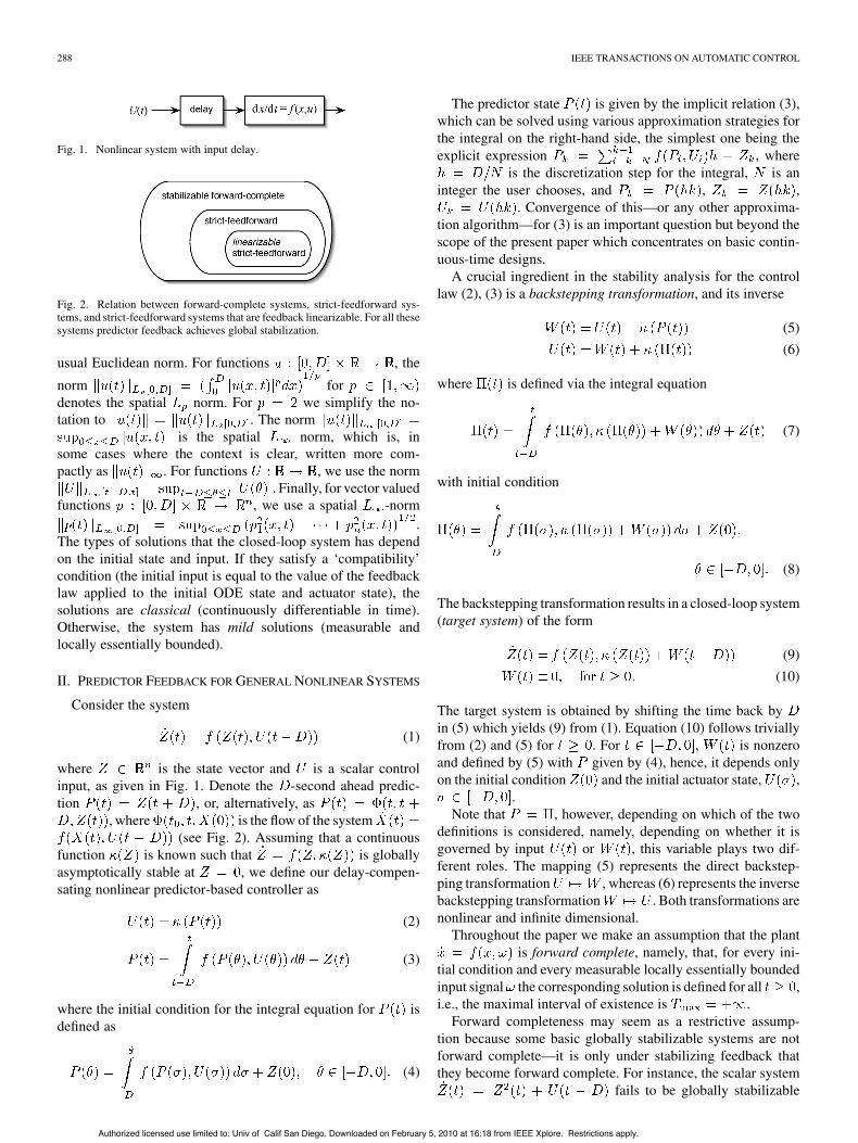
2) Contributions: With the finite escape obstacle recognized,in this paper we focus on two classes of problems for whichglobal stability is achievable in the presence of arbitrarily longinput delay. The first class is the general class of forward com-plete systems (Section VI), which do not exhibit finite escapeas long as the input remains (locally, i.e., not necessarily uni-formly) bounded. This seems like a restrictive class in a math-ematical sense, but includes most, if not all, mechanical andelectromechanical systems.

The second class is the class of strict-feedforward systems(Section VII), which is a subclass of forward complete systems.For this class, which addresses a relatively limited set of appli-cations but is important from the structural point of view, we notonly obtain global stability, but also obtain an explicit formulafor the predictor state, which is used in the nominal control lawto compensate for the input delay. This is significant, becausethe predictor state is normally not obtainable explicitly—for ex-ample, it is generally not available in explicit form for feedbacklinearizable systems.

We dedicate special attention (Section VIII) to a small butnice subclass of strict-feedforward systems which area lineariz-able by coordinate transformation [18], [51]–[53]. For thesesystems we obtain both the feedback operator and the closed-loop solutions (which are both infinite dimensional) in closedform.

3) Organization: We start in Section II where we introducea predictor-based delay compensation design for general stabi-lizable nonlinear systems. In Section V we present some impor-tant stability properties of the transport PDE in various (mostlynon-standard) norms. These technical results help in the stabilityproof for the broad class of forward-complete systems. Thenin subsequent sections we introduce a predictor feedback de-sign for general nonlinear systems and present global stabilityanalyses for the forward-complete and strict-feedforward sys-tems.

4) Notation: Several norms are used in the paper, for vec-tors and functions. For an -vector, the norm denotes the

0018-9286/$26.00 © 2010 IEEE

Authorized licensed use limited to: Univ of Calif San Diego. Downloaded on February 5, 2010 at 16:18 from IEEE Xplore. Restrictions apply.

288 IEEE TRANSACTIONS ON AUTOMATIC CONTROL

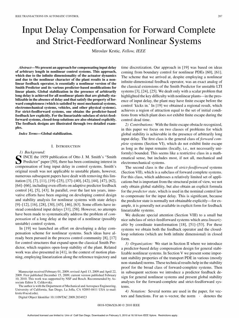
Fig. 1. Nonlinear system with input delay.

Fig. 2. Relation between forward-complete systems, strict-feedforward sys-tems, and strict-feedforward systems that are feedback linearizable. For all thesesystems predictor feedback achieves global stabilization.

usual Euclidean norm. For functions , the

norm fordenotes the spatial norm. For we simplify the no-tation to . The norm

is the spatial norm, which is, insome cases where the context is clear, written more com-pactly as . For functions , we use the norm

. Finally, for vector valuedfunctions , we use a spatial -norm

.The types of solutions that the closed-loop system has dependon the initial state and input. If they satisfy a ‘compatibility’condition (the initial input is equal to the value of the feedbacklaw applied to the initial ODE state and actuator state), thesolutions are classical (continuously differentiable in time).Otherwise, the system has mild solutions (measurable andlocally essentially bounded).

II. PREDICTOR FEEDBACK FOR GENERAL NONLINEAR SYSTEMS

Consider the system

(1)

where is the state vector and is a scalar controlinput, as given in Fig. 1. Denote the -second ahead predic-tion , or, alternatively, as

, where is the flow of the system(see Fig. 2). Assuming that a continuous

function is known such that is globallyasymptotically stable at , we define our delay-compen-sating nonlinear predictor-based controller as

(2)

(3)

where the initial condition for the integral equation for isdefined as

(4)

The predictor state is given by the implicit relation (3),which can be solved using various approximation strategies forthe integral on the right-hand side, the simplest one being theexplicit expression , where

is the discretization step for the integral, is aninteger the user chooses, and , ,

. Convergence of this—or any other approxima-tion algorithm—for (3) is an important question but beyond thescope of the present paper which concentrates on basic contin-uous-time designs.

A crucial ingredient in the stability analysis for the controllaw (2), (3) is a backstepping transformation, and its inverse

(5)

(6)

where is defined via the integral equation

(7)

with initial condition

(8)

The backstepping transformation results in a closed-loop system(target system) of the form

(9)

(10)

The target system is obtained by shifting the time back byin (5) which yields (9) from (1). Equation (10) follows triviallyfrom (2) and (5) for . For , is nonzeroand defined by (5) with given by (4), hence, it depends onlyon the initial condition and the initial actuator state, ,

.Note that , however, depending on which of the two

definitions is considered, namely, depending on whether it isgoverned by input or , this variable plays two dif-ferent roles. The mapping (5) represents the direct backstep-ping transformation , whereas (6) represents the inversebackstepping transformation . Both transformations arenonlinear and infinite dimensional.

Throughout the paper we make an assumption that the plantis forward complete, namely, that, for every ini-

tial condition and every measurable locally essentially boundedinput signal the corresponding solution is defined for all ,i.e., the maximal interval of existence is .

Forward completeness may seem as a restrictive assump-tion because some basic globally stabilizable systems are notforward complete—it is only under stabilizing feedback thatthey become forward complete. For instance, the scalar system

fails to be globally stabilizable


KRSTIC: INPUT DELAY COMPENSATION 289

for because it can exhibit finite escape for .In [19] we estimated its region of attraction under predictorfeedback. Unfortunately, many systems within popular classessuch as feedback linearizable systems, or strict-feedback sys-tems , ,

, are not globally stabilizable for becausethey are not forward complete. Hence, we look among for-ward-complete systems to find globally stabilizable nonlinearsystems with long input delay. However, we note that Hypoth-esis (A2) in [16] allows to study some strict-feedback systemsin the framework developed in the present paper.

The plant-predictor system (3) and the target-predictorsystem (7) play crucial roles in determining whether aclosed-loop system under predictor feedback is globallystable or not. If the plant is forward-complete, the plant-pre-dictor system is globally well defined, and so is the directbackstepping transformation . If theplant is globally stabilizable, then the target-predictor systemis globally well defined, and so is the inverse backsteppingtransformation .

For global stabilization via predictor feedback we require allof the following three ingredients:

1) target system is globally asymptotically stable;2) direct backstepping transformation is globally well de-

fined;3) inverse backstepping transformation is globally well de-

fined.The ingredients 1 and 3 are automatically satisfied by the ex-

istence of a globally stabilizing feedback in the absence of inputdelay . As for ingredient 2, this ingredient is missingfrom the scalar example in [19] which is not forward-completeand thus not globally stabilizable.

To summarize our conclusions, which at this point are notsupposed to be obvious but should be helpful in guiding thereader through the coming sections:

• For general systems that are globally stabilizable in the ab-sence of input delay, including feedback linearizable sys-tems and systems in the strict-feedback form, the target-predictor system and the inverse backstepping transforma-tion will be globally well defined, but this is not necessarilythe case for the plant-predictor system and the direct back-stepping transformation. Consequently, predictor feedbackwill not be globally (but only regionally) stabilizing withinthis broad class of systems.

• For forward-complete systems that are globally stabiliz-able in the absence of input delay, both the plant-predictorand the target-predictor systems, and both the direct and in-verse backstepping transformations, will be globally welldefined. Consequently, predictor feedback will be glob-ally stabilizing within this class, including its subclass ofstrict-feedforward systems.

III. STABILITY PROOF WITHOUT A LYAPUNOV FUNCTION

FOR FORWARD COMPLETE SYSTEMS

The property of predictor feedback that it exactly compen-sates the input delay, and that after seconds the closed-loopsystem evolves as if no delay were present, allows to prove sta-bility without using Lyapunov functions. This approach would

not be possible in the presence of even the most innocuous mod-eling uncertainties such as disturbances. For this reason, in Sec-tion VI we revisit the problem of stability proof using Lyapunovfunctions.

Theorem 1: Consider the closed-loop system (1), (2), (3),(4) with , and with an initial condition

and . Letbe forward complete and be globally asymp-totically stable at . Then there exists a functionsuch that

(11)

for all and for all .Proof: From the forward completeness of

, from [15, Lemma 3.5], using the fact thatwhich allows to set , we get that

, with acontinuous positive-valued monotonically increasing func-tion and a function in class . It follows that

for all. Using the fact that

for all , and using the fact that is globallyasymptotically stable at the origin, there exists a classfunction such that for all .It follows that:

(12)

for all , where we have used the fact thatfor all . Due to continuity of , there ex-ists such that . With theabove expressions we get

for all, which also implies that

forall . Now we turn our attention to estimating

over . We split the intervalin the following manner:

(13)



where . Let us now consider thefunction

.(14)

Since is a class function and are class , thereexists a class function such that for all

. For example, the function can be chosen as

.(15)

Hence,for all . Adding now

the bound (12), we get

for all . Denoting, we complete

the proof of the theorem.

IV. A TRANSPORT PDE REPRESENTATION OF THE

INFINITE-DIMENSIONAL BACKSTEPPING TRANSFORMATION

To develop Lyapunov-based tools for studying stability ofnonlinear predictor feedback, we introduce a transport PDE for-malism for representing the actuator state. We represent theplant as

(16)

(17)

(18)

and the target system as

(19)

(20)

(21)

The predictor variables are represented by the following integralequations:

(22)

(23)

where . It should be noted that, in the(22) and (23), acts as a parameter. It is helpful not to view inits role as a time variable when thinking about solutions of thesetwo nonlinear integral equations. The alternative form of theseintegral equations is as differential equations, with appropriateinitial conditions, given as

(24)

(25)

where we reiterate that these are equations in only one indepen-dent variable, , so they are not PDEs but ODEs, despite our useof partial derivative notation. The variables andare used to define the backstepping transformations (direct andinverse) as

(26)

(27)

with .Lemma 2: The functions satisfy the (16),

(17) if and only if the functions satisfy the (19),(20), where the three functions are relatedthrough (22)–(27).

Proof: This result is immediate by noting thatand are functions of only one variable, ,and therefore so are and based on theODEs (24), (25). This implies thatand , from which it follows that

and

, which completes the proof.The variables and are used to generate the

plant-predictor state and the target predictorstate . From (26) and (21) the backstepping con-trol law is given by .

V. LYAPUNOV FUNCTIONS FOR THE TRANSPORT PDE

In order to be able to construct Lypunov functions for theclosed-loop nonlinear system under predictor feedback, we needvarious Lyapunov functions for the target system’s transportPDE subsystem

(28)

(29)

where denotes its initial condition.The following results on stability and Lyapunov functions for

this system will be useful in this paper.Theorem 3: Consider the functional

, where is the classicalsolution of the system (28), (29), is any positive constant, and

is any function in class . Then, for all

(30)

(31)

Proof: The derivative of is



(32)

which yields (30). Hence, we get .Next, we observe that

. Combining the last two inequali-ties, we obtain (31).

Taking and for , , we obtain thefollowing corollary.

Corollary 4: The following holds for the system (28), (29):

(33)

for any and any .This corollary does not cover the case , which we are

also interested in. This result is proved separately.Theorem 5: Consider the functional

, where is the classicalsolution of the system (28), (29), and is any positive constant.Then, for all

(34)

(35)

Proof: Let denote the following “spatiallyweighted norm:”

(36)

where is a positive integer. Then the derivative of is givenby

(37)

With integration by parts we get

(38)



which yields (34) and finally . Then one gets(35) as follows:

(39)

The following Lyapunov fact follows from Theorem 5.Lemma 6: For any with and any ,

the derivative of the functionalong the classical solutions of the system (28), (29) is givenby .

VI. STABILITY ANALYSIS FOR FORWARD-COMPLETE

NONLINEAR SYSTEMS

The stability proof in Section III does not employ Lyapunovfunctionals but exploits properties of exact solutions to theclosed-loop system. The absence of a Lyapunov functionalwould prevent a study of stability in the presence of distur-bances and other uncertainties. Availability of a Lyapunovfunction is also important if one wants to conduct an inverseoptimal re-design of the feedback law. In this section weconstruct a Lyapunov functional for the system and conducta proof of global stability on the basis of this functional. ALypunov construction requires that we somewhat strengthen theassumptions of forward completeness and global stabilizability.

Definition 6.1: System with isstrongly forward complete if there exists a smooth function

and class functions such that

(40)

(41)

for all and for all .This property differs from standard forward completeness [1]

in the sense that we assume that and, in accordancewith that, also assume that the function is positive definite.

Assumption 6.1: The system is strongly for-ward complete.

Assumption 6.2: The system is input-to-state stable.

Before we proceed to our Lyapunov construction, we state abound on the norm of the plant-predictor system.

Lemma 7: Let system (24) satisfy Assumption 6.1. There ex-ists a function such that

(42)

Proof: With the Lyapunov-like function we getthat

(43)from which it follows that:

(44)

Using (40), we get that, which yields

. Withstandard properties of class functions, we get the result ofthe lemma.

The next two lemmas relate the norms of the plant and of thetarget system.

Lemma 8: Let system (24) satisfy Assumption 6.1 and con-sider (26) as its output map. Then there exists a function

such that

(45)Proof: With , (26), and Lemma 7.

Lemma 9: Let system (25) satisfy Assumption 6.2 and con-sider (27) as its output map. Then there exists a function

such that

(46)Proof: Under Assumption 6.2, there ex-

ists and such that

. Taking a supremum ofboth sides in , we get that

. With and(27) we obtain the result of the lemma.

Now we turn out attention to the full target system (19)–(21).Based on Assumption 6.2, there exists a smooth function

and class functions such that

(47)

(48)

for all and for all . Suppose that isa class function, or has been appropriately majorized sothis is true (with no generality lost). Take a Lyapunov function

(49)

where . This Lyapunov function is positive definite andradially unbounded (due to the assumption on ). With it weget the following result on stability in the norm of the targetsystem.

Lemma 10: Let system (19)–(21) satisfy Assumption 6.2.There exists a function such that

(50)Proof: From Lemma 6 we get that



(51)

It follows, with the help of (47), that there exists so thatand then there exists a class function

such that for all . With ad-ditional routine class calculations, using the definition (51),one can show that there exists a function such that

. From (39)we get and

. Hence,, with which we arrive

at the result of the lemma.By combining Lemmas 8, 9, and 10, we get that

. Tosummarize we obtain the following main result on closed-loopstability under predictor feedback in terms of the system normof the original plant.

Theorem 11: Let system (19)–(21) satisfy Assumptions 6.1and 6.2. Then there exists a function such that

(52)A slightly different and relevant way to state the same global

asymptotic stability result is as follows.Corollary 12: Let system (19)–(21) satisfy Assumptions 6.1

and 6.2. Then

(53)The norm on the delay state used in Theorem 11 and

Corollary 12 is a somewhat nonstandard norm in thedelay system literature. Stability in the sense of othernorms also holds. To see this, take a Lyapunov func-tional , where

and . With the help of (30) and (48),its derivative is

. With some routine classmajorizations, the following result is obtained.Theorem 13: Let system (19)–(21) satisfy Assumptions

6.1 and 6.2. Then, for any class function suchthat for all , there exists a func-tion such that

.Note that allows a significant degree of freedom in terms

of relative (functional) weighting of the ODE state and the ac-tuator state, however, this extra freedom is ‘paid for’ through

.The following example illustrates the nonlinear predictor

feedback for a system that is forward complete.Example 6.1: Consider the system ,

, which is motivated by the pendulumproblem with torque control (one can view as the angle rela-tive to the upward equilibrium, and as the angular velocity).

A predictor-based feedback law for stabilization at the originis given by ,

,, with an appropriate initial condition on . The closed-

loop system can be shown to be globally exponentially stable in

terms of the norm by em-ploying quadratic choices for .

VII. STRICT-FEEDFORWARD SYSTEMS

We now focus on a special subclass of the class of for-ward-complete systems—the strict-feedforward systems. Thesimilarity in name is pure coincidence. For forward-completesystems, the forward refers to the direction of time. Suchsystems have finite solutions for all finite positive time. Withfeedforward systems, the word forward refers to the absence offeedback in the structure of the system. The system consists ofa particular cascade of scalar systems.

Feedforward systems have received a large amount of at-tention since the early 1990s, starting with the introduction ofthis class and the first feedback laws in Teel’s thesis [54], fol-lowed by the subsequent developments by Praly and Mazenc[33] and Jankovic, Sepulchre, and Kokotovic [13], and contin-uing with extensions and generalizations by many authors [2],[6], [11], [12], [14], [18], [26]–[29], [31], [32], [34]–[36], [48],[49], [51]–[53], [56], [57], [59].

While forward complete systems yield global stability whenpredictor feedback is applied to them, the strict-feedforwardsystems have an additional property that, despite being non-linear, they can be solved explicitly. The consequence of this isthat the predictor state can be defined explicitly. Related to this,the direct infinite-dimensional backstepping transformation canbe explicitly constructed.

A special subclass of strict-feedforward systems exists, whichare linearizable by coordinate change (Section VIII). For thesesystems, not only is the predictor state explicitly defined, but theclosed-loop solutions can be found explicitly.

We introduce these ideas first through an example.

A. Example: A Second-Order Strict-Feedforward NonlinearSystem

Consider the second order system(54)

This system is the simplest ‘interesting’ example of a strict-feedforward system. The nominal controller is

(55)

and it results in the closed loop system ,, where is defined by the diffeomorphic trans-

formation(56)

The predictor is found by solving explicitly the non-linear ODE ,

with initial conditions, . The control is given by

(57)



where and are given by

(58)

(59)

The control law is a nonlinear infinite-dimensional operator, butit is given explicitly. The backstepping transformation is alsogiven explicitly

(60)

(61)

(62)

Now we derive the inverse transformation. Thistransformation is given by

, where andare the solutions of the ODE

,,

with initial condition , . It ishard to imagine that one could solve these ODEs forand directly. Indeed, for the general strict-feedbackclass, the -system won’t be solvable explicitly.

However, the present example is in the special subclass of lin-earizable strict-feedforward systems. Specifically, with a changeof variable

(63)

the plant (54), can be converted into

(64)

Then the inverse backstepping transformation is given by

(65)

where the functions and are defined through theODE ,

with initial conditions, . This ODE is

linear and we will solve it explicitly. For this, we need the matrix

exponential . With the

help of this matrix exponential, we find the solution

(66)

(67)

with which we obtain an explicit definition of the inverse back-stepping transformation (65). Like the direct one, this transfor-mation is nonlinear and infinite-dimensional.

To summarize, for the example nonlinear plant(54), we have obtained both the transformation

and its inverseexplicitly.

Now we discuss the target system given by, , ,

, where the variables are defined as in (56).This target system is a cascade of the exponentially stable trans-port PDE for and the linear exponentially stable ODE for

, which allows us to establish the following stability resultfor the closed-loop system.

Proposition 14: Consider the plant (54), in closed loop withthe controller (57)–(59). Its equilibrium at the origin

is globally asymptotically stable and locally exponentiallystable in terms of the norm

(68)

Proof: We first perform a stability analysis of thesystem using a standard Lyapunov functional as in [23], ob-taining a stability estimate in terms of the norm

(69)

Then, we turn to the direct backstepping transformation(60)–(62) and to the forwarding transformation (56) to obtaina bound on the initial value of the norm (68) in terms of theinitial value of the norm (69). Note that the relation betweenthese norms would be nonlinear. Finally, we invoke the directbackstepping transformation (65) with (66), (67), as well as the



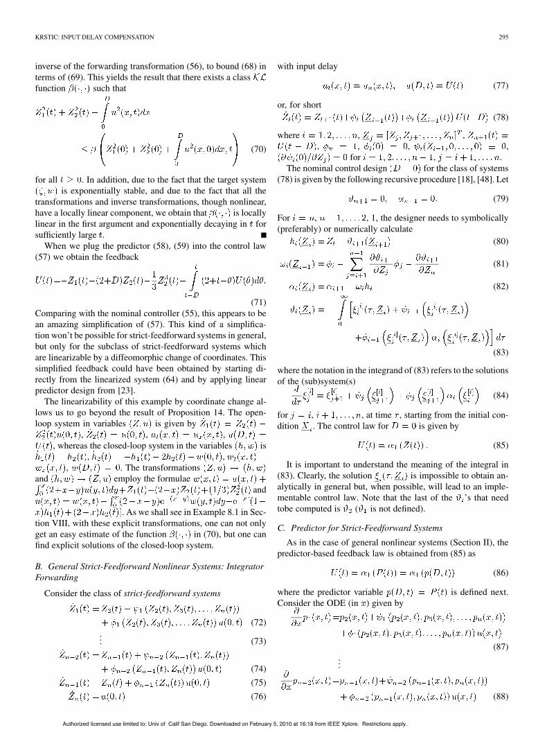
inverse of the forwarding transformation (56), to bound (68) interms of (69). This yields the result that there exists a classfunction such that

(70)

for all . In addition, due to the fact that the target systemis exponentially stable, and due to the fact that all the

transformations and inverse transformations, though nonlinear,have a locally linear component, we obtain that is locallylinear in the first argument and exponentially decaying in forsufficiently large .

When we plug the predictor (58), (59) into the control law(57) we obtain the feedback

(71)Comparing with the nominal controller (55), this appears to bean amazing simplification of (57). This kind of a simplifica-tion won’t be possible for strict-feedforward systems in general,but only for the subclass of strict-feedforward systems whichare linearizable by a diffeomorphic change of coordinates. Thissimplified feedback could have been obtained by starting di-rectly from the linearized system (64) and by applying linearpredictor design from [23].

The linearizability of this example by coordinate change al-lows us to go beyond the result of Proposition 14. The open-loop system in variables is given by

, , ,, whereas the closed-loop system in the variables is

, ,, . The transformations

and employ the formulaeand

. As we shall see in Example 8.1 in Sec-tion VIII, with these explicit transformations, one can not onlyget an easy estimate of the function in (70), but one canfind explicit solutions of the closed-loop system.

B. General Strict-Feedforward Nonlinear Systems: IntegratorForwarding

Consider the class of strict-feedforward systems

(72)... (73)

(74)

(75)

(76)

with input delay

(77)

or, for short(78)

where , ,, , , ,

for , .The nominal control design for the class of systems

(78) is given by the following recursive procedure [18], [48]. Let

(79)

For , , 1, the designer needs to symbolically(preferably) or numerically calculate

(80)

(81)

(82)

(83)

where the notation in the integrand of (83) refers to the solutionsof the (sub)system(s)

(84)

for , , at time , starting from the initial con-dition . The control law for is given by

(85)

It is important to understand the meaning of the integral in(83). Clearly, the solution is impossible to obtain an-alytically in general but, when possible, will lead to an imple-mentable control law. Note that the last of the ’s that needtobe computed is ( is not defined).

C. Predictor for Strict-Feedforward Systems

As in the case of general nonlinear systems (Section II), thepredictor-based feedback law is obtained from (85) as

(86)

where the predictor variable is defined next.Consider the ODE (in ) given by

(87)...

(88)



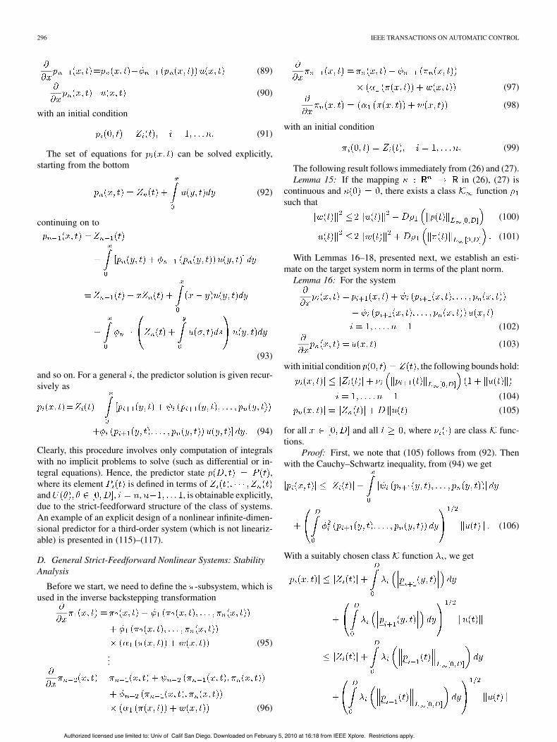
(89)

(90)

with an initial condition

(91)

The set of equations for can be solved explicitly,starting from the bottom

(92)

continuing on to

(93)

and so on. For a general , the predictor solution is given recur-sively as

(94)

Clearly, this procedure involves only computation of integralswith no implicit problems to solve (such as differential or in-tegral equations). Hence, the predictor state ,where its element is defined in terms ofand , , , is obtainable explicitly,due to the strict-feedforward structure of the class of systems.An example of an explicit design of a nonlinear infinite-dimen-sional predictor for a third-order system (which is not lineariz-able) is presented in (115)–(117).

D. General Strict-Feedforward Nonlinear Systems: StabilityAnalysis

Before we start, we need to define the -subsystem, which isused in the inverse backstepping transformation

(95)...

(96)

(97)

(98)

with an initial condition

(99)

The following result follows immediately from (26) and (27).Lemma 15: If the mapping in (26), (27) is

continuous and , there exists a class functionsuch that

(100)

(101)

With Lemmas 16–18, presented next, we establish an esti-mate on the target system norm in terms of the plant norm.

Lemma 16: For the system

(102)

(103)

with initial condition , the following bounds hold:

(104)

(105)

for all and all , where are class func-tions.

Proof: First, we note that (105) follows from (92). Thenwith the Cauchy–Schwartz inequality, from (94) we get

(106)

With a suitably chosen class function , we get



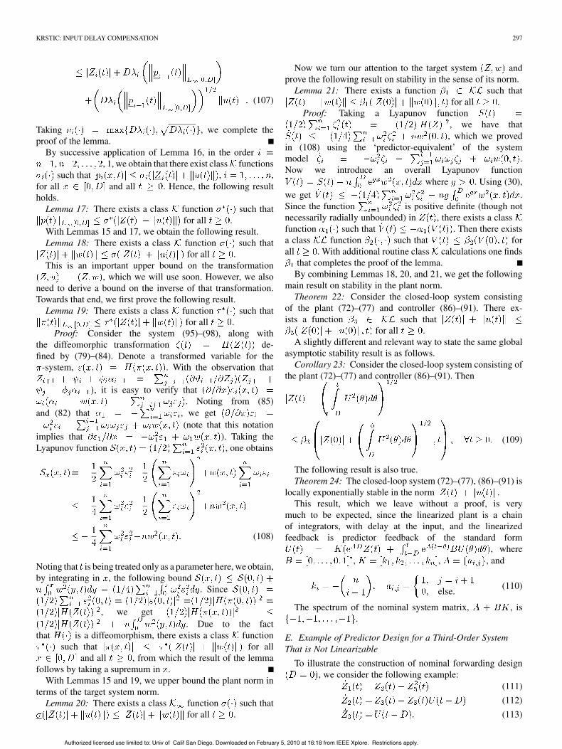
(107)

Taking , we complete theproof of the lemma.

By successive application of Lemma 16, in the order, , 1, we obtain that there exist class functionssuch that , ,

for all and all . Hence, the following resultholds.

Lemma 17: There exists a class function such thatfor all .

With Lemmas 15 and 17, we obtain the following result.Lemma 18: There exists a class function such that

for all .This is an important upper bound on the transformation

, which we will use soon. However, we alsoneed to derive a bound on the inverse of that transformation.Towards that end, we first prove the following result.


Proof: Consider the system (95)–(98), along withthe diffeomorphic transformation de-fined by (79)–(84). Denote a transformed variable for the

-system, . With the observation that

, it is easy to verify that. Noting from (85)

and (82) that , we get(note that this notation

implies that ). Taking theLyapunov function , one obtains

(108)

Noting that is being treated only as a parameter here, we obtain,by integrating in , the following bound

. Since

, we get. Due to the fact

that is a diffeomorphism, there exists a class functionsuch that for all

and all , from which the result of the lemmafollows by taking a supremum in .

With Lemmas 15 and 19, we upper bound the plant norm interms of the target system norm.


Now we turn our attention to the target system andprove the following result on stability in the sense of its norm.

Lemma 21: There exists a function such thatfor all .

Proof: Taking a Lyapunov function, we have that, which we proved

in (108) using the ‘predictor-equivalent’ of the systemmodel .Now we introduce an overall Lyapunov function

where . Using (30),we get .Since the function is positive definite (though notnecessarily radially unbounded) in , there exists a classfunction such that . Then there existsa class function such that forall . With additional routine class calculations one finds

that completes the proof of the lemma.By combining Lemmas 18, 20, and 21, we get the following

main result on stability in the plant norm.Theorem 22: Consider the closed-loop system consisting

of the plant (72)–(77) and controller (86)–(91). There ex-ists a function such that

for all .A slightly different and relevant way to state the same global

asymptotic stability result is as follows.Corollary 23: Consider the closed-loop system consisting of

the plant (72)–(77) and controller (86)–(91). Then

(109)

The following result is also true.Theorem 24: The closed-loop system (72)–(77), (86)–(91) is

locally exponentially stable in the norm .This result, which we leave without a proof, is very

much to be expected, since the linearized plant is a chainof integrators, with delay at the input, and the linearizedfeedback is predictor feedback of the standard form

, where, , , and

else. (110)

The spectrum of the nominal system matrix, , is.

E. Example of Predictor Design for a Third-Order SystemThat is Not Linearizable

To illustrate the construction of nominal forwarding design, we consider the following example:

(111)

(112)

(113)



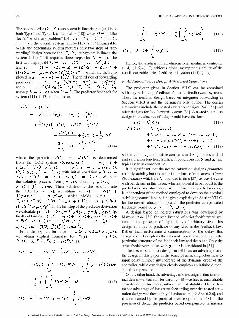
The second order subsystem is linearizable (and is ofboth Type I and Type II, as defined in [18]) when . LikeTeel’s “benchmark problem” [54], , ,

, the overall system (111)–(113) is not linearizable.While the benchmark system requires only two steps of ‘for-warding’ design because the subsystem is linear, thesystem (111)–(113) requires three steps (for ). Thefirst two steps yieldand

, which are then em-ployed in . The third step of forwardingproducesand ,namely, when . The predictor feedback forsystem (111)–(113) is obtained as

(114)

where the predictor is determinedfrom the ODE system

, ,with initial condition

, , . We startthe solution process from , obtaining

. Then, substituting this solution intothe ODE for , we obtain

, which yields

. In the last step of the predictor derivationwe calculate ,finally obtaining

.From the explicit formulae for ,

we obtain explicit formulae for ,, as

(115)

(116)

(117)

Hence, the explicit infinite-dimensional nonlinear controller(114), (115)–(117) achieves global asymptotic stability of thenon-linearizable strict-feedforward system (111)–(113).

F. An Alternative: A Design With Nested Saturations

The predictor given in Section VII-C can be combinedwith any stabilizing feedback for strict-feedforward systems.Thus, the nominal design based on integrator forwarding inSection VII-B is not the designer’s only option. The designalternatives include the nested saturation designs [54], [56] andother designs for feedforward systems [33]. A nested saturationdesign in the absence of delay would have the form

(118)

(119)

where and are positive constants and is the standardunit saturation function. Sufficient conditions for and aretypically very conservative.

It is significant that the nested saturation designs guaranteenot only stability but also a particular form of robustness to inputdisturbances which are bounded in time [57], as was the casewith our design in this paper, which allowed it to be robust to thepredictor error disturbance, . Since the predictor designis independent of the method employed to develop the nominalstabilizing controller, and it is given explicitly in Section VII-C,for the nested saturation approach, the predictor-compensatedfeedback would be .

A design based on nested saturations was developed byMazenc et al. [31] for stabilization of strict-feedforward sys-tems in the presence of input delay of arbitrary size. Thisdesign employs no predictor of any kind in the feedback law.Rather than performing a compensation of the delay, thisdesign cleverly exploits the inherent robustness to delay in theparticular structure of the feedback law and the plant. Only thestrict-feedforward class with is considered in [31].

The nested saturation design in [31] has an advantage overthe design in this paper in the sense of achieving robustness toinput delay without any increase of the dynamic order of thecontroller, while our design clearly employs an infinite-dimen-sional compensator.

On the other hand, the advantage of our design is that its nom-inal design—integrator forwarding [48]—achieves quantifiableclosed-loop performance, rather than just stability. The perfor-mance advantage of integrator forwarding over the nested satu-ration design was thoroughly illuminated in [49, Sec. 6.2.6], andit is reinforced by the proof of inverse optimality [48]. In thepresence of delay, the predictor-based compensator maintains



the performance of the nominal forwarding design, modulo thefirst seconds. Thus, a clear complexity-versus-performancetradeoff exists between the design in this paper and the designin [31].

VIII. LINEARIZABLE STRICT-FEEDFORWARD SYSTEMS

Most strict-feedforward systems are not feedback lineariz-able, however a small class of strict-feedforward systems is lin-earizable, and, in fact, it is linearizable by coordinate changealone, without the use of feedback. In this section we reviewthe conditions for linearizability of strict-feedofrward systems,present a control algorithm which results in explicit formulaefor control laws, present formulae for predictor feedbacks thatcompensate for actuator delays (which happen to be nonlinearin the ODE state but linear in the distributed actuator state), andderive the formulae for closed-loop solutions in the presence ofactuator delay.

A. Integrator Forwarding (SJK) Algorithm Applied toLinearizable Strict-Feedforward Systems

In [18] it was shown that a strict-feedforward system (withoutdelay)

(120)

is linearizable provided the following assumption is satisfied (asystematic approach to satisfying this assumption was subse-quently developed by Tall and Respondek [52], [53]).

Assumption 8.1: The functions can bewritten as , , and

(121)

(122)

for , using some scalar-valued functionssatisfying for ,

.If Assumpiton 8.1 is satisfied, then the functions are

used in the diffeomorphism(123)

(124)

for transforming the strict-feedforward system (120) into asystem of the “chain of integrators” form

(125)

(126)

The general control design algorithm for linearizable strict-feedforward systems starts with , , andcontinues recursively, for , , 1, as

(127)

(128)

(129)

(130)

(131)

The control law is .There are two sets of linearizing coordinates, one given by

, which, with the control law, yields the closed-loop system

in the “Teel form” [55]

......

. . ....

.... . .

. . .

(132)

and the other set of coordinates given by, which, with the control law

yields the closed-loop systemin the companion form

(133)

(134)

Both the -coordinates and the -coordinates have a useful pur-pose, as we shall see when we study the system in the presenceof actuator delay.

B. Predictor Feedback for Linearizable Strict-FeedforwardSystems

Now we consider the system with actuator delay

(135)

(136)

(137)

With the diffeomporphic transformation , i.e.,, which is recursively defined by and

(138)

we get the system(139)

(140)



(141)

(142)

which is a cascade of a delay line and a chain of integrators. Thepredictor feedback design for this system is easy.

Denote by the state of the system

(143)

(144)

with initial condition . The predictor feedback isgiven as

(145)Fortunately, the -system can be solved explicitly

(146)so the “predictor” is obtained as

(147)Substituting the transformation , we get thepredictor

(148)

Plugging this predictor into the predictor feedback law, we getthe feedback law explicitly

(149)

Replacing by , we finally get

(150)

This feedback law is linear in the infinite-dimensional delaystate , but nonlinear in the ODE plant state .

The infinite-dimensional backstepping transformation and itsinverse are given by

(151)

(152)

where

(153)

(154)

with initial condition .The proof of stability for the general design in this section

for linearizable strict-feedforward systems proceeds in a similarmanner as for general strict-feedforward systems, except that afew of the steps can be completed explicitly or more directly bynoting that, with the predictor feedback, the closed-loop systemin the variables is

(155)

(156)

(157)

(158)

In the end, the following result is obtained.Theorem 25: Consider the closed-loop system consisting

of the plant (135)–(137) under Assumption 8.1 and controller(150). There exists a class function such that

(159)

C. Explicit Closed-Loop Solutions for LinearizableStrict-Feedforward Systems

For linearizable strict-forward systems one can find theclosed-loop solutions. Over the time interval oneuses the linear model

(160)

(161)

whereas over the time interval one would use the model(162)

(163)

where the delay has been completely compensated.For the time period we obtain



(164)

whereas for the time period we get

(165)

where , , ,

else (166)

and

(167)

Theorem 26: Consider the closed-loop system consistingof the plant (135)–(137) under Assumption 8.1 and controller(150). The closed-loop solution is given by ,where is given by (164) for and by (165), (167)for .

Example 8.1: To illustrate this theorem, we return to the ex-ample plant (54), from Section VII-A. We will now calculatethe explicit solution for this system in closed loop with feed-back (71). For simplicity of calculations, we will assume thatthe initial actuator state is zero, namely, .Over the time interval the solution is given by

, . To find the solutionfor , we recall the linearizing transformation for this ex-ample from (63): , .The resulting equations for , ,can be solved as

(168)

(169)

Using the linearizing transformation, is obtained as, .

To find the solution for , we need the inverse of thelinearizing transformation, (63): ,

. By substituting into and then into, we obtain the closed-loop solutions explicitly as

(170)

(171)

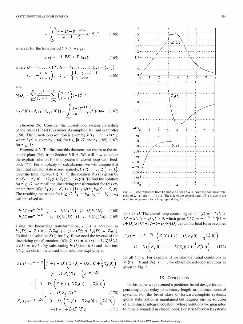
Fig. 3. Time responses from Example 8.1 for . Note the nonlinear tran-sient of after . The size of the control input is due to theneed to compensate for a long input delay, .

for . The closed-loop control signal is, which gives

, and in its final form becomes

(172)

for all . For example, if we take the initial conditions asand , we obtain closed-loop solutions as

given in Fig. 3.

IX. CONCLUSION

In this paper we presented a predictor-based design for com-pensating input delay of arbitrary length in nonlinear controlsystems. For the broad class of forward-complete systems,global stabilization is maintained but requires on-line solutionof a nonlinear integral equation (whose solutions we guaranteeto remain bounded in closed loop). For strict-feedback systems



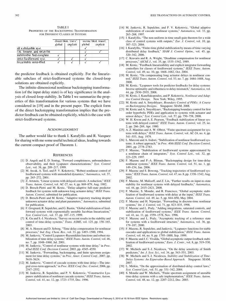
TABLE IPROPERTIES OF THE BACKSTEPPING TRANSFORMATION

FOR DIFFERENT CLASSES OF SYSTEMS

the predictor feedback is obtained explicitly. For the lineariz-able subclass of strict-feedforward systems the closed-loopsolutions are obtained explicitly.

The infinite-dimensional nonlinear backstepping transforma-tion (of the input delay state) is of key significance in the anal-ysis of closed-loop stability. In Table I we summarize the prop-erties of this transformation for various systems that we haveconsidered in [19] and in the present paper. The explicit formof the direct backstepping transformation implies that the pre-dictor feedback can be obtained explicitly, which is the case withstrict-feedforward systems.

ACKNOWLEDGMENT

The author would like to thank I. Karafyllis and R. Vazquezfor sharing with me some useful technical ideas, leading towardsthe current compact proof of Theorem 1.

REFERENCES

[1] D. Angeli and E. D. Sontag, “Forward completeness, unboundednessobservability, and their Lyapunov characterizations,” Syst. ControlLett., vol. 38, pp. 209–217, 1999.

[2] M. Arcak, A. Teel, and P. V. Kokotovic, “Robust nonlinear control offeedforward systems with unmodeled dynamics,” Automatica, vol. 37,pp. 265–272, 2001.

[3] Z. Artstein, “Linear systems with delayed controls: A reduction,” IEEETrans. Autom. Control, vol. AC-27, no. 4, pp. 869–879, Aug. 1982.

[4] D. Bresch-Pietri and M. Krstic, “Delay-adaptive full-state predictorfeedback for systems with unknown long actuator delay,” IEEE Trans.Autom. Control, submitted for publication.

[5] D. Bresch-Pietri and M. Krstic, “Adaptive trajectory tracking despiteunknown actuator delay and plant parameters,” Automatica, submittedfor publication.

[6] F. Grognard, R. Sepulchre, and G. Bastin, “Global stabilization of feed-forward systems with exponentially unstable Jacobian linearization,”Syst. Control Lett., vol. 37, pp. 107–115, 1999.

[7] K. Gu and S.-I. Niculescu, “Survey on recent results in the stability andcontrol of time-delay systems,” Trans. ASME, vol. 125, pp. 158–165,2003.

[8] M. A. Henson and D. Seborg, “Time delay compensation for nonlinearprocesses,” Ind. Eng. Chem. Res., vol. 33, pp. 1493–1500, 1994.

[9] M. Jankovic, “Control Lyapunov-Razumikhin functions and robust sta-bilization of time delay systems,” IEEE Trans. Autom. Control, vol. 46,no. 7, pp. 1048–1060, Jul. 2001.

[10] M. Jankovic, “Control of nonlinear systems with time delay,” in Proc.42nd IEEE Conf. Decision Control, 2003, pp. 4545–4550.

[11] M. Jankovic, “Forwarding, backstepping, and finite spectrum assign-ment for time delay systems,” in Proc. Amer. Control Conf., 2007, pp.5618–5624.

[12] M. Jankovic, “Control of cascade systems with time delay—The inte-gral cross-term approach,” in Proc. IEEE Conf. Dec. Control, 2006, pp.2547–2552.

[13] M. Jankovic, R. Sepulchre, and P. V. Kokotovic, “Constructive Lya-punov stabilization of nonlinear cascade systems,” IEEE Trans. Autom.Control, vol. 41, no. 12, pp. 1723–1735, Dec. 1996.

[14] M. Jankovic, R. Sepulchre, and P. V. Kokotovic, “Global adaptivestabilization of cascade nonlinear systems,” Automatica, vol. 33, pp.263–268, 1997.

[15] I. Karafyllis, “The non-uniform in time small-gain theorem for a wideclass of control systems with outputs,” Eur. J. Control, vol. 10, pp.307–323, 2004.

[16] I. Karafyllis, “Finite-time global stabilization by means of time-varyingdistributed delay feedback,” SIAM J. Control Optim., vol. 45, pp.320–342, 2006.

[17] C. Kravaris and R. A. Wright, “Deadtime compensation for nonlinearprocesses,” AIChE J., vol. 35, pp. 1535–1542, 1989.

[18] M. Krstic, “Feedback linearizability and explicit integrator forwardingcontrollers for classes of feedforward systems,” IEEE Trans. Autom.Control, vol. 49, no. 10, pp. 1668–1682, Oct. 2004.

[19] M. Krstic, “On compensating long actuator delays in nonlinear con-trol,” IEEE Trans. Autom. Control, vol. 53, no. 7, pp. 1684–1688, Aug.2008.

[20] M. Krstic, “Lyapunov tools for predictor feedbacks for delay systems:Inverse optimality and robustness to delay mismatch,” Automatica, vol.44, pp. 2930–2935, 2008.

[21] M. Krstic, I. Kanellakopoulos, and P. Kokotovic, Nonlinear and Adap-tive Control Design. New York: Wiley, 1995.

[22] M. Krstic and A. Smyshlyaev, Boundary Control of PDEs: A Courseon Backstepping Designs. Singapore: SIAM, 2008.

[23] M. Krstic and A. Smyshlyaev, “Backstepping boundary control for firstorder hyperbolic PDEs and application to systems with actuator andsensor delays,” Syst. Control Lett., vol. 57, pp. 750–758, 2008.

[24] W. H. Kwon and A. E. Pearson, “Feedback stabilization of linear sys-tems with delayed control,” IEEE Trans. Autom. Control, vol. 25, no.2, pp. 266–269, Apr. 1980.

[25] A. Z. Manitius and A. W. Olbrot, “Finite spectrum assignment for sys-tems with delays,” IEEE Trans. Autom. Control, vol. AC-24, no. 4, pp.541–553, Aug. 1979.

[26] L. Marconi and A. Isidori, “Stabilization of nonlinear feedforward sys-tems: A robust approach,” in Proc. 40th IEEE Conf. Decision Control,2001, pp. 2778–2783.

[27] F. Mazenc, “Stabilization of feedforward systems approximated bya nonlinear chain of integrators,” Syst. Control Lett., vol. 32, pp.223–229, 1997.

[28] F. Mazenc and P.-A. Bliman, “Backstepping design for time-delaynonlinear systems,” IEEE Trans. Autom. Control, vol. 51, no. 1, pp.149–154, Jan. 2006.

[29] F. Mazenc and S. Bowong, “Tracking trajectories of feedforward sys-tems,” IEEE Trans. Autom. Control, vol. 47, no. 8, pp. 1338–1342, Aug.2002.

[30] F. Mazenc, M. Malisoff, and Z. Lin, “Further results on input-to-statestability for nonlinear systems with delayed feedbacks,” Automatica,vol. 44, pp. 2415–2421, 2008.

[31] F. Mazenc, S. Mondie, and R. Francisco, “Global asymptotic stabi-lization of feedforward systems with delay at the input,” IEEE Trans.Autom. Control, vol. 49, no. 5, pp. 844–850, May 2004.

[32] F. Mazenc and H. Nijmeijer, “Forwarding in discrete-time nonlinearsystems,” Int. J. Control, vol. 71, pp. 823–835, 1998.

[33] F. Mazenc and L. Praly, “Adding integrations, saturated controls, andstabilization of feedforward systems,” IEEE Trans. Autom. Control,vol. 41, no. 11, pp. 1559–1578, Nov. 1996.

[34] F. Mazenc and L. Praly, “Asymptotic tracking of a reference statefor systems with a feedforward structure,” Automatica, vol. 36, pp.179–187, 2000.

[35] F. Mazenc, R. Sepulchre, and Jankovic, “Lyapunov functions for stablecascades and applications to global stabilization,” IEEE Trans. Autom.Control, vol. 44, no. 9, pp. 1795–1800, Sep. 1999.

[36] F. Mazenc and J. C. Vivalda, “Global asymptotic output feedback stabi-lization of feedforward systems,” Euro. J. Contr., vol. 8, pp. 519–530,2002.

[37] W. Michiels and S.-I. Niculescu, “On the delay sensitivity of Smithpredictors,” Int. J. Syst. Sci., vol. 34, pp. 543–551, 2003.

[38] W. Michiels and S.-I. Niculescu, Stability and Stabilization of Time-Delay Systems: An Eignevalue-Based Approach. Singapore: SIAM,2007.

[39] L. Mirkin, “On the approximation of distributed-delay control laws,”Syst. Control Lett., vol. 51, pp. 331–342, 2004.

[40] S. Mondie and W. Michiels, “Finite spectrum assignment of unstabletime-delay systems with a safe implementation,” IEEE Trans. Autom.Control, vol. 48, no. 12, pp. 2207–2212, Dec. 2003.



[41] H. Mounier and J. Rudolph, “Flatness-based control of nonlinear delaysystems: A chemical reactor example,” Int. J. Control, vol. 71, pp.871–890, 1998.

[42] S.-I. Niculescu, Delay Effects on Stability. New York: Springer, 2001.[43] S.-I. Niculescu and A. M. Annaswamy, “An adaptive Smith-controller

for time-delay systems with relative degree ,” Syst. ControlLett., vol. 49, pp. 347–358, 2003.

[44] A. W. Olbrot, “Stabilizability, detectability, and spectrum assignmentfor linear autonomous systems with general time delays,” IEEE Trans.Autom. Control, vol. AC-23, no. 5, pp. 887–890, Oct. 1978.

[45] P. Pepe and Z.-P. Jiang, “A Lyapunov-Krasovskii methodology forISS and iISS of time-delay systems,” Syst. Control Lett., vol. 55, pp.1006–1014, 2006.

[46] P. Pepe, I. Karafyllis, and Z.-P. Jiang, “On the Liapunov-Krasovskiimethodology for the ISS of systems described by coupled delay differ-ential and difference equations,” Automatica, vol. 44, pp. 2266–2273,2008.

[47] J.-P. Richard, “Time-delay systems: An overview of some recent ad-vances and open problems,” Automatica, vol. 39, pp. 1667–1694, 2003.

[48] R. Sepulchre, M. Jankovic, and P. V. Kokotovic, “Integrator for-warding: A new recursive nonlinear robust design,” Automatica, vol.33, pp. 979–984, 1997.

[49] R. Sepulchre, M. Jankovic, and P. Kokotovic, Constructive NonlinearControl. New York: Springer, 1997.

[50] O. J. M. Smith, “A controller to overcome dead time,” ISA, vol. 6, pp.28–33, 1959.

[51] I. A. Tall and W. Respondek, “Transforming a single-input nonlinearsystem to a feedforward form via feedback,” in Nonlinear Control inthe Year 2000, A. Isidori, F. Lamnabhi-Lagarrigue, and W. Respondek,Eds. New York: Springer, 2000, vol. 259, LNCIS, pp. 527–542, vol.2.

[52] I. A. Tall and W. Respondek, “On linearizability of strict feedforwardsystems,” in Proc. Amer. Control Conf., Seattle, WA, 2008, pp.1929–1934.

[53] I. A. Tall and W. Respondek, “Feedback linearizable strict feedforwardsystems,” in Proc. 47th IEEE Conf. Decision Control, Cancun, Mexico,2008, pp. 2499–2504.

[54] A. R. Teel, “Feedback Stabilization: Nonlinear Solutions to InherentlyNonlinear Problems,” PhD dissertation, Univ. California, Berkeley,1992.

[55] A. R. Teel, “Global stabilization and restricted tracking for multipleintegrators with bounded controls,” Syst. Control Lett., vol. 18, pp.165–171, 1992.

[56] A. R. Teel, “A nonlinear small gain theorem for the analysis of controlsystems with saturation,” IEEE Trans. Autom. Control, vol. 41, no. 9,pp. 1256–1270, Sep. 1996.

[57] A. R. Teel, “On performance induced by feedbacks with multiplesaturations,” ESAIM: Control, Optim., Calculus Variations, vol. 1, pp.225–240, 1996.

[58] A. R. Teel, “Connections between Razumikhin-type theorems and theISS nonlinear small gain theorem,” IEEE Trans. Autom. Control, vol.43, no. 7, pp. 960–964, Jul. 1998.

[59] J. Tsinias and M. P. Tzamtzi, “An explicit formula of bounded feedbackstabilizers for feedforward systems,” Syst. Control Lett., vol. 43, pp.247–261, 2001.

[60] R. Vazquez and M. Krstic, “Control of 1-D parabolic PDEs withVolterra nonlinearities—Part I: Design,” Automatica, to be published.

[61] R. Vazquez and M. Krstic, “Control of 1-D parabolic PDEs withVolterra nonlinearities—Part II: Analysis,” Automatica, to be pub-lished.

[62] K. Watanabe, “Finite spectrum assignment and observer for multivari-able systems with commensurate delays,” IEEE Trans. Autom. Control,vol. 31, no. 6, pp. 543–550, Jun. 1996.

[63] N. Yeganefar, P. Pepe, and M. Dambrine, “Input-to-state stability oftime-delay systems: A link with exponential stability,” IEEE Trans.Autom. Control, vol. 53, no. 6, pp. 1526–1531, Jul. 2008.

[64] Q.-C. Zhong, “On distributed delay in linear control laws—Part I: Dis-crete-delay implementation,” IEEE Trans. Autom. Control, vol. 49, no.11, pp. 2074–2080, Nov. 2004.

[65] Q.-C. Zhong, Robust Control of Time-Delay Systems. New York:Springer, 2006.

[66] Q.-C. Zhong and L. Mirkin, “Control of integral processes with deadtime—Part 2: Quantitative analysis,” Proc. Inst. Elect. Eng., vol. 149,pp. 291–296, 2002.

Miroslav Krstic (S’92–M’95–SM’99–F’02) re-ceived the Ph.D. degree from the University ofCalifornia, Santa Barbara, in 1994.

He was an Assistant Professor at the Universityof Maryland, College Park, until 1997. He is theSorenson Distinguished Professor and the foundingDirector of the Cymer Center for Control Systemsand Dynamics (CCSD) at UC San Diego. He is acoauthor of eight books: Nonlinear and AdaptiveControl Design (New York: Wiley, 1995), Sta-bilization of Nonlinear Uncertain Systems (New

York: Springer, 1998), Flow Control by Feedback (New York: Springer,2002), Real-time Optimization by Extremum Seeking Control (New York:Wiley, 2003), Control of Turbulent and Magnetohydrodynamic Channel Flows(Boston, MA: Birkhauser, 2007), Boundary Control of PDEs: A Course onBackstepping Designs (Singapore: SIAM, 2008), Delay Compensation forNonlinear, Adaptive, and PDE Systems (Boston, MA: Birkhauser, 2009), andAdaptive Control of Parabolic PDEs (Princeton, NJ: Princeton Univ. Press,2009).

Dr. Krstic is a Fellow of IFAC and has received the Axelby and Schuck PaperPrizes, NSF Career, ONR Young Investigator, and PECASE Award. He has heldthe appointment of Springer Distinguished Visiting Professor of Mechanical En-gineering at UC Berkeley.


ieee transactions on automatic control 287 …flyingv.ucsd.edu/papers/pdf/121.pdf · input delay...

Documents