ieee recommended practice for excitation system...
TRANSCRIPT

IEEE Recommended Practice for Excitation System Models for Power System Stability Studies
Sponsored by the Energy Development and Power Generation Committee
IEEE 3 Park Avenue New York, NY 10016-5997 USA
IEEE Power and Energy Society
IEEE Std 421.5™-2016 (Revision of
IEEE Std 421.5-2005)
Authorized licensed use limited to: Iowa State University. Downloaded on January 07,2018 at 21:03:12 UTC from IEEE Xplore. Restrictions apply.

IEEE Std 421.5™-2016 (Revision of
IEEE Std 421.5-2005)
IEEE Recommended Practice for Excitation System Models for Power System Stability Studies
Sponsor Energy Development and Power Generation Committee of the IEEE Power and Energy Society Approved 15 May 2016 IEEE-SA Standards Board
Authorized licensed use limited to: Iowa State University. Downloaded on January 07,2018 at 21:03:12 UTC from IEEE Xplore. Restrictions apply.

Abstract: Excitation system and power system stabilizer models suitable for use in large-scale system stability studies are presented. Important excitation limiters and supplementary controls are also included. The model structures presented are intended to facilitate the use of field test data as a means of obtaining model parameters. The models are, however, reduced order models and do not necessarily represent all of the control loops of any particular system. The models are valid for frequency deviations of ±5% from rated frequency and oscillation frequencies up to 3 Hz. These models would not normally be adequate for use in studies of subsynchronous resonance or other shaft torsional interaction behavior. Delayed protective and control features that may come into play in long-term dynamic performance studies are not represented. A sample set of data for each of the models, for at least one particular application, is provided. Keywords: excitation limiter models, excitation systems models, IEEE 421.5™, power system stability, power system stabilizer models
•
The Institute of Electrical and Electronics Engineers, Inc. 3 Park Avenue, New York, NY 10016-5997, USA Copyright © 2016 by The Institute of Electrical and Electronics Engineers, Inc. All rights reserved. Published 26 August 2016. Printed in the United States of America. IEEE is a registered trademark in the U.S. Patent & Trademark Office, owned by The Institute of Electrical and Electronics Engineers, Incorporated. PDF: ISBN 978-1-5044-0855-4 STD20896 Print: ISBN 978-1-5044-0856-1 STDPD20896 IEEE prohibits discrimination, harassment, and bullying. For more information, visit http://www.ieee.org/web/aboutus/whatis/policies/p9-26.html. No part of this publication may be reproduced in any form, in an electronic retrieval system or otherwise, without the prior written permission of the publisher.
Copyright © 2016 IEEE. All rights reserved.
ii
Authorized licensed use limited to: Iowa State University. Downloaded on January 07,2018 at 21:03:12 UTC from IEEE Xplore. Restrictions apply.

Important Notices and Disclaimers Concerning IEEE Standards Documents
IEEE documents are made available for use subject to important notices and legal disclaimers. These notices and disclaimers, or a reference to this page, appear in all standards and may be found under the heading “Important Notice” or “Important Notices and Disclaimers Concerning IEEE Standards Documents.”
Notice and Disclaimer of Liability Concerning the Use of IEEE Standards Documents
IEEE Standards documents (standards, recommended practices, and guides), both full-use and trial-use, are developed within IEEE Societies and the Standards Coordinating Committees of the IEEE Standards Association (“IEEE-SA”) Standards Board. IEEE (“the Institute”) develops its standards through a consensus development process, approved by the American National Standards Institute (“ANSI”), which brings together volunteers representing varied viewpoints and interests to achieve the final product. Volunteers are not necessarily members of the Institute and participate without compensation from IEEE. While IEEE administers the process and establishes rules to promote fairness in the consensus development process, IEEE does not independently evaluate, test, or verify the accuracy of any of the information or the soundness of any judgments contained in its standards.
IEEE does not warrant or represent the accuracy or content of the material contained in its standards, and expressly disclaims all warranties (express, implied and statutory) not included in this or any other document relating to the standard, including, but not limited to, the warranties of: merchantability; fitness for a particular purpose; non-infringement; and quality, accuracy, effectiveness, currency, or completeness of material. In addition, IEEE disclaims any and all conditions relating to: results; and workmanlike effort. IEEE standards documents are supplied “AS IS” and “WITH ALL FAULTS.”
Use of an IEEE standard is wholly voluntary. The existence of an IEEE standard does not imply that there are no other ways to produce, test, measure, purchase, market, or provide other goods and services related to the scope of the IEEE standard. Furthermore, the viewpoint expressed at the time a standard is approved and issued is subject to change brought about through developments in the state of the art and comments received from users of the standard.
In publishing and making its standards available, IEEE is not suggesting or rendering professional or other services for, or on behalf of, any person or entity nor is IEEE undertaking to perform any duty owed by any other person or entity to another. Any person utilizing any IEEE Standards document, should rely upon his or her own independent judgment in the exercise of reasonable care in any given circumstances or, as appropriate, seek the advice of a competent professional in determining the appropriateness of a given IEEE standard.
IN NO EVENT SHALL IEEE BE LIABLE FOR ANY DIRECT, INDIRECT, INCIDENTAL, SPECIAL, EXEMPLARY, OR CONSEQUENTIAL DAMAGES (INCLUDING, BUT NOT LIMITED TO: PROCUREMENT OF SUBSTITUTE GOODS OR SERVICES; LOSS OF USE, DATA, OR PROFITS; OR BUSINESS INTERRUPTION) HOWEVER CAUSED AND ON ANY THEORY OF LIABILITY, WHETHER IN CONTRACT, STRICT LIABILITY, OR TORT (INCLUDING NEGLIGENCE OR OTHERWISE) ARISING IN ANY WAY OUT OF THE PUBLICATION, USE OF, OR RELIANCE UPON ANY STANDARD, EVEN IF ADVISED OF THE POSSIBILITY OF SUCH DAMAGE AND REGARDLESS OF WHETHER SUCH DAMAGE WAS FORESEEABLE.
Translations
The IEEE consensus development process involves the review of documents in English only. In the event that an IEEE standard is translated, only the English version published by IEEE should be considered the approved IEEE standard.
Copyright © 2016 IEEE. All rights reserved.
iii
Authorized licensed use limited to: Iowa State University. Downloaded on January 07,2018 at 21:03:12 UTC from IEEE Xplore. Restrictions apply.

Official statements
A statement, written or oral, that is not processed in accordance with the IEEE-SA Standards Board Operations Manual shall not be considered or inferred to be the official position of IEEE or any of its committees and shall not be considered to be, or be relied upon as, a formal position of IEEE. At lectures, symposia, seminars, or educational courses, an individual presenting information on IEEE standards shall make it clear that his or her views should be considered the personal views of that individual rather than the formal position of IEEE.
Comments on standards
Comments for revision of IEEE Standards documents are welcome from any interested party, regardless of membership affiliation with IEEE. However, IEEE does not provide consulting information or advice pertaining to IEEE Standards documents. Suggestions for changes in documents should be in the form of a proposed change of text, together with appropriate supporting comments. Since IEEE standards represent a consensus of concerned interests, it is important that any responses to comments and questions also receive the concurrence of a balance of interests. For this reason, IEEE and the members of its societies and Standards Coordinating Committees are not able to provide an instant response to comments or questions except in those cases where the matter has previously been addressed. For the same reason, IEEE does not respond to interpretation requests. Any person who would like to participate in revisions to an IEEE standard is welcome to join the relevant IEEE working group.
Comments on standards should be submitted to the following address:
Secretary, IEEE-SA Standards Board 445 Hoes Lane Piscataway, NJ 08854 USA
Laws and regulations
Users of IEEE Standards documents should consult all applicable laws and regulations. Compliance with the provisions of any IEEE Standards document does not imply compliance to any applicable regulatory requirements. Implementers of the standard are responsible for observing or referring to the applicable regulatory requirements. IEEE does not, by the publication of its standards, intend to urge action that is not in compliance with applicable laws, and these documents may not be construed as doing so.
Copyrights
IEEE draft and approved standards are copyrighted by IEEE under U.S. and international copyright laws. They are made available by IEEE and are adopted for a wide variety of both public and private uses. These include both use, by reference, in laws and regulations, and use in private self-regulation, standardization, and the promotion of engineering practices and methods. By making these documents available for use and adoption by public authorities and private users, IEEE does not waive any rights in copyright to the documents.
Photocopies
Subject to payment of the appropriate fee, IEEE will grant users a limited, non-exclusive license to photocopy portions of any individual standard for company or organizational internal use or individual, non-commercial use only. To arrange for payment of licensing fees, please contact Copyright Clearance Center, Customer Service, 222 Rosewood Drive, Danvers, MA 01923 USA; +1 978 750 8400. Permission to photocopy portions of any individual standard for educational classroom use can also be obtained through the Copyright Clearance Center.
Copyright © 2016 IEEE. All rights reserved.
iv
Authorized licensed use limited to: Iowa State University. Downloaded on January 07,2018 at 21:03:12 UTC from IEEE Xplore. Restrictions apply.

Copyright © 2016 IEEE. All rights reserved.
v
Updating of IEEE Standards documents
Users of IEEE Standards documents should be aware that these documents may be superseded at any time by the issuance of new editions or may be amended from time to time through the issuance of amendments, corrigenda, or errata. An official IEEE document at any point in time consists of the current edition of the document together with any amendments, corrigenda, or errata then in effect.
Every IEEE standard is subjected to review at least every ten years. When a document is more than ten years old and has not undergone a revision process, it is reasonable to conclude that its contents, although still of some value, do not wholly reflect the present state of the art. Users are cautioned to check to determine that they have the latest edition of any IEEE standard.
In order to determine whether a given document is the current edition and whether it has been amended through the issuance of amendments, corrigenda, or errata, visit the IEEE-SA Website at http://ieeexplore.ieee.org/Xplore/ or contact IEEE at the address listed previously. For more information about the IEEE SA or IEEE’s standards development process, visit the IEEE-SA Website at http://standards.ieee.org.
Errata
Errata, if any, for all IEEE standards can be accessed on the IEEE-SA Website at the following URL: http://standards.ieee.org/findstds/errata/index.html. Users are encouraged to check this URL for errata periodically.
Patents
Attention is called to the possibility that implementation of this standard may require use of subject matter covered by patent rights. By publication of this standard, no position is taken by the IEEE with respect to the existence or validity of any patent rights in connection therewith. If a patent holder or patent applicant has filed a statement of assurance via an Accepted Letter of Assurance, then the statement is listed on the IEEE-SA Website at http://standards.ieee.org/about/sasb/patcom/patents.html. Letters of Assurance may indicate whether the Submitter is willing or unwilling to grant licenses under patent rights without compensation or under reasonable rates, with reasonable terms and conditions that are demonstrably free of any unfair discrimination to applicants desiring to obtain such licenses.
Essential Patent Claims may exist for which a Letter of Assurance has not been received. The IEEE is not responsible for identifying Essential Patent Claims for which a license may be required, for conducting inquiries into the legal validity or scope of Patents Claims, or determining whether any licensing terms or conditions provided in connection with submission of a Letter of Assurance, if any, or in any licensing agreements are reasonable or non-discriminatory. Users of this standard are expressly advised that determination of the validity of any patent rights, and the risk of infringement of such rights, is entirely their own responsibility. Further information may be obtained from the IEEE Standards Association.
Authorized licensed use limited to: Iowa State University. Downloaded on January 07,2018 at 21:03:12 UTC from IEEE Xplore. Restrictions apply.
Participants
At the time this IEEE recommended practice was completed, the Identification, Testing, and Evaluation of the Dynamic Performance of Excitation Control Systems Working Group had the following membership:
Les Hajagos, Chair Robert Thornton-Jones, Vice Chair
Leonardo Lima, Secretary
Matthias Baechle Michael Basler Michael Faltas James Feltes Namal Fernando Luc Gerin-Lajoie Alexander Glaninger-Katschnig Joseph Hurley Chavdar Ivanov
Kiyong Kim Ruediger Kutzner Eric Lambert Shawn McMullen Richard Mummert Shawn Patterson Juan Sanchez-Gasca Richard Schaefer
Alexander Schneider Uwe Seeger Jay Senthil Dinemayer Silva Paul Smulders Kurt Sullivan José Taborda David Thumser Stephane Vignola
The following members of the individual balloting committee voted on this recommended practice. Balloters may have voted for approval, disapproval, or abstention.
Ali Al Awazi Eugene Asbury Matthias Baechle Michael Basler Andrew Bennett William Bloethe Gustavo Brunello Luis Coronado Matthew Davis Gary Donner Namal Fernando Rostyslaw Fostiak Alexander Glaninger-Katschnig Randall Groves James Gurney Les Hajagos Werner Hoelzl Benjamin Hynes
Relu Ilie Richard Jackson Innocent Kamwa Yuri Khersonsky Jim Kulchisky Andreas Kunkel Ruediger Kutzner Michael Lauxman Leonardo Lima Om Malik Shawn McMullen Charles Morse Arthur Neubauer Michael Newman Pierre Ouellette Lorraine Padden Eli Pajuelo Shawn Patterson
Howard Penrose Christopher Petrola Steven Sano Richard Schaefer Alexander Schneider Uwe Seeger Paul Smulders Kurt Sullivan José Taborda Robert Thornton-Jones David Thumser James Timperley Eric Toft James Van De Ligt Gerald Vaughn John Vergis Kenneth White Jian Yu
vi Copyright © 2016 IEEE. All rights reserved.
Authorized licensed use limited to: Iowa State University. Downloaded on January 07,2018 at 21:03:12 UTC from IEEE Xplore. Restrictions apply.

When the IEEE-SA Standards Board approved this recommended practice on 15 May 2016, it had the following membership:
Jean-Philippe Faure, Chair Ted Burse, Vice Chair
John D. Kulick, Past Chair Konstantinos Karachalios, Secretary
Chuck Adams Masayuki Ariyoshi Stephen Dukes Jianbin Fan J. Travis Griffith Gary Hoffman
Ronald W. Hotchkiss Michael Janezic Joseph L. Koepfinger* Hung Ling Kevin Lu Annette D. Reilly Gary Robinson
Mehmet Ulema Yingli Wen Howard Wolfman Don Wright Yu Yuan Daidi Zhong
*Member Emeritus
vii Copyright © 2016 IEEE. All rights reserved.
Authorized licensed use limited to: Iowa State University. Downloaded on January 07,2018 at 21:03:12 UTC from IEEE Xplore. Restrictions apply.

Introduction
This introduction is not part of IEEE Std 421.5™-2016, IEEE Recommended Practice for Excitation System Models for Power System Stability Studies.
Excitation system models suitable for use in large-scale system stability studies are presented in this recommended practice. With these models, most of the excitation systems presently in widespread use on large, system-connected, synchronous machines in North America can be represented.
This recommended practice applies to excitation systems applied on synchronous machines, which include synchronous generators, synchronous motors, and synchronous condensers. Since most applications of this recommended practice involve excitation systems applied to synchronous generators, the term generator is often used instead of synchronous machine. Unless otherwise specified, use of the term generator in this document should be interpreted as applying to the synchronous machine in general, including motors and synchronous condensers.
In 1968, models for the systems in use at that time were presented by the Excitation Systems Subcommittee and were widely used by the industry. Improved models that reflected advances in equipment and better modeling practices were developed and published in the IEEE Transactions on Power Apparatus and Systems in 1981. These models included representation of more recently developed systems and some of the supplementary excitation control features commonly used with them. In 1992 the 1981 models were updated and presented in the form of the recommended practice IEEE Std 421.5. In 2005 this document was further revised to add information on reactive differential compensation, excitation limiters, power factor and var controllers, and new models incorporating proportional-integral-derivative (PID) control.
The model structures presented are intended to facilitate the use of field test data as a means of obtaining model parameters. The models are, however, reduced order models and do not necessarily represent all of the control loops of any particular system. The models are valid for frequency deviations of ±5% from rated frequency and oscillation frequencies up to 3 Hz. These models would not normally be adequate for use in studies of subsynchronous resonance or other shaft torsional interaction behavior. Delayed protective and control features that may come into play in long-term dynamic performance studies are not represented. A sample set of data for each of the models, for at least one particular application, is provided.
viii Copyright © 2016 IEEE. All rights reserved.
Authorized licensed use limited to: Iowa State University. Downloaded on January 07,2018 at 21:03:12 UTC from IEEE Xplore. Restrictions apply.

Contents
1. Overview .................................................................................................................................................... 1 1.1 Scope ................................................................................................................................................... 1 1.2 Background .......................................................................................................................................... 1 1.3 Limitations ........................................................................................................................................... 2 1.4 Summary of changes and equivalence of models ................................................................................ 3
2. Normative references .................................................................................................................................. 6
3. Definitions .................................................................................................................................................. 6
4. Representation of synchronous machine excitation systems in power system studies ............................... 7
5. Synchronous machine terminal voltage transducer and current compensation models .............................. 9 5.1 Terminal voltage sensing time constant ............................................................................................... 9 5.2 Current compensation .........................................................................................................................10
6. Type DC—Direct current commutator rotating exciter .............................................................................13 6.1 General ...............................................................................................................................................13 6.2 Type DC1A excitation system model .................................................................................................14 6.3 Type DC1C excitation system model .................................................................................................14 6.4 Type DC2A excitation system model .................................................................................................16 6.5 Type DC2C excitation system model .................................................................................................16 6.6 Type DC3A excitation system model .................................................................................................17 6.7 Type DC4B excitation system model .................................................................................................18 6.8 Type DC4C excitation system model .................................................................................................18
7. Type AC—Alternator supplied rectifier excitation systems ......................................................................20 7.1 General ...............................................................................................................................................20 7.2 Type AC1A excitation system model .................................................................................................21 7.3 Type AC1C excitation system model .................................................................................................21 7.4 Type AC2A excitation system model .................................................................................................22 7.5 Type AC2C excitation system model .................................................................................................22 7.6 Type AC3A excitation system model .................................................................................................23 7.7 Type AC3C excitation system model .................................................................................................24 7.8 Type AC4A excitation system model .................................................................................................24 7.9 Type AC4C excitation system model .................................................................................................25 7.10 Type AC5A excitation system model ...............................................................................................25 7.11 Type AC5C excitation system model ...............................................................................................26 7.12 Type AC6A excitation system model ...............................................................................................26 7.13 Type AC6C excitation system model ...............................................................................................26 7.14 Type AC7B excitation system model ...............................................................................................27 7.15 Type AC7C excitation system model ...............................................................................................28 7.16 Type AC8B excitation system model ...............................................................................................30 7.17 Type AC8C excitation system model ...............................................................................................30 7.18 Type AC9C excitation system model ...............................................................................................32 7.19 Type AC10C excitation system model .............................................................................................35 7.20 Type AC11C excitation system model .............................................................................................39
8. Type ST—Static excitation systems ..........................................................................................................41 8.1 General ...............................................................................................................................................41 8.2 Type ST1A excitation system model ..................................................................................................41
ix Copyright © 2016 IEEE. All rights reserved.
Authorized licensed use limited to: Iowa State University. Downloaded on January 07,2018 at 21:03:12 UTC from IEEE Xplore. Restrictions apply.

8.3 Type ST1C excitation system model ..................................................................................................42 8.4 Type ST2A excitation system model ..................................................................................................44 8.5 Type ST2C excitation system model ..................................................................................................44 8.6 Type ST3A excitation system model ..................................................................................................45 8.7 Type ST3C excitation system model ..................................................................................................46 8.8 Type ST4B excitation system model ..................................................................................................47 8.9 Type ST4C excitation system model ..................................................................................................47 8.10 Type ST5B excitation system model ................................................................................................48 8.11 Type ST5C excitation system model ................................................................................................49 8.12 Type ST6B excitation system model ................................................................................................49 8.13 Type ST6C excitation system model ................................................................................................50 8.14 Type ST7B excitation system model ................................................................................................52 8.15 Type ST7C excitation system model ................................................................................................52 8.16 Type ST8C excitation system model ................................................................................................54 8.17 Type ST9C excitation system model ................................................................................................55 8.18 Type ST10C excitation system model ..............................................................................................56
9. Type PSS—Power system stabilizers ........................................................................................................59 9.1 General ...............................................................................................................................................59 9.2 Type PSS1A power system stabilizer model ......................................................................................60 9.3 Type PSS2A power system stabilizer model ......................................................................................60 9.4 Type PSS2B power system stabilizer model ......................................................................................61 9.5 Type PSS2C power system stabilizer model ......................................................................................61 9.6 Type PSS3B power system stabilizer model ......................................................................................63 9.7 Type PSS3C power system stabilizer model ......................................................................................63 9.8 Type PSS4B power system stabilizer model ......................................................................................64 9.9 Type PSS4C power system stabilizer model ......................................................................................64 9.10 Type PSS5C power system stabilizer model ....................................................................................66 9.11 Type PSS6C power system stabilizer model ....................................................................................66 9.12 Type PSS7C power system stabilizer model ....................................................................................68
10. Type OEL—Overexcitation limiters .......................................................................................................70 10.1 General .............................................................................................................................................70 10.2 Field winding thermal capability ......................................................................................................70 10.3 OEL types .........................................................................................................................................72 10.4 Type OEL1B overexcitation limiter model ......................................................................................72 10.5 Type OEL2C overexcitation limiter model ......................................................................................75 10.6 Type OEL3C overexcitation limiter model ......................................................................................77 10.7 Type OEL4C overexcitation limiter model ......................................................................................78 10.8 Type OEL5C overexcitation limiter model ......................................................................................79
11. Type UEL—Underexcitation limiters .....................................................................................................81 11.1 General .............................................................................................................................................81 11.2 Type UEL1 underexcitation limiter model .......................................................................................82 11.3 Type UEL2 Underexcitation limiter model ......................................................................................83 11.4 Type UEL2C underexcitation limiter model ....................................................................................84
12. Type SCL—Stator current limiters ..........................................................................................................87 12.1 General .............................................................................................................................................87 12.2 Type SCL1C stator current limiter model ........................................................................................89 12.3 Type SCL2C stator current limiter model ........................................................................................90
13. Types PF and VAR—Power factor and reactive power controllers and regulators.................................94 13.1 General .............................................................................................................................................94 13.2 Power factor input normalization .....................................................................................................96 13.3 Voltage reference adjuster ..............................................................................................................100
x Copyright © 2016 IEEE. All rights reserved.
Authorized licensed use limited to: Iowa State University. Downloaded on January 07,2018 at 21:03:12 UTC from IEEE Xplore. Restrictions apply.

13.4 Power factor controller Type 1 .......................................................................................................101 13.5 Var controller Type 1......................................................................................................................102 13.6 Power factor controller Type 2 .......................................................................................................103 13.7 Var controller Type 2......................................................................................................................104
14. Supplementary discontinuous excitation control ...................................................................................105 14.1 General ...........................................................................................................................................105 14.2 Type DEC1A discontinuous excitation control ..............................................................................106 14.3 Type DEC2A discontinuous excitation control ..............................................................................108 14.4 Type DEC3A discontinuous excitation control ..............................................................................108
Annex A (normative) Nomenclature ...........................................................................................................110
Annex B (normative) Per-unit system .........................................................................................................111
Annex C (normative) Saturation function and loading effects ....................................................................115 C.1 General .............................................................................................................................................115 C.2 Generator saturation .........................................................................................................................115 C.3 Rotating exciter saturation ...............................................................................................................116
Annex D (normative) Rectifier regulation ...................................................................................................119
Annex E (normative) Block diagram representations ..................................................................................122 E.1 General .............................................................................................................................................122 E.2 Simple integrator ..............................................................................................................................122 E.3 Simple time constant ........................................................................................................................123 E.4 Lead-lag block ..................................................................................................................................124 E.5 Proportional-integral (PI) block .......................................................................................................125 E.6 Proportional-integral-derivative (PID) block ...................................................................................126 E.7 Washout block ..................................................................................................................................127 E.8 Filtered derivative block ...................................................................................................................128 E.9 Logical switch block ........................................................................................................................128
Annex F (informative) Avoiding computational problems by eliminating fast-feedback loops .................130 F.1 General .............................................................................................................................................130 F.2 Type AC3C excitation system model ...............................................................................................130 F.3 Other Type AC excitation system models ........................................................................................133
Annex G (normative) Paths for flow of induced synchronous machine negative field current ...................135 G.1 General .............................................................................................................................................135 G.2 No special provision for handling negative field current .................................................................136
Annex H (informative) Sample data ............................................................................................................137 H.1 General .............................................................................................................................................137 H.2 Type DC1C excitation system .........................................................................................................138 H.3 Type DC2C excitation system .........................................................................................................139 H.4 Type DC3A excitation system .........................................................................................................140 H.5 Type DC4C excitation system .........................................................................................................141 H.6 Type AC1C excitation system .........................................................................................................142 H.7 Type AC2C excitation system .........................................................................................................143 H.8 Type AC3C excitation system .........................................................................................................144 H.9 Type AC4C excitation system .........................................................................................................145 H.10 Type AC5C excitation system .......................................................................................................145 H.11 Type AC6C excitation system .......................................................................................................146 H.12 Type AC7C excitation system .......................................................................................................148
xi Copyright © 2016 IEEE. All rights reserved.
Authorized licensed use limited to: Iowa State University. Downloaded on January 07,2018 at 21:03:12 UTC from IEEE Xplore. Restrictions apply.

H.13 Type AC8C excitation system .......................................................................................................151 H.14 Type AC9C excitation system .......................................................................................................152 H.15 Type AC10C excitation system .....................................................................................................154 H.16 Type AC11C excitation system .....................................................................................................155 H.17 Type ST1C excitation system ........................................................................................................156 H.18 Type ST2C excitation system ........................................................................................................159 H.19 Type ST3C excitation system ........................................................................................................159 H.20 Type ST4C excitation system ........................................................................................................162 H.21 Type ST5C excitation system ........................................................................................................164 H.22 Type ST6C excitation system ........................................................................................................165 H.23 Type ST7C excitation system ........................................................................................................166 H.24 Type ST8C excitation system ........................................................................................................167 H.25 Type ST9C excitation system ........................................................................................................168 H.26 Type ST10C excitation system ......................................................................................................169 H.27 Type PSS1A power system stabilizer ............................................................................................169 H.28 Type PSS2C power system stabilizer ............................................................................................169 H.29 Type PSS3C power system stabilizer ............................................................................................170 H.30 Type PSS4C power system stabilizer ............................................................................................170 H.31 Type PSS5C power system stabilizer ............................................................................................174 H.32 Type PSS6C power system stabilizer ............................................................................................175 H.33 Type PSS7C power system stabilizer ............................................................................................176 H.34 Type OEL1B overexcitation limiter ..............................................................................................177 H.35 Type OEL2C overexcitation limiter ..............................................................................................177 H.36 Type OEL3C overexcitation limiter ..............................................................................................179 H.37 Type OEL4C overexcitation limiter ..............................................................................................179 H.38 Type OEL5C overexcitation limiter ..............................................................................................180 H.39 Type UEL1 underexcitation limiter ...............................................................................................181 H.40 Type UEL2C underexcitation limiter ............................................................................................182 H.41 Type SCL1C stator current limiter ................................................................................................183 H.42 Type SCL2C stator current limiter ................................................................................................184 H.43 Power factor controller Type 1 ......................................................................................................186 H.44 Power factor controller Type 2 ......................................................................................................187 H.45 Var controller Type 1 .....................................................................................................................187 H.46 Var controller Type 2 .....................................................................................................................187
Annex I (informative) Manufacturer model cross-reference .......................................................................188
Annex J (informative) Bibliography ............................................................................................................191
xii Copyright © 2016 IEEE. All rights reserved.
Authorized licensed use limited to: Iowa State University. Downloaded on January 07,2018 at 21:03:12 UTC from IEEE Xplore. Restrictions apply.

IEEE Recommended Practice for Excitation System Models for Power System Stability Studies
IMPORTANT NOTICE: IEEE Standards documents are not intended to ensure safety, security, health, or environmental protection, or ensure against interference with or from other devices or networks. Implementers of IEEE Standards documents are responsible for determining and complying with all appropriate safety, security, environmental, health, and interference protection practices and all applicable laws and regulations.
This IEEE document is made available for use subject to important notices and legal disclaimers. These notices and disclaimers appear in all publications containing this document and may be found under the heading “Important Notice” or “Important Notices and Disclaimers Concerning IEEE Documents.” They can also be obtained on request from IEEE or viewed at http://standards.ieee.org/IPR/disclaimers.html.
1. Overview
1.1 Scope
This document provides mathematical models for computer simulation studies of excitation systems and their associated controls for three-phase synchronous generators. The equipment modeled includes the automatic voltage regulator (AVR) as well as supplementary controls including reactive current compensation, power system stabilizers, overexcitation and underexcitation limiters, and stator current limiters. This revision is an update of the recommended practice and includes models of new devices which have become available since the previous revision, as well as updates to some existing models.
1.2 Background
When the behavior of synchronous machines is to be simulated accurately in power system stability studies, it is essential that the excitation systems of the synchronous machines be modeled in sufficient detail (see Byerly and Kimbark [B1], Kundur [B33]1). The desired models should be suitable for representing the actual excitation equipment performance for large, severe disturbances as well as for small perturbations.
1 The numbers in brackets correspond to those of the bibliography in Annex J.
1 Copyright © 2016 IEEE. All rights reserved.
Authorized licensed use limited to: Iowa State University. Downloaded on January 07,2018 at 21:03:12 UTC from IEEE Xplore. Restrictions apply.

IEEE Std 421.5-2016 IEEE Recommended Practice for Excitation System Models for Power System Stability Studies
2 Copyright © 2016 IEEE. All rights reserved.
A 1968 IEEE Committee Report [B21] provided initial excitation system reference models. It established a common nomenclature, presented mathematical models for excitation systems then in common use, and defined parameters for those models. A 1981 report [B23] extended that work. It provided models for newer types of excitation equipment not covered previously as well as improved models for older equipment.
This recommended practice, while based heavily on its previous version from 2005 and the 1981 report [B23], is intended to again update the proposed models, provide models for additional control features or new designs introduced since the previous version of the standard was published, and formalize those models into a recommended practice. Modeling work outside of the IEEE is documented in IEC/TR 60034-16-2 [B19]. Additional background is found in the 1973 IEEE Committee Report [B22].
To provide continuity between data collected using successive editions of this standard, a suffix “A” is used for the designation of models introduced or modified in IEEE Std 421.5-1992; a suffix “B” is used for models introduced or modified in IEEE Std 421.5-2005; and new models, introduced or modified in this version of the standard, are identified by the suffix “C.”
Where possible, the supplied models are cross-referenced to commercial equipment and vendor names shown in Annex I. This information is given for the convenience of users of this standard and does not constitute an endorsement by the IEEE of these products. The models thus referenced may be appropriate for similar excitation systems supplied by other manufacturers. A sample set of data (not necessarily typical) for each of the models, for at least one particular application, is provided in Annex H.
The specification of actual excitation sytems should follow IEEE Std 421.4™, while the identification, testing, and evaluation of the dynamic performance of these excitation systems are covered in IEEE Std 421.2™. Some specific definitions applicable to excitation systems are given in IEEE Std 421.1™.
The models presented in this recommended practice are adequate to represent excitation systems that have been designed and commissioned per these IEEE 421 standards. On the other hand, simulation models are often used to assess the impact of equipment that did not follow accepted practices or requirements, so the models presented in this recommended practice might also be used to represent equipment that does not fulfill the requirements posed by these IEEE 421 standards. It should be recognized, though, that the models presented in this recommended practice might not be adequate to represent equipment that is far from the requirements and recommended practices in these IEEE 421 standards.
It should also be recognized that IEEE Std 115™, despite being a standard focusing on testing the synchronous machine, is directly related to the excitation systems on these machines and therefore to the models presented in this recommended practice. The dynamic response of an excitation system cannot be properly tested and assessed without the associated model for the synchronous machine, which is assumed in this standard to have been determined based on the tests and methods described in IEEE Std 115.
1.3 Limitations
The model structures presented in this standard are intended to facilitate the use of field test data as a means of obtaining model parameters. However, these are reduced order models which do not necessarily represent all of the control loops of any particular system. In some cases, the model used may represent a substantial reduction, resulting in large differences between the structure of the model and the physical system.
The excitation system models presented in this standard are suitable for the analysis of transient stability and small-signal stability (rotor angle stability), as defined by the IEEE/CIGRÉ Joint Task Force [B20]. These models are also suitable for short-term simulations associated with frequency stability and voltage stability. In particular, all these excitation system models are appropriate for use with the generator models defined in IEEE Std 1110™ [B24].
Authorized licensed use limited to: Iowa State University. Downloaded on January 07,2018 at 21:03:12 UTC from IEEE Xplore. Restrictions apply.

IEEE Std 421.5-2016 IEEE Recommended Practice for Excitation System Models for Power System Stability Studies
The models themselves do not allow for regulator modulation as a function of system frequency, an inherent characteristic of some older excitation systems. The models are valid for frequency deviations of ±5% from rated frequency and oscillation frequencies up to about 3 Hz.
These models would not normally be adequate for use in studies of subsynchronous resonance, or other shaft torsional interaction behavior, as these studies would require modeling of higher frequency phenomena beyond the 3 Hz threshold indicated above. Delayed protective and control functions that may come into play in long-term dynamic performance studies are not represented. See additional information in Annex F.
These models might be a good starting point for long-term simulations, but they have not been defined in this standard with the requirements for long-term simulations in mind. It is expected that more detailed models might be required for long-term simulations, particularly when slower dynamic phenomena such as heating and temperatures might be of concern.
1.4 Summary of changes and equivalence of models
Table 1 to Table 9 summarize the evolution of the models since the 1992 edition of this recommended practice. These tables also provide a brief description of the latest updates to these models.
Table 1 —Summary of changes in IEEE Std 421.5 Type DC models
Model name Changes Version of IEEE Std 421.5
2016 2005 1992 DC1C DC1A DC1A Additional options for connecting OEL limits and additional limit VEmin DC2C DC2A DC2A Additional options for connecting OEL limits and additional limit VEmin DC3A DC3A DC3A No changes DC4C DC4B n/a Additional options for connecting OEL and UEL inputs
3 Copyright © 2016 IEEE. All rights reserved.
Authorized licensed use limited to: Iowa State University. Downloaded on January 07,2018 at 21:03:12 UTC from IEEE Xplore. Restrictions apply.

IEEE Std 421.5-2016 IEEE Recommended Practice for Excitation System Models for Power System Stability Studies
4 Copyright © 2016 IEEE. All rights reserved.
Table 2 —Summary of changes in IEEE Std 421.5 Type AC models
Model name Changes Version of IEEE Std 421.5
2016 2005 1992 AC1C AC1A AC1A Additional options for connecting OEL and UEL inputs and limits on the rotating
exciter model AC2C AC2A AC2A Additional options for connecting OEL and UEL inputs and lower limit on the
rotating exciter model AC3C AC3A AC3A Additional options for connecting OEL and UEL inputs and inclusion of a
proportional-integral-derivative (PID) controller option for the automatic voltage regulator
AC4C AC4A AC4A Additional options for connecting OEL and UEL inputs AC5C AC5A AC5A Additional options for connecting OEL and UEL inputs and modified model for
the representation of the rotating exciter AC6C AC6A AC6A Additional options for connecting OEL and UEL inputs AC7C AC7B n/a Additional options for connecting OEL and UEL inputs, and additional flexibility
for the representation of the controlled rectifier power source AC8C AC8B n/a Additional options for connecting OEL and UEL inputs, and additional flexibility
for the representation of the controlled rectifier power source AC9C n/a n/a New model AC10C n/a n/a New model AC11C n/a n/a New model
Table 3 —Summary of changes in IEEE Std 421.5 Type ST models
Model name Changes Version of IEEE Std 421.5
2016 2005 1992 ST1C ST1A ST1A Additional options for connecting OEL input ST2C ST2A ST2A Additional options for connecting OEL and UEL inputs, modified parameters for
the representation of the power source, and additional PI control block ST3C ST3A ST3A Additional options for connecting OEL and UEL inputs, modified position for the
block representing the rectifier bridge dynamic response, and additional PI control block
ST4C ST4B n/a Additional options for connecting OEL and UEL inputs and additional block with time constant, TA. Additional time constant, TG, in the feedback path with gain, KG
ST5C ST5B n/a Additional options for connecting OEL and UEL inputs ST6C ST6B n/a Additional options for connecting OEL and UEL inputs and additional block with
time constant TA ST7C ST7B n/a Additional time constant TA ST8C n/a n/a New model ST9C n/a n/a New model
ST10C n/a n/a New model
Authorized licensed use limited to: Iowa State University. Downloaded on January 07,2018 at 21:03:12 UTC from IEEE Xplore. Restrictions apply.
IEEE Std 421.5-2016 IEEE Recommended Practice for Excitation System Models for Power System Stability Studies
5 Copyright © 2016 IEEE. All rights reserved.
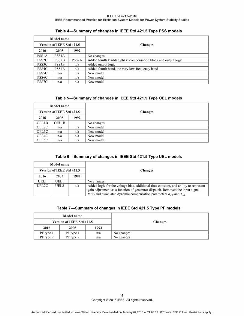
Table 4 —Summary of changes in IEEE Std 421.5 Type PSS models
Model name Changes Version of IEEE Std 421.5
2016 2005 1992 PSS1A PSS1A No changes PSS2C PSS2B PSS2A Added fourth lead-lag phase compensation block and output logic PSS3C PSS3B n/a Added output logic PSS4C PSS4B n/a Added fourth band, the very low-frequency band PSS5C n/a n/a New model PSS6C n/a n/a New model PSS7C n/a n/a New model
Table 5 —Summary of changes in IEEE Std 421.5 Type OEL models
Model name Changes Version of IEEE Std 421.5
2016 2005 1992 OEL1B OEL1B No changes OEL2C n/a n/a New model OEL3C n/a n/a New model OEL4C n/a n/a New model OEL5C n/a n/a New model
Table 6 —Summary of changes in IEEE Std 421.5 Type UEL models
Model name Changes Version of IEEE Std 421.5
2016 2005 1992 UEL1 UEL1 No changes
UEL2C UEL2 n/a Added logic for the voltage bias, additional time constant, and ability to represent gain adjustment as a function of generator dispatch. Removed the input signal VFB and associated dynamic compensation parameters KFB and TUL.
Table 7 —Summary of changes in IEEE Std 421.5 Type PF models
Model name Changes Version of IEEE Std 421.5
2016 2005 1992 PF type 1 PF type 1 n/a No changes PF type 2 PF type 2 n/a No changes
Authorized licensed use limited to: Iowa State University. Downloaded on January 07,2018 at 21:03:12 UTC from IEEE Xplore. Restrictions apply.

IEEE Std 421.5-2016 IEEE Recommended Practice for Excitation System Models for Power System Stability Studies
6 Copyright © 2016 IEEE. All rights reserved.
Table 8 —Summary of changes in IEEE Std 421.5 Type VAR models
Model name Changes Version of IEEE Std 421.5
2016 2005 1992 VAR type 1 VAR type 1 n/a No changes VAR type 3 VAR type 2 n/a No changes
Table 9 —Summary of changes in IEEE Std 421.5 Type SCL models
Model name Changes Version of IEEE Std 421.5
2016 2005 1992 SCL1C n/a n/a New model SCL2C n/a n/a New model
2. Normative references
The following referenced documents are indispensable for the application of this document (i.e., they must be understood and used, so each referenced document is cited in text and its relationship to this document is explained). For dated references, only the edition cited applies. For undated references, the latest edition of the referenced document (including any amendments or corrigenda) applies.
IEEE Std 115™, IEEE Guide for Test Procedures for Synchronous Machines: Part I—Acceptance and Performance Testing and Part II—Test Procedures and Parameter Determination for Dynamic Analysis.2, 3
IEEE Std 421.1™, IEEE Standard Definitions for Excitation Systems for Synchronous Machines.
IEEE Std 421.2™, IEEE Guide for Identification, Testing, and Evaluation of the Dynamic Performance of Excitation Control Systems.
IEEE Std 421.4™, IEEE Guide for the Preparation of Excitation System Specifications.
3. Definitions, acronyms, and abbreviations
For the purposes of this document, the excitation system definitions presented in IEEE Std 421.1 apply. The IEEE Standards Dictionary Online should be consulted for terms not defined in IEEE Std 421.1.4
2 IEEE publications are available from The Institute of Electrica and Electronics Engineers (http://standards.ieee.org/). 3 The IEEE standards or products referred to in this clause are trademarks of The Institute of Electrical and Electronics Engineers, Inc. 4IEEE Standards Dictionary Online is available at: http://ieeexplore.ieee.org/xpls/dictionary.jsp.
Authorized licensed use limited to: Iowa State University. Downloaded on January 07,2018 at 21:03:12 UTC from IEEE Xplore. Restrictions apply.

IEEE Std 421.5-2016 IEEE Recommended Practice for Excitation System Models for Power System Stability Studies
4. Representation of synchronous machine excitation systems in power system studies
The general functional block diagram shown in Figure 1 indicates various synchronous machine excitation subsystems. These subsystems may include a terminal voltage transducer and load compensator, excitation control elements, an exciter, and, in many instances, a power system stabilizer. Supplementary discontinuous excitation control may also be employed. Models for all of these functions are presented in this recommended practice.
The synchronous machine terminal conditions, used as inputs to the different subsystems shown in Figure 1 (e.g., V, I, P, Q, pf, VSI) are usually measured or calculated from the generator potential and current transformer signals in the excitation system. In this standard, these values are considered to be the positive sequence, fundamental frequency components (phasor measurements) associated with these quantities.
Excitation control elements include both excitation regulating and stabilizing functions. The terms excitation system stabilizer and transient gain reduction are used to describe circuits in several of the models encompassed by “excitation control elements” in Figure 1 that affect the stability and response of those systems. Annex A describes nomenclature used in Figure 1.
Recently, modeling of field current limiters has become increasingly important, resulting in the expansion of Clause 10 and Clause 11 describing overexcitation and underexcitation limiters (OELs and UELs) respectively, and the addition of Clause 12 describing stator current limiters (SCLs). The individual excitation system models in this recommended practice show how the output signals from such limiters (VOEL, VUEL, and VSCL) would normally be connected.
The output of the OEL and UEL models may be received as an input to the excitation system (VOEL and VUEL) at various locations, either as a summing input or as a gated input; but, for any one application of the excitation system model, only one connection for the VOEL signal and one connection for the VUEL connection would be used. The selection of the connection location for each of these signals should be independent of each other.
Similar to the OEL and UEL models, the SCL model may represent either a summation point or a take-over action. But, unlike the OEL and UEL models, the SCL model should define the signal VSCLsum when representing a summation point action, but should define two signals, VSCLoel and VSCLuel, when representing a take-over action.
In the implementation of all of the models, provision should be made for handling zero values of parameters. For some zero values, it may be appropriate to bypass entire blocks of a model.
The per-unit system used for modeling the excitation system is described in Annex B.
7 Copyright © 2016 IEEE. All rights reserved.
Authorized licensed use limited to: Iowa State University. Downloaded on January 07,2018 at 21:03:12 UTC from IEEE Xplore. Restrictions apply.

IEEE Std 421.5-2016 IEEE Recommended Practice for Excitation System Models for Power System Stability Studies
EXCITATION CONTROL ELEMENTS
EXCITERSYNCHRONOUS MACHINE AND
POWER SYSTEMEFE IFD
EFD
VSI
CURRENT COMPENSATOR
VUEL
VC1
VST POWER SYSTEM STABILIZER
DISCONTINUOUS EXCITATION CONTROL
VOLTAGE MEASUREMENT TRANSDUCER
VC
VREF
VFE
VS
OVEREXCITATION LIMITER
UNDEREXCITATIONLIMITER
PF/VAr CONTROLLER
VOEL
Vpf/VAr
P, Q, V, I
Q, pf
V, I
STATOR CURRENTLIMITER
(VSCLsum) or(VSCLoel and VSCLuel)
P, Q, V, I
Figure 1 —Functional block diagram for synchronous machine excitation control system
Three distinctive types of excitation systems are identified on the basis of excitation power source:
Type DC excitation systems, which utilize a direct current generator with a commutator as the source of excitation system power (Clause 6)
Type AC excitation systems, which use an alternator and either stationary or rotating rectifiers to produce the direct current needed for the synchronous machine field (Clause 7)
Type ST excitation systems, in which excitation power is supplied through transformers or auxiliary generator windings and rectifiers (Clause 8)
8 Copyright © 2016 IEEE. All rights reserved.
Authorized licensed use limited to: Iowa State University. Downloaded on January 07,2018 at 21:03:12 UTC from IEEE Xplore. Restrictions apply.

IEEE Std 421.5-2016 IEEE Recommended Practice for Excitation System Models for Power System Stability Studies
The following key accessory functions common to most excitation systems are also identified and described:
Voltage sensing and load compensation (Clause 5)
Power system stabilizer (Clause 9)
Overexcitation limiter (Clause 10)
Underexcitation limiter (Clause 11)
Stator current limiter (Clause 12)
Power factor and var control (Clause 13)
Discontinuous excitation controls (Clause 14)
Modern excitation systems typically offer several different limiting functions such as OELs, UELs, stator current limiters (SCL), and volts-per-hertz (V/Hz) limiters. Previous versions of this recommended practice included models for the OEL and UEL, and this version is introducing models for the SCL, but not for the V/Hz limiter. This is not a reflection on the availability of V/Hz limiters in actual field installations, but rather on the industry’s ability to develop a consensus on standard models and block diagrams to represent them.
Therefore, it is expected that future revisions of this recommended practice might include additional models for the SCL and possibly introduce models for the V/Hz limiter. Generally speaking, limiters are connected to the excitation system models in one of three possible ways:
As an additional signal added to the voltage error calculation (AVR summing input)
As a take-over signal, input to a high- or low-value logic gate in the excitation system model
As part of an upper or lower limit in the excitation system model
Thus, it is expected that future revisions of this recommended practice might also require changes to the existing excitation system models to clearly indicate how these SCL and V/Hz limiter models would be connected.
Most excitation systems represented by the Type AC and ST models allow only positive current flow to the field winding of the machine, although some systems allow negative voltage forcing until the current decays to zero. Special provisions are made to allow the flow of negative field current when it is induced by the synchronous machine. Methods of accommodating this in the machine/excitation system interface for special studies are described in Annex G.
5. Synchronous machine terminal voltage transducer and current compensation models
5.1 Terminal voltage sensing time constant
The terminal voltage of the synchronous machine is sensed and is usually reduced to a dc quantity. While the filtering associated with the voltage transducer may be complex, it can usually be represented, for modeling purposes, by a single equivalent time constant TR shown in Figure 2. For many systems, this time constant is very small and provision should be made to set it to zero.
9 Copyright © 2016 IEEE. All rights reserved.
Authorized licensed use limited to: Iowa State University. Downloaded on January 07,2018 at 21:03:12 UTC from IEEE Xplore. Restrictions apply.

IEEE Std 421.5-2016 IEEE Recommended Practice for Excitation System Models for Power System Stability Studies
It is realized that, for some systems, there may be separate and different time constants associated with the functions of voltage sensing and current compensation (see 5.2). This distinction does not normally need to be considered for modeling and in this document only one equivalent time constant, TR, is used for the combined voltage sensing and compensation signal. Single-phase voltage and current sensing, in general, requires a longer time constant in the sensing circuitry to eliminate ripple.
5.2 Current compensation
Several types of compensation are available on most excitation systems. Synchronous machine active and reactive current compensation are the most common in modern digital controllers. Either droop compensation and/or line drop compensation may be used, simulating an impedance drop and effectively regulating a calculated voltage at some point other than the terminals of the machine.
Droop compensation takes its name from the drooping (declining) voltage profile with increasing power output on the unit. Line-drop compensation, also referred to as transformer-drop compensation, refers to the act of regulating voltage at a point partway within a generator’s step-up transformer or, less frequently, somewhere along the transmission system. This form of compensation produces a rising voltage profile at the generator terminals for increases in output power.
A block diagram of the terminal voltage transducer and the load compensator is shown in Figure 2. These model elements are common to all excitation system models described in this document. Note that TR is used to denote the equivalent time constant for the combined voltage sensing and compensation signal, as described in 5.1. The terminal voltage of the synchronous machine is sensed and is usually reduced to a dc quantity. While the filtering associated with the voltage transducer may be complex, it can usually be approximated, for modeling purposes, to the single time constant, TR, shown. For many systems, this time constant is very small and provision should be made to set it to zero.
Figure 2 represents legacy systems described by Rubenstein and Wakley [B48] and it should be noted that the actual implementation of current compensation in modern digital exciters might not follow this exact phasor calculation. When current compensation is not employed (RC = XC = 0), the block diagram reduces to a simple sensing circuit. When compensation is desired, the appropriate values of RC and XC are entered. In most cases, the value of RC is negligible, and usually neglected. In these cases, the reactive component of current is resolved to a scalar value, as is the terminal voltage. Care should be taken in order to have a consistent per-unit system utilized for the compensator parameters and the synchronous machine current base.
1
1+sTR
VCVC1
VT–
–IT
–VC1=|VT+(RC+jXC)∙IT|
–
Figure 2 —Terminal voltage transducer and optional current-compensation
elements
The terminal voltage transducer output, VC, is compared with a reference that represents the desired terminal voltage setting, as shown on each of the excitation system models. The equivalent voltage regulator reference signal, VREF, is calculated to satisfy the initial operating conditions. Therefore, it takes on a value unique to the synchronous machine load condition being studied. The resulting error is amplified as described in the appropriate excitation system model to provide the field voltage and subsequent terminal voltage to satisfy the steady-state loop equations. Without current compensation, the excitation system, within its regulation characteristics, attempts to maintain a terminal voltage determined by the reference signal.
10 Copyright © 2016 IEEE. All rights reserved.
Authorized licensed use limited to: Iowa State University. Downloaded on January 07,2018 at 21:03:12 UTC from IEEE Xplore. Restrictions apply.

IEEE Std 421.5-2016 IEEE Recommended Practice for Excitation System Models for Power System Stability Studies
This type of compensation is normally used in one of the following two ways:
a) Droop compensation—When synchronous machines are connected to the same terminal bus with no impedance between them, droop compensation is used to create artificial coupling impedance so that the machines will share reactive power appropriately and is mandatory for the stable operation of these parallel units. This corresponds to the choice of a regulating point within the synchronous machine. For this case, XC would be a positive value and RC would be greater than or equal to zero.
b) Line drop compensation—When a single synchronous machine is connected through significant impedance to the system, or when two or more machines are connected through individual transformers, it may be desirable to regulate voltage at a point beyond the machine terminals. For example, it may be desirable to compensate for a portion of the transformer impedance and effectively regulate voltage at a point part way through the step-up transformer. For these cases, XC would be an appropriate negative value, while RC would be less than or equal to zero.
Some compensator circuits act to modify terminal voltage as a function of reactive and real power, instead of reactive and real components of current. Although the model provided in Figure 2 is equivalent to these circuits only near rated terminal voltage, more precise representation has not been deemed worthwhile. These and other forms of compensation are described by Rubenstein and Wakley [B48].
5.2.1 Cross-current compensation
The AVR feedback signal can include inputs from other synchronous machines when the machines are connected together on a low-voltage bus and share a common main output transformer. A general form of the AVR feedback signal for unit 1, VC1, is shown in Equation (1).
( ) ( ) 21212111111 TCCTCCTC IjXRIjXRVV ++++= (1)
where
TV is the ac terminal voltage (phasor) common to both generators
TiI is the ac terminal current (phasor) flowing out of generator i
CijR is the resistive component of compensation of generator i for current flow out of generator j
CijX is the reactive component of compensation of generator i for current flow out of generator j
The subscripts identify the signals associated with each of the two generators. The first subscript indicates the unit to which the load compensation is connected, while the second subscript indicates the source of the current signal to the compensation. This is the general form of the single machine compensation (i.e., with RC12, XC12 equal to zero). A similar equation applies to the AVR input for the second unit with appropriate substitution of inputs and subscripts. This can be readily extended to more generators by including additional compensation terms.
In practice, the resistive component of compensation is rarely required on generators synchronized to large grids over high-voltage interconnections. This component of compensation is not even available on some manufacturers’ designs. To simplify analysis, the resistive component of compensation is assumed to be zero, and the current signals are resolved into two components, shown in Equation (2).
11 Copyright © 2016 IEEE. All rights reserved.
Authorized licensed use limited to: Iowa State University. Downloaded on January 07,2018 at 21:03:12 UTC from IEEE Xplore. Restrictions apply.

IEEE Std 421.5-2016 IEEE Recommended Practice for Excitation System Models for Power System Stability Studies
12 Copyright © 2016 IEEE. All rights reserved.
T
T
T
TQP
T
TT
T
TT
V
Qj
V
PjII
V
jQP
V
SI −=−=−==
*
(2)
where
TV is the magnitude of the ac terminal voltage (phasor) of the generator
TI is the ac terminal current (phasor) flowing out of the generator, considering the terminal voltage
of the generator as the reference for phasor angles *TS is the complex conjugate of the ac apparent power output flowing out of the generator
TP is the active power output flowing out of the generator
TQ is the reactive power output flowing out of the generator
PI is the active current component of the terminal current, the component in phase with the terminal
voltage, and thus corresponding to the active power flowing out of the generator
QI is the reactive current component of the terminal current, the component in quadrature with the
terminal voltage, and thus corresponding to the reactive power flowing out of the generator
When the current flowing out of the generator lags the voltage, the synchronous machine is operating in an overexcited mode and the reactive power output of the machine is considered positive, as shown in Equation (2). It is a common practice to consider the reactive component of the current (IQ) and the associated reactive power (QT) both as positive values when terminal current lags the voltage, simply adjusting the phasor calculations as necessary. For relatively constant terminal voltage (i.e., changes of no more than a few percent from the nominal level), the amplitude of the active and reactive components of current is equal to the active and reactive power output of the generator when expressed in per-unit.
Disregarding the resistive components of the compensation and using the definition of the active and reactive components of the current from Equation (2), Equation (1) can be simplified as shown in Equation (3):
( ) ( ) 2121112121112121111 QCQCTPCPCQCQCTC IXIXVIXIXjIXIXVV ++≈++++= (3)
where all variables have been previously defined in Equation (1) and Equation (2).
The latter approximation is based on the fact that changes in the active component of current have relatively little effect on the compensated voltage amplitude. On most modern digital systems, this algebraic equation is an exact representation of the compensated voltage (VC1) used as the AVR input signal, as the reactive component is resolved and multiplied by the compensation and then combined with the terminal voltage signal.
Referring to Equation (3), when the selected compensation is positive and the reactive current lags the voltage, the compensated voltage (VC1) becomes greater than the magnitude of the terminal voltage (VT). When a larger value VC1 is presented to the AVR feedback input, the result is a reduction in excitation. Based on this, the type of compensation can be categorized as follows:
a) XC11 > 0, XC12 = 0 Commonly referred to as reactive droop. The generator terminal voltage will exhibit a declining or drooping characteristic as reactive output increases.
b) XC11 < 0, XC12 = 0 Commonly referred to as transformer-drop or line-drop compensation. The generator terminal voltage will exhibit a rising characteristic as reactive output increases.
Authorized licensed use limited to: Iowa State University. Downloaded on January 07,2018 at 21:03:12 UTC from IEEE Xplore. Restrictions apply.

IEEE Std 421.5-2016 IEEE Recommended Practice for Excitation System Models for Power System Stability Studies
c) XC11 ≠ 0, XC12 ≠ 0 Commonly referred as cross-current compensation, although the preferred terminology is reactive differential compensation. Through careful selection of the two coefficients (e.g., XC12 = –XC11) this form of compensation can be used to offset or eliminate the drooping voltage characteristic while enforcing reactive current sharing between synchronous machines sharing a common low-voltage connection.
6. Type DC—Direct current commutator rotating exciter
6.1 General
Few new synchronous machines are being equipped with Type DC exciters, which have been superseded by type AC and ST systems, however many such systems are still in service. Considering the dwindling percentage and importance of units equipped with these exciters, the previously developed concept (see IEEE Committee Report, 1968 [B21]) of accounting for loading effects on the exciter by using the loaded saturation curve (Annex C) is considered adequate. Figure 3 presents the model used to represent a dc rotating exciter, which is used in all Type DC excitation system models, which may be either separately excited or self-excited as discussed in the 1981 IEEE Committee Report [B23]. When a self-excited shunt field is used, the value of the feedback gain KE reflects the setting of the shunt field rheostat. In some instances, the resulting value of KE can be negative and allowance should be made for this.
Most of these exciters utilize self-excited shunt fields with the voltage regulator operating in a mode commonly termed buck-boost. The majority of station operators manually track the voltage regulator by periodically trimming the rheostat set point so as to zero the voltage regulator output. This may be simulated by selecting the value of KE so that initial conditions are satisfied with EFE = 0, as described in the 1981 IEEE Committee Report [B23]. In some programs, if KE is entered as zero, KE is automatically calculated by the program to represent a self-excited shunt field and a trimmed rheostat as its initial condition.
If a non-zero value for KE is provided, the program should not recalculate KE, as a fixed rheostat setting is implied. For such systems, the rheostat is frequently fixed at a value that would produce self-excitation near rated conditions. Systems with fixed field rheostat settings are in widespread use on units that are remotely controlled.
A separately-excited dc rotating exciter is represented by a value for KE = 1.
The term SE(EFD) is a non-linear function with values defined at two or more chosen values of generator field voltage EFD, as described in Annex C. The output of this saturation block VX is the product of the input EFD and the value of the non-linear function SE(EFD) at this exciter output voltage.
13 Copyright © 2016 IEEE. All rights reserved.
Authorized licensed use limited to: Iowa State University. Downloaded on January 07,2018 at 21:03:12 UTC from IEEE Xplore. Restrictions apply.

IEEE Std 421.5-2016 IEEE Recommended Practice for Excitation System Models for Power System Stability Studies
++
VFE
EFDEFE
VX(a)
Σ
Σ
1
sTE
EFDmin
KE
–+
SE(EFD)
footnotes:
VX = EFD∙ΣE(EFD)(a) Figure 3 —DC commutator rotating exciter model
The representation of an excitation system with a dc commutator rotating exciter is not confined to using a Type DC model. Digitally based voltage regulators feeding dc rotating main exciters can also be represented with a Type AC excitation system model (e.g., AC6C or AC8C) by simply setting the parameters KC and KD in the type ac rotating exciter model to zero (see Figure 8). Also, if a more detailed representation of a dc rotating main exciter is desired, a suitable Type AC model with values for KD and/or KC can be applied.
The relationships between regulator limits and field voltage limits are developed in the 1981 IEEE Committee Report [B23].
Excitation systems incorporating rotating machines produce a field voltage output (EFD) which is proportional to the rotating speed of the machine. This effect is negligible where speed deviations are small as is typical for dynamic studies of large, interconnected power systems. However, introduction of a per-unit speed multiplier for field voltage might improve the simulation accuracy of off-nominal frequency events, such as system islanding, or open-circuit operation, where the unit speed may vary significantly.
This revision of the recommended practice does not represent the effect of speed deviations on the output of the dc rotating exciter models, but it should be noted that provision for the speed dependency may be found in some model implementations in commercial software.
Sample data for the models presented in this clause are presented in Annex H.
6.2 Type DC1A excitation system model
The DC1A excitation system model defined in the previous version of this recommended practice is being superseded by the model DC1C shown in 6.3. Any existing excitation system represented by the DC1A model could also be represented by the DC1C model with the same parameters, just defining the new parameter EFDmin = –99 pu (large negative value). The major differences between the DC1A and DC1C models are related to additional options for the connection of OEL models, introduced in the new DC1C model. Refer to Table 1 for a summary of the changes in the models.
6.3 Type DC1C excitation system model
This model, described by the block diagram of Figure 4, is used to represent field controlled dc commutator exciters with continuously acting voltage regulators (especially the direct-acting rheostatic, rotating amplifier, and magnetic amplifier types).
14 Copyright © 2016 IEEE. All rights reserved.
Authorized licensed use limited to: Iowa State University. Downloaded on January 07,2018 at 21:03:12 UTC from IEEE Xplore. Restrictions apply.

IEEE Std 421.5-2016 IEEE Recommended Practice for Excitation System Models for Power System Stability Studies
The principal input to this model is the output from the terminal voltage transducer and current compensator model VC described in Clause 5. At the summing junction, the terminal voltage transducer output VC is subtracted from the voltage reference set point VREF. The stabilizing feedback signal VF is subtracted and the power system stabilizer output signal VS, if present, is added to produce an error voltage. Similarly, limiters represented as summation point actions (VOEL, VUEL, and/or VSCLsum) are also added to the calculation of the voltage error. In steady state, these last signals (VF and VS, VOEL, VUEL, and VSCLsum) are zero, leaving only the terminal voltage error signal. The resulting signal is amplified in the regulator. The major time constant TA and gain KA associated with the voltage regulator are shown incorporating non-windup limits typical of saturation or amplifier power supply limitations. A discussion of windup and non-windup limits is provided in Annex E. These voltage regulators utilize power sources that are essentially unaffected by brief transients on the synchronous machine or auxiliaries buses. The time constants, TB and TC, may be used to model equivalent time constants inherent in the voltage regulator; but these time constants are frequently small enough to be neglected and provision should be made for zero input data.
KA
1+sTA
VRmax
VRmin
1+sTC
1+sTB
VUEL VOEL
bb
sKF
1+sTF
++
VFE
EFDEFE
VX(a)
Σ
Σ
1
sTE
EFDmin
KE
–+
footnotes:
SE(EFD)
VX = EFD∙ΣE(EFD)(a)
summation pointa
b take-over
alternateOEL input locations
(VOEL)
summation pointa
b take-over
alternateUEL input locations
(VUEL)
summation pointa
b take-over
alternateSCL input locations
(VSCL)
VOELsclVUELscl
b b
HV gate
LV gate
VF
ΣVC
VREF
VS
–
VUEL
+
+
+ +
+–
aa
Σ+
VSCLsum
aa
VOEL
Figure 4 —Type DC1C dc commutator exciter
The voltage regulator output (or exciter field voltage, EFE), is used to control the dc rotating exciter.
A signal derived from generator field voltage is normally used to provide excitation system stabilization (VF) via the rate feedback block with gain KF and time constant TF.
The block diagram shown in Figure 4 has been modified, as compared to the DC1A block diagram defined in the previous version of this recommended practice, to include the appropriate connections for summation point or take-over overexcitation limiters and the lower limit EFDmin.
15 Copyright © 2016 IEEE. All rights reserved.
Authorized licensed use limited to: Iowa State University. Downloaded on January 07,2018 at 21:03:12 UTC from IEEE Xplore. Restrictions apply.

IEEE Std 421.5-2016 IEEE Recommended Practice for Excitation System Models for Power System Stability Studies
6.4 Type DC2A excitation system model
The DC2A excitation system model defined in the previous version of this recommended practice is being superseded by the model DC2C shown in 6.5. Any existing excitation system represented by the DC2A model could also be represented by the DC2C model with the same parameters, defining the new parameter EFDmin = –99 pu (large negative value). The major differences between the DC2A and DC2C models are related to additional options for the connection of OEL models, introduced in the new DC2C model. Refer to Table 1 for a summary of the changes in the models.
6.5 Type DC2C excitation system model
The model shown in Figure 5 is used to represent field-controlled dc commutator exciters with continuously acting voltage regulators having power supplies derived from the generator or auxiliaries bus. It differs from the Type DC1A model only in the voltage regulator output limits, which are now proportional to terminal voltage magnitude VT.
It is representative of solid-state replacements for various forms of older mechanical and rotating amplifier regulating equipment connected to dc commutator exciters.
The block diagram shown in Figure 5 has been modified, as compared to the DC2A block diagram defined in previous version of this recommended practice, to include the appropriate connections for summation point or take-over overexcitation limiters, and the addition of a lower limit EFDmin.
KA
1+sTA
VT.VRmax
1+sTC
1+sTB
VUEL VOEL
bb
sKF
1+sTF
++
VFE
EFDEFE
VX(a)
Σ
Σ
1
sTE
EFDmin
KE
–+
footnotes:
SE(EFD)
VX = EFD∙ΣE(EFD)(a)
summation pointa
b take-over
alternateOEL input locations
(VOEL)
summation pointa
b take-over
alternateUEL input locations
(VUEL)
summation pointa
b take-over
alternateSCL input locations
(VSCL)
VOELsclVUELscl
b b
HV gate
LV gate
VF
ΣVC
VREF
VS
–
VUEL
+
+
+ +
+–
aa
Σ+
VSCLsum
aa
VOEL
VT.VRmin
Figure 5 —Type DC2C dc commutator exciter with bus-fed regulator
16 Copyright © 2016 IEEE. All rights reserved.
Authorized licensed use limited to: Iowa State University. Downloaded on January 07,2018 at 21:03:12 UTC from IEEE Xplore. Restrictions apply.

IEEE Std 421.5-2016 IEEE Recommended Practice for Excitation System Models for Power System Stability Studies
6.6 Type DC3A excitation system model
The systems discussed in the previous clauses are representative of the first generation of high gain, fast-acting excitation sources. The Type DC3A model is used to represent older systems, in particular those dc commutator exciters with non-continuously acting regulators that were commonly used before the development of the continuously acting varieties.
These systems respond at basically two different rates, depending upon the magnitude of voltage error. For small errors, adjustment is made periodically with a signal to a motor-operated rheostat. Larger errors cause resistors to be quickly shorted or inserted and a strong forcing signal applied to the exciter. Continuous motion of the motor-operated rheostat occurs for these larger error signals, even though it is bypassed by contactor action. Figure 6 illustrates this control action.
The dc rotating exciter representation is described in 6.1 and its block diagram is shown in Figure 3. Note that no excitation system stabilizer is represented.
Depending upon the magnitude of voltage error, VREF – VC, different regulator modes come into play. If the voltage error is larger than the fast raise/lower contact setting, KV (typically 5%), VRmax, or VRmin is applied to the exciter, depending upon the sign of the voltage error. For an absolute value of voltage error less than KV, the exciter input equals the rheostat setting VRH. The rheostat setting is notched up or down, depending upon the sign of the error. The travel time representing continuous motion of the rheostat drive motor is TRH. A non-windup limit (see Annex E) is shown around this block, to represent the fact that when the rheostat reaches either limit, it is ready to come off the limit immediately when the input signal reverses.
The model assumes that the quick raise-lower limits are the same as the rheostat limits. In actual electro-mechanical and analog-electronic implementations, there is a smaller deadband KR on the error signal VERR so there is no change of exciter field voltage while the voltage error is within this deadband. This deadband is represented in the older IEEE Type 4 model (IEEE Committee Report, 1968 [B2]) which may be used to represent some older equipment still in service. More modern systems utilize feedback or feed-forward stabilization, rather than relying on this deadband for stability.
The model does not account for changes in the exciter field time constant as a result of changes in field resistance (as a result of rheostat movement and operation of quick action contacts).
+–
VC
VREF
VRmax−VRmin
sKVTRH
IF VERR > KV, VR=VRmaxIF |VERR| < KV, VR=VRHIF VERR < −KV, VR=VRmin
KV
−KV
VERR VRH
VRmax
VRmin
Σ
VR
++
VFE
EFD
VX(a)
Σ
Σ
1
sTE
KE
–+
footnotes:SE(EFD)
VX = EFD∙ΣE(EFD)(a) Figure 6 —Type DC3A dc commutator exciter with non-continuously acting regulators
17 Copyright © 2016 IEEE. All rights reserved.
Authorized licensed use limited to: Iowa State University. Downloaded on January 07,2018 at 21:03:12 UTC from IEEE Xplore. Restrictions apply.

IEEE Std 421.5-2016 IEEE Recommended Practice for Excitation System Models for Power System Stability Studies
6.7 Type DC4B excitation system model
The DC4B excitation system model defined in the previous version of this recommended practice is being superseded by the model DC4C shown in 6.8. Any existing excitation system represented by the DC4B model could also be represented by the DC4C model, with practically the same parameters. The differences between the DC4B and DC4C models are mostly related to additional options for the connection of summation point UEL and OEL models, introduced in the new DC4C model.
Furthermore, the DC4C model offers a more flexible representation of the power source for the controlled rectifier connected to the rotating exciter field winding. Refer to Table 1 for a summary of the changes in the models.
Because of the new representation of the power source of the controlled rectifier, the DC4C model requires additional parameters, as compared to the DC4B model. Thus, the conversion of existing DC4B data into the new DC4C model would require setting KP = 1, θP = 0, KI = XL = KC1 = 0, VBmax = 99 pu (large number), and selecting the logic SW1 in position “A.”
6.8 Type DC4C excitation system model
These excitation systems utilize a field-controlled dc commutator exciter with a continuously acting voltage regulator having supplies obtained from the generator or auxiliary services bus. The replacement of the controls only as an upgrade (retaining the dc commutator exciter) has resulted in a new model. The block diagram of this model is shown in Figure 7. This excitation system typically includes a PID automatic voltage regulator (AVR). An alternative rate feedback loop (KF, TF) for stabilization is also shown in the model if the AVR does not include a derivative term.
The block diagram shown in Figure 7 has been modified, as compared to the previous version of this recommended practice, by changing the sign of the connection of the summation point overexcitation limiter VOEL.
18 Copyright © 2016 IEEE. All rights reserved.
Authorized licensed use limited to: Iowa State University. Downloaded on January 07,2018 at 21:03:12 UTC from IEEE Xplore. Restrictions apply.

IEEE Std 421.5-2016 IEEE Recommended Practice for Excitation System Models for Power System Stability Studies
VRmax/KA
VRmin/KA
Π
FEX1=f(IN1)
FEX1
IN1
VE
VBmax
KP
VB
y
ΠSW1
(a)
VFE
KA
1+sTA
VRmax
VRmin
VR
++
VFE
EFDEFE
VX(b)
Σ
Σ
1
sTE
EFDmin
KE
–+
sKF
1+sTF
KP=KP θP–
y=|KP∙VT+j(KI+KP∙XL)∙IT|– – ––
IN1=KC1VFE
VE
SE(EFD)
–IT
VT– A
B
VUEL VOEL
bb
VOELsclVUELscl
b b
HV gate
LV gateKPR+
KIR+
s
sKDR
1+sTDR
VF
ΣVC
VREF
VS
–
VUEL
+
+
+ +
+–
aa
Σ+
VSCLsum
aa
VOEL
footnotes:
VX = EFD∙ΣE(EFD)(b)
summation pointa
b take-over
alternateOEL input locations
(VOEL)
summation pointa
b take-over
alternateUEL input locations
(VUEL)
summation pointa
b take-over
alternateSCL input locations
(VSCL)
SW1 is a user-selection option. Position A corresponds to a power source derived from generator terminal voltage, such as an excitation transformer. Position B corresponds to a power source independent of generator terminal conditions, such as a pilot exciter.
(a)
Figure 7 —Type DC4C dc commutator exciter with PID style regulator
This excitation system model is an extension of the DC4B model to include the representation of the power source for the controlled rectifier, as well as the rectifier loading and commutation effects are accounted for as described in Annex D. The logic switch SW1 determines if the power source of the controlled rectifier is derived from terminal voltage (position A) or is independent of the terminal voltage (position B). The function FEX1 is the same function FEX shown in Annex D, but the input to the function IN1 should be calculated based on the exciter field current VFE instead of the generator field current IFD.
The DC4C model could be used to represent any equipment currently represented by the DC4B model. The DC4B model considers a simplified representation of the power source as derived from the generator terminal voltage. Thus, the logic SW1 in the DC4C model should be set to position “A,” and KP = 1, θP = 0, KI = XL = KC1 = 0, VBmax = 99 pu (large number).
19 Copyright © 2016 IEEE. All rights reserved.
Authorized licensed use limited to: Iowa State University. Downloaded on January 07,2018 at 21:03:12 UTC from IEEE Xplore. Restrictions apply.

IEEE Std 421.5-2016 IEEE Recommended Practice for Excitation System Models for Power System Stability Studies
7. Type AC—Alternator supplied rectifier excitation systems
7.1 General
These excitation systems use an ac alternator and either stationary or rotating rectifiers to produce the dc generator field requirements. Loading effects on such exciters are significant, and the use of generator field current as an input to the models allows these effects to be represented accurately. These systems do not allow the supply of negative field current, and only the Type AC4C model allows negative generator field voltage forcing. Modeling considerations for induced negative field currents are discussed in Annex G. If these models are being used to design phase lead networks for power system stabilizers, and the local mode is close to 3 Hz or higher, a more detailed treatment of the ac rotating exciter may be needed. However, the models should be satisfactory for large-scale simulations.
Figure 8 presents the block diagram of the model for the ac rotating exciter with non-controlled rectifiers (see Ferguson, Herbst, and Miller [B13] and Gayek [B14]). The demagnetizing effect of load current IFD on the exciter alternator output voltage VE is accounted for in the feedback path that includes the demagnetization constant KD. This constant depends on of the exciter alternator synchronous and transient reactances (see Ferguson, Herbst, and Miller [B13] and Gayek [B14]). A signal proportional to exciter field current VFE is derived from the summation of signals from exciter output voltage VE multiplied by KE + SE(VE) and generator field current IFD multiplied by the demagnetization term KD.
The term SE(VE) represents saturation as described in Annex C. In some of the models, the exciter field current signal VFE is used as the input to the excitation system stabilizing block with output VF.
The diode characteristic in the exciter output imposes a lower limit of zero on the exciter output voltage, so the lower limit VEmin should typically be set equal to zero. Exciter output voltage drop due to rectifier regulation is simulated by inclusion of the constant KC (which is a function of commutating reactance) and the rectifier regulation curve FEX as described in Annex D.
The upper limit VFEmax represents a limit in the exciter field current VFE. This limit can represent an instantaneous exciter field current limit, particularly if no explicit model for the overexcitation limiter, such as those models presented in Clause 10, is being represented. If an explicit OEL model is applied, and the OEL model represents the instantaneous field current limit, the user should set VFEmax = 99 pu (large number) to avoid conflicts between these limiter actions.
Excitation systems incorporating rotating machines produce a voltage output EFD which is proportional to the rotating speed of the machine. For dynamic studies of large, interconnected power systems, or where speed-deviations are very small, this effect is negligible. However, introduction of a per-unit speed multiplier for field voltage might improve the accurate simulation of off-nominal frequency events, such as system islanding or open-circuit operation, where the unit speed may vary significantly.
This revision of the recommended practice does not represent the effect of speed deviations on the output of the ac rotating exciter models, but it should be noted that provision for the speed dependency may be found in some model implementations in commercial software.
Sample data for the models presented in this clause are presented in Annex H.
20 Copyright © 2016 IEEE. All rights reserved.
Authorized licensed use limited to: Iowa State University. Downloaded on January 07,2018 at 21:03:12 UTC from IEEE Xplore. Restrictions apply.

IEEE Std 421.5-2016 IEEE Recommended Practice for Excitation System Models for Power System Stability Studies
FEX=f(IN)
FEX
IN
++
VFE
EFE
VX(a)
Σ
Σ
1
sTE
VEmin
KE
–+
SE(VE)
Π
KD
IN=KC∙IFD
VE
+
IFD
EFDVE
VFEmax−KD∙IFD
KE+SE(VE)
footnotes:
VX = VE∙ΣE(VE)(a) Figure 8 —AC rotating exciter with non-controlled rectifier model
7.2 Type AC1A excitation system model
The AC1A excitation system model defined in the previous version of this recommended practice is being superseded by the model AC1C shown in 7.3. Any existing excitation system represented by the AC1A model could also be represented by the AC1C model, with practically the same parameters.
The differences between the AC1A and AC1C models are mostly related to additional options for the connection of summation point UEL and OEL models, introduced in the new AC1C model, but it should be noted that the exciter field voltage limits VRmax and VRmin in the AC1A model have been renamed as EFEmax and EFEmin, respectively, in the AC1C model. Additional parameters VEmin and VFEmax have been introduced in the AC1C model, and these parameters should be set to VEmin = 0 and VFEmax = 99 pu (large number) in the AC1C model to match the block diagram of the AC1A model. Refer to Table 2 for a summary of the changes in the Type AC models.
7.3 Type AC1C excitation system model
The model shown in Figure 9 represents the field-controlled alternator rectifier excitation systems designated Type AC1C. These excitation systems consist of an alternator main exciter feeding its output via non-controlled rectifiers. The exciter does not employ self-excitation, and the voltage regulator power is taken from a source that is not affected by external transients.
For large power system stability studies, the exciter alternator and rectifier can be represented by the simplified model shown in Figure 8.
The block diagram shown in Figure 9 has been modified, as compared to the AC1A block diagram defined in the previous version of this recommended practice, to include the appropriate connections for summation point overexcitation limiters and underexcitation limiters. Additionally, the lower and upper limits of the rotating exciter are now defined by the parameters VEmin and VFEmax, respectively, as shown in Figure 8. Thus, converting data from the AC1A model into the AC1C model would require setting VEmin = 0 and VFEmax = 99 pu (large number).
21 Copyright © 2016 IEEE. All rights reserved.
Authorized licensed use limited to: Iowa State University. Downloaded on January 07,2018 at 21:03:12 UTC from IEEE Xplore. Restrictions apply.

IEEE Std 421.5-2016 IEEE Recommended Practice for Excitation System Models for Power System Stability Studies
VF
VA
EFEmax
EFEmin
VFE
EFE
IFD
EFD
sKF
1+sTF
HV gate
bb
1+sTC
1+sTB
KA
1+sTA
VAmax
VAmin
VUEL VOEL
ΣVC
VREF
VS
–
VUEL VOEL
+
+
+ ++
–
aa
Σ
footnotes:
summation pointa
b take-over
alternateOEL input locations
(VOEL)
alternateUEL input locations
(VUEL)
LV gate
AC rotating exciter
(a)
The AC rotating exciter block diagram is presented in Figure 8(a)
b
VSCLuel
b
VSCLoelVSCLsum
a
+
summation pointa
b take-over
alternateSCL input locations
(VSCL)
summation pointa
b take-over
Figure 9 —Type AC1C alternator-rectifier excitation system with non-controlled
rectifiers and feedback from exciter field current
7.4 Type AC2A excitation system model
The AC2A excitation system model defined in the previous version of this recommended practice is being superseded by the model AC2C shown in 7.5. Any existing excitation system represented by the AC2A model could also be represented by the AC2C model, with practically the same parameters. The major differences between the AC2A and AC2C models are related to additional options for the connection of summation point UEL and OEL models, introduced in the new AC2C model. A new parameter VEmin has been introduced to represent the lower limit on the output of the rotating exciter. The diode characteristic in the exciter output imposes a lower limit of zero on the exciter output voltage, so the lower limit VEmin should typically be set equal to zero, for brushless rotating exciters. Refer to Table 2 for a summary of the changes in the Type AC models.
7.5 Type AC2C excitation system model
The model shown in Figure 10, designated as Type AC2C, represents a high initial response field-controlled alternator-rectifier excitation system. The alternator main exciter is used, feeding its output via non-controlled rectifiers. The Type AC2C model is similar to that of Type AC1C except for the inclusion of exciter time constant compensation and exciter field current limiting elements.
The exciter time constant compensation consists essentially of a direct negative feedback VH around the exciter field time constant TE, reducing its effective value and thereby increasing the small signal response bandwidth of the excitation system. The time constant is reduced by a factor proportional to the product of gains KB and KH of the compensation loop and is normally more than an order of magnitude lower than the time constant without compensation.
To obtain high initial response with this system, a very high pu forcing voltage limit EFEmax is applied to the exciter field. A limiter-sensing exciter field current serves to allow high forcing but limit the current. By limiting the exciter field current, exciter output voltage VE is limited to a selected value, which is usually determined by the specified excitation system nominal response. Although this limit is realized physically
22 Copyright © 2016 IEEE. All rights reserved.
Authorized licensed use limited to: Iowa State University. Downloaded on January 07,2018 at 21:03:12 UTC from IEEE Xplore. Restrictions apply.

IEEE Std 421.5-2016 IEEE Recommended Practice for Excitation System Models for Power System Stability Studies
by a feedback loop as described in Annex F, the time constants associated with the loop can be extremely small and can cause computational problems. For this reason, the limiter is shown in the model as a positive limit on exciter voltage back of commutating reactance, which is in turn a function of generator field current. For small limiter loop time constants this has the same effect, but it circumvents the computational problem associated with the high gain, small time constant loop.
The limits on VE are used to represent the effects of feedback limiter operation, as described in Annex F.
The block diagram shown in Figure 10 has been modified, as compared to the AC2A block diagram defined in the previous version of this recommended practice, to include the appropriate connections for summation point overexcitation limiters and underexcitation limiters.
VF
VA
EFEmax
EFEmin
VFE
EFE
sKF
1+sTF
HV gate
bb
1+sTC
1+sTB
KA
1+sTA
VAmax
VAmin
VUEL VOEL
ΣVC
VREF
VS
–
VUEL VOEL
+
+
+ +
+–
aa
Σ
footnotes:
LV gate
KH
KBΣ
–+
VH
VOELsclVUELscl
b bIFD
EFDAC rotating exciter
(a)
The AC rotating exciter block diagram is presented in Figure 8(a)
+
VSCLsum
a
summation pointa
b take-over
alternateOEL input locations
(VOEL)
summation pointa
b take-over
alternateUEL input locations
(VUEL)
summation pointa
b take-over
alternateSCL input locations
(VSCL)
Figure 10 —Type AC2C high initial response alternator-rectifier excitation system with
non-controlled rectifiers and feedback from exciter field current
7.6 Type AC3A excitation system model
The AC3A excitation system model defined in the previous version of this recommended practice is being superseded by the model AC3C shown in 7.7. The only differences between the AC3A and AC3C models are related to additional options for the connection of summation point UEL and OEL models and takeover OEL model, introduced in the new AC3C model, and the addition of a PID controller to allow the representation of retrofit projects where a modern digital controller is added to the original exciter. Any existing excitation system represented by the AC3A model could also be represented by the AC3C model, with practically the same parameters. The additional parameters for the PID controller should be set as KPR = 1, KIR = 0, KDR = 0, TDR = 0.1, VPIDmax = 99 pu (large number) and VPIDmin = –99 pu (large negative number). Refer to Table 2 for a summary of the changes in the Type AC models.
23 Copyright © 2016 IEEE. All rights reserved.
Authorized licensed use limited to: Iowa State University. Downloaded on January 07,2018 at 21:03:12 UTC from IEEE Xplore. Restrictions apply.

IEEE Std 421.5-2016 IEEE Recommended Practice for Excitation System Models for Power System Stability Studies
7.7 Type AC3C excitation system model
The model shown in Figure 11 represents the field-controlled alternator-rectifier excitation systems designated Type AC3C. These excitation systems include an alternator main exciter feeding its output via non-controlled rectifiers. The exciter employs self-excitation and the voltage regulator power is derived from the exciter output voltage. Therefore, this system has an additional non-linearity, simulated by the use of a multiplier whose inputs are the voltage regulator command signal (VA) and the exciter output voltage (EFD) times KR. This model is applicable to excitation systems employing static voltage regulators.
For large power system stability studies, the simplified exciter alternator synchronous machine model shown in Figure 8 can be used.
The excitation system stabilizer in this model has a non-linear characteristic. The feedback gain is KF with exciter output voltage less than EFDN. When exciter output voltage exceeds EFDN, the value of the feedback gain becomes KN.
The block diagram shown in Figure 11 has been modified, as compared to the AC3A block diagram defined in the previous version of this recommended practice, to include the appropriate connections for summation point overexcitation limiters and underexcitation limiters, and takeover overexcitation limiters and the addition of the PID control structure that can be used to represent retrofit projects where a modern digital controller has been installed on the original rotating exciter.
Π
VF
HV gate
bb
1+sTC
1+sTB
VUEL VOEL
Σ
VREF
–
+
+
+–
LV gate VA
KA
1+sTA
VAmax
VAmin
Σ
s
1+sTF
KR
VPIDmax
VPIDmin
VN
EFDEFDN
KF
KN
+
+
a
VUEL
a
VOEL
VSCLsum
a
+
b
VSCLuel
b
VSCLoel
KIR
s
sKDR
1+sTDR+KPR +Σ
VC
VS
+
summation pointa
b take-over
alternateOEL input locations
(VOEL)
summation pointa
b take-over
alternateUEL input locations
(VUEL)
summation pointa
b take-over
alternateSCL input locations
(VSCL)
VFE
EFE
EFD
AC rotating exciter
(a)IFD
footnotes:(a) The AC rotating exciter block diagram is presented in Figure 8
VN
Figure 11 —Type AC3C alternator-rectifier exciter with alternator field current limiter
7.8 Type AC4A excitation system model
The AC4A excitation system model defined in the previous version of this recommended practice is being superseded by the model AC4C shown in 7.9. Any existing excitation system represented by the AC4A model could also be represented by the AC4C model, with exactly the same parameters. The only differences between the AC4A and AC4C models are related to additional options for the connection of summation point UEL and OEL models and takeover OEL model, introduced in the new AC4C model. Refer to Table 2 for a summary of the changes in the Type AC models.
24 Copyright © 2016 IEEE. All rights reserved.
Authorized licensed use limited to: Iowa State University. Downloaded on January 07,2018 at 21:03:12 UTC from IEEE Xplore. Restrictions apply.

IEEE Std 421.5-2016 IEEE Recommended Practice for Excitation System Models for Power System Stability Studies
7.9 Type AC4C excitation system model
The Type AC4C alternator supplied controlled rectifier excitation system illustrated in Figure 12 is quite different from the other Type AC systems. This high initial response excitation system utilizes a full thyristor bridge in the exciter output circuit.
HV gate
bb
1+sTC
1+sTB
VUEL VOEL
LV gate EFD
KA
1+sTA
VRmax−KC∙IFD
VRmin
VImax
VImin VOELsclVUELscl
b b
ΣVC
VREF
VS
–
VUEL VOEL
+
+
+ +
+
aa
Σ+
VSCLsum
a
summation pointa
b take-over
alternateOEL input locations
(VOEL)
summation pointa
b take-over
alternateUEL input locations
(VUEL)
summation pointa
b take-over
alternateSCL input locations
(VSCL) Figure 12 —Type AC4C alternator-supplied controlled rectifier exciter
The voltage-regulator controls the firing of the thyristor bridges. The exciter alternator uses an independent voltage regulator to control its output voltage to a constant value. These effects are not modeled; however, transient loading effects on the exciter alternator are included. Exciter loading is confined to the region described as mode 1 in Annex D and loading effects can be accounted for by using the exciter load current and commutating reactance to modify excitation limits. The excitation system stabilization is frequently accomplished in thyristor systems by a series lag-lead network rather than through rate feedback. The time constants TB and TC allow simulation of this control function. The overall equivalent gain and the time constant associated with the regulator and firing of the thyristors are represented by the parameters KA and TA, respectively.
The block diagram shown in Figure 12 has been modified, as compared to AC4A block diagram defined the previous version of this recommended practice, to include the appropriate connections for summation point overexcitation limiters and underexcitation limiters, and takeover overexcitation limiters.
7.10 Type AC5A excitation system model
The AC5A excitation system model defined in the previous version of this recommended practice is being superseded by the model AC5C shown in 7.11. Any existing excitation system represented by the AC5A model could also be represented by the AC5C model, with practically the same parameters. The major differences between the AC5A and AC5C models are related to options for the connection of summation point and takeover UEL and OEL models, and the model for representing the rotating exciter.
Unlike other Type AC models, the AC5A model uses loaded rather than open-circuit exciter saturation data in the same way as it is used for the DC models (Annex C). The AC5C model introduces the complete representation of the ac rotating exciter (Annex C) shown in Figure 8 and, therefore, additional parameters KC, KD, VEmin, and VFEmax have been introduced in the AC5C model. These parameters should be set to KC = 0, KD = 0, VEmin = 0 and VFEmax = 99 pu (large number) in the AC5C model to match the block diagram of the AC5A model. Refer to Table 2 for a summary of the changes in the Type AC models.
25 Copyright © 2016 IEEE. All rights reserved.
Authorized licensed use limited to: Iowa State University. Downloaded on January 07,2018 at 21:03:12 UTC from IEEE Xplore. Restrictions apply.
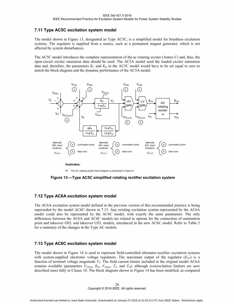
IEEE Std 421.5-2016 IEEE Recommended Practice for Excitation System Models for Power System Stability Studies
7.11 Type AC5C excitation system model
The model shown in Figure 13, designated as Type AC5C, is a simplified model for brushless excitation systems. The regulator is supplied from a source, such as a permanent magnet generator, which is not affected by system disturbances.
The AC5C model introduces the complete representation of the ac rotating exciter (Annex C) and, thus, the open-circuit exciter saturation data should be used. The AC5A model used the loaded exciter saturation data and, therefore, the parameters KC and KD in the AC5C model would have to be set equal to zero to match the block diagram and the dynamic performance of the AC5A model.
HV gate
bb
VUEL VOEL
LV gate
VAKA
1+sTA
VAmax
VAmin
1+sTF3
1+sTF2
sKF
1+sTF1
footnotes:
(a)
VFE
EFE
IFD
EFDAC rotating exciter
(a)
The AC rotating exciter block diagram is presented in Figure 8
summation pointa
b take-over
alternateOEL input locations
(VOEL)
alternateUEL input locations
(VUEL)
summation pointa
b take-over
alternateSCL input locations
(VSCL)
summation pointa
b take-over
b
VSCLuel
b
VSCLoelVF
ΣVC
VREF
VS
–
VUEL
+
+
+ ++
–
aa
Σ
VSCLsum
a
+
VOEL
Figure 13 —Type AC5C simplified rotating rectifier excitation system
7.12 Type AC6A excitation system model
The AC6A excitation system model defined in the previous version of this recommended practice is being superseded by the model AC6C shown in 7.13. Any existing excitation system represented by the AC6A model could also be represented by the AC6C model, with exactly the same parameters. The only differences between the AC6A and AC6C models are related to options for the connection of summation point and takeover OEL and takeover UEL models, introduced in the new AC6C model. Refer to Table 2 for a summary of the changes in the Type AC models.
7.13 Type AC6C excitation system model
The model shown in Figure 14 is used to represent field-controlled alternator-rectifier excitation systems with system-supplied electronic voltage regulators. The maximum output of the regulator (EFE) is a function of terminal voltage magnitude VT. The field current limiter included in the original model AC6A remains available (parameters VFElim, KH, VHmax, TJ, and TH), although overexcitation limiters are now described more fully in Clause 10. The block diagram shown in Figure 14 has been modified, as compared
26 Copyright © 2016 IEEE. All rights reserved.
Authorized licensed use limited to: Iowa State University. Downloaded on January 07,2018 at 21:03:12 UTC from IEEE Xplore. Restrictions apply.

IEEE Std 421.5-2016 IEEE Recommended Practice for Excitation System Models for Power System Stability Studies
to the AC6A block diagram defined in the previous version of this recommended practice, to include the appropriate connections for summation point and takeover overexcitation limiters and underexcitation limiters. The variable VR in the AC6A model corresponds to the exciter field voltage EFE in the AC6C model.
VT∙EFEmax
VT∙EFEmin
VFELIM
VHmax
0
VFE
EFEΣ
1+sTC
1+sTB
HV gate
bb
VUEL VOEL
LV gate
VAmax
VAmin
+–
1+sTK
1+sTAKA
KH1+sTJ
1+sTHΣ
+
–
IFD
EFDAC rotating exciter
(a)
footnotes:
The AC rotating exciter block diagram is presented in Figure 8(a)
summation pointa
b take-over
alternateOEL input locations
(VOEL)
summation pointa
b take-over
alternateUEL input locations
(VUEL)
summation pointa
b take-over
alternateSCL input locations
(VSCL)
VOELsclVUELscl
b b
ΣVC
VREF
VS
–
VUEL
+
+
+ +
+
aa
Σ+
VSCLsum
a
VOEL
Figure 14 —Type AC6C alternator-rectifier excitation system with non-controlled
rectifier and system supplied electronic voltage regulator
7.14 Type AC7B excitation system model
The AC7B excitation system model defined in the previous version of this recommended practice is now superseded by the model AC7C shown in 7.15. Any existing excitation system represented by the AC7B model could also be represented by the AC7C model. The AC7C model offers different options for the connection of overexcitation and underexcitation limiters, which are not available in the AC7B model. Furthermore, the AC7C model offers a more flexible representation of the power source for the controlled rectifier connected to the field winding of the rotating exciter. Refer to Table 2 for a summary of the changes in the Type AC models.
Due to the new representation of the power source of the controlled rectifier, the AC7C model requires additional parameters, as compared to the AC7B model. Thus, the conversion of existing AC7B data into the new AC7C model would require setting switch SW1 to position “A,” switch SW2 to position “A” and KI = KR = XL = KC1 = θP = 0, and VBmax = 99 pu (large number).
Note that a number of modeling software implementations of the AC7B model requires parameter KP to be set to zero to indicate use of an independent power source. Also note that documentation for some systems shows the product KP × VT to be set to 1 to indicate use of an independent power source. In these cases, when using the AC7C model, the user should select the logic SW1 on position “B,” logic SW2 on position “A,” and set KP = 1, KC1 = KR = 0 and VBmax = 99 pu (large value) in the AC7C model to indicate use of an independent power source.
27 Copyright © 2016 IEEE. All rights reserved.
Authorized licensed use limited to: Iowa State University. Downloaded on January 07,2018 at 21:03:12 UTC from IEEE Xplore. Restrictions apply.

IEEE Std 421.5-2016 IEEE Recommended Practice for Excitation System Models for Power System Stability Studies
7.15 Type AC7C excitation system model
The block diagram of the AC7C model is shown in Figure 15.
These excitation systems consist of an ac alternator with either stationary or rotating rectifiers to produce the dc field requirements, as described in 7.1 and shown in Figure 8. Upgrades to earlier ac excitation systems, which replace only the controls but retain the ac alternator and diode rectifier bridge, have resulted in this new model as shown in Figure 15. Some of the features of this excitation system model include a high bandwidth inner loop regulating generator field voltage or exciter current (KF2, KF1), an instantaneous exciter current limit (VFEmax) to protect the field of the ac alternator, and the PID control structure for the automatic voltage regulator (AVR). An alternative rate feedback loop (KF3, TF) is provided for stabilization if the AVR does not include a derivative term.
This excitation system model is an extension of the AC7B model, including the representation of the power source for the controlled rectifier. The user-selected logic switch SW1 determines if the power source of the controlled rectifier is derived from terminal voltage (position “A”) or is independent of the terminal voltage (position “B”). The function FEX1 is the same function FEX shown in Annex D, but the input to the function IN1 should be the exciter field current VFE instead of the generator field current IFD. In these cases, the user-selected logic switch SW2 should be set to position “A.”
The AC7C model also includes the possibility of representing an exciter that employs self-excitation and the voltage regulator power is derived from the exciter output voltage. In such case, the parameter KR should be nonzero and the user-selected logic switch SW2 should be set to position “B” and the model parameters associated with the calculation of the variable VB should have no impact on the simulation.
The AC7C model could be used to represent any equipment currently represented by the AC7B model, as explained in 7.14.
28 Copyright © 2016 IEEE. All rights reserved.
Authorized licensed use limited to: Iowa State University. Downloaded on January 07,2018 at 21:03:12 UTC from IEEE Xplore. Restrictions apply.

IEEE Std 421.5-2016 IEEE Recommended Practice for Excitation System Models for Power System Stability Studies
(a)
−KL∙V
FE
VA
VS
VF
VR
max
VR
min
SW
2(c
)
HV
ga
teLV
ga
te
KF2
Π
KR
KF1
sKF3
1+sT
F
Σ
LV
gate
VA
max
VA
min
KP
R+
KIR s
+sK
DR
1+sT
DR
KP
A+
KIA s
Σ
++
+Σ
b
F EX
1
VB
max
KP
VB
y
ΠS
W1
(b)
KP=K
P θ
P–
y=|K
P∙V
T+j(K
I+K
P∙X
L)∙I T
|–
––
–– I T V
T–F E
X1=
f(IN
1)I N
1
VFE V
E1
–+
+
HV
ga
te
b
VU
EL
LV
gate
b
VO
EL
c
VU
EL
c
VO
EL
d
VO
EL
A B
I N1=
KC
1V
FE VE
1
A B
VFE
EFE I FD
EFD
AC
ro
tatin
g ex
cite
r(a
)V
OE
Lscl
VU
ELs
cl
cc
VO
ELs
cl
b
VU
ELs
cl
b
ΣV
C
VR
EF
VS
–
VU
EL
VO
EL
+ +
++
+–
aa
Σ+
VS
CLs
um
aa
29 Copyright © 2016 IEEE. All rights reserved.
Authorized licensed use limited to: Iowa State University. Downloaded on January 07,2018 at 21:03:12 UTC from IEEE Xplore. Restrictions apply.

IEEE Std 421.5-2016 IEEE Recommended Practice for Excitation System Models for Power System Stability Studies
summation point OEL (at voltage error)a
b take-over OEL (at voltage error)
footnotes:
SW1 is a user-selection option. Position A corresponds to a power source derived from generator terminal voltage, such as an excitation transformer. Position B corresponds to a power source independent of generator terminal conditions, such as a pilot exciter.
(a)
alternateOEL input locations
(VOEL)c take-over OEL (at voltage regulator output)
d take-over OEL (at output of inner loop regulator)
summation point UEL (at voltage error)a
b take-over UEL (at voltage error)
alternateUEL input locations
(VUEL)c take-over UEL (at voltage regulator output)
voltage error calculationa
b after take-over UEL
alternatePSS input locations
(VS)
(b)
SW2 is a user-selection option. Position A corresponds to a power source from signal VB. Position B corresponds to a power source derived from the rotating exciter output (EFD).
(c)
summation point UEL (at voltage error)a
b take-over UEL (at voltage error)
alternateSCL input locations
(VSCL)c take-over UEL (at voltage regulator output)
The AC rotating exciter block diagram is presented in Figure 8
(b)
Figure 15 —Type AC7C alternator-rectifier excitation system: (a) block diagram, (b) notes and footnotes
7.16 Type AC8B excitation system model
The AC8B excitation system model defined in the 2005 version of this recommended practice is being superseded by the model AC8C shown in 7.16. Any existing excitation system represented by the AC8B model could also be represented by the AC8C model. The AC8C model offers different options for the connection of overexcitation and underexcitation limiters, which are not available in the AC8B model. Furthermore, the AC8C offers a more flexible representation of the power source for the controlled rectifier connected to the rotating exciter field winding. Refer to Table 2 for a summary of the changes in the Type AC models.
Because of the new representation of the power source of the controlled rectifier, the AC8C model requires additional parameters, as compared to the AC8B model. Thus, the conversion of existing AC8B data into the new AC8C model would require setting KI = XL = KC1 = θP = 0, and VBmax = 99 pu (large number). The logic switch SW1 in the AC8C model should be set to position “B,” to represent an independent power source.
7.17 Type AC8C excitation system model
The block diagram of the AC8C model is shown in Figure 16.
The AVR in this model consists of PID control, with separate constants for the proportional (KPR), integral (KIR) and derivative (KDR) gains. The values for the constants are chosen for best performance for each particular generator excitation system. The Type AC8C model can be used to represent static voltage regulators applied to brushless excitation systems. Digitally based voltage regulators feeding dc rotating main exciters could also be represented with the AC8C model with the parameters KC and KD set to zero.
This excitation system model is an extension of the AC8B model to include the representation of the power source for the controlled rectifier, as well as accounting for the rectifier loading and commutation effects as described in Annex D. The user-selected logic switch SW1 determines if the power source of the controlled
30 Copyright © 2016 IEEE. All rights reserved.
Authorized licensed use limited to: Iowa State University. Downloaded on January 07,2018 at 21:03:12 UTC from IEEE Xplore. Restrictions apply.

IEEE Std 421.5-2016 IEEE Recommended Practice for Excitation System Models for Power System Stability Studies
rectifier is derived from terminal voltage (position “A”) or is independent of the terminal voltage (position “B”). The function FEX1 is the same function FEX shown in Annex D, but the input to the function IN1 should be the exciter field current VFE instead of the generator field current IFD.
The AC8C model could be used to represent any equipment currently represented by the AC8B model, as explained in 7.16.
(a)
F EX
1
VB
max
KP
VB
y
ΠS
W1
(b)
KP=K
P θ
P–
y=|K
P∙V
T+j(K
I+K
P∙X
L)∙I T
|–
––
–
VFE
Π
VP
IDm
ax
VP
IDm
in
HV
ga
te
cc
VU
EL
VO
EL
LV
gate
KP
R+
KIR s
+sK
DR
1+sT
DR
KA
1+sT
A
VR
max
VR
min
VR
b
VO
EL
LV
gate
VS
Σ
b
HV
ga
te
b
VU
EL
++
– I T VT–
F EX
1=f(I
N1)
I N1
VFE V
E1
A B
I N1=
KC
1V
FE VE
1
EFE
I FD
AC
ro
tatin
g ex
cite
r(a
)
EFD
VO
ELs
clV
UE
Lscl
cc
VO
ELs
clV
UE
Lscl
bb
Σ–
+
+ +
VR
EF
VC
a
VU
EL
a
VO
EL
VS
CLs
um
a
+
31 Copyright © 2016 IEEE. All rights reserved.
Authorized licensed use limited to: Iowa State University. Downloaded on January 07,2018 at 21:03:12 UTC from IEEE Xplore. Restrictions apply.

IEEE Std 421.5-2016 IEEE Recommended Practice for Excitation System Models for Power System Stability Studies
footnotes:
SW1 is a user-selection option. Position A corresponds to a power source derived from generator terminal voltage, such as an excitation transformer. Position B corresponds to a power source independent of generator terminal conditions, such as a pilot exciter.
(a)
(b)
The AC rotating exciter block diagram is presented in Figure 8
summation point (at voltage error)a
b take-over (at voltage error)
alternateUEL input locations
(VUEL)c take-over (at voltage regulator output)
voltage error calculationa
b after take-over UEL
alternatePSS input locations
(VS)
summation point (at voltage error)a
b take-over (at voltage error)
alternateSCL input locations
(VSCL)c take-over (at voltage regulator output)
summation point (at voltage error)a
b take-over (at voltage error)
alternateOEL input locations
(VOEL)c take-over (at voltage regulator output)
(b)
Figure 16 —Type AC8C alternator-rectifier excitation system: (a) block diagram, (b) notes and footnotes
7.18 Type AC9C excitation system model
The block diagram of the excitation system AC9C is shown in Figure 17. The AC9C model may be applied to excitation systems consisting of an ac alternator with either stationary or rotating rectifiers (Glaninger-Katschnig, Nowak, Bachle, and Taborda [B16]). The user-selected logic switch SW1 determines if the power source of the controlled rectifier is derived from terminal voltage and current (position “A”) or is independent of the terminal voltage (position “B”). The function FEX1 is the same function FEX shown in Annex D, but the input to the functions IN1 and IN2 should be the exciter field current VFE instead of the generator field current IFD. Depending on the actual implementation of the potential and current source, the contribution factor is either multiplied or summed to the power stage output.
The model consists of a PID type voltage regulator followed by a PI current regulator in cascade. The model is based on IEC 60034-16-1991 [B19] Part 2 E.5. Both regulator blocks have non-windup limits. The compensated terminal voltage VC (see Figure 2), the power system stabilizer (PSS) output signal VS, and the voltage reference value VREF are applied to the summing point at the input to the voltage regulator. The limiter signals, from the overexcitation limiter VOEL and the underexcitation limiter VUEL, are typically summed into the input of the current regulator.
The power stage control characteristic is represented by the gain KA. The time constant TA represents the time delay caused by the gate control unit and the power stage. The power stage consists either of a thyristor converter bridge or a chopper converter.
The parameter SCT is provided to allow the selection of the power stage type, either a thyristor or a chopper converter. In the logic shown in Figure 17, if the parameter SCT is different than 0, it represents a thyristor converter. When the parameter SCT is set to 0 it represents a chopper converter, and the negative voltage field forcing limit is dependent on the free wheel factor KFW.
32 Copyright © 2016 IEEE. All rights reserved.
Authorized licensed use limited to: Iowa State University. Downloaded on January 07,2018 at 21:03:12 UTC from IEEE Xplore. Restrictions apply.

IEEE Std 421.5-2016 IEEE Recommended Practice for Excitation System Models for Power System Stability Studies
The free wheel factor KFW can be calculated as in Equation (4):
FWFW
Fag
RKR
= (4)
where
RFW is the free-wheel resistor in ohms
RFag is the exciter air-gap field resistance, at a defined reference temperature, in ohms
The exciter air-gap field resistance is derived from the exciter air-gap field current and exciter air-gap field voltage.
The user-selected logic switch SW1 determines if the power source of the controlled rectifier is derived from terminal voltage and current (position “A”) or is independent of the terminal voltage (position “B”). The functions FEX1 and FEX2 are the same as function FEX shown in Annex D. The input to the functions IN1 and IN2 is the exciter field current VFE instead of the generator field current IFD.
Depending on the actual implementation of the potential and current source, the contribution factor is either multiplied or summed to the power stage output. The summation component (VB2) corresponds to a compound power source derived from generator terminal current via a separate series diode bridge. It can be disabled by setting the parameter KI2 equal to zero. The lower limit applied to the signal VI was introduced to prevent a possible division by zero in the calculation of IN2. There are at least two possibilities that could lead to such division by zero: the parameter KI2 is equal to zero or the simulation corresponds to an open-circuit condition, so IT = 0.
33 Copyright © 2016 IEEE. All rights reserved.
Authorized licensed use limited to: Iowa State University. Downloaded on January 07,2018 at 21:03:12 UTC from IEEE Xplore. Restrictions apply.

IEEE Std 421.5-2016 IEEE Recommended Practice for Excitation System Models for Power System Stability Studies
(a)
pow
er
stag
e lo
gic
(d)
0.00
1
VFE
EFE
Σ
ΠV
PID
max
VP
IDm
inH
V
gate
bbVU
EL
VO
EL LV
ga
te
KP
R+
KIR s
+sK
DR
1+sT
DR
KA
1+sT
A
VR
max
VR
min
VR
Σ
KFW
VA
max
VA
min
KP
A+
KIA s
VA
VR
VF
I FD
ref
VC
T
VFW
VFW
max
VFW
min
++
VI=
|KI2∙I T
|–
–+
ΣV
C
VR
EF VS
–
VU
EL
+
++
aa
VO
EL
KF
1+sT
F
VB
2max V
B2
(c)
F EX
2=f(I
N2)
F EX
2
I N2
Π
VFE
VII N
2=K
C2V
FE VI
F EX
1
VB
1max
KP
VB
1
y
ΠS
W1
(b)
KP=K
P θ
P–
y=|K
P∙V
T+j(K
I+K
P∙X
L)∙I T
|–
––
–
– I T VT–
F EX
1=f(I
N1)
I N1
VFE V
E1
b
VS
CLu
el
b
VS
CLo
el
Σ
+
VS
CLs
um
a
+
+
I FD
EFD
AC
ro
tatin
g ex
cite
r(a
)
A B
I N1=
KC
1V
FE VE
1
34 Copyright © 2016 IEEE. All rights reserved.
Authorized licensed use limited to: Iowa State University. Downloaded on January 07,2018 at 21:03:12 UTC from IEEE Xplore. Restrictions apply.

IEEE Std 421.5-2016 IEEE Recommended Practice for Excitation System Models for Power System Stability Studies
IF SCT ≠ 0 (this represents a thyristor bridge)VR = VCT
ELSE (this represents a chopper converter) IF VAVR > Vlim1 VR = VCT ELSE IF VAVR > Vlim2 VR = 0 ELSE VR = −VFW ENDIF ENDIFENDIF
summation point a
b take-over
a
b
alternateOEL input locations
(VOEL)
alternateUEL input locations
(VUEL)
summation point
take-over
footnotes:
SW1 is a user-selection option. Position A corresponds to a power source derived from generator terminal voltage, such as an excitation transformer. Position B corresponds to a power source independent of generator terminal conditions, such as a pilot exciter.
(b)
This portion of the power source requires a special excitation transformer and an additional rectifier bridge, so it should be considered a special application. This portion of the model can be disabled by setting KI2 and KC2 equal to zero.
(c)
The power stage logic uses user-selected parameters SCT, Vlim1 and Vlim2, and the signals VCT, VFW and VAVR shown in the block diagram. The parameter Vlim1 should be greater than Vlim2. Typical values are Vlim1=0 and Vlim2=−0.1 pu.
(d)
summation point a
b take-over
alternateSCL input locations
(VSCL)
The AC rotating exciter block diagram is presented in Figure 8(a)
(b)
Figure 17 —Type AC9C alternator-rectifier excitation system: (a) block digram, (b) notes and footnotes
7.19 Type AC10C excitation system model
The block diagram of the excitation system of Type AC10C shown in Figure 18 represents an excitation system with a brushless exciter, which is fed from an independent source or is supplied via the generator terminals. The user-selected logic switch SW1 determines if the power source of the controlled rectifier is derived from terminal voltage and current (position “A”) or is independent of the terminal voltage (position “B”). The functions FEX1 and FEX2 are the same function FEX shown in Annex D, but the input to the functions IN1 and IN2 should be the exciter field current VFE instead of the generator field current IFD. The model additionally offers the capability of representing an additive component of the power source (added to the exciter field voltage) derived from the generator terminal current.
The model offers a common gain factor KR and two lead-lag elements for the AVR as well as for the underexcitation and overexcitation limiters with independent control settings when a limiter is active, realized by the parallel configuration of lead-lag blocks. The appropriate control path is activated by the logic switches SWUEL and SWOEL, but exclusively when the VUEL and/or VOEL signals are connected to their respective alternate positions “B.” The UEL is considered active for the logic switch SWUEL when the output of the high-value (HV) gate associated with the UEL input alternate position “B” is equal to VUEL. Similarly, the logic switch SWOEL considers the OEL active when the output of the low-value (LV) gate associated with the OEL input alternate position “B” is equal to VOEL. The model additionally offers alternate input positions for stator current limiter VSCL. It should be noted that the logic switches SWUEL and SWOEL are not affected by the SCL signal, even when the SCL signal is connected to its alternate position “B.”
The control signal VR1 is either directly controlling the power stage or serves as reference for a cascaded exciter field current VFE control loop (see Figure 19). This current control subsystem is bypassed when the logic switch SWSS is selected to position “A” (i.e., when gains KCR and KLIM are set equal to zero) and is active when switch SWSS is on position “B.” The current control subsystem also offers a limiter, which avoids overloads of the exciter machine and limits the exciter current to VFELIM. This exciter field current limiter is active when the logic switch SWLIM is set to position “B” (i.e., when gain KLIM is greater than zero), and the limiter is bypassed when SWLIM is set to position “A.” The switch SWEXC allows the choice of the feedback variable, either the generator field voltage EFD (on those implementations where this signal is
35 Copyright © 2016 IEEE. All rights reserved.
Authorized licensed use limited to: Iowa State University. Downloaded on January 07,2018 at 21:03:12 UTC from IEEE Xplore. Restrictions apply.

IEEE Std 421.5-2016 IEEE Recommended Practice for Excitation System Models for Power System Stability Studies
available). On brushless units, the feedback should be from VFE (proportional to exciter field current) as the generator field quantities are not available for measurement.
The model offers configurable inputs for the stabilizer (VS). The stabilizer signal can be added to the summing junction (voltage or limiter reference), or to the output of the gate-structure via separate, but identical control elements.
The limiters (signals VUEL, VOEL, and VSCL) could be summation type (at the voltage reference) and/or takeover action. The type of action for the limiters is selected independently of each other.
The representation of the brushless exciter is equivalent to the model described in 7.1 and shown in Figure 8.
36 Copyright © 2016 IEEE. All rights reserved.
Authorized licensed use limited to: Iowa State University. Downloaded on January 07,2018 at 21:03:12 UTC from IEEE Xplore. Restrictions apply.

IEEE Std 421.5-2016 IEEE Recommended Practice for Excitation System Models for Power System Stability Studies
(a)
curr
ent
cont
rol
subs
yste
m(f)
VFE
EFE
I FD
ΣV
R2
++
Π
0.00
1
VI=
|KI2∙I T
|–
VB
1
VB
1max
VB
2max V
B2
(c)
F EX
2=f(I
N2)
F EX
2
I N2
Π
VFE
VII N
2=K
C2V
FE VI
VR
1
EFD
ΣK
RVR
max
VR
min
KRVR
Sm
ax
VR
Sm
inV
RS
min/K
R
1+sT
C1
1+sT
B1
VR
Sm
ax/K
R
1+sT
C2
1+sT
B2
ΣSW
OE
L(e
)
SW
UE
L(d
)
VR
min/K
R
1+sT
C1
1+sT
B1
VR
max
/KR
1+sT
C2
1+sT
B2
VR
min/K
R
VR
max
/KR
1+sT
UC
2
1+sT
UB
2
1+sT
UC
1
1+sT
UB
1 VR
min/K
R
VR
max
/KR
1+sT
OC
2
1+sT
OB
2
1+sT
OC
1
1+sT
OB
1
Σ
+
++
aVS
+
SW
LIM
Logi
c(k
)
++
+
cVS
bVS
VS
2
VS
1
HV
ga
te
c
VU
EL
LV
gate
c
VO
EL
(j)
(j)
(g)
(g)
(h)
(h)
(i)
(i)
EFD
AC
ro
tatin
g ex
cite
r(a
)
F EX
1
VFE
VE
1S
W1
(b)
KP
yy=
|KP∙V
T+j(K
I+K
P∙X
L)∙I T
|–
––
–
VT–
KP=K
P θ
P–
I T–
A B
F EX
1=f(I
N1)
I N1
Π
A B
A B
Σ–
+
+ +
VR
EF
VC
HV
ga
te
b
VU
EL
LV
gate
b
VO
EL
a
VU
EL
a
VO
EL
VS
CLs
um
a
+
b
VS
CLu
el
b
VS
CLo
el
c
VS
CLu
el
c
VS
CLo
el
I N1=
KC
1V
FE VE
1
37 Copyright © 2016 IEEE. All rights reserved.
Authorized licensed use limited to: Iowa State University. Downloaded on January 07,2018 at 21:03:12 UTC from IEEE Xplore. Restrictions apply.

IEEE Std 421.5-2016 IEEE Recommended Practice for Excitation System Models for Power System Stability Studies
footnotes:
SW1 is a user-selection option. Position A corresponds to a power source derived from generator terminal voltage, such as an excitation transformer. Position B corresponds to a power source independent of generator terminal conditions, such as a pilot exciter.
(a)(b)
(c) This portion of the power source requires a special excitation transformer and an additional rectifier bridge, so it should be considered a special application. This portion of the model can be disabled by setting KI2 and KC2 equal to zero.
(d)
(e)
(f) The current control subsystem uses the signals VR1, EFD and VFE shown in the block diagram. The current control subsystem is fully described in Figure 19.
(g) The upper and lower limits for the block are calculated based on other model parameters: the gain KR, the time constants TB1 and TC1, and the limits VRmax and VRmin.
Vmax=(VRmax−VRmin) TB1
KR TC1
=−Vmin
(h) The upper and lower limits for the block are calculated based on other model parameters: the gain KR, the time constants TUB1 and TUC1, and the limits VRmax and VRmin.
Vmax=(VRmax−VRmin) TUB1
KR TUC1
=−Vmin
(i) The upper and lower limits for the block are calculated based on other model parameters: the gain KR, the time constants TOB1 and TOC1, and the limits VRmax and VRmin.
Vmax=(VRmax−VRmin) TOB1
KR TOC1
=−Vmin
(j) The upper and lower limits for the block are calculated based on other model parameters: the gain KR, the time constants TB1 and TC1, and the limits VRSmax and VRSmin.
Vmax=(VRSmax−VRSmin) TB1
KR TC1
=−Vmin
The AC rotating exciter block diagram is presented in Figure 8
summation point (at voltage error)a
b take-over (at voltage error)
alternateOEL input locations
(VOEL)c take-over (at voltage regulator output)
summation point (at voltage error)a
b take-over (at voltage error)
alternateUEL input locations
(VUEL)c take-over (at voltage regulator output)
voltage error calculationa
b Voltage error or after take-over limits
alternatePSS input locations
(VS)c Output of AVR (after take-over limits)
summation point (at voltage error)a
b take-over (at voltage error)
alternateSCL input locations
(VSCL)c take-over (at voltage regulator output)
IF OEL or UEL are activeVS1 = 0VS2 =VS
ELSEVS1 = VSVS2 = 0
ENDIF
(k) The SWLIM logic described below is only applicable if the alternate PSS input location “B” has been selected, otherwise VS1 = VS2 = 0.
Position B is active when the UEL input location “B” is selected and the UEL is active. Position A is used, otherwise.Position B is active when the OEL input location “B” is selected and the OEL is active. Position A is used, otherwise.
(b)
Figure 18 —Type AC10C alternator-rectifier excitation system: (a) block diagram, (b) notes and footnotes
38 Copyright © 2016 IEEE. All rights reserved.
Authorized licensed use limited to: Iowa State University. Downloaded on January 07,2018 at 21:03:12 UTC from IEEE Xplore. Restrictions apply.

IEEE Std 421.5-2016 IEEE Recommended Practice for Excitation System Models for Power System Stability Studies
current control subsystem
–
VR1
EFD
LV gate
VRmax
VRmin+
KEXC
SWEXC(a)VFE
1+sTF1
1+sTF21
1+sTEXC
Σ KCR
SWKCR(c)
SWSS(d)
SWLIM(b)
VRmax
KLIMΣKVFE
VFELIM
–+
VRmax
VRmin
VR2
footnotes:
Position B of the SWLIM logic switch is selected if the parameter KLIM is non-zero. If KLIM=0, position A is selected.
User-selection option. Position A corresponds to feedback from generator field voltage (EFD) and position B corresponds to feedback from exciter field current (VFE).
(a)
(b)Position B of the SWKCR logic switch is selected if the parameter KCR is non-zero. If KCR=0, position A is selected.(c)Position B of the SWSS logic switch is selected if (KCR+KLIM) > 0. Otherwise, position A is selected.(d)
A
B
A
B
A
B
A
B
VRmax
VRmin
1
1+sTEXC
Figure 19 —Current control subsystem for Type AC10C excitation system model
7.20 Type AC11C excitation system model
The block diagram of the AC11C excitation system model is shown in Figure 20. This model is used to represent a brushless excitation system which is supplied from the generator’s terminals or from a power source independent of the generator (e.g., a permanent magnet generator or a power supply considered independent from the generator terminal conditions). Additionally it offers a selection of compound circuits, which is added to the exciter field voltage. This additive circuit can be selected as a boost circuit, applied when faulted conditions in the system has caused a drop in the terminal voltage of the generator (VT < VBoost). The circuit is released as soon as the generator voltage recovers. The additive component can be permanently added, if VBoost is set to a high value, such as 2 pu. This logic associated with the boost circuit is represented in the block diagram of Figure 20 by the logic switch SWBoost. If terminal voltage is greater than the threshold VBoost (VT > VBoost), SWBoost is set to position “A,” otherwise SWBoost is set to position “B.”
In this model the input for the power system stabilizer (VS) can be connected at different locations, namely at the summing point or at the output of the AVR. This option allows the PSS to remain in service even when the limiter signals (VUEL, VOEL, and VSCL) are connected at the input of the AVR, either as summation point limiters or take-over limiters.
The AVR controller is a PID control structure. Activation of a limiter causes an immediate change of the AVR transfer function to the controller path which corresponds to the activated limiter. The UEL is considered active for the logic switch SWUEL when the output of the HV gate associated with the UEL input alternate position “B” is equal to VUEL. Similarly, the logic switch SWOEL considers the OEL active when the output of the LV gate associated with the OEL input alternate position “B” is equal to VOEL. The model additionally offers alternate input positions for stator current limiter (VSCL). It should be noted that the logic switches SWUEL and SWOEL are not affected by the SCL signal, even when the SCL signal is connected to its alternate position “B.”
It should be noted that this automatic transfer is only applicable when the UEL and/or OEL alternate input location “B” is selected, otherwise the logic switches SWUEL and SWOEL would remain in position “A.” These logic switches are also independent of the SCL limiter, even if the SCL alternate input location “B” is selected.
39 Copyright © 2016 IEEE. All rights reserved.
Authorized licensed use limited to: Iowa State University. Downloaded on January 07,2018 at 21:03:12 UTC from IEEE Xplore. Restrictions apply.

IEEE Std 421.5-2016 IEEE Recommended Practice for Excitation System Models for Power System Stability Studies
(a)
Σ+
+
ΠH
V
gate
c
VU
EL
LV
gate
VA
max
VA
min
c
VO
EL
+Σ
+
VR
Sm
ax
VR
Sm
in
Σ
SW
OE
L(e
)
VR
max
VR
min
SW
UE
L(d
)
VR
max
VR
min
VR
max
VR
min
Σ
+
aVS
+
SW
LIM
Logi
c(f)
++
+
cVS
bVS
VS
2
VS
1
1+sK
BT B
KB+s
T B)
(K
PA+
KP
A
sTIA)
(
1+sK
BT B
KB+s
T B)
(K
PU+
KP
U
sTIU)
(
1+sK
BT B
KB+s
T B)
(K
PA+
KP
A
sTIA)
(
0.00
1
VI=
|KI2∙I T
|–
VB
1
VB
1max
VB
2max
VB
2
F EX
2=f(I
N2)
F EX
2
I N2
Π
VFE
VI
I N2=
KC
2V
FE VI
F EX
1
VFE
VE
1S
W1
(b)
KP
yy=
|KP∙V
T+j(K
I+K
P∙X
L)∙I T
|–
––
–
VT–
KP=K
P θ
P–
I T–
A B
F EX
1=f(I
N1)
I N1
Π
Σ–
+
+ +
VR
EF
VC
HV
ga
te
b
VU
EL
LV
gate
b
VO
EL
a
VU
EL
a
VO
EL
VS
CLs
um
a
+
b
VS
CLu
el
b
VS
CLo
el
Σ+
+
KB
oost
A B
SW
boos
t(c
)
0
A BA B
VFE
EFE
I FD
EFD
AC
ro
tatin
g ex
cite
r(a
)
c
VS
CLu
el
c
VS
CLo
el
I N1=
KC
1V
FE VE
1
KP
O+
KP
O
sTIO
40 Copyright © 2016 IEEE. All rights reserved.
Authorized licensed use limited to: Iowa State University. Downloaded on January 07,2018 at 21:03:12 UTC from IEEE Xplore. Restrictions apply.

IEEE Std 421.5-2016 IEEE Recommended Practice for Excitation System Models for Power System Stability Studies
footnotes:
SW1 is a user-selection option. Position A corresponds to a power source derived from generator terminal voltage, such as an excitation transformer. Position B corresponds to a power source independent of generator terminal conditions, such as a pilot exciter.
(a)
(b)
(c)
(d)
(f)
summation point (at voltage error)a
b take-over (at voltage error)
alternateOEL input locations
(VOEL)c take-over (at voltage regulator output)
summation point (at voltage error)a
b take-over (at voltage error)
alternateUEL input locations
(VUEL)c take-over (at voltage regulator output)
voltage error calculationa
b Voltage error or after take-over limits
alternatePSS input locations
(VS)c Output of AVR (after take-over limits)
summation point (at voltage error)a
b take-over (at voltage error)
alternateSCL input locations
(VSCL)c take-over (at voltage regulator output)
The AC rotating exciter block diagram is presented in Figure 8
The logic switch SWboost depends on the user-selected parameter Vboost. SWboost is in position A (boost source disabled) if VT > Vboost. Otherwise in position B (boost source enabled). This voltage boost feature is essentially disabled when Vboost is set equal to zero.
IF OEL or UEL are activeVS1 = 0VS2 =VS
ELSEVS1 = VSVS2 = 0
ENDIF
The SWLIM logic described below is only applicable if the alternate PSS input location “B” has been selected, otherwise VS1 = VS2 = 0.
(e)
Position B is active when the UEL input location “B” is selected and the UEL is active. Position A is used, otherwise.
Position B is active when the OEL input location “B” is selected and the OEL is active. Position A is used, otherwise.
(b)
Figure 20 —Type AC11C alternator-rectifier excitation system: (a) block diagram, (b) notes and footnotes
8. Type ST—Static excitation systems
8.1 General
In these excitation systems, voltage (and also current in compounded systems) is transformed to an appropriate level. Rectifiers, either controlled or non-controlled, provide the necessary direct current for the generator field.
While many of these systems allow negative field voltage forcing, most do not supply negative field current. For specialized studies where negative field current should be accommodated, more detailed modeling is required, as discussed in Annex G.
For many of the static systems, exciter ceiling voltage is very high. For such systems, additional field current limiter circuits may be used to protect the exciter and the generator rotor. These frequently include both instantaneous and time-delayed elements, so the models defined in the previous version of this recommended practice have been updated to provide additional flexibility regarding the connection of such limiters. Limiters are now described more fully in Clause 10 and Clause 11 of this document.
Refer to Table 3 for a summary of the changes in the Type ST models.
Sample data for these excitation system models are presented in Annex H.
8.2 Type ST1A excitation system model
The ST1A excitation system model defined in the previous version of this recommended practice is being superseded by the model ST1C shown in 8.3. Any existing excitation system represented by the ST1A
41 Copyright © 2016 IEEE. All rights reserved.
Authorized licensed use limited to: Iowa State University. Downloaded on January 07,2018 at 21:03:12 UTC from IEEE Xplore. Restrictions apply.

IEEE Std 421.5-2016 IEEE Recommended Practice for Excitation System Models for Power System Stability Studies
model could also be represented by the ST1C model, with exactly the same parameters. The only differences between the ST1A and ST1C models are related to additional options for the connection of summation point and takeover OEL models, introduced in the new ST1C model. Refer to Table 3 for a summary of the changes in the Type ST models.
8.3 Type ST1C excitation system model
The block diagram of the Type ST1C potential-source–controlled rectifier excitation system shown in Figure 21 is intended to represent systems in which excitation power is supplied through a transformer from the generator terminals or the unit’s auxiliaries bus, and is regulated by a controlled rectifier. The maximum exciter voltage available from such systems is directly related to the generator terminal voltage (except as noted below).
In this type of system, the inherent exciter time constants are very small, and exciter stabilization may not be required. On the other hand, it may be desirable to reduce the transient gain of these systems for other reasons. The model shown is sufficiently versatile to represent transient gain reduction (Koessler [B31]) implemented either in the forward path (lead-lag block with time constants TB and TC, in which case the feedback gain KF would normally be set to zero), or in the feedback path by suitable choice of rate feedback parameters KF and TF (in which case the lead-lag block should be ignored, either making TB and TC equal to zero, if allowed in the software implementation, or making TB = TC). Voltage regulator gain and any inherent excitation system time constant are represented by KA and TA, respectively.
The time constants of the second lead-lag block, TC1 and TB1, allow for the possibility of representing transient gain increase, in which case TC1 would be greater than TB1.
The way in which the firing angle for the bridge rectifiers is derived affects the input-output relationship, which is assumed to be linear in the model by choice of a simple gain (KA). For many systems a truly linear relationship applies. In a few systems, the bridge relationship is not linearized, leaving this nominally linear gain a sinusoidal function, the amplitude of which may be dependent on the supply voltage. As the gain is normally set very high, a linearization of this characteristic is normally satisfactory for modeling purposes. The representation of the ceiling is the same whether the characteristic is linear or sinusoidal.
In many cases, the internal limits on VI can be neglected. The field voltage limits that are functions of both terminal voltage and synchronous machine field current should be modeled. The representation of the field voltage positive limit as a linear function of synchronous machine field current is possible because operation of the rectifier bridge in such systems is confined to the mode 1 region as described in Annex D. The negative limit would have a similar current-dependent characteristic, but the sign of the term could be either positive or negative depending upon whether constant firing angle or constant extinction angle is chosen for the limit. As field current is normally low under this condition, the term is not included in the model.
As a result of the very high forcing capability of these systems, a field current limiter is sometimes employed to protect the generator rotor and exciter. The limit start setting (threshold) is defined by ILR and the gain is represented by KLR. To permit this limit to be ignored, provision should be made to allow KLR to be set to zero. The field current limiter in the ST1C model should not be used concurrently with an explicit OEL model representing the instantaneous limit. When the explicit OEL model is added, the gain KLR should be set to zero. This document describes overexcitation and underexcitation limiters more fully in Clause 10 and Clause 11 respectively.
While, for the majority of these excitation systems, a fully controlled bridge is employed, the model is also applicable to systems in which only half of the bridge is controlled, in which case the negative field voltage limit is set to zero (VRmin = 0).
42 Copyright © 2016 IEEE. All rights reserved.
Authorized licensed use limited to: Iowa State University. Downloaded on January 07,2018 at 21:03:12 UTC from IEEE Xplore. Restrictions apply.

IEEE Std 421.5-2016 IEEE Recommended Practice for Excitation System Models for Power System Stability Studies
The block diagram shown in Figure 21 has been modified, as compared to the ST1A block diagram defined in the previous version of this recommended practice, to include the appropriate connections for summation point or takeover overexcitation limiters. Refer to Table 3 for a summary of the changes in the Type ST models.
Figure 21 —Type ST1C potential source–controlled rectifier exciter
VIm
ax
VIm
in
+
VA
max
VA
min
Σ
KLR
VA
KA
1+sT
A
1+sT
C
1+sT
B
1+sT
C1
1+sT
B1
VI
sKF
1+sT
F
–
0
Σ+
–
I FD
I LR
EFD
VT∙
VR
min
VT∙
VR
max
−KC∙I F
D
+ VS b
sum
mat
ion
poin
t UE
L (a
t vol
tage
err
or)
a bta
ke-o
ver U
EL
(at v
olta
ge e
rror
)
alte
rnat
eU
EL
inpu
t lo
catio
ns
(VU
EL)
cta
ke-o
ver U
EL
(at v
olta
ge re
gula
tor o
utpu
t)
volta
ge e
rror
cal
cula
tion
a bsu
mm
atio
n po
int a
t vol
tage
regu
lato
r out
put
alte
rnat
eP
SS
inpu
t lo
catio
ns
(VS)
sum
mat
ion
poin
t OE
L (a
t vol
tage
err
or)
a bta
ke-o
ver O
EL
(at v
olta
ge e
rror
)
alte
rnat
eO
EL
inpu
t lo
catio
ns
(VO
EL)
cta
ke-o
ver O
EL
(at v
olta
ge re
gula
tor o
utpu
t)
VF
HV
ga
te
b
VU
EL b
VS
CLu
el
LV
gate
b
VO
EL b
VS
CLo
el
Σ
–
++
Σ–
+
+
VS
+
a
VU
EL
a
VO
EL
VR
EF
VC V
SC
Lsum
a
+H
V
gate
c
LV
gate
c
VU
EL
VO
EL
c
VS
CLu
el
c
VS
CLo
el
sum
mat
ion
poin
t (vo
ltage
err
or)
a b
alte
rnat
eS
CL
inpu
t lo
catio
ns
(VS
CL)
take
-ove
r at v
olta
ge re
gula
tor i
nput
cta
ke-o
ver a
t inn
er-lo
op o
utpu
t
43 Copyright © 2016 IEEE. All rights reserved.
Authorized licensed use limited to: Iowa State University. Downloaded on January 07,2018 at 21:03:12 UTC from IEEE Xplore. Restrictions apply.

IEEE Std 421.5-2016 IEEE Recommended Practice for Excitation System Models for Power System Stability Studies
8.4 Type ST2A excitation system model
The ST2A excitation system model defined in the previous version of this recommended practice is being superseded by the model ST2C shown in 8.5. Any existing excitation system represented by the ST2A model could also be represented by the ST2C model, with practically the same parameters. The differences between the ST2A and ST2C models are related to additional options for the connection of summation point and takeover OEL models, introduced in the new ST2C model, the addition of parameters VBmax and XL in the representation of the power source for the excitation system, and the introduction of a PI control block in the AVR transfer function. Refer to Table 3 for a summary of the changes in the Type ST models.
The conversion of data from an existing ST2A model to the new ST2C model requires setting XL = 0, KPR = 1, KIR = 0, and defining VPImax = VBmax = 99 pu (large number) and VPImin = –99 pu (large negative number).
8.5 Type ST2C excitation system model
Some static systems utilize both current and voltage sources (generator terminal quantities) to comprise the power source. These compound-source rectifier excitation systems are designated type ST2C and are modeled as shown in Figure 22. It is necessary to form a model of the exciter power source utilizing a phasor combination of terminal voltage (VT) and terminal current IT. Rectifier loading and commutation effects are accounted for as described in Annex D. The parameter EFDmax represents the limit on the exciter voltage due to saturation of the magnetic components. The regulator controls the exciter output through controlled saturation of the power transformer components. The time constant TE is associated with the inductance of the control windings.
The block diagram shown in Figure 22 has been modified, as compared to the ST2A block diagram defined in the previous version of this recommended practice, to include the appropriate connections for summation point or takeover overexcitation limiters, additional parameters in the representation of the power source, making the power source model equal to what is used in other models in this recommended practice, and the addition of a PI control block that would allow the representation of equipment retrofit with a modern digital controller.
44 Copyright © 2016 IEEE. All rights reserved.
Authorized licensed use limited to: Iowa State University. Downloaded on January 07,2018 at 21:03:12 UTC from IEEE Xplore. Restrictions apply.

IEEE Std 421.5-2016 IEEE Recommended Practice for Excitation System Models for Power System Stability Studies
VRmax
VRmin
VRKA
1+sTA
FEX=f(IN)
FEX
IN
ΠKP=KP θP–
–IT
VT–
IFD
VB
VBmax
VE
Π
IN=KCIFD
VEVE=|KP∙VT+j(KI+KP∙XL)∙IT|– – ––
sKF
1+sTF
Σ
–
++
Σ–
+
+
VS
+
a
VUEL
a
VOEL
VREF
VC
VF
+
EFDΣ
1
sTE
EFDmax
KE
–
0
alternateOEL input locations
(VOEL)
alternateUEL input locations
(VUEL)
VPImax
VPImin
KPR+KIR
s
summation point (voltage error)a
b
alternateSCL input locations
(VSCL)take-over at voltage regulator input
HV gate
b
VUEL
b
VSCLuel
LV gate
b
VOEL
b
VSCLoel
VSCLsum
a
+
summation point (voltage error)a
b take-over at voltage regulator input
summation point (voltage error)a
b take-over at voltage regulator input
Figure 22 —Type ST2C compound-source rectifier exciter
8.6 Type ST3A excitation system model
The ST3A excitation system model defined in the previous version of this recommended practice is being superseded by the model ST3C shown in 8.7. Any existing excitation system represented by the ST3A model could also be represented by the ST3C model, with practically the same parameters.
The major differences between the ST3A and ST3C models are related to additional options for the connection of summation point and takeover OEL models, introduced in the new ST3C model, and the addition of a PI control block in the AVR transfer function. Refer to Table 3 for a summary of the changes in the Type ST models.
Additionally, the block representing the dynamic response of the controlled rectifier bridge has been moved to the output of the ST3C model. This might result in differences in the dynamic response of the model, if the feedback gain KG is different than zero.
The conversion of data from an existing ST3A model to the new ST3C model requires setting KPR = 1, KIR = 0, and defining VPImax = 99 pu (large number) and VPImin = –99 pu (large negative number).
45 Copyright © 2016 IEEE. All rights reserved.
Authorized licensed use limited to: Iowa State University. Downloaded on January 07,2018 at 21:03:12 UTC from IEEE Xplore. Restrictions apply.

IEEE Std 421.5-2016 IEEE Recommended Practice for Excitation System Models for Power System Stability Studies
8.7 Type ST3C excitation system model
Some static systems utilize a field voltage control loop to linearize the exciter control characteristic as shown in Figure 23. This also makes the output independent of supply source variations until supply limitations are reached.
These systems utilize a variety of controlled rectifier designs: full thyristor complements or hybrid bridges in either series or shunt configurations. The power source may consist of only a potential source, either fed from the machine terminals or from internal windings. Some designs may have compound power sources utilizing both machine potential and current. These power sources are represented as phasor combinations of machine terminal current and voltage and are accommodated by suitable parameters in the model shown.
VRmax
VRmin
VR
FEX=f(IN)
FEX
IN
Π
KP=KP θP–
–IT
VT–
IFD
VB
VBmax
VE
Π
IN=KCIFD
VE
VPImax
VPImin
KPR+KIR
sKA
1+sTC
1+sTB
KM
1+sTM
KG
VGmax
VMmax
VMmin
SW1(a)
KP
EFD
–+
Σ
VImax
VImin
VM
yy=|KP∙VT+j(KI+KP∙XL)∙IT|
– – ––
footnotes:
SW1 is a user-selection option. Position A corresponds to a power source derived from generator terminal voltage, such as an excitation transformer. Position B corresponds to a power source independent of generator terminal conditions, such as a pilot exciter.
(a)
HV gate
b
VUEL
Σ
++
a a
VS
+
VOEL VUEL
a
Σ–
+
+
VC
VREF
+
VSCLsum
a b
VSCLuel
LV gate
b
VOEL
b
VSCLoel
A
B
alternateOEL input locations
(VOEL)
alternateUEL input locations
(VUEL)
summation point (voltage error)a
b
alternateSCL input locations
(VSCL)take-over at voltage regulator input
summation point (voltage error)a
b take-over at voltage regulator input
summation point (voltage error)a
b take-over at voltage regulator input
Figure 23 —Type ST3C potential or compound source–controlled rectifier exciter
with field voltage control loop
The excitation system stabilizer for these systems is provided by a series lag-lead element in the voltage regulator, represented by the time constants TB and TC. The inner loop field voltage regulator is composed of the gains KM and KG and the time constant TM. This loop has a wide bandwidth compared with the upper limit of 3 Hz for the models described in this recommended practice. The time constant TM may be increased for study purposes, eliminating the need for excessively short computing increments while still retaining the required accuracy at 3 Hz. Rectifier loading and commutation effects are accounted for as discussed in Annex D. The limit VBmax is determined by the saturation level of power components.
46 Copyright © 2016 IEEE. All rights reserved.
Authorized licensed use limited to: Iowa State University. Downloaded on January 07,2018 at 21:03:12 UTC from IEEE Xplore. Restrictions apply.

IEEE Std 421.5-2016 IEEE Recommended Practice for Excitation System Models for Power System Stability Studies
The block diagram shown in Figure 23 has been modified, as compared to the ST3A block diagram defined in the previous version of this recommended practice, to include the appropriate connections for summation point or takeover overexcitation limiters.
8.8 Type ST4B excitation system model
The ST4B excitation system model defined in the previous version of this recommended practice is being superseded by the model ST4C shown in 8.9. Any existing excitation system represented by the ST4B model could also be represented by the ST4C model.
The ST4C model has additional options, compared to the ST4B model, for connecting the OEL and UEL signals, allowing the representation of takeover or summation point limiters. The ST4C model also has additional logic to represent excitation systems that have an independent power supply that is not connected to the generator terminals. Refer to Table 3 for a summary of the changes in the Type ST models.
Because of these new features, the ST4C model requires additional parameters, as compared to the ST4B model. Thus, the conversion of existing ST4B data into the new ST4C model would require setting the user-selected logic switch SW1 to position “A.” Additionally, the upper limit VGmax in the feedback loop for the field current regulator in the ST4C model should be set to VGmax = 99 pu (large number), if this upper limit is not represented in the specific ST4B model implementation, and the time constant TG, in the ST4C model, should be set to zero.
8.9 Type ST4C excitation system model
This model is a variation of the Type ST3C model, with a proportional-integral (PI) regulator block replacing the lag-lead regulator characteristic that was in the ST3C model. Both potential and compound source rectifier excitation systems are modeled as shown in Figure 24. The PI regulator blocks have non-windup limits that are represented as described in Annex E.
The description of the rectifier regulation function FEX is presented in Annex D. There is flexibility in the power component model to represent bus fed exciters (KI and XL both equal to zero), compound static systems (XL = 0), and potential and compound source systems where XL is not zero.
The block diagram shown in Figure 24 has been modified, as compared to the ST4B block diagram defined in the previous version of this recommended practice, to include the appropriate connections for summation point or takeover overexcitation limiters and underexcitation limiters and the addition of the time constant TG on the feedback path with gain KG. For compatibility with the ST4B model, the implementation of the ST4C model should allow the time constant TG to be specified as zero, and thus ignored.
Additionally, the block representing the dynamic response of the controlled rectifier was moved to the output of the model, as compared to the block diagram of the ST4B model. It should be noted that this change might result in different dynamic response, compared to the ST4B model, if the feedback gain KG is different than zero.
The ST4C model also includes a modification to the representation of the power stage of the excitation system. Through proper selection of the logic SW1, it is now possible to represent systems where the ac power supply is independent of the terminal voltage of the generator.
Setting SW1 to position “A” corresponds to the ST4B structure, as defined in the previous version of this recommended practice: the generator field voltage is obtained by multiplying the output of the AVR by the terminal bus voltage magnitude VT, representing the power source. Compatibility with the ST4B model would also require setting the parameter KP = 1, and KI = XL = KC = θP = 0.
47 Copyright © 2016 IEEE. All rights reserved.
Authorized licensed use limited to: Iowa State University. Downloaded on January 07,2018 at 21:03:12 UTC from IEEE Xplore. Restrictions apply.

IEEE Std 421.5-2016 IEEE Recommended Practice for Excitation System Models for Power System Stability Studies
When the logic SW1 is set to position “B,” the output is no longer dependent on terminal voltage.
The ST4C model could be used to represent any equipment currently represented by the ST4B model, as explained in 8.8.
VR
FEX=f(IN)
FEX
IN
Π
KP=KP θP–
–IT
VT–
IFD
VB
VBmax
VE
HV gate
b
LV gate
b
VUEL VOEL
Π
IN=KCIFD
VE
VRmax
VRmin
KPR+KIR
s
VGmax
VAmax
VAmin
SW1(a)
KP
EFD
–+
ΣVM
yy=|KP∙VT+j(KI+KP∙XL)∙IT|
– – ––
Σ
+
+
aa
VS
+
VOELVUEL
1
1+sTA
VMmax
VMmin
KPM+KIM
sHV
gate
c
LV gate
c
VUEL VOEL
Σ+
+
VS
ba
KG
1+sTG
Σ–
+
+VC
VREF
+
VSCLsum
a
b
VSCLuel
c
VSCLuel
b
VSCLoel
c
VSCLoel
A
B
footnotes:
SW1 is a user-selection option. Position A corresponds to a power source derived from generator terminal voltage, such as an excitation transformer. Position B corresponds to a power source independent of generator terminal conditions.
(a)
summation point before take-over UELa
b
alternatePSS input locations
(VS) summation point after take-over UEL
summation point (voltage error)a
b
alternateOEL input locations
(VOEL)
take-over at voltage regulator input
c take-over at inner-loop output
summation point (voltage error)a
b
alternateUEL input locations
(VUEL)
take-over at voltage regulator input
c take-over at inner-loop output
summation point (voltage error)a
b
alternateSCL input locations
(VSCL)
take-over at voltage regulator input
c take-over at inner-loop output
Figure 24 —Type ST4C potential, compound, or independent source–controlled
rectifier static exciter
8.10 Type ST5B excitation system model
The ST5B excitation system model defined in the previous version of this recommended practice is being superseded by the model ST5C shown in 8.11. Any existing excitation system represented by the ST5B model could also be represented by the ST5C model, with exactly the same parameters. The only differences between the ST5B and ST5C models are related to additional options for the connection of summation point OEL and UEL models, introduced in the new ST5C model. Refer to Table 3 for a summary of the changes in the Type ST models.
48 Copyright © 2016 IEEE. All rights reserved.
Authorized licensed use limited to: Iowa State University. Downloaded on January 07,2018 at 21:03:12 UTC from IEEE Xplore. Restrictions apply.

IEEE Std 421.5-2016 IEEE Recommended Practice for Excitation System Models for Power System Stability Studies
8.11 Type ST5C excitation system model
The Type ST5C excitation system shown in Figure 25 is a variation of the Type ST1A model, with alternative overexcitation and underexcitation inputs and additional limits.
The block diagram shown in Figure 25 has been modified, as compared to the ST5B block diagram defined in the previous version of this recommended practice, to include the appropriate connections for summation point overexcitation and underexcitation limiters.
ΣKR
VRmax
VRminSWOEL
(b)
SWUEL(a)
VRmin/KR
1+sTC1
1+sTB1
VRmax/KR
1+sTC2
1+sTB2
VRmin/KR
VRmax/KR
1+sTUC2
1+sTUB2
1+sTUC1
1+sTUB1
VRmin/KR
VRmax/KR
1+sTOC2
1+sTOB2
1+sTOC1
1+sTOB1
Σ
++
KC
1
1+sT1
VT∙VRmin
VT∙VRmax
–+
VS
IFD
EFD
footnotes:(a) Position B is selected when the UEL is active. Position A is used, otherwise.(b) Position B is selected when the OEL is active. Position A is used, otherwise.
Σ–
+
+
+
VREF
VC HV gate
b
VUEL
LV gate
b
VOEL
a
VUEL
a
VOEL
VSCLsum
a
+
b
VSCLuel
b
VSCLoel
A
B
A
B
alternateOEL input locations
(VOEL)
alternateUEL input locations
(VUEL)
summation point (voltage error)a
b
alternateSCL input locations
(VSCL)take-over at voltage regulator input
summation point (voltage error)a
b take-over at voltage regulator input
summation point (voltage error)a
b take-over at voltage regulator input
Figure 25 —Type ST5C static potential source excitation system
8.12 Type ST6B excitation system model
The ST6B excitation system model defined in the previous version of this recommended practice is being superseded by the model ST6C shown in 8.13. Any existing excitation system represented by the ST6B model could also be represented by the ST6C model.
The ST6C model introduces new options for the connection of summation point underexcitation limiter and takeover overexcitation limiter. The ST6C model also incorporates a modified model to represent the power source for the controlled rectifier. Refer to Table 3 for a summary of the changes in the Type ST models.
Due to these new features, the ST6C model requires additional parameters, as compared to the ST6B model. Thus, the conversion of existing ST6B data into the new ST6C model would require setting the logic SW1 to position “A” and setting KI = XL = 0. The new time constant TA introduced in the ST6C model should also be set to zero.
49 Copyright © 2016 IEEE. All rights reserved.
Authorized licensed use limited to: Iowa State University. Downloaded on January 07,2018 at 21:03:12 UTC from IEEE Xplore. Restrictions apply.

IEEE Std 421.5-2016 IEEE Recommended Practice for Excitation System Models for Power System Stability Studies
8.13 Type ST6C excitation system model
The automatic voltage regulator (AVR) shown in Figure 26 consists of a PI voltage regulator with an inner loop field voltage regulator and pre-control. The field voltage regulator implements a proportional control. The pre-control and the delay in the feedback circuit increase the dynamic response. If the field voltage regulator is not implemented, the corresponding parameters KFF and KG are set to 0. The signal VM represents the output of the rectifier bridge considering the limits of the power rectifier. The ceiling current limitation is included in this model. The power for the rectifier (VB) may be derived from the generator terminals or from an independent source, depending on the user-selected logic switch SW1.
The block diagram shown in Figure 26 has been modified, as compared to ST6B block diagram defined in the previous version of this recommended practice and revised in the associated corrigendum, to include the appropriate connections for summation point or takeover overexcitation limiters and underexcitation limiters. Additionally, the time constant TA has been introduced, at the output of the model, to allow the representation of the equivalent effect of time delays and/or transducer time constants between the digital controller and the field voltage. For compatibility with the ST6B model, the implementation of the ST6C model should allow the time constant TA to be specified as zero.
Additionally, the upper limit of the PI block with parameters KPA and KIA is either VAmax or the output of the instantaneous field current limiter. This feature allows the voltage control path (AVR path) to track the field current limit when it is active and thus allow a smooth transition back to voltage control if the field current drops below the limit defined by the parameter ILR.
The ST6C model could be used to represent any equipment currently represented by the ST6B model, as described in 8.12.
50 Copyright © 2016 IEEE. All rights reserved.
Authorized licensed use limited to: Iowa State University. Downloaded on January 07,2018 at 21:03:12 UTC from IEEE Xplore. Restrictions apply.

IEEE Std 421.5-2016 IEEE Recommended Practice for Excitation System Models for Power System Stability Studies
(a)
F EX=f
(I N)
F EX
I N
Π
KP=K
P θ
P–
– I T VT–
VB
VB
max
VE
Π
I N=K
CI F
D VE
KP
yy=
|KP∙V
T+j(K
I+K
P∙X
L)∙I T
|–
––
–
VM
max
VM
min
VA
1
1+sT
A
VA
max
VA
min
HV
ga
te
d
LV
gate
d
VU
EL
VO
EL
EFD
LV
gate
VR
max
VR
min
–
+Σ
KLR
KM
KFF
Σ
+
+
+K
PA+
KIA s
VR
min
KC
IΣ
I FD
KG
1+sT
G
–
Σ–
cc V
S
VO
EL
VU
EL
VC
VR
EF
+++
+H
V
gate
b
LV
gate
b
VU
EL
VO
EL
Σ
aa
VO
EL
VU
EL++
+
I LR
LV
gate
VR
VM
VS
CLs
um
a
b
VS
CLu
el
b
VS
CLo
el
d
VS
CLu
el
d
VS
CLo
el
+
VS
CLs
um
c
+
SW
1(a
)
A B
51 Copyright © 2016 IEEE. All rights reserved.
Authorized licensed use limited to: Iowa State University. Downloaded on January 07,2018 at 21:03:12 UTC from IEEE Xplore. Restrictions apply.

IEEE Std 421.5-2016 IEEE Recommended Practice for Excitation System Models for Power System Stability Studies
footnotes:(a) SW1 is a user-selection option. Position A corresponds to a power source derived from generator
terminal voltage, such as an excitation transformer. Position B corresponds to a power source independent of generator terminal conditions, such as a pilot exciter.
alternateOEL input locations
(VOEL)
alternateUEL input locations
(VUEL)
summation point (at voltage error)a
b take-over (at voltage regulator input)alternateSCL input locations
(VSCL)summation point (at AVR input)c
d take-over (at voltage regulator input)
summation point (at voltage error)a
b take-over (at voltage regulator input)
summation point (at AVR input)c
d take-over (at voltage regulator input)
summation point (at voltage error)a
b take-over (at voltage regulator input)
summation point (at AVR input)c
d take-over (at voltage regulator input)
(b)
Figure 26 —Type ST6C static potential and compound source excitation system with field current limiter: (a) block diagram, (b) notes and footnotes
8.14 Type ST7B excitation system model
The ST7B excitation system model defined in the previous version of this recommended practice is being superseded by the model ST7C shown in 8.15. Any existing excitation system represented by the ST7B model could also be represented by the ST7C model with the same parameters, just defining the new parameter TA = 0. Refer to Table 3 for a summary of the changes in the Type ST models.
8.15 Type ST7C excitation system model
The model ST7C in Figure 27 is representative of static potential source excitation systems. In this system, the AVR consists of a proportional-integral (PI) voltage regulator. A phase lead-lag filter in series allows introduction of a derivative function, although this is typically used only with brushless excitation systems. In that case, the regulator is of the PID type. In addition, the terminal voltage channel includes a phase lead-lag filter.
The AVR includes the appropriate inputs at its reference for overexcitation limiter VOEL, underexcitation limiter VUEL, and stator current limiter VSCLsum. These limiters, when they work at voltage reference level, keep the PSS VS in operation. However, the UEL limiter could also be connected to the HV gate acting on the output signal, representing a takeover action. Similarly, the AVR output signal passes through an LV gate that could be used to represent a takeover overexcitation limiter.
All control loops in the diagram, including limitation functions, are built to obtain a non-windup behavior of any integrator (see Annex E).
52 Copyright © 2016 IEEE. All rights reserved.
Authorized licensed use limited to: Iowa State University. Downloaded on January 07,2018 at 21:03:12 UTC from IEEE Xplore. Restrictions apply.

IEEE Std 421.5-2016 IEEE Recommended Practice for Excitation System Models for Power System Stability Studies
(a)
EFD
1
1+sT
A
VT∙
VR
min
VT∙
VR
max
Σ
+a
VU
EL
a
VO
EL
VR
EF
Σ
KIA
1+sT
IA
1+sT
C
1+sT
B
Σ+
HV
ga
teLV
ga
te
KL
KH
Σ
VT∙
VR
max
–
+–
VT∙
VR
min
KP
AΣ
VS
1+sT
G
1+sT
F
VC
++
HV
ga
te
b
LV
gate
b
VU
EL
VO
EL
HV
ga
te
c
LV
gate
c
VU
EL
VO
EL
Vm
in
Vm
ax
+
+–
–+
VFB (a)
53 Copyright © 2016 IEEE. All rights reserved.
Authorized licensed use limited to: Iowa State University. Downloaded on January 07,2018 at 21:03:12 UTC from IEEE Xplore. Restrictions apply.

IEEE Std 421.5-2016 IEEE Recommended Practice for Excitation System Models for Power System Stability Studies
a
b
alternateOEL input locations
(VOEL)c take-over (at voltage regulator output)
summation point (voltage reference setpoint)a
b take-over (at voltage reference)
alternateUEL input locations
(VUEL)c take-over (at voltage regulator output)
summation point (voltage reference setpoint)
take-over (at voltage reference)
summation point (voltage reference setpoint)a
b take-over (at voltage reference)
alternateSCL input locations
(VSCL)c take-over (at voltage regulator output)
footnotes:
The signal VFB is used as an input for the UEL2C model, when that UEL model is applied in conjunction with the ST7C model
(a)
(b)
Figure 27 —Type ST7C static potential source excitation system: (a) block diagram, (b) notes and footnotes
8.16 Type ST8C excitation system model
The static excitation model ST8C is shown in Figure 28. This model has a PI Type voltage regulator followed by a PI current regulator in cascade. Both regulator blocks have non-windup limits, see Glaninger-Katschnig, Nowak, Bachle, and Taborda [B16]. The cascaded AVR model is based on IEC 60034-16-1991 [B19] Part-2 E.5.
The compensated terminal voltage VC (see also Figure 2), the PSS signal VS, and the voltage reference setpoint value VREF, are applied to the summing point at the input to the voltage regulator. The limiter signals, from the overexcitation limiters VOEL and underexcitation limiters VUEL, are typically summed into the input of the current regulator. For a detailed description and clarification on the cascaded AVR structure, see Glaninger-Katschnig, Nowak, Bachle, and Taborda [B16].
The logic switch SW1 determines if the power source of the controlled rectifier is derived from terminal voltage and current (position “A”) or is independent of the terminal voltage (position “B”). The functions FEX1 and FEX2 are the same as function FEX shown in Annex D. The input to the function IN1 and IN2 are calculated based on the generator field current IFD.
Depending on the actual implementation of the potential and current source, the contribution factor is either multiplied or summed to the power stage output. The summation component (VB2) corresponds to a compound power source derived from generator terminal current. The summation component VB2 can be disabled by setting parameters KI2 and KC2 equal to zero. The lower limit applied to the signal VI was introduced to prevent a possible division by zero in the calculation of IN2. There are at least two possibilities that could lead to such division by zero: the parameter KI2 is equal to zero or the simulation corresponds to an open-circuit condition, so IT = 0.
54 Copyright © 2016 IEEE. All rights reserved.
Authorized licensed use limited to: Iowa State University. Downloaded on January 07,2018 at 21:03:12 UTC from IEEE Xplore. Restrictions apply.

IEEE Std 421.5-2016 IEEE Recommended Practice for Excitation System Models for Power System Stability Studies
FEX1=f(IN1)
FEX1
IN1
Π
KP=KP θP–
–IT
VT–
VB1
VB1max
VE
Π
VAmax
VAmin
VRmax
VRmin
SW1(a)
KP
–+
ΣIFDref
yy=|KP∙VT+j(KI+KP∙XL)∙IT|
– – ––
KA
1+sTAΣ
+KPA+
KIA
s
KF
1+sTF
VPImax
VPImin
KPR+KIR
sHV
gate
b
LV gate
b
VUEL VOEL
FEX2=f(IN2)
FEX2
IN2
Π
IFD
VB2
VB2max
VI(b)
0.001
VI=|KI2∙IT|–
IN1=KC1IFD
VE
IN2=KC2IFD
VI
IFD
IFDF
+
summation pointa
b
alternateOEL input locations
(VOEL)take-over
summation pointa
b
alternateUEL input locations
(VUEL)take-over
footnotes:(a) SW1 is a user-selection option. Position A corresponds to a power source derived from generator terminal voltage, such
as an excitation transformer. Position B corresponds to a power source independent of generator terminal conditions, such as a pilot exciter.
(b) This portion of the power source requires a special excitation transformer and an additional rectifier bridge, so it should be considered a special application. This portion of the model can be disabled by setting KI2 and KC2 equal to zero.
EFD
A
B
b
VSCLuel
b
VSCLoel
Σ
++
aa
VS
+
VOELVUEL
Σ–
+
+VC
VREF
+
VSCLsum
a
summation pointa
b
alternateSCL input locations
(VSCL)take-over
Figure 28 —Type ST8C static potential-compound source excitation system
8.17 Type ST9C excitation system model
The static excitation model ST9C is shown in Figure 29. The voltage regulator implements a proportional-integral (PI) control logic.
A differential stage is included in the path of the compensated voltage VC (see Figure 2) and the output of the differential stage is also added to the AVR summing point. This differential stage is intended to provide a faster reaction of the regulator in case of large voltage variations. A dead-band function (+/–ZA) is provided to eliminate the influence of the differential stage for small changes in the compensated voltage VC.
The underexcitation limiter is also a PI regulator with its own proportional gain, but shares the integral path with the AVR. The appropriate integration time constant is selected depending on the error signals of UEL and AVR. The sign of the difference between the AVR error signal and VUEL signal coming from the UEL model indicates whether UEL is active or the AVR is active.
55 Copyright © 2016 IEEE. All rights reserved.
Authorized licensed use limited to: Iowa State University. Downloaded on January 07,2018 at 21:03:12 UTC from IEEE Xplore. Restrictions apply.

IEEE Std 421.5-2016 IEEE Recommended Practice for Excitation System Models for Power System Stability Studies
The power converter stage is represented by a first-order filter with the gain KAS and the time constant TAS. The time constant TAS represents the total delay caused by the gate control unit and power converter. The gain KAS is proportional to the secondary voltage of the power potential transformer that feeds the power converter.
The logic switch SW1 determines if the power source of the controlled rectifier is derived from terminal voltage and current (position “A”) or is independent of the terminal voltage (position “B”). The function FEX is described in Annex D.
Π
–
+HV
gate
b
LV gate
bVUEL
VOEL
+
EFD
FEX=f(IN)
FEX
IN
Π
KP=KP θP–VT
–
IFD
VB
VBmax
VE
IN=KCIFD
VE
SW1(a)
KP
yy=|KP∙VT+j(KI+KP∙XL)∙IT|
– – ––
VRmax
VRmin
KAS
1+sTASΣKA
Σ Σ
Π1
s
+
Σ
1
TA
1
TAUEL ++
KU
Σ+
–
1
0
+–
–
VC
VREF
Σ
a
a
VOEL
VUEL
+
+
+
+
VS
Σ
sTCD
1+sTBD
ZA
−ZA
++
–
1
summation point (voltage error)a
b
alternateOEL input locations
(VOEL)take-over
alternateUEL input locations
(VUEL)
footnotes:(a) SW1 is a user-selection option. Position A corresponds to a power source derived from
generator terminal voltage, such as an excitation transformer. Position B corresponds to a power source independent of generator terminal conditions, such as a pilot exciter.
–IT
A
B
b
VSCLuel b
VSCLoel
+
VSCLsum
a
summation point (voltage error)a
b take-over
alternateSCL input locations
(VSCL)
summation point (voltage error)a
b take-over
Figure 29 —Type ST9C static potential-compound source excitation system
8.18 Type ST10C excitation system model
The static excitation model ST10C is shown in Figure 30. This model is a variation of the ST1C and ST5C models. In addition to ST5C model, this model offers alternatives for the application of the stabilizing signal VS coming from the PSS. It offers the option to apply the PSS signal at the AVR summing junction (voltage reference) and/or at the output of the gate structure, via separate but identical control elements. Furthermore, it offers the flexibility to interconnect the limiter signals VUEL, VOEL, and VSCL at different locations depending on the actual equipment configuration or settings. The ST10C model also offers independent control settings for when a limiter is active, realized by the parallel configuration of lead-lag blocks. The appropriate control path is activated by the logic switches SWUEL and SWOEL, but exclusively when the VUEL and VOEL signals are connected to their respective alternate positions “B.” The UEL is
56 Copyright © 2016 IEEE. All rights reserved.
Authorized licensed use limited to: Iowa State University. Downloaded on January 07,2018 at 21:03:12 UTC from IEEE Xplore. Restrictions apply.

IEEE Std 421.5-2016 IEEE Recommended Practice for Excitation System Models for Power System Stability Studies
considered active for the logic switch SWUEL when the output of the HV gate associated with the UEL input alternate position “B” is equal to VUEL. Similarly, the logic switch SWOEL considers the OEL active when the output of the LV gate associated with the OEL input alternate position “B” is equal to VOEL.
The model additionally offers alternate input positions for stator current limiter (VSCL). It should be noted that the logic switches SWUEL and SWOEL are not affected by the SCL signal, even when the SCL signal is connected to the alternate position “B.”
The logic SWLIM applies to the situation where the PSS is added to the voltage reference error under normal operation conditions, but is switched to the alternate position if one of the takeover limiters (OEL or UEL) becomes active. It should be noted that when the PSS option “B” is selected, the signals VS for the other PSS input options should be considered as zero.
The logic switch SW1 determines if the power source of the controlled rectifier is derived from the terminal voltage and current (position “A”) or is independent of the terminal voltage (position “B”). The function FEX is described in Annex D.
57 Copyright © 2016 IEEE. All rights reserved.
Authorized licensed use limited to: Iowa State University. Downloaded on January 07,2018 at 21:03:12 UTC from IEEE Xplore. Restrictions apply.

IEEE Std 421.5-2016 IEEE Recommended Practice for Excitation System Models for Power System Stability Studies
(a)
ΠE
FDΣ
KRV
Rm
ax
VR
min
KRVR
Sm
ax
VR
Sm
inV
RS
min/K
R
1+sT
C1
1+sT
B1
VR
Sm
ax/K
R
1+sT
C2
1+sT
B2
Σ
SW
OE
L(c
)
SW
UE
L(b
)
VR
min/K
R
1+sT
C1
1+sT
B1
VR
max
/KR
1+sT
C2
1+sT
B2
VR
min/K
R
VR
max
/KR
1+sT
UC
2
1+sT
UB
2
1+sT
UC
1
1+sT
UB
1
VR
min/K
R
VR
max
/KR
1+sT
OC
2
1+sT
OB
2
1+sT
OC
1
1+sT
OB
1
Σ
+
++
aVS
+
SW
LIM
logi
c(h
)
++
+
cVS
bVS
VS
2
VS
1
Σ–
+
+ +
VR
EF
VC
HV
ga
te
b
VU
EL
LV
gate
b
VO
EL
a
VU
EL
a
VO
EL
HV
ga
te
c
VU
EL
LV
gate
c
VO
EL
1
1+sT
1
VR
max
VR
min
(d)
(d)
(e)
(e)
(f)
(f)
(g)
(g)
VS
CLs
um
a
+
b
VS
CLu
el
b
VS
CLo
el
c
VS
CLu
el
c
VS
CLo
el
A B
A B
F EX
I FD
VE
SW
1(a
)
KP
yy=
|KP∙V
T+j(K
I+K
P∙X
L)∙I T
|–
––
–
VT–
KP=K
P θ
P–
I T–
A B
F EX=f
(I N)
I NI N
=KC
I FD VE
VB
VB
max
Π
58 Copyright © 2016 IEEE. All rights reserved.
Authorized licensed use limited to: Iowa State University. Downloaded on January 07,2018 at 21:03:12 UTC from IEEE Xplore. Restrictions apply.

IEEE Std 421.5-2016 IEEE Recommended Practice for Excitation System Models for Power System Stability Studies
IF OEL or UEL are activeVS1 = 0VS2 =VS
ELSEVS1 = VSVS2 = 0
ENDIF
summation point (at voltage error)a
b take-over (at voltage error)
footnotes:SW1 is a user-selection option. Position A corresponds to a power source derived from generator terminal voltage, such as an excitation transformer. Position B corresponds to a power source independent of generator terminal conditions, such as a pilot exciter.
alternateOEL input locations
(VOEL)c take-over (at voltage regulator output)
summation point (at voltage error)a
b take-over (at voltage error)
alternateUEL input locations
(VUEL)c take-over (at voltage regulator output)
voltage error calculationa
b Voltage error or after take-over limits
alternatePSS input locations
(VS)
(a)
c Output of AVR (after take-over limits)
(b) Position B is active when the UEL input location “B” is selected and the UEL is active. Position A is used, otherwise.
(c) Position B is active when the OEL input location “B” is selected and the OEL is active. Position A is used, otherwise.
(h) The SWLIM logic described below is only applicable if the alternate PSS input location “B” has been selected, otherwise VS1 = VS2 = 0.
(d) The upper and lower limits for the block are calculated based on other model parameters: the gain KR, the time constants TB1 and TC1, and the limits VRmax and VRmin.
Vmax=(VRmax−VRmin) TB1
KR TC1
=−Vmin
(e) The upper and lower limits for the block are calculated based on other model parameters: the gain KR, the time constants TUB1 and TUC1, and the limits VRmax and VRmin.
Vmax=(VRmax−VRmin) TUB1
KR TUC1
=−Vmin
(f) The upper and lower limits for the block are calculated based on other model parameters: the gain KR, the time constants TOB1 and TOC1, and the limits VRmax and VRmin.
Vmax=(VRmax−VRmin) TOB1
KR TOC1
=−Vmin
(g) The upper and lower limits for the block are calculated based on other model parameters: the gain KR, the time constants TB1 and TC1, and the limits VRSmax and VRSmin.
Vmax=(VRSmax−VRSmin) TB1
KR TC1
=−Vmin
summation point (at voltage error)a
b take-over (at voltage error)
alternateSCL input locations
(VSCL)c take-over (at voltage regulator output)
(b)
Figure 30 —Type ST10C static potential-compound source excitation system: (a) block diagram, (b) notes and footnotes
9. Type PSS—Power system stabilizers
9.1 General
Power system stabilizers (PSS) are used to enhance damping of power system oscillations through excitation control (Excitation Systems Subcommittee [B12], de Mello and Concordia [B50]). Commonly used inputs are shaft speed, terminal frequency, and power (Larsen and Swann [B37]). Where frequency is used as an input, it should normally be terminal frequency, but in some cases a frequency behind a simulated machine reactance (equivalent to shaft speed for many studies) may be employed.
The stabilizer models provided below are generally consistent with the excitation models, with the range of frequency response outlined in the scope. They may not be applicable for investigation of control modes of instability, which normally occur above 3 Hz.
Stabilizer parameters should be consistent with the type of input signal specified in the stabilizer model. Parameters for stabilizers with different input signals may look very different while providing similar damping characteristics (Larsen and Swann [B37]).
59 Copyright © 2016 IEEE. All rights reserved.
Authorized licensed use limited to: Iowa State University. Downloaded on January 07,2018 at 21:03:12 UTC from IEEE Xplore. Restrictions apply.

IEEE Std 421.5-2016 IEEE Recommended Practice for Excitation System Models for Power System Stability Studies
Power system stabilizers can be installed on synchronous machines operating as synchronous condensers or machines operating as pumped-storage units. In these cases the stabilizer will need to have the ability to switch between different sets of parameters depending on the mode of operation at a particular time.
The output of the power system stabilizer models VST might be an input to the supplementary discontinuous control models (see Clause 14). Where the discontinuous control models are not used, the PSS model output signal VST should be equal to the signal VS, input to the excitation system models described in the previous clauses (VS = VST).
Refer to Table 4 for a summary of the changes in the Type PSS models.
Stabilizer output can be limited in various ways, not all of which are represented in the models presented in this clause. All models show simple stabilizer output limits, VSTmax and VSTmin. It should be noted that, for some systems, the stabilizer output is removed if the generator terminal voltage deviates outside a chosen band, as shown in the supplementary discontinuous excitation control model Type DEC3A of Figure 66. In other systems, the stabilizer output is limited as a function of generator terminal voltage as included in the Type DEC1A model of Figure 64.
9.2 Type PSS1A power system stabilizer model
Figure 31 shows the generalized form of a power system stabilizer with a single input. Some common stabilizer input signals VSI are: speed, frequency of the terminal bus voltage, compensated frequency, and electrical power output (Excitation Systems Subcommittee [B12], Larsen and Swann [B37]).
The time constant T6 may be used to represent a transducer time constant. Stabilizer gain is set by the term KS and signal washout is set by the time constant T5.
The second-order block with parameters A1 and A2 allow some of the low-frequency effects of high-frequency torsional filters (used in some stabilizers) to be accounted for. When not used for this purpose, the block can be used to assist in shaping the gain and phase characteristics of the stabilizer, if required. The next two blocks allow two stages of lead-lag compensation, as set by the time constants T1 to T4.
VST
VSTmax
VSTmin
1+sT3
1+sT4
1+sT1
1+sT2
1
1+sT6KS
sT5
1+sT5
1
1+A1s+A2s2
VSI
Figure 31 —Type PSS1A single-input power system stabilizer
9.3 Type PSS2A power system stabilizer model
The PSS2A stabilizer model was superseded in the 2005 version of this recommended practice by the PSS2B model described in 9.4. Any existing PSS represented by the PSS2A model could also be represented by the PSS2B model, by setting the PSS2B parameters T10 and T11 equal to each other, so the third lead-lag block in the PSS2B model is ignored.
60 Copyright © 2016 IEEE. All rights reserved.
Authorized licensed use limited to: Iowa State University. Downloaded on January 07,2018 at 21:03:12 UTC from IEEE Xplore. Restrictions apply.

IEEE Std 421.5-2016 IEEE Recommended Practice for Excitation System Models for Power System Stability Studies
9.4 Type PSS2B power system stabilizer model
The PSS2C stabilizer model in 9.5 supersedes the PSS2B model. Any existing PSS represented by the PSS2B model could also be represented by the PSS2C model, by setting the PSS2C parameters associated with the fourth lead-lag block (T12 and T13) in such way as the block is ignored. This is easily done, for instance, by setting T12 = T13 = 1.
9.5 Type PSS2C power system stabilizer model
This stabilizer model, shown in Figure 32, is designed to represent a variety of dual-input stabilizers, which normally use combinations of power and speed (or frequency, or compensated frequency) to derive the stabilizing signal.
In particular, this model can be used to represent two distinct types of dual-input stabilizer implementations as described below:
a) Stabilizers that use the electrical power and the speed (or frequency, or compensated frequency) signals to calculate the integral of accelerating power (Excitation Systems Subcommittee [B12]) to make the calculated stabilizer signal insensitive to mechanical power change.
b) Stabilizers which use a combination of speed (or frequency, or compensated frequency) and electrical power. These systems usually use the speed directly (i.e., without phase-lead compensation) and add a signal proportional to electrical power to achieve the desired stabilizing signal shaping.
While the same model is used for the two types of dual-input stabilizers described above, the parameters used in the model for equivalent stabilizing action are very different. For each input, two washouts can be represented (TW1 to TW4) along with transducer or control lag time constants (T6, T7). As described in E.7, provision should be made in the model to bypass any washout block when the associated washout time constant is set to zero. Phase compensation is provided by the four lead-lag blocks (parameters T1 to T4, and T10 to T13). A lead-lag block can be effectively bypassed by setting the lead and lag time constants to the same value.
For the integral of accelerating power PSS (Excitation Systems Subcommittee [B12]), KS3 would normally be 1, the washout block with parameter TW4 would be bypassed (its output set equal to its input, as shown in Figure 32 and also described in E.7) and KS2 would be equal to T7/2H where H is the total shaft inertia of all mechanically connected rotating components of the unit (see definition in Annex A). In addition, typically TW1 = TW3, TW2 = T7, and T6 = 0. The first input signal (VSI1) would normally represent speed (or frequency, or compensated frequency) and the second input signal (VSI2) would be the generator electrical power output signal, in per unit of the generator MVA rating. The exponents M and N allow a “ramp-tracking” or simpler filter characteristic to be represented. To model all existing field uses of the “ramp-tracking” filter, the exponents M and N should allow integers up to 5 and 4, respectively. Typical values in use by several utilities are M = 5 and N = 1 or M = 2 and N = 4. Phase compensation is provided by the four lead-lag blocks (parameters T1 to T4, and T10 to T13).
The PSS2C model, unlike the PSS2B model, allows the representation of the PSS output logic associated with the generator active power output PT: the PSS output depends on the generator active power output, as compared to the thresholds PPSSon and PPSSoff. These threshold values are used to define a hysteresis, so typically PPSSoff is defined as somewhat lower value than PPSSon, between 5% and 10% of the generator capability. If the thresholds values PPSSon and PPSSoff are set equal to zero, the model output VST should be equal to VPSS for all values of active power output PT. It should be noted that most implementations include a time delay or some similar timing mechanism when switching the logic of the PSS output, to avoid switching the PSS during a large electrical power oscillation. This timing is not represented and the user should be aware of the possibility of frequent operation of this logic during a simulation.
61 Copyright © 2016 IEEE. All rights reserved.
Authorized licensed use limited to: Iowa State University. Downloaded on January 07,2018 at 21:03:12 UTC from IEEE Xplore. Restrictions apply.

IEEE Std 421.5-2016 IEEE Recommended Practice for Excitation System Models for Power System Stability Studies
(a)
VP
SS
VS
Tmax
VS
Tmin
1+sT
3
1+sT
4
1+sT
1
1+sT
2
1
1+sT
6K
S1
VS
I1Σ
+–
1+sT
10
1+sT
11
1+sT
12
1+sT
13Σ KS
3
sTW
1
1+sT
W1
sTW
2
1+sT
W2
VS
I1m
ax
VS
I1m
in
VS
I2
VS
I2m
ax
VS
I2m
in
sTW
3
1+sT
W3
sTW
4
1+sT
W4
KS
2
1+sT
7
++
1+sT
8
(1+s
T 9)M
NP
SS
outp
utlo
gic
(b)
VS
T
bloc
k by
pass
lo
gic
(a)
u 1
y
u 2
62 Copyright © 2016 IEEE. All rights reserved.
Authorized licensed use limited to: Iowa State University. Downloaded on January 07,2018 at 21:03:12 UTC from IEEE Xplore. Restrictions apply.

IEEE Std 421.5-2016 IEEE Recommended Practice for Excitation System Models for Power System Stability Studies
footnotes:
PSS output logic uses user-selected parameters PPSSon and PPSSoff. It also uses the signal VPSS, shown in the block diagram, and the generator electrical power output PT. The output logic implements the following hysteresis to define the output signal VST:
(b)
VPSS
0
VST
PTPPSSoff PPSSon
As indicated in Annex E, the washout block should be bypassed if the associated time constant is set to zero: IF TW4= 0 THEN y = u1 ELSE y = u2 ENDIF
(a)
(b)
Figure 32 —Type PSS2C dual-input power system stabilizer: (a) block diagram, (b) notes and footnotes
The PSS2C model, shown in Figure 32, is an extension of the PSS2A model from the 1992 version of this recommended practice and the PSS2B model from the 2005 version of this recommended practice. Thus, any PSS represented by the PSS2A model could be represented by the PSS2C model, with the time constants T10 to T13 set equal to each other, in order to bypass the third and fourth lead-lag blocks in the PSS2C model, and the threshold values for the output logic PPSSon and PPSSoff set equal to zero. Similarly, any PSS represented by the PSS2B model could be represented by the PSS2C model, with the time constants T12 and T13 set equal to each other and the threshold values for the output logic PPSSon and PPSSoff set equal to zero.
9.6 Type PSS3B power system stabilizer model
The PSS3C stabilizer model in 9.7 supersedes the PSS3B model defined in the previous version of this recommended practice. Any existing PSS represented by the PSS3B model could also be represented by the PSS3C model, by setting the PSS3C parameters associated with the PSS output logic (PPSSon and PPSSoff) to zero.
9.7 Type PSS3C power system stabilizer model
Figure 33 presents the block diagram for the PSS3C model. The PSS3C model has dual inputs, usually generator electrical power output (VSI1 = PT) and rotor angular speed deviation (VSI2 = ∆ω). The signals are used to derive an equivalent mechanical power signal. By properly combining this signal with electrical power a signal proportional to accelerating power is produced. The time constants T1 and T2 represent the transducer time constants, and the time constants TW1 to TW3 represent the washout time constants for electric power, rotor angular speed, and derived mechanical power, respectively. In this model the stabilizing signal VST results from the vector summation of processed signals for electrical power and angular frequency deviation.
The desired amplitude and phase for the stabilizing signal is obtained by matching the polarity and magnitude of the gain constants KS1 and KS2. Phase compensation is provided by the two second-order subsequent filters with parameters A1 to A8. The maximum allowed influence of the stabilizing signal on the AVR may be adjusted with the limit values VSTmax and VSTmin.
63 Copyright © 2016 IEEE. All rights reserved.
Authorized licensed use limited to: Iowa State University. Downloaded on January 07,2018 at 21:03:12 UTC from IEEE Xplore. Restrictions apply.

IEEE Std 421.5-2016 IEEE Recommended Practice for Excitation System Models for Power System Stability Studies
VSI1 sTW1
1+sTW1
sTW2
1+sTW2
KS1
1+sT1
KS2
1+sT2
VSI2
+
+
ΣsTW3
1+sTW3 1+A3s+A4s2
1+A1s+A2s2
1+A7s+A8s2
1+A5s+A6s2
VPSS
VSTmax
VSTmin
PSSoutputlogic(a)
VST
footnotes:PSS output logic uses user-selected parameters PPSSon and PPSSoff. It also uses the signal VPSS, shown in the block diagram, and the generator electrical power output PT. The output logic implements the following hysteresis to define the output signal VST:
(a)
VPSS
0
VST
PTPPSSoff PPSSon
Figure 33 —Type PSS3C dual-input power system stabilizer
9.8 Type PSS4B power system stabilizer model
The PSS4C stabilizer model in 9.9 supersedes the PSS4B model defined in the previous version of this recommended practice. Any existing PSS represented by the PSS4B model could also be represented by the PSS4C model, by setting the PSS4C parameters in order to ignore the very low-frequency band. This is easily done by setting the gain KVL equal to zero.
9.9 Type PSS4C power system stabilizer model
The PSS4C model’s structure is based on multiple working frequency bands as shown in Figure 35. Four separate bands respectively dedicated to the very low–, low-, intermediate-, and high-frequency modes of oscillations are used in this delta-omega (speed input) PSS.
The very low band is typically associated with the power-frequency fine adjustment, the load-frequency control (LFC). This band could also modulate the voltage and the load level when this PSS controls shunt compensators (static or synchronous) which are installed close to loads; when connected with compensators the input of the PSS is delta frequency of the bus.
The low band is typically associated with the power system global mode, the intermediate with the inter-area modes, and the high with the local and inter-machine modes. Each of the four bands is composed of a differential filter, a gain, and a limiter. Their outputs are summed and passed through a final limiter VSTmin/VSTmax resulting in PSS output VST.
The PSS4C measures the rotor speed deviation in two different ways. The input signal ∆ωL-I feeds the very low, low, and intermediate bands while the input signal ∆ωH is dedicated to the high-frequency band. The equivalent model of these two-speed transducers is shown in Figure 34. Tuneable notch filters Ni(s), can be used for turbo-generators with well-tuned notch filters attenuating PSS gain at torsional mode frequencies, generally above 10 Hz, as shown in Equation (5):
64 Copyright © 2016 IEEE. All rights reserved.
Authorized licensed use limited to: Iowa State University. Downloaded on January 07,2018 at 21:03:12 UTC from IEEE Xplore. Restrictions apply.

IEEE Std 421.5-2016 IEEE Recommended Practice for Excitation System Models for Power System Stability Studies
( ) 22
22
nii
nii sBs
ssNω++
ω+=
ω
(5)
where
niω is the filter frequency
iBω is the 3 dB bandwidth
∆ωL-I
∆ωH
∆ω
digital transducers models optional
Two notch filters
−Pe
1+2Hs
1
s3+82s2+161s+80
80 s2
1.2739 10−4s2+1.7823 10−2s+1
1.759 10−3 s+1 Two notch filters
Figure 34 —Type PSS4C speed deviation transducers
VVL
VVLmax
VVLmin
KVL1 Σ
–+
KVL11+sTVL1
1+sTVL2
1+sTVL3
1+sTVL4
1+sTVL5
1+sTVL6
KVL2KVL17+sTVL7
1+sTVL8
1+sTVL9
1+sTVL10
1+sTVL11
1+sTVL12
KVL
ΣVL
VLmax
VLmin
KL1 Σ
–+
KL2
KL
Σ
1+sTL9
1+sTL10
1+sTL11
1+sTL12
KL17+sTL7
1+sTL8
1+sTL5
1+sTL6
1+sTL3
1+sTL4
KL11+sTL1
1+sTL2
VI
VImin
KI1 Σ
–+
KI2
KI
VImax
1+sTI3
1+sTI4
1+sTI5
1+sTI6
KI17+sTI7
1+sTI8
1+sTI9
1+sTI10
1+sTI11
1+sTI12
VH
VHmin
KH1 Σ
–+
KH2
KH
VHmax
KI11+sTI1
1+sTI2
KH11+sTH1
1+sTH2
1+sTH3
1+sTH4
1+sTH5
1+sTH6
1+sTH9
1+sTH10
1+sTH11
1+sTH12
KH17+sTH7
1+sTH8
VST
VSTmin
VSTmax
∆ωL-I
∆ωH
Figure 35 —Type PSS4C multi-band power system stabilizer
65 Copyright © 2016 IEEE. All rights reserved.
Authorized licensed use limited to: Iowa State University. Downloaded on January 07,2018 at 21:03:12 UTC from IEEE Xplore. Restrictions apply.

IEEE Std 421.5-2016 IEEE Recommended Practice for Excitation System Models for Power System Stability Studies
9.10 Type PSS5C power system stabilizer model
The PSS5C model represents a simplifying model of the PSS4C. The principal difference is the transducer for which only one input is used as shown in Figure 36. Compared with the PSS4C model, this model is easier for tuning studies but it has a limitation as it cannot represent the rate of change of electrical power (MW/minute) which affects the output of the on-site stabilizer. For studying and stability software where f ≤ 3 Hz, the notch filters could be omitted.
Like the PSS4C, the PSS5C model represents a structure based on multiple working frequency bands as shown in Figure 36, but this model uses only four gains and four central frequencies and the ten limits associated for a total of eighteen parameters.
VVL
VVLmax
VVLmin
Σ
–+
KVL
ΣVL
VLmax
VLmin
Σ
–+
KL
ΣVI
VImin
Σ
–+
KI
VImax
VH
VHmin
Σ
–+
KH
VHmax
VST
VSTmin
VSTmax
66
66
1+s/(k3FVL)
1+s/(k2FVL)
1+s/(k2FVL)
1+s/(k1FVL)
1+s/(k3FL)
1+s/(k2FL)
1+s/(k2FL)
1+s/(k1FL)
1+s/(k3FI)
1+s/(k2FI)
1+s/(k2FI)
1+s/(k1FI)
1+s/(k3FH)
1+s/(k2FH)
1+s/(k2FH)
1+s/(k1FH)
R=1.2k1=2π/√R ≈5.74k2=2π√R ≈6.88k3=2πR√R ≈8.26
∆ω
s3+82s2+161s+80
80 s2
1.2739 10−4s2+1.7823 10−2s+1
1.759 10−3 s+1 ∆ωL-I
∆ωH
Figure 36 —Type PSS5C multi-band power system stabilizer
9.11 Type PSS6C power system stabilizer model
The power system stabilizer model PSS6C shown in Figure 37 is related to the PSS3C model shown in 9.7. The PSS6C model also has dual inputs, usually generator electrical power output (VSI1 = PT) and rotor angular speed deviation (VSI2 = ∆ω). The signals are used to derive an equivalent mechanical power signal. By properly combining this signal with electrical power a signal proportional to accelerating power is produced. The time constants T1 and T2 represent the transducer time constants, and the time constant TD represents the main washout time constant for the PSS.
Phase compensation is provided by adjustment of the time constants Ti1 to Ti4 and gains K0 to K4. The gains Ki3 and Ki4 are used to include or remove the third and fourth states: these gains should be set to one to make the corresponding state active, or set to zero to eliminate the corresponding state.
66 Copyright © 2016 IEEE. All rights reserved.
Authorized licensed use limited to: Iowa State University. Downloaded on January 07,2018 at 21:03:12 UTC from IEEE Xplore. Restrictions apply.

IEEE Std 421.5-2016 IEEE Recommended Practice for Excitation System Models for Power System Stability Studies
It is possible to convert parameters from a PSS3B model into a PSS6C model and vice-versa, but this is not a trivial task, as it might require solving polynomials equations of up to fourth order. The structure of the block diagram between variables u and y in Figure 37 corresponds to a fourth-order state equation (when Ki3 and Ki4 are equal to 1) in the canonical form shown in Equation (6):
[ ] uKxKKKKKKKKy
u
T
x
TT
TTTTT
x
i
i
i
i
iiii
004030201
1
4
3
2
1111
000
1
010000100001
1111
−−−−−=
−
+
−−−−
= (6)
where
x is the vector of state variables
x is the vector of the first derivatives of the state variables with respect to time
u is the input to the transfer function, as shown in Figure 36
y is the output to the transfer function, as shown in Figure 36
Σ
–
+KS
VSTmin
VSTmax
K4
+
Σ+
K3
+
Σ+
K2
+
Σ+
K1
+
1
sTi1
1
sTi2
Ki3
sTi3
Ki4
sTi4
Σ
++
Σ
++
Σ
++
Σ
K0
VPSS
PSSoutputlogic(a)
VST
footnotes:PSS output logic uses user-selected parameters PPSSon and PPSSoff. It also uses the signal VPSS, shown in the block diagram, and the generator electrical power output PT. The output logic implements the following hysteresis to define the output signal VST:
(a)
VPSS
0
VST
PTPPSSoff PPSSon
sTD
1+sTD+ –
u
y
Σ
sMacc
1+sT4
KS2
1+sT2
KS1
1+sT3
1
1+sT1
–
–
VSI1
VSI1max
VSI1min
VSI2
VSI2max
VSI2min
Figure 37 —Type PSS6C dual-input power system stabilizer
with canonical form equations
State equations can be converted to a transfer function using the well-known expression in Equation (7):
( ) ( ) DBAsICsGDuCxyBuAxx
+−=⇒+=+= −1
(7)
where
A is the state matrix
B is the input matrix (or vector, for a single-input transfer function)
67 Copyright © 2016 IEEE. All rights reserved.
Authorized licensed use limited to: Iowa State University. Downloaded on January 07,2018 at 21:03:12 UTC from IEEE Xplore. Restrictions apply.

IEEE Std 421.5-2016 IEEE Recommended Practice for Excitation System Models for Power System Stability Studies
C is the output matrix (or vector, for a single-output transfer function)
D is the feed-forward matrix (or scalar, for a single-input, single-output transfer function)
I is the identity matrix
s is the Laplace variable
Thus, using Equation (6) and Equation (7), the canonical form for the fourth-order PSS6C model would result in a transfer function between variables u and y shown in Equation (8):
( ) ( )( )
( ) ( ) ( ) ( )( ) ( ) ( ) ( ) 14
243
3432
44321
4432
4323
43214
43210
++++++++
−==sTsTTsTTTsTTTT
KsTKsTTKsTTTKsTTTTKsusysG
iiiiiiiiii
iiiiiiiiii (8)
which is comparable to the block diagram for the PSS3B model, with the series connection of two second-order blocks. Therefore, it is possible to convert parameters from a PSS3B model into a PSS6C model and vice-versa, but this is not a trivial task, as it might require solving fourth-order polynomials. Similar expressions for the transfer function G(s) can be obtained for the third-order (Ki3 = 1, Ki4 = 0) and second-order (Ki3 = Ki4 = 0) transfer functions.
The main gain of the PSS is adjusted by the gain KS and maximum allowed influence of the stabilizing signal on the AVR may be adjusted with the limit values VSTmax and VSTmin.
9.12 Type PSS7C power system stabilizer model
The PSS7C model shown in Figure 38 is a hybrid of the PSS2C model given in 9.5 and the PSS6C model from 9.10. The PSS7C model has exactly the same structure of the PSS2C model from the dual inputs up to the main PSS gain KS1. The phase compensation, however, is provided by a canonical state equation, similar to what is applied in the PSS6C model.
It is possible to convert the parameters of a PSS2C model into the canonical form of the PSS7C model (see Equation (8) and associated description in 9.10). On the other hand, it might not be possible to convert the parameters from the PSS7C model back to a PSS2C model, as the canonical form might result in complex poles or zeros that cannot be represented by the lead-lag blocks in the PSS2C model.
68 Copyright © 2016 IEEE. All rights reserved.
Authorized licensed use limited to: Iowa State University. Downloaded on January 07,2018 at 21:03:12 UTC from IEEE Xplore. Restrictions apply.

IEEE Std 421.5-2016 IEEE Recommended Practice for Excitation System Models for Power System Stability Studies
Σ
–
+
VS
TminV
STm
ax
K4
+
Σ+
K3
+
Σ+
K2
+
Σ+
K1
+
1 sTi1
1 sTi2
Ki3
sTi3
Ki4
sTi4
Σ
++
Σ
++
Σ
++
Σ
K0
VP
SS
PS
Sou
tput
logi
c(a
)
VS
T
foot
note
s:P
SS
out
put l
ogic
use
s us
er-s
elec
ted
para
met
ers
PP
SS
on a
nd P
PS
Sof
f. It
also
use
s th
e si
gnal
VP
SS, s
how
n in
the
bloc
k di
agra
m, a
nd th
e ge
nera
tor e
lect
rical
pow
er o
utpu
t PT.
The
out
put l
ogic
impl
emen
ts th
e fo
llow
ing
hyst
eres
is to
def
ine
the
outp
ut s
igna
l VS
T:
(a)
VP
SS
0VS
T
PT
PP
SS
off
PP
SS
on
1
1+sT
6
VS
I1Σ
+–
Σ KS
3
sTW
1
1+sT
W1
sTW
2
1+sT
W2
VS
I1m
ax
VS
I1m
in
VS
I2
VS
I2m
ax
VS
I2m
in
sTW
3
1+sT
W3
sTW
4
1+sT
W4
KS
2
1+sT
7
++
1+sT
8
(1+s
T 9)M
N
KS
1+
69 Copyright © 2016 IEEE. All rights reserved.
Authorized licensed use limited to: Iowa State University. Downloaded on January 07,2018 at 21:03:12 UTC from IEEE Xplore. Restrictions apply.

IEEE Std 421.5-2016 IEEE Recommended Practice for Excitation System Models for Power System Stability Studies
Figure 38 —Type PSS7C dual-input power system stabilizer with canonical form equations
10. Type OEL—Overexcitation limiters
10.1 General
Overexcitation limiters (OELs), also referred to as maximum excitation limiters, and field current limiters, have been provided with excitation systems for many years, but until recently, OELs have not been modeled in power system dynamic simulations. The possibility of voltage collapse in stressed power systems increases the importance of modeling these limiters in studies of system conditions that cause machines to operate at high levels of excitation for a sustained period, such as voltage collapse or system-islanding. Such events typically occur over a long time frame compared with transient or small-signal stability simulations. OEL modeling should not be required in most system studies. Most of the effort required to implement these models should be the collection of limiter data and prototype testing. The extra computational time required to process these models is expected to be minimal (Ribeiro [B46]). Reference material may be found in Girgis and Vu [B15], IEEE Task Force on Excitation Limiters [B28], Murdoch, et al., 2000 [B42], Murdoch, et al., 2001 [B43], Shimomura, Xia, Wakabayashi, and Paserba [B49], and van Cutsem and Vournas [B52].
An OEL model for long-term dynamic system studies should represent the stable, slowly-changing dynamics associated with long-term behavior, but not the fast dynamics which should be examined during their design and tuning. In simulations of the variable time step or quasi-steady-state type, in which the calculation time step may be increased from a fraction of a cycle to several seconds, differential equations for fast dynamics may be replaced by algebraic equations. OEL operation, as well as tap changing, capacitor bank switching, and load shedding, are essential to long-term simulations. In the simplest form, a limiter model might consist of a single constant representing the field current limit and a flag to warn that the limit has been exceeded, so that simulation results after this point in time may not be valid.
Excitation limiters interact with the voltage-regulator controls either as an addition to the automatic reference and feedback signals or as a takeover junction controlling the output of the excitation model and removing the AVR loop. As such, practical implementations interact with the set-points and limits of the voltage regulators, to avoid windup and discontinuous transient problems if system conditions result in the unit coming out of the limit and back to normal voltage set-point control. The models shown in this standard do not, in general, represent these interactions, and are valid only when the limiter is active and only for long-term dynamics.
Some vendor manuals and publications refer to volts-per-hertz limiters as overexcitation limiters. The models presented in this document do not represent these limiters.
Refer to Table 5 for a summary of the changes in the Type OEL models.
10.2 Field winding thermal capability
The limiting action provided by OELs should offer proper protection from overheating due to high field current levels while simultaneously allowing maximum field forcing for power system stability purposes. Limiting is typically delayed for some period to allow fault clearing.
OEL operating characteristics typically attempt to remain within the field overload capability for round-rotor synchronous machines given in IEEE Std C50.13™ [B27]. IEEE Std C50.13 specifies allowable
70 Copyright © 2016 IEEE. All rights reserved.
Authorized licensed use limited to: Iowa State University. Downloaded on January 07,2018 at 21:03:12 UTC from IEEE Xplore. Restrictions apply.

IEEE Std 421.5-2016 IEEE Recommended Practice for Excitation System Models for Power System Stability Studies
levels of field current rather than field voltage. In simulation, a constant field resistance is normally assumed and field voltage and current, as a percentage of rated values, are equivalent in the steady state. The rotor capability is defined by Equation (9) (IEEE Std C50.13 [B27]). This relationship is plotted in Figure 39.
( ) CIAt B
FD −= (9)
where
t is the maximum allowed time (thermal capability) for a given field current value
IFD is the generator field current, in per unit of the generator rated field current
A is 33.75
B is 2
C is 1
The OEL characteristic should also coordinate with overexcitation protection, volts-per-hertz limiters, and terminal voltage limiters and protections (IEEE Std C37.102™ [B25]).
Some OELs utilize a temperature or pressure recalibration feature, in which the OEL characteristic is shifted depending upon the generator’s cooling-gas temperature or pressure. Since this is typically a slow-acting effect, it is not represented in the OEL model, and the OEL model should reflect the limiting characteristic at the initial operating condition.
100110120130140150160170180190200210220
0 10 20 30 40 50 60 70 80 90 100 110 120
exci
tatio
n le
vel (
% o
f rat
ed)
time (s)
Figure 39 —Field current short time capability
71 Copyright © 2016 IEEE. All rights reserved.
Authorized licensed use limited to: Iowa State University. Downloaded on January 07,2018 at 21:03:12 UTC from IEEE Xplore. Restrictions apply.

IEEE Std 421.5-2016 IEEE Recommended Practice for Excitation System Models for Power System Stability Studies
72 Copyright © 2016 IEEE. All rights reserved.
10.3 OEL types
Limiting devices built to prevent field current from exceeding the capability are of several forms, but all operate through the same sequence of events: Detect the overexcitation condition, allow it to persist for a defined time-overload period, and then reduce the excitation to a safe level. Although ideally the quantity to measure to determine an overexcitation condition should be field winding temperature, limiters in use today measure field current, field voltage, or exciter field current or voltage. Therefore the detection stage of these limiters is a comparison of the measured current or voltage with a defined pickup level. The variation in limiter designs appears in the latter two stages. The allowed overexcitation period may be fixed or vary inversely with the excitation level. The excitation level may be reduced by instantaneously lowering the reference set point, by ramping or stepping down the reference set point, or by transferring control from the AVR to a lower manually controlled field voltage set point.
A simple form of OEL has a fixed pickup point, a fixed-time delay, and instantly reduces the excitation set point to a safe value. A more common type of overexcitation limiter provided by many manufacturers combines instantaneous and inverse-time pickup characteristics and switches from an instantaneous limiter (often described as a fast OEL) with a setting of about 160% of rated field current to a timed limiter with a setting of about 105% of rated field current. The field current set point is not ramped down, but decreases almost instantly when this type of limiter switches. The inverse-time curve, the instantaneous limiter value, and the timed limiter value are all adjustable on this type of limiter.
Other manufacturers provide overexcitation limiters that ramp down the limiter set point from the instantaneous value to the timed limiter setting. The ramp rate can be constant (Kundur [B33]) or proportional to the level of overexcitation (Morison, Gao, and Kundur [B41]).
Some, typically older, excitation systems do not have continuously acting overexcitation limiters. These systems switch from automatic voltage regulation to a fixed field set point if excitation is high for too long. The excitation set point may be positioned to produce the maximum continuous field current, or it may be positioned near the normal unity power factor position (Taylor [B50]). In these types of systems, the AVR output signal is permanently overridden.
10.4 Type OEL1B overexcitation limiter model
The model described herein is intended to represent the significant features of OELs necessary for some large-scale system studies. It is the result of a pragmatic approach to obtain a model that can be widely applied with attainable data from generator owners. An attempt to include all variations in the functionality of OELs and duplicate how they interact with the rest of the excitation systems would likely result in a level of application insufficient for the studies for which they are intended.
In actual systems, an OEL may monitor and limit one of several variables (main field current or voltage, exciter field current or voltage, etc.). While this design choice affects the fast dynamic response characteristics of the OEL, it is not of great concern when examining the long-term response. Therefore, it is generally sufficient to treat main field current as the input parameter. Since most simulation programs assume a constant field resistance, in the steady state the values of EFD and IFD should be equivalent in a non-reciprocal per-unit system (IEEE Std 1110 [B24]). The model in Figure 40 assumes that the measured/limited quantity is main field current IFD, although main field voltage EFD could be used as well. Systems that limit the field of a rotating exciter can also be based on the corresponding level of main field current.
Unfortunately, the choice of generator field voltage as the limited variable introduces a dependency on field resistance, which can change by over 20% with temperature changes from 25 °C to 75 °C. The field voltage limit point should then reflect a “hot” field temperature, or if field resistance is included in the model, the generator should be modeled with a higher field resistance, appropriate for the “hot” field condition.
Authorized licensed use limited to: Iowa State University. Downloaded on January 07,2018 at 21:03:12 UTC from IEEE Xplore. Restrictions apply.

IEEE Std 421.5-2016 IEEE Recommended Practice for Excitation System Models for Power System Stability Studies
In simulation programs, the normalized value of field current is usually the field current on the air-gap line of the machine saturation curve at rated terminal voltage. Since OEL settings are usually based on the field current under rated MVA, rated voltage conditions, the field current should be converted to the base value of IFDrated. This parameter sets the per-unit base for the other variables in the limiter model. Thus, limiter models for varying sizes and types of machines can have similar parameters. It should be emphasized that the 1.0 per-unit base, used within the OEL model, is based on the rated machine excitation level and not on the air-gap line as used in the generator model.
The limiting characteristic parameters are then selected. The timed-limit pickup ITFpu is usually near 1.05 pu of the rated value. The instantaneous limit value IINST is normally near 1.5 pu. In some systems, hysteresis between pickup and dropout is included in the design, so the value of IFDLIM can be set to the same level as ITFpu. In some systems, the value of IFDLIM should be set a few percent higher in order to avoid limit cycling.
Digital systems define the inverse-time limiter characteristic using an equation with variable parameters, and may adhere to standard curve definitions, such as Equation (9) or those found in IEEE Std C37.112™ [B26]. However, the inverse-time characteristics of older systems are dependent on the designs and may vary in shape. Most types of systems can be adequately modeled by a curve fit using the characteristic Equation (9) where A, B, and C are constants (IEEE Std C37.112 [B26]).
The level of IFD is compared to the pickup level, ITFpu, and if IFD is less than the pickup level, the OEL should not be active. In this case, the timer should be reset or decremented by the appropriate amount. Some OELs automatically reset the timing device after the limiter has dropped out, i.e., the level of IFD is less than ITFpu. Other designs slowly reverse the timer back to zero, to account for the cooling of the field winding. If the limiter picks up again before the timer is fully reset, the OEL should act much quicker. In the model, the cool down rate is proportional to the difference between ITFpu and IFD and a gain set by KCD.
More sophisticated designs incorporate a hysteresis feature, which should not allow the limiter to drop out until the excitation level is below a defined amount less than the pickup level. This helps to prevent limit cycling. The hysteresis should be initialized to zero, and only set to the constant value HYST after the limiter has picked up. It should be reset to zero after the limiter has dropped out. A permanent limit condition, such as transferring to manual control, can be achieved by setting HYST to a sufficiently large value, such as ITFpu.
If an instantaneous maximum limit or ceiling level is represented, the parameter IFDmax is used. The level of IFD is then clamped to the maximum value IFDmax.
While the level of IFD remains above ITFpu, the limiter timing is incremented according to the appropriate timing characteristic. A fixed-time limiter should simply increment the time regardless of the level of overexcitation. For inverse time applications, the time-overexcitation condition should be integrated according to the appropriate relationship [e.g., Equation (9)] to account for variation in the level of overexcitation while the limiter is timing. When the limiter timing reaches timeout, the level of IFD is reduced to the value IFDLIM. Most limiters accomplish this quickly, in one step, although some limiters ramp the excitation down. The ramp rate is set by the parameter KRAMP. A step reduction in field current occurs if a sufficiently large value of KRAMP is selected. The value of IFD should remain at the limited value until system conditions result in a value of IFD that is less than the pickup level, ITFpu minus the hysteresis, HYST. Again, as the per-unit system of excitation level of the OEL model is not the same as the generator and excitation system models, the value of IFDLIM should be converted to the corresponding level of EFD in the generator model by multiplying by IFDrated. In most cases, windup of the limiter is appropriate, as implied in Figure 40 by continued time incrementing for high field current.
This model does not incorporate the necessary stability control functions of actual OELs. Therefore, it is not designed to interact with any of the excitation system models included in this document. It is intended that the synchronous machine field voltage, EFD, is altered directly by auctioneering the excitation system model output with the output signal of this OEL model, as if there were a LV gate at the output of the excitation system model. The output signal of this OEL model is not, in general, equivalent to the signal VOEL found in other sections of this document. The output signal should not enter any internal point in an excitation system model, as it then would require additional signal compensation and detailed tuning to
73 Copyright © 2016 IEEE. All rights reserved.
Authorized licensed use limited to: Iowa State University. Downloaded on January 07,2018 at 21:03:12 UTC from IEEE Xplore. Restrictions apply.

IEEE Std 421.5-2016 IEEE Recommended Practice for Excitation System Models for Power System Stability Studies
match actual equipment response. These details have been purposely eliminated from this model. If it is desired to represent a dynamic VOEL signal that impacts the stability of the excitation control system, a more detailed OEL model should be used, such as detailed in IEEE Task Force on Excitation Limiters [B28] and in 10.5, 10.6, and 10.7.
Since the action of this limiter model should override the output of an excitation system model, if the simulated system voltage conditions improve during an imposed OEL limit to the point that the OEL may drop out of control, there may be additional lag time before the excitation system model resumes control due to windup of the excitation system model.
74 Copyright © 2016 IEEE. All rights reserved.
Authorized licensed use limited to: Iowa State University. Downloaded on January 07,2018 at 21:03:12 UTC from IEEE Xplore. Restrictions apply.

IEEE Std 421.5-2016 IEEE Recommended Practice for Excitation System Models for Power System Stability Studies
IFD = IFD / IRated
IFD > ITFPU – hysteresis Reset ordecrement timing Set hysteresis = 0
Set hysteresis = HYST
IFD > IFDMAX? EFD = IFDMAX * IRated
Time > Timeout?
(Time – Timeout) * KRAMP > IFD – IFDLIM
Return
Time = 0OrTime = KCD * (ITFPU – IFD)
Return
No
Yes
KCD
Yes
No
Increment Time,Recalculate Timeout
No
Yes
EFD = [IFD (Time – Timeout) KRAMP] * IRated
EFD = IFDLIM * IRated
No
Yes
Figure 40 —Type OEL1B overexcitation limiter with
selectable pickup and limiting characteristics
10.5 Type OEL2C overexcitation limiter model
The model shown in Figure 41 is an extension of the OEL model proposed by the IEEE Task Force on Excitation Limiters [B28]. Most of the logic and settings of the model remain the same, so additional information and description of the parameters of this model are presented by the IEEE Task Force on Excitation Limiters [B28].
75 Copyright © 2016 IEEE. All rights reserved.
Authorized licensed use limited to: Iowa State University. Downloaded on January 07,2018 at 21:03:12 UTC from IEEE Xplore. Restrictions apply.

IEEE Std 421.5-2016 IEEE Recommended Practice for Excitation System Models for Power System Stability Studies
K1[(Ipu/ITFpu)c1−1]
IF {(Terr ≤ 0) or [(Iact > Iref) for longer than Ten]} or (Ten =0)enable OEL Ibias = 0
IF {(Iref = Iinst) and [(Iref – Iact) > ITHoff} for longer than Toffreset OEL Ibias = Ireset
OEL input is user-selected. Could be generator field current IFD or generator field voltage EFD or exciter field current VFE.
Parameter KSCALE should be calculated to convert from the per unit base used for the OEL input signal to a per unit base corresponding to the rated value for the selected OEL input signal. All other parameters in the model are expressed in per unit of rated value.
OEL activation logic uses user-selected parameters Ten, Toff, ITHoff, Ireset and Iinst. It also uses the signals Terr, Iact and Iref shown in the block diagram.
OEL ramp rate logic uses user-selected parameters SW1, KZRU, TFCL, KRU and KRD. It also uses the signals Terr and IERRinv1, shown in the block diagram. The parameter SW1 is a user-selected logic, which will select fixed ramp rates or a ramp rate function of the field current error.
IF SW1 = 0 (fixed ramp rates) C = KRU D = KRDELSE C = IERRinv1 D = IERRinv1ENDIFIF Terr ≥ Kzru*TFCL (ramp Iref up) Z = CELSEIF Terr ≤ 0 (ramp Iref down) Z = DELSE Z = 0ENDIF
OEL timer logic uses user-selected parameters FixedRU, FixedRD and ITFpu. It also uses the signals Ipu and IERRinv2, shown in the block diagram.
IF (ITFpu − Ipu) ≥ 0 W = FixedRU + IERRinv2ELSE W = FixedRD + IERRinv2ENDIF
VOELmax3
KACT
Σ
+–
1+sTC2oel
1+sTB2oel
1+sTC1oel
1+sTB1oelKPoel+
KIoel
s+
sKDoel
1+sTDoel
VOELmin3
VOELmax2
VOELmin2
VOELmax1
VOELmin1
1
1+sTAoel
VOEL
Ierr(b)
OELactivation
logic(a)
Iact
Ibias
1
s
Iinst
Ilim
Iref Z
OELramp rate
logic(f)
TerrΣ
+
+–
TFCL
IERRinv1
1
s
Tmax
Tmin
Tlim
Σ
KFB
–OELtimerlogic
(c)
W
IERRinv2
VINVmax
VINVmin
K2[(Ipu/ITFpu)c2−1]
ITFpu
IpuKSCALE
1+sTRoel
OEL input
(d)
(e)
footnotes:
(a)
(b) The OEL transfer function is either just the gain KPoel, or the PID control, or the double lead-lag blocks. The parameters in the model should be set accordingly.
(c)
(d)
(e)
(f)
+
Figure 41 —Type OEL2C takeover or summation point overexcitation limiter with
selectable pickup and limiting characteristics
This model allows the representation of different OEL actions, such as instantaneous and inverse-time responses. Also, the timed response could follow fixed ramp rates (definite time response) or use ramp rates proportional to the level of overexcitation. Furthermore, this model can represent summation point or takeover OEL implementations.
The limited quantity, input to the model, could be selected as the generator field current (IFD), generator field voltage (EFD), or a signal proportional to exciter field current (VFE) for application with brushless excitation systems.
The output logic shown in Figure 41 permits the user to specify a time delay Ten greater than zero that would disable the instantaneous OEL response for a short period of time to allow very high transient-forcing capability.
76 Copyright © 2016 IEEE. All rights reserved.
Authorized licensed use limited to: Iowa State University. Downloaded on January 07,2018 at 21:03:12 UTC from IEEE Xplore. Restrictions apply.

IEEE Std 421.5-2016 IEEE Recommended Practice for Excitation System Models for Power System Stability Studies
When representing a summation point OEL, the upper limit for the OEL output (VOELmax1) should be set to zero, while the lower limit (VOELmin1) should be a negative value corresponding to the maximum reduction in voltage reference that the OEL can introduce.
To represent a takeover OEL, the upper limit for the OEL output (VOELmax1) should be set to large values, larger than the maximum value for the corresponding AVR signal at the LV gate. The lower limit (VOELmin1) should be set to a positive value, calculated based on the minimum excitation level to be maintained.
The timed action of the OEL is determined by the fixed parameter TFCL and the timer output Tlim. The input to the timer integrator is determined by the OEL timer logic. The inverse-time characteristic is given by the signal IERRinv2, calculated based on the actual field current Ipu (and parameters K2, c2, and ITFpu).
The OEL ramp rate logic uses the error signal Terr (TFCL – Tlim) to determine if the OEL reference field current Ierr should be ramped up toward the instantaneous value Iinst or ramped down toward the thermal (long-term) value Ilim. The ramp rates can be constant values (KRU and KRD, for ramping up and down, respectively) or the ramp rate is given by IERRinv1, calculated based on the actual field current Ipu (and parameters K1, c1, and ITFpu).
The inverse-time characteristic is represented by IERRinv2, while the fixed ramp (definite time) is represented by the ramp rates Fixedru and Fixedrd.
To disable the inverse-time characteristic, the user can either set the parameter K2 equal to zero or set the upper and lower limits VINVmax and VINVmin equal to zero. To disable the fixed ramp characteristic, the user should set the ramp rates Fixedru and Fixedrd equal to zero.
The fixed ramp rates could also be used together with the inverse time characteristic to represent a bias in the response. For instance, it could represent a hysteresis for coming off the limit (OEL turning off). This effect could be represented by setting the positive ramp rate Fixedru to zero and the negative ramp rate Fixedrd to a positive value, corresponding to the bias or offset in IERRinv2 before the timer associated with the OEL action starts to wind down.
Limiters that switch from the instantaneous limit (Iinst) to the timed limit can be represented by setting the logic switch SW1 to zero and setting the ramp rates Kru and Krd to large values. Limiters that ramp down at a rate calculated from the overexcitation are represented by selecting logic switch SW1 to nonzero and properly selecting the parameters K1 and c1 to represent the desired function for the ramp rates.
A key difference between the model presented in Figure 41 and the model proposed by the IEEE Task Force on Excitation Limiters [B28] is the ability to represent different inverse-time characteristics, by properly settings the parameters K1 and c1 for calculating IERRinv1 and parameters K2 and c2 for calculating IERRinv2.
The OEL dynamic response is determined by the parameters in the PID and double lead-lag path from the field current error Ierr to the OEL model output VOEL. A summation point OEL might not need any dynamic compensation, so just the gain KPoel would be nonzero. If only the PID control is required, the lead-lag time constants should be set to zero to indicate that these blocks are bypassed. If the double lead-lag compensation is used, the gain KPoel can provide the overall (steady-state) gain, while the integral and derivative gains of the PID block would be set to zero.
10.6 Type OEL3C overexcitation limiter model
The model shown in Figure 42 reduces voltage reference and thus terminal voltage in order to reduce field current according to an adjustable time characteristic. The reduction in voltage reference occurs whenever the actual excitation (field current) is greater than a pickup (reference) value IFmax. The pickup value is a constant value (ITFpu), which should be sufficient for representation of an OEL system in system studies. It
77 Copyright © 2016 IEEE. All rights reserved.
Authorized licensed use limited to: Iowa State University. Downloaded on January 07,2018 at 21:03:12 UTC from IEEE Xplore. Restrictions apply.

IEEE Std 421.5-2016 IEEE Recommended Practice for Excitation System Models for Power System Stability Studies
should be recognized that the pickup value could be a function of the cold gas temperature of the generator, but that effect is not represented in this model.
VOELmax1
VOELmin1
0
SW1(a)
A
B
KPOEL
Σ
+
–
+KOEL
VOELmax2
VOELmin2
VOEL1
sTOELΣ
+
IFref ∆IFITFpu
OEL input
(b)
(c)
KSCALE
1+sTF
VIOEL
y = (u)K1u y
y = (u)K1u y
OEL input is user-selected. Could be generator field current IFD or generator field voltage EFD or exciter field current VFE.
footnotes:
(b)
Parameter KSCALE should be calculated to convert from the per unit base used for the OEL input signal to a per unit base corresponding to the rated value for the selected OEL input signal. All other parameters in the model are expressed in per unit of rated value.
(c)
SW1 logic switches to position B when VIOEL < 0. Position A is active, otherwise.(a)
Figure 42 —Type OEL3C summation point overexcitation limiter model
The input to the model is either the generator field current IFD (static excitation systems) or the exciter field current VFE (for rotating exciters). The parameter K1 can be set to 1 or 2, allowing a linear or quadratic characteristic to the OEL. The time characteristic can be changed by adjusting the integrator time constant TOEL and the upper limit of the integrator VOELmax1. The lower limit VOELmin1 has to be set accordingly to the internal operating range of the voltage regulator.
A boosting effect can be accomplished by using the path with the gain KPOEL. This path is active when the output of the integrator is negative.
The overall gain of the OEL is adjusted by the gain KOEL. The OEL usually comes into action as soon as the output signal becomes negative. Thus, the upper limit VOELmax2 is normally set to zero and the lower limit VOELmin2 is set accordingly to the internal operating range of the voltage regulator.
10.7 Type OEL4C overexcitation limiter model
The model in Figure 43 acts to modify system excitation to limit reactive power from the generator. When generator reactive power output (QT) becomes greater than the adjustable pick-up value, QREF, the limiter should act to decrease excitation after a fixed-time delay, Tdelay. The pick-up value should only be set to a positive value for operation in the overexcited region. The limiter response can be adjusted using the PI gains KP and KI. The lower limit, Vmin, should be set to a negative value corresponding to the maximum reduction in voltage reference that the limiter can introduce. The output VOEL is fed to an OEL summing point input in the AVR.
This limiter is also sometimes referred to as a var limiter. When applied to a conventional synchronous machine, this var limiter would modify the shape of the capability curve of the equipment and, possibly, reduce the reactive capability in the overexcited region. It should be recognized that local requirements
78 Copyright © 2016 IEEE. All rights reserved.
Authorized licensed use limited to: Iowa State University. Downloaded on January 07,2018 at 21:03:12 UTC from IEEE Xplore. Restrictions apply.

IEEE Std 421.5-2016 IEEE Recommended Practice for Excitation System Models for Power System Stability Studies
such as grid codes or reliability standards might preclude the use of such limiters, which should be settled before commissioning such limiter in any given equipment. Compliance with such regional requirements are outside the scope of this recommended practice, so the model in Figure 43 might be required to simulate the impact of such limiters, if they are activated on any given equipment.
0
Vmin
VOEL
footnotes:The OEL control logic uses user-selectable parameter Tdelay. It also requires the signal QERR.(a)
KP+KI
s
VERR
OELcontrollogic
(a)
–Σ
+
QREF
QERRQT
IF QERR < 0 for less than TdelayVERR = 0reset time counter
ELSEVERR = QERR
Figure 43 —Type OEL4C summation point overexcitation limiter model
10.8 Type OEL5C overexcitation limiter model
The OEL5C model represents a take-over type function which replaces the normal input to the firing circuits. The output of the model (VOEL) is the result of either the generator field current regulator or the exciter field current regulator. For static exciter implementations the exciter field current regulator is not utilized and the gain K is set to 1. For static systems when generator field current has not exceeded the OEL activation logic pickup (IFDPULEV), or caused the integrator output to exceed pickup value (IFDLIM), the output of the OEL is set to ceiling (usually equal VOELmax). For voltage regulator systems when generator field current has not exceeded the SLD pickup (IFDPULEV), or caused the integrator output to exceed pickup value (IFDLIM), the output of the OEL is set to the output of the exciter field current regulator which should typically be equal to VVFEmax.
There are two ways for generator field current to cause the generator field current regulator to take control of firing command. First, the OEL activation logic is used to protect against close-in faults where the induced field current is large due to constant flux linkages in the generator with high stator current. The OEL activation logic should allow unlimited generator field current forcing for field current below IFDPULEV, typically set to 140% of the generator rated field current (AFFLg). When forcing is sustained for a given period of time (TIFDLEV, usually set to 1 s), the OEL activation logic should transition the output of the OEL from the ceiling value (full on firing command) for static systems or the output of the exciter field current regulator for Alterrex or dc exciters to the output of the generator field current regulator. The initial reference for the generator field current regulator (IFDREF1) is typically set to 125% of AFFLg.
Second, an accumulated I × t (current multiplied by time) calculation provides an inverse time type function. This function begins accumulating if the current is above IFDPU, typically set to 102% AFFLg. The function of the calculation is to accumulate I × t through an integrator with a small feedback term (what is termed a leaky integrator). If the function times out by exceeding IFDLIM, the output of the OEL transitions to the output of the generator field current regulator, the OEL activation logic may already have accomplished this, and thus transitions the reference to the generator field current regulator from IFDREF1 to IFDREF2, typically set to 100% AFFLg.
The OEL is monitoring both the heating and cooling of the generator field. After an OEL event, the integrators in the OEL are still active and it takes some time to decay to zero values. If a subsequent OEL event occurs before the machine had cooled to normal temperature, the time to accumulate to the limit value will be shorter to account for the fact the machine is hotter than normal.
79 Copyright © 2016 IEEE. All rights reserved.
Authorized licensed use limited to: Iowa State University. Downloaded on January 07,2018 at 21:03:12 UTC from IEEE Xplore. Restrictions apply.

IEEE Std 421.5-2016 IEEE Recommended Practice for Excitation System Models for Power System Stability Studies
When the OEL5C model is used to represent the overexcitation limiter applied to brushless excitation systems, where direct measurement of the generator field current is not available, the gain K is set to zero and the logic switch SW1 is set to position A. The exciter field current signal VFE should then be used as the input signal to the model. Also, the application to the brushless excitation system usually does not require the integral action in the PI block, so the gain KIoel should be set to zero.
OEL input
(b)
y = (u)K1u y
OEL input is user-selected. Could be generator field current IFD or generator field voltage EFD or exciter field current VFE.
footnotes:
(b)
Parameter KSCALE1 should be calculated to convert from the per unit base used for the OEL input signal to a per unit base corresponding to the rated value for the selected OEL input signal. All other parameters in the model are expressed in per unit of rated value.
(c)
(a)
Σ+
–
VOELmax1
0
1
sTOEL
u
KIFDT
–
Ipu
A
B
IFDref1
IFDref2
SWref(f)
VOELmax
VOELmin
Σ–
+A
B
VOEL
A
B
VVFEmax
VVFEmin
Σ
+–
(c)
KSCALE2
1+sTF2
KSCALE1
1+sTF1
IFDpu
Ibias
u=0
u>IFDlimu S
R
Iref
KPvfe+KIvfe
s
KPoel+KIoel
s
(e)
VFE
VFEref
SW1(a)
SW1 is a user-selection option. Position A corresponds to the application to a static excitation system or a brushless system. Position B is used for rotating exciters with collector rings.
Parameter KSCALE2 should be calculated to convert from the per unit base used for the VFE input signal to a per unit base corresponding to the rated value for the selected OEL input signal. All other parameters in the model are expressed in per unit of rated value.
(d)
(d)
The logical signal Iref is the output of the S-R flip-flop block shown in the diagram. The input signals for the S-R flip-flop block are the result of the logical tests indicated in the block diagram.
(e)
The logic switch SWref uses the signal Iref shown in the block diagram. SWref is in position “A” if Iref = 0 and in position “B” if Iref = 1.
(f)
SWOELout(h)
The OEL activation logic uses the parameters IFDpulev, TIFDlev and IIFDDOLEV. It also uses the signal Ipu shown in the block diagram.
(g)
OELactivation
logic(g)
IOELactive
The logic switch SWOELout uses the logic signals IOELactive and Iref shown in the block diagram.
(h)
IF (Ipu >IFDpulev) for longer than TIFDlevenable OEL IOELactive = 1
ELSEblock OEL IOELactive = 0
ENDIF
IF (Iref) or (IOELactive)enable OEL SWOELout in position “A”
ELSEblock OEL SWOELout in position “B”
ENDIF
K1=1 or 2
1+sTCoel
1+sTBoelK
Figure 44 —Type OEL5C takeover overexcitation limiter model
80 Copyright © 2016 IEEE. All rights reserved.
Authorized licensed use limited to: Iowa State University. Downloaded on January 07,2018 at 21:03:12 UTC from IEEE Xplore. Restrictions apply.

IEEE Std 421.5-2016 IEEE Recommended Practice for Excitation System Models for Power System Stability Studies
11. Type UEL—Underexcitation limiters
11.1 General
An underexcitation limiter (UEL) acts to boost excitation for one or more of the following purposes (Berube, Hajagos, and Beaulieu [B6]):
a) To prevent operation which jeopardizes stability of the synchronous machine or could lead to loss of synchronism due to insufficient excitation.
b) To prevent operation that would lead to overheating in the stator end region of the synchronous machine, typically defined by the extreme underexcited region of the machine capability curve.
c) To prevent loss-of-excitation relays from operating during underexcited operation.
The UEL typically senses either a combination of voltage and current of the synchronous machine or a combination of real and reactive power. The UEL output is applied in the voltage regulator to either a summing junction to add to the normal voltage control or a HV gate to override the normal action of the voltage regulator. Depending upon the implementation of the UEL function to control excitation, the action of the UEL could take the power system stabilizer out of service and/or cause interactions, which may not normally occur during normal operation when the UEL characteristic is not reached.
An UEL model should represent the stable, slowly-changing dynamics associated with long-term behavior, but not the fast dynamics which should be examined during their design and tuning. In simulations of the variable time step or quasi-steady-state type, in which the calculation time step may be increased from a fraction of a cycle to several seconds, differential equations for fast dynamics may be replaced by algebraic equations. UEL operation, as well as tap changing, capacitor bank switching, and load shedding, are essential to long-term simulations. In the simplest form, a limiter model might consist of a single constant representing the field current limit and a flag to warn that the limit has been exceeded, so that simulation results after this point in time may not be valid.
Excitation limiters interact with the voltage-regulator controls either as an addition to the automatic reference and feedback signals or as a takeover junction controlling the output of the excitation model and removing the AVR loop. As such, practical implementations interact with the set-points and limits of the voltage regulators, to avoid windup and discontinuous transient problems if system conditions result in the unit coming out of the limit and back to normal voltage set-point control. The models shown in this standard do not, in general, represent these interactions, and are valid only when the limiter is active and only for long-term dynamics.
Although UEL designs utilize various types of input sensing and signal processing, their limiting characteristics are usually plotted in terms of real and reactive power on MVAR versus MW axes. However in many cases, the specified limit in terms of MW and MVAR is terminal voltage dependent, such as would occur with UELs that sense apparent impedance at the generator terminals. In an attempt to encompass a wide range of UEL applications, two UEL models have been developed:
a) Circular characteristic (Type UEL1)
b) Single or multiple-segment straight-line characteristic (Type UEL2)
Some UELs utilize a temperature or pressure recalibration feature, in which the UEL characteristic is shifted depending upon the generator’s cooling-gas temperature or pressure. Since this is typically a slow-acting effect, it is not represented in the UEL models, and selection of the UEL model constants should reflect the limiting characteristic at the initial operating condition.
81 Copyright © 2016 IEEE. All rights reserved.
Authorized licensed use limited to: Iowa State University. Downloaded on January 07,2018 at 21:03:12 UTC from IEEE Xplore. Restrictions apply.

IEEE Std 421.5-2016 IEEE Recommended Practice for Excitation System Models for Power System Stability Studies
The VF input to both models allows provision for an excitation system stabilizer signal from the voltage regulator, which can be used for damping of oscillations. Similarly, the lag and lead functions represented by TU1 through TU4 may be appropriately adjusted in certain applications to provide damping.
Additional information may be found in Anderson, Simmons, and Woodrow [B2], Berdy [B5], Cawson and Brown [B8], Estcourt, Holley, Johnson, and Light [B11], Heffron and Phillips [B17], IEEE Std C37.102 [B25], IEEE Task Force on Excitation Limiters [B29], Carleton, Bobo, and Burt [B32], Landgren [B36], Nagy [B44], Ribeiro [B46], and Rubenstein and Temoshok [B47]. Refer to Table 6 for a summary of the changes in the Type UEL models. Sample data for the models described in this clause are provided in Annex H.
11.2 Type UEL1 underexcitation limiter model
The Type UEL1 model shown in Figure 45 has a circular limit boundary when plotted in terms of machine reactive power versus real power output. The phasor inputs of IT and VT are synchronous machine terminal output current and voltage with both magnitude and phase angle of these ac quantities sensed.
VUCmax
–
KUF
+
VF
y1
Σ1+sTU1
1+sTU2
VUerr
VUImax
VUImin
KUL+KUI
s
1+sTU3
1+sTU4
VUImax
VUImin
VUEL
VUF
–IT
VT–
y1=|KUC∙VT−j∙IT|– –
VUC
VURmax
y2 VURy2=|KUR∙VT|
–
–
Figure 45 —Type UEL1 circular characteristic underexcitation limiter model
Figure 46 shows a typical UEL1 limiting characteristic plotted on the P-Q plane. The gain KUR determines the radius of the UEL limit such that VUR has a pre-determined magnitude and is also proportional to the magnitude of machine terminal voltage VT. The gain KUC determines the center of the UEL limit. When KUC multiplied by the phasor quantity VT is summed with the phasor quantity –jIT, the resulting magnitude VUC determines whether or not the machine operating point has reached the UEL limit. Absorbing more reactive power (QT) from the grid or sending more real power (PT) to the grid increase VUC, and results in the machine operating point moving toward the circular UEL limit.
82 Copyright © 2016 IEEE. All rights reserved.
Authorized licensed use limited to: Iowa State University. Downloaded on January 07,2018 at 21:03:12 UTC from IEEE Xplore. Restrictions apply.

IEEE Std 421.5-2016 IEEE Recommended Practice for Excitation System Models for Power System Stability Studies
P (pu)
Q (pu)
radius = KUR
Cen
ter =
KU
CK
UR -
KU
C
QT
PT
op. point UEL
limiting
UEL not limiting
normalized limit function specified for VT = 1 pu
Vars out (+)
Vars in (−)
Figure 46 —Circular limiting characteristic for Type UEL1 model
Since the Type UEL1 model derives the operating point using IT and compares it with a radius and center proportional to VT, this model essentially represents a UEL that utilizes a circular apparent impedance characteristic as its limit. Since generator loss of excitation relays often utilize a similar circular impedance characteristic, this type of UEL generally allows close coordination with a loss of excitation relay. Also, the UEL limit boundaries in terms of PT and QT vary with VT
2, just as the steady-state stability limit varies with VT
2, so the UEL limit changes as terminal voltage variations alter the steady-state stability limit.
Under normal conditions when the UEL is not limiting, VUC < VUR and the UEL error signal VUerr shown in Figure 45 is negative. When conditions are such that the UEL limit is exceeded, VUC > VUR and the UEL error signal VUerr becomes positive. This would drive the UEL output in the positive direction, and if the gain is sufficient, the UEL output takes over control of the voltage regulator to boost excitation to move the operating point back toward the UEL limit.
11.3 Type UEL2 Underexcitation limiter model
The UEL2 underexcitation limiter model defined in the 2005 version of this recommended practice is being superseded by the model UEL2C shown in 11.4. Any existing underexcitation limiter represented by the UEL2 model could also be represented by the UEL2C model, with practically the same parameters, complemented by a few additional parameters that are specific to the UEL2C model. The differences between the UEL2 and UEL2C models are related to the voltage bias logic (parameter Vbias), the additional time constant TQref, the non-windup limits at the lead-lag blocks, and the gain adjustment associated with the logic switch SW1. The user should set Vbias = 1, TQref = 0, VUELmax2 = 99 pu (large value), VUELmin2 = –99 pu (large negative value), SW1 set to position “A,” and Kfix = 1 in the UEL2C model to get the same dynamic response as the UEL2 model. Refer to Table 6 for a summary of the changes in the Type UEL models.
83 Copyright © 2016 IEEE. All rights reserved.
Authorized licensed use limited to: Iowa State University. Downloaded on January 07,2018 at 21:03:12 UTC from IEEE Xplore. Restrictions apply.

IEEE Std 421.5-2016 IEEE Recommended Practice for Excitation System Models for Power System Stability Studies
11.4 Type UEL2C underexcitation limiter model
Figure 47 shows the Type UEL2C model. For this model, the UEL limit has either a straight-line or multi-segment characteristic (piecewise linear) when plotted in terms of machine reactive power output (QT) versus real power output (PT). The UEL limit can be unaffected by the magnitude of the terminal voltage VT by setting the exponential constants K1 = K2 = 0 (such that F1 = F2 = 1). If instead the UEL senses the real and reactive components of machine current IT, the UEL limit characteristic can be made proportional to VT by using K1 = K2 = 1. Similarly, if the UEL is configured to limit based on the real and reactive components of the apparent impedance looking from the machine terminals, the UEL limit characteristic can be made proportional to VT
2 using K1 = K2 = 2 in the model. Proper coordination of the UEL function with generator protection functions such as loss-of-excitation relays (device 40) usually requires the UEL to have an impedance characteristic, so K1 = K2 = 2.
In the UEL2C model in Figure 47, after the real power PT is modified by F1 (applying the appropriate effect of terminal voltage magnitude after first filtering and the selected voltage bias, represented by signal u), the resulting normalized value P′ is sent to the UEL look-up table to determine the corresponding normalized value of the reactive power Q′ at the UEL limit characteristic.
This normalized limit value Q′ is then multiplied by F2 to determine the UEL limit reference QREF, which is compared with the machine reactive power QT. Note that the UEL limit characteristic specified in the UEL limit look-up table utilizes normalized values of real and reactive power (P′ and Q′), which are valid at rated terminal voltage magnitude (VT = 1.0 pu). The functions F1 and F2 provide the appropriate adjustments so that the effects of terminal voltage, if any, on the UEL limit are properly taken into account.
Figure 48 shows the normalized UEL limit characteristic for a UEL in which the limit is a single straight-line. When the points (P0, Q0) and (P1, Q1) are specified, they define two points on the straight-line UEL characteristic. In the example shown in Figure 48, these points are located on the intercepts of the P and Q axes such that P0 = 0 and Q1 = 0, but the points would not need to be defined in this manner. Note that the Pi and Qi values used to define the piecewise linear characteristic of the UEL limit are those values which would be applicable with VT = 1.0 pu. For any value of P′, the corresponding value of Q′ can readily be determined by linear interpolation.
Figure 49 shows a UEL limit characteristic in which the limit is composed of multiple straight-line segments, showing up to six segments, although some systems may use more or fewer segments. By defining the endpoints of each of the segments in terms of Pi and Qi values (at VT = 1.0 pu), the UEL characteristic is determined. The UEL characteristic can be composed of any number of straight-line segments from 1 to 6. The data requirements to define the UEL characteristic versus the number of UEL segments are defined in the Table 10.
Between the indicated segment endpoints, the UEL characteristic is defined by a straight-line. For any value of P′, the corresponding value of Q′ can readily be determined by linear interpolation. The UEL characteristic beyond each of the defined endpoints is a straight-line that is a continuation of the segment defined by the first two (for negative values of PT) or last two (for positive values of PT) endpoints. For example, in Figure 49 the UEL characteristic for negative values of PT is an extension (extrapolation) of the segment defined by the points (P0, Q0) and (P1, Q1). Also in this example, it can be seen that beyond point (P5, Q5) a UEL limit continuing along the Q′ = 0 axis can be represented by defining the point (P6, Q6) such that Q5 = Q6 = 0 and P6 > P5. If the point (P6, Q6) was not defined in this example, then the UEL characteristic would extend to the upper-right with the same slope (extrapolation) as the line segment defined by the points (P4, Q4) and (P5, Q5).
Under normal conditions when the UEL is not limiting, the UEL error signal VUerr shown in Figure 47 is negative, since the reactive power QT is greater than the limit value QREF. When conditions are such that the UEL limit is exceeded, VUerr becomes positive. This drives the UEL output in the positive direction, and if the gain is sufficient, the UEL output takes over control of the voltage regulator to boost excitation to move the operating point back toward the UEL limit.
84 Copyright © 2016 IEEE. All rights reserved.
Authorized licensed use limited to: Iowa State University. Downloaded on January 07,2018 at 21:03:12 UTC from IEEE Xplore. Restrictions apply.

IEEE Std 421.5-2016 IEEE Recommended Practice for Excitation System Models for Power System Stability Studies
(a)
1
0.1
–Σ
1+sT
U1
1+sT
U2
VU
err
VU
Imax
VU
Imin
KU
L+K
UI
s
1+sT
U3
1+sT
U4
VU
ELm
ax1
VU
EL
KU
F
VF
VU
F
QT
1
1+sT
UQ
–V
T1
1+sT
UV
PT
1
1+sT
UP
F 2u
F 2 =
(u)K
2
Π F
1=
1
(u)K
1
Π
K2=
0, 1
or 2
K1=
0, 1
or 2
UE
L lim
it lo
ok-u
p ta
ble
QR
EF
Q’
F 1
+
Π
Kad
j(b
)
1
1+sT
Qre
f
VU
ELm
in1
VU
ELm
ax2
VU
ELm
in2
volta
ge
bias
lo
gic
(a)
VTF
P’
QTF
A B1
1+sT
adj
SW
1
Kfix
KFB
1+sT
UL
Σ+
+
VFB (c)
85 Copyright © 2016 IEEE. All rights reserved.
Authorized licensed use limited to: Iowa State University. Downloaded on January 07,2018 at 21:03:12 UTC from IEEE Xplore. Restrictions apply.

IEEE Std 421.5-2016 IEEE Recommended Practice for Excitation System Models for Power System Stability Studies
footnotes:The voltage bias logic uses the parameter Vbias and also uses the signal VTF shown in the block diagram. Setting Vbias = 1 makes u = VTF.
(a)
IF VTF >1.0 puu = VTF
ELSEIF VTF > Vbias
u = 1 ELSE u = VTF / Vbias ENDIFENDIF
The value for Kadj is calculated as shown in Equation (10)(b)
The input signal VFB is specific for the application of the UEL2C model in conjunction with the ST7C model. The VFB signal is defined in the block diagram for the ST7C model, shown in Figure 27
(c)
(b)
Figure 47 —Type UEL2C underexcitation limiter model: (a) block diagram, (b) notes and footnotes
UEL limiting
UEL not limiting
P’(pu)
Q’(pu)
normalized limit function specified for VT = 1 puov
erex
cite
dva
rs o
ut (+
)un
dere
xcite
dva
rs in
(−)
[P1, Q1]
[P0, Q0]
Figure 48 —Straight-line normalized limiting characteristic for the Type UEL2 model
Table 10 —UEL piecewise linear characteristics requirements
Required segment endpoint values Number of linear segments in the UEL characteristic 1 2 3 4 5 6
[P0, Q0] X X X X X X [P1, Q1] X X X X X X [P2, Q2] X X X X X [P3, Q3] X X X X [P4, Q4] X X X [P5, Q5] X X [P6, Q6] X
86 Copyright © 2016 IEEE. All rights reserved.
Authorized licensed use limited to: Iowa State University. Downloaded on January 07,2018 at 21:03:12 UTC from IEEE Xplore. Restrictions apply.

IEEE Std 421.5-2016 IEEE Recommended Practice for Excitation System Models for Power System Stability Studies
P’(pu)
Q’(pu)
normalized limit function specified for VT = 1 puov
erex
cite
dva
rs o
ut (+
)un
dere
xcite
dva
rs in
(−)
[P1, Q1][P2, Q2]
[P3, Q3]
[P4, Q4]
[P5, Q5] [P6, Q6]
[P0, Q0]
Figure 49 —Multi-segment normalized limiting characteristic for the
Type UEL2 model
The logic associated with the voltage bias can be disabled (i.e., force u = VTF) by setting the parameter Vbias = 1.
For compatibility with the UEL2 model defined in the 2005 version of this recommended practice, provision should be made to allow the time constant TQref to be set equal to zero.
In some implementations, the UEL gain can be automatically adjusted depending on the generator dispatch (terminal voltage, active and reactive power output). In these cases, the logic switch SW1 should be selected to position “B.” This automatic adjustment of the gain is usually rather slow and this is represented by the low-pass filter with time constant Tadj. Equation (10) shows the calculation of the parameter Kadj.
If the logic switch SW1 is in position “A,” a constant value for the gain reduction is given by the parameter Kfix. If no gain reduction should be represented, the parameter Kfix should be set equal to 1.
222
2
TTq
T
Tq
T
adj
PQXV
QXV
K
+
+
+
= (10)
12. Type SCL—Stator current limiters
12.1 General
A stator current limiter (SCL) can be used to prevent operation that would lead to overheating of the stator winding due to high stator currents. This might happen when system voltage significantly changes (Kutzner, Loesing, Seeger, and Wenzel [B35]) or turbine power is increased without an associated upgrade of the generator stator windings. It should be mentioned that the SCL can only reduce stator current by influencing excitation during operation with reactive stator current. Alternatively a tap change of the main transformer, if applicable, or a reduction of turbine power can be considered to reduce stator current.
87 Copyright © 2016 IEEE. All rights reserved.
Authorized licensed use limited to: Iowa State University. Downloaded on January 07,2018 at 21:03:12 UTC from IEEE Xplore. Restrictions apply.

IEEE Std 421.5-2016 IEEE Recommended Practice for Excitation System Models for Power System Stability Studies
Reliability standards or grid interconnection agreements may demand the use of SCLs in some jurisdictions, or may prevent their use in other regions. Therefore, regional requirements should be checked regarding the application of these limiters. This recommended practice focuses on the modeling of such equipment, if necessary, without addressing the need for such limiters.
Stator current limiters have been provided with excitation systems for many years, but until recently, SCLs have not been considered for modeling in power system dynamic simulations. Because these limiters are typically designed to operate according to the heating capability of the stator winding, these limiters should only impact studies of system conditions that cause machines to operate at very high or very low levels of excitation for a sustained period. Such events typically occur over a long time frame compared with transient or small-signal stability simulations. SCL models should not be required in most system studies.
An SCL model for long-term dynamic system studies should represent the stable, slowly-changing dynamics associated with long-term behavior, but not the fast dynamics which should be examined during their design and tuning. In simulations of the variable time step or quasi-steady state type, in which the calculation time step may be increased from a fraction of a cycle to several seconds, differential equations for fast dynamics may be replaced by algebraic equations. SCL operation, as well as tap changing, capacitor bank switching, and load shedding are essential to long-term simulations. In the simplest form, a limiter model might consist of a single constant representing the field current limit and a flag to warn that the limit has been exceeded, so that simulation results after this point in time may not be valid.
Excitation limiters interact with the voltage-regulator controls either as an addition to the automatic reference and feedback signals, or as a takeover junction controlling the output of the excitation model and removing the AVR loop. As such, practical implementations interact with the set-points and limits of the voltage regulators, to avoid windup and discontinuous transient problems if system conditions result in the unit coming out of the limit and back to normal voltage set-point control. The models shown in this standard do not, in general, represent these interactions, and are valid only when the limiter is active and only for long-term dynamics.
An SCL acts to modify field excitation to limit generator output current (stator current). The excitation level is modified based on whether reactive power (vars) is being absorbed (leading) or generated (lagging) by the synchronous generator. When the generator is overexcited (exporting vars to the grid), the proper control action required to reduce stator current is to reduce excitation. When the generator is underexcited (importing vars from the grid), the proper control action required to reduce stator current is to increase excitation.
The SCL is responsible for limiting between points X and Y on the capability curve shown in Figure 50; a region below the OEL thermal limit setpoint and above the UEL characteristic. The SCL thermal setpoint (steady-state or continuous-operation limit) is usually set above the stator current corresponding to generator-rated MVA, as shown in Figure 50. The turbine capability commonly limits the real power output of the generator (PT) such that the limits of reactive power output (QT) remain below the SCL characteristic (to the left of the curve between points X and Y), so the SCL would never become active, at least under normal voltage conditions. If the turbine capability is increased without an equivalent upgrade to the generator stator windings, as indicated in Figure 50, the SCL could become active under certain operating conditions. Also, the SCL might restrict the ability of the generating unit to meet its contractual or reliability compliance obligations for reactive power capability. Coordination with the actual local standards or requirements for reactive power capability of a synchronous machine is necessary under all conditions, but particularly when upgrades such as the turbine uprating are being considered.
The SCL allows for an adjustable time delay before limiting, thus allowing short-term increase of stator current during system disturbances. In addition, a dead-band is implemented around unity pf (zero reactive power) because the SCL cannot affect real power and modifying excitation in this region provides little to no benefit, or can produce unstable control output as the excitation requirement changes from increasing to decreasing in order to effect reduction of stator current.
88 Copyright © 2016 IEEE. All rights reserved.
Authorized licensed use limited to: Iowa State University. Downloaded on January 07,2018 at 21:03:12 UTC from IEEE Xplore. Restrictions apply.

IEEE Std 421.5-2016 IEEE Recommended Practice for Excitation System Models for Power System Stability Studies
X
Y
PT
QT
OEL thermal
UEL
SCL
generator MVA
originalturbine
MW
upgraded turbine
MW
dead
zon
e
Figure 50 —Stator current limit on a synchronous machine capability curve
12.2 Type SCL1C stator current limiter model
Figure 51 shows the block diagram for the stator current limiter model SCL1C. When the magnitude of the stator current (IT) is greater than the adjustable pick-up value (ISCL_LIM), the limiter acts to modify excitation after a time delay. The time constant TIT represents the transducer delay in the measurement of the stator current. When the logical switch SW1 is on position “B,” limiting only occurs after an additional time delay defined by TINV or TDSCL. The parameter TINV represents an inverse timing characteristic, while TDSCL represents a fixed-time delay. A fixed-time delay is selected when the logical switch SW2 is set to zero and an inverse time delay is selected when SW2 is nonzero.
When SW1 is selected to position “A,” the reactive current (Ioex1 or Iuex1, outputs of the LV gates) is used to determine if the generator is operating on an overexcited or underexcited condition. When SW1 is selected to position “B,” the reactive power (through the delayed reactive power logic block) is used. If the system is in an underexcited condition, excitation current is increased. If the system is in an overexcited condition, excitation current is decreased. The PI or integral control can be represented on the overexcited and underexcited control loops. These controls can be independently adjusted by proper settings for the parameters KPoex, KIoex, KPuex, and KIuex.
When SW1 is in position “A,” the stator current limiter is off when inside the dead-band zone defined by IQmin. When SW1 is in position “B,” the dead-band is defined in terms of reactive power output, expressed by the parameter VSCL_DB. When SW1 is in position “B” and in the dead-band, the input to the PI stages (Ioex2 and Iuex2) is zero. When the stator current drops below pick-up, both integrators will wind down to VSCLmin. The output VSCL is fed to the summing point of the main AVR loop.
89 Copyright © 2016 IEEE. All rights reserved.
Authorized licensed use limited to: Iowa State University. Downloaded on January 07,2018 at 21:03:12 UTC from IEEE Xplore. Restrictions apply.

IEEE Std 421.5-2016 IEEE Recommended Practice for Excitation System Models for Power System Stability Studies
underexcited range
IF [(SW2 = 0) and (ISCLerr > 0 for longer than TDSCL)] or [(SW2 ≠ 0) and (ISCLinv > 0)] THEN IF QT > VSCLdb THEN Ioex2 = ISCLerr Iuex2 = 0 ELSEIF QT < −VSCLdb THEN Ioex2 = 0 Iuex2 = ISCLerr ELSE Ioex2 = 0 Iuex2 = 0 ENDIFELSE Ioex2 = 0 Iuex2 = 0ENDIF
0
LV gate
VSCLmax
VSCLmin
+
SW1(b)
A
B
–
KPoex+KIoex
s
Σ
Ioex1
Ioex2
0
LV gate
SW1(b)
Iuex1
Iuex2KPuex+
KIuex
s
1
1+sTIT
1
1+sTQSCL
1
1+sTINV
y = (u)K
dela
yed
reac
tive
pow
er lo
gic
B
A
Σ
Σ
u
Σ
Σ+
–
+–
(c)
ISCLerr
ISCLinv
ISCLlim
IT
–
––
+
y
IQ
IQmin
overexcited range
VSCLmax
VSCLmin
VSCL
The reactive current IQ is defined in this model as the reactive power output of the generator (QT) divided by the magnitude of the terminal voltage (VT). In other words, IQ is positive for overexcited operation.
footnotes:
(a)
SW1 is a user-selected option. When position A is selected, the SCL response is derived from the reactive current. When position B is selected, the SCL response is derived from reactive power.
(b)
The delayed reactive power logic uses user-selected parameters SW2, TDSCL and VSCLdb. It also uses the signals ISCLerr and ISCLinv shown in the block diagram, and the generator reactive power output QT:
(c)
y = (u)K
u y
Figure 51 —Type SCL1C stator current limiter model
12.3 Type SCL2C stator current limiter model
The model shown in Figure 52 represents a block diagram for the stator current limiter model SCL2C. The general model structure is based on the OEL2C model, introduced in Figure 41.
Stator current limiters might become active in the underexcited as well as in the overexcited region, as shown in Figure 50. This is the main distinction of SCLs in comparison to dedicated OEL or UEL models. The SCL2C model can consequently be divided into a stator current UEL as well as a stator current OEL. Furthermore, this model can represent summation point or takeover SCL implementations.
Stator current limiter OELs are typically used in combination with an inverse-time response in order to avoid actions during grid faults, where dynamic overcurrents are expected and no action of the SCL is desired. The SCL2C model follows the same logic principles for the timer as already proposed for the OEL2C model, but using the magnitude of the generator stator current IT as input value. The model therefore allows the representation of different SCL actions, such as instantaneous and inverse-time responses. Also, the timed response could follow fixed ramp rates (definite time response) or use ramp rates proportional to the level of overexcitation.
The timed action of the SCL is determined by the fixed parameter TSCL, which represents a distinct overload time, and the timer output Tlim. The input to the timer integrator is determined by the SCL timer logic. The
90 Copyright © 2016 IEEE. All rights reserved.
Authorized licensed use limited to: Iowa State University. Downloaded on January 07,2018 at 21:03:12 UTC from IEEE Xplore. Restrictions apply.

IEEE Std 421.5-2016 IEEE Recommended Practice for Excitation System Models for Power System Stability Studies
inverse-time characteristic is given by the signal IERRinv2, calculated based on the actual stator current Ipu (and parameters K2, c2, and ITFpu).
The SCL ramp rate logic uses the error signal Terr (TSCL – Tlim) to determine if the SCL reference value Iref should be ramped up toward the instantaneous value Iinst or ramped down toward the thermal (long-term) value Ilim. The ramp rates can be constant values (parameters KRU and KRD, for ramping up and down, respectively) or the ramp rate is given by IERRinv1, calculated based on the actual stator current Ipu (and parameters K1, c1, and ITFpu).
The inverse-time characteristic is represented by IERRinv2, while the fixed ramp (definite time) is represented by the ramp rates Fixedru and Fixedrd. To disable the inverse-time characteristic, the user can either set the parameter K2 equal to zero or set the upper and lower limits VINVmax and VINVmin equal to zero. To disable the fixed ramp characteristic, the user should set the ramp rates Fixedru and Fixedrd equal to zero.
The fixed ramp rates could however also be used together with the inverse time characteristic. Such approach may, for instance, be used to represent an inverse time response to activate the thermal limit (Ilim) in combination with a distinct cooling-down time, represented by an selection of Fixedrd (small negative number) and an VINVmin limit set to zero. In this case, VINVmax is set to a positive large number and Fixedru is set to zero.
Limiters that switch from the instantaneous limit (Iinst) to the timed limit can be represented by setting the logic switch SW1 equal to zero and setting the ramp rates Kru and Krd to large values. Limiters that ramp down at a designated rate calculated from the actual current are represented by selecting logic switch SW1 is nonzero and properly selecting the parameters K1 and c1 to represent the desired function for the ramp rates.
The actual feedback (IACToel), which is compared with the selected reference (IrefOEL) is derived from the active- and reactive-stator currents, as defined in Equation (2), offering individual transducer representations for the SCL OEL action (parameters TIQoel, KIQoel, TIPoel, KIPoel). An additional control loop based on the reactive current is available to avoid a malfunction of the SCL OEL action from drawing the machine into underexcited condition. It offers a control takeover if the SCL OEL action is trying to lower the excitation-level below IQminOEL. This function can be disabled by setting IQminOEL to a large negative number. Another supplementary voltage control loop additionally prevents the generator voltage from dropping below VTmin as a result of an action of the SCL OEL. Disabling this loop can be achieved by setting VTmin to zero.
The SCL OEL activation logic shown in Figure 52 permits the user to specify a time delay TenOEL greater than zero that would disable the instantaneous OEL response for the selected time frame and allow very high transient-forcing capabilities. Whereas this delay function can be disabled using a setting for TenOEL which is equal to zero.
When representing a summation point SCL, the upper limit for the OEL output (VOELmax1) should be set to zero, while the lower limit (VOELmin1) should be a negative value corresponding to the maximum reduction in voltage reference that the OEL can introduce. Disabling of the SCL OEL on the other hand is achieved by setting both limits to zero.
To represent a takeover OEL, the upper limit for the OEL output (VOELmax1) should be set to a value larger than than the maximum value for the corresponding AVR signal at the appropriate LV gate location. The lower limit (VOELmin1) should be set to a negative value, which again should be coordinated with the applied exciter model. Disabling of the SCL OEL takeover action, on the other hand, requires setting both limits to large positive numbers (for instance, values larger than the excitation ceiling voltage).
The SCL OEL dynamic response is determined by the parameters in the PID and double lead-lag path from the stator current OEL error to the OEL model output VSCLoel. A summation point OEL might not need any dynamic compensation, so just the gain KPoel might be nonzero. If only the PID control is required, the lead-lag time constants should be set to zero to indicate that these blocks are bypassed. If the double lead-
91 Copyright © 2016 IEEE. All rights reserved.
Authorized licensed use limited to: Iowa State University. Downloaded on January 07,2018 at 21:03:12 UTC from IEEE Xplore. Restrictions apply.

IEEE Std 421.5-2016 IEEE Recommended Practice for Excitation System Models for Power System Stability Studies
lag compensation is used, the gain KPoel can provide the overall (steady-state) gain, while the integral and derivative gains of the PID block would be set to zero and the double lead-lag time constants (TC1oel, TB1oel, TC2oel, TB2oel) are selected in order to achieve optimal dynamical response.
The SCL UEL action, on the other hand, is typically used without an inverse time response due to stability requirements and to avoid an out-of-step operation of the generator. This aspect is covered in the model with an adequate selection of IinstUEL (e.g., equal to Ilim). The respective LV gate therefore uses IinstUEL as the reference value for the SCL UEL loop. The actual feedback IACTuel is also built from generator’s active- and reactive-currents, offering an individual representation of their associated transducers (TIQuel, KIQuel, TIPuel, KIPuel). A supplementary control loop of reactive power is available to prevent the SCL2C UEL function from moving the generator into overexcited conditions, which can be utilized by an adequate selection of IQmaxUEL.
The SCL UEL activation logic shown in Figure 52 permits the user to specify a time delay TenUEL greater than zero that would disable the instantaneous UEL response for the selected time frame and allow very high transient-forcing capabilities. This feature can be disabled using a setting for TenUEL which is equal to zero.
When representing a summation point SCL, the lower limit for the UEL output (VUELmin1) should be set to zero, while the upper limit (VUELmax1) should be a positive value corresponding to the maximum increase in voltage reference that the UEL can introduce. Disabling of the SCL UEL, on the other hand, is achieved with a setting of zero for both limitations.
To represent a takeover UEL, the upper limit for the UEL output (VUELmax1) should be set to positive values, coordinated with the expected values for the corresponding AVR signal at the selected HV gate location. The lower limit (VUELmin1) should be set to a negative value, which again should be coordinated with the applied exciter model. Disabling of the SCL UEL on the other hand is achieved with a large negative number set for both limitations.
The SCL UEL dynamic response is determined by the parameters in the PID and double lead-lag path from the stator current UEL error to the UEL model output VSCLuel. A summation point UEL might not need any dynamic compensation, so just the gain KPuel would be nonzero. If only the PID control is required, the lead-lag time constants should be set to zero to indicate that these blocks are bypassed. If the double lead-lag compensation is used, the gain KPuel can provide the overall (steady-state) gain, while the integral and derivative gains of the PID block would be set to zero and the double lead-lag time constants (TC1uel, TB1uel, TC2uel, TB2uel) are selected in order to achieve optimal dynamical response.
92 Copyright © 2016 IEEE. All rights reserved.
Authorized licensed use limited to: Iowa State University. Downloaded on January 07,2018 at 21:03:12 UTC from IEEE Xplore. Restrictions apply.

IEEE Std 421.5-2016 IEEE Recommended Practice for Excitation System Models for Power System Stability Studies
(a)
K1[(
I pu/I T
Fpu)
c1−1
]
VO
ELm
ax3
Σ
+–
1+sT
C2o
el
1+sT
B2o
el
1+sT
C1o
el
1+sT
B1o
elK
Poe
l+K
Ioel s
+sK
Doe
l
1+sT
Doe
l
VO
ELm
ax2
VO
ELm
in3
VO
ELm
ax1
VO
ELm
in1
VS
CLo
el
I OE
Lbia
s1 s
I inst
I lim
I ref
Z
T err
Σ+
+–
T SC
L
I ER
Rin
v1
1 sT max
T min
T lim
Σ
KFB
–
SC
Ltim
erlo
gic
(c)
W
I ER
Rin
v2
VIN
Vm
ax
VIN
Vm
in
K2[(
I pu/I T
Fpu)
c2−1
]
I TFp
u
I pu+
HV
ga
te
VU
ELm
ax3
VU
ELm
in3
VU
ELm
ax2
VU
ELm
in2
VU
ELm
ax1
VU
ELm
in1
VS
CLu
elLV
ga
te
Σ+
–
I UE
Lbia
s Σ
+–
VT
VTm
in
I T
1+sT
C2u
el
1+sT
B2u
el
1+sT
C1u
el
1+sT
B1u
elK
Pue
l+K
Iuel s
+sK
Due
l
1+sT
Due
l
I P
I Q
I Pfil
t
I Qfil
t
1
1+sT
ITsc
l1
1+sT
VTs
cl
VTf
ilt
I AC
Tuel
Σ
+I Q
max
UE
L
–Σ
+
I Qm
inO
EL
LV
gate
SC
Lre
fere
nce
logi
c(e
)
SC
Lra
mp
rate
logi
c(d
)
KIP
uel
KIQ
uel
x2 +y2
yx
KP
ref
SC
L UE
Lac
tivat
ion
logi
c(a
)
I inst
UE
L
–
VO
ELm
in2
1
1+sT
IPue
l
1
1+sT
IQue
l
1
1+sT
IPoe
l
1
1+sT
IQoe
l
KIP
oel
KIQ
oel
x2 +y2
yx SC
L OE
Lac
tivat
ion
logi
c(b
)
I AC
Toel
–
I refO
EL
Σ
+ +
VS
CLs
um
1
1+sT
Asc
l
I UE
Lref
I Pre
f
I’ ref
93 Copyright © 2016 IEEE. All rights reserved.
Authorized licensed use limited to: Iowa State University. Downloaded on January 07,2018 at 21:03:12 UTC from IEEE Xplore. Restrictions apply.

IEEE Std 421.5-2016 IEEE Recommended Practice for Excitation System Models for Power System Stability Studies
IF {(Terr ≤ 0) or [(IACTuel > IrefUEL) for longer than TenUEL]} or (TenUEL =0)enable UEL IUELbias = 0
ELSEIF {(IrefUEL ≥ IinstUEL) and [(IrefUEL – IACTuel) > ITHoff} for longer than Toffreset OEL IUELbias = Ireset
SCLUEL activation logic uses user-selected parameters TenUEL, Toff, ITHoff, Ireset and IinstUEL. It also uses the signals Terr, IACTuel and IrefUEL shown in the block diagram. Function can be disabled by setting TenUEL to a large value.
SCL ramp rate logic uses user-selected parameters SW1, KZRU, TSCL, KRU KRD and VTreset. It also uses the signals Terr, IERRinv1 and VTfilt shown in the block diagram. The parameter SW1 is a user-selected logic, which will select fixed ramp rates or a ramp rate function of the field current error.
IF SW1 = 0 (fixed ramp rates) C = KRU D = KRDELSE C = IERRinv1 D = IERRinv1ENDIFIF Terr ≥ Kzru*TSCL (ramp Iref up) Z = CELSEIF (Terr ≤ 0) or (VTfilt < VTreset) (ramp Iref down) Z = DELSE Z = 0ENDIFSCL timer logic uses user-selected parameters FixedRU, FixedRD and
ITFpu. It also uses the signals Ipu and IERRinv2, shown in the block diagram.
IF (ITFpu − Ipu) ≥ 0 W = FixedRU + IERRinv2ELSE W = FixedRD + IERRinv2ENDIF
footnotes:
(a)
(b) SCLOEL activation logic uses user-selected parameters TenOEL, Toff, ITHoff, Ireset , VTreset and Iinst. It also uses the signals Terr, IactOEL and IrefOEL shown in the block diagram.
(c)
(d)
IF (VTfilt>VTmin) and {(Terr ≤ 0) or [(IACToel > IrefOEL) for longer than TenOEL]} or (TenOEL =0) enable OEL IOELbias = 0 ELSEIF {(Iref = Iinst) and [(IrefOEL – IACToel) > ITHoff] for longer than Toff} or (VTfilt<VTreset)
reset OEL IOELbias = Ireset ENDIF
SCL reference logic uses user-selected parameter KPref and it also uses the signals I’ref and IPref, shown in the block diagram.
(e)
Iref = I’refIF KPref > 0 and |I’ref| > |IPref| Iref = sqrt(I’ref
2 −IPref2)
ENDIF (b)
Figure 52 —Type SCL2C stator current limiter model: (a) block diagram, (b) notes and footnotes
13. Types PF and VAR—Power factor and reactive power controllers and regulators
13.1 General
Excitation systems for synchronous machines are sometimes supplied with an optional means of automatically adjusting generator output reactive power (var) or power factor (pf) to a user-specified value. This can be accomplished with either a reactive power or power factor controller or regulator, as described in reference Hurley, Bize, and Mummert [B18]. A reactive power or power factor controller is defined as a “var/pf controller” in IEEE Std 421.1 as “A control function that acts through the reference adjuster to modify the voltage regulator set point to maintain the synchronous machine steady-state power factor or reactive power at a predetermined value.” A var/pf regulator is defined as “A synchronous machine regulator that functions to maintain the power factor or reactive component of power at a predetermined value.”
The use of a var/pf controller or regulator has its origin in industrial applications of synchronous motors and generators, in which the synchronous machine is typically tied directly to a plant distribution bus. In many of these industrial applications, the machine voltage is expected to follow any variations in the utility-fed system voltage, in which case machine terminal voltage regulation may not be desirable. Var/pf controllers and regulators are often used in these types of industrial applications. On the other hand, large generators connected to bulk power systems are usually required to operate on automatic voltage control and the use of these power factor or reactive power controllers is forbidden, either by reliability standards (e.g., North American Electric Reliability Corporation [B45]) or grid interconnection agreements (e.g., Independent Electricity System Operator [B30]).
94 Copyright © 2016 IEEE. All rights reserved.
Authorized licensed use limited to: Iowa State University. Downloaded on January 07,2018 at 21:03:12 UTC from IEEE Xplore. Restrictions apply.

IEEE Std 421.5-2016 IEEE Recommended Practice for Excitation System Models for Power System Stability Studies
In this sense, each synchronous machine on a power system might be placed into one of the two following categories:
a) Voltage supporting machines
b) Voltage following machines
Voltage supporting machines are the synchronous machines which would be expected to aid in the regulation of system voltage. Most generators and synchronous condensers should be in this category, particularly larger machines or any machines that deliver power directly to the transmission system. These machines should typically regulate voltage, in which case specification of a var/pf controller or regulator would not be appropriate.
Voltage following machines are the synchronous machines which would not be expected to aid in the regulation of system voltage, but whose voltage would be expected to follow the variations of incoming system voltage. This category would tend to include small synchronous machines that are connected to distribution systems whose incoming voltage is regulated by the utility with load tap changing transformers or other such devices (IEEE Std C50.13 [B27]). These machines are typically the ones that could justifiably be specified to include a var/PF controller or regulator.
It is in the interest of maintaining proper grid voltage stability and voltage support that as many machines as possible be operated as voltage supporting, rather than voltage following machines.
Var/pf controllers and regulators are popular with small independent power producers, since they eliminate one of the labor-intensive operating activities. When applied to large machines or machines connected to the transmission system, however, they reduce the amount of voltage regulation, which may adversely affect power system stability. If improperly configured, var/pf controllers and regulators can also contribute to system overvoltage or undervoltage. Many utilities are developing policies to limit the use of such controls, or at least require that each application is reviewed in detail.
At the distribution level the situation is somewhat different. Distribution systems were not originally designed to rely on voltage regulation from generation sources; instead other means such as capacitor banks, load tap changing transformers or feeder voltage regulators were relied upon. Although introduction of voltage regulation can improve the voltage profile and dynamic response of distribution systems, coordination with existing controls could be a problem where multiple voltage controlling devices are located on a single feeder. Under these circumstances, var/pf controls provide an alternative mode of operation that could be easier to coordinate (EPRI TR-111490 [B10]).
In the case of a controller, the AVR is equipped with a slow, outer-loop control, which uses the error between the desired and measured pf, var, or reactive current signal to raise or lower the AVR’s set-point, in order to maintain the desired unit reactive output. This is the same as if the unit were under the control of an attentive operator. The var or pf controller tends to perform the right action during a disturbance because the voltage regulator reacts immediately and the var or pf slowly integrates its setpoint back to normal after the voltage regulator corrective action occurs. A var/pf controller should allow dynamic voltage support during faults. A var/pf regulator might not allow dynamic voltage support during faults. So a controller, instead of a regulator, is used where dynamic voltage support during faults is desired.
In the case of a var/pf regulator, the var/pf regulator eliminates the AVR terminal voltage feedback loop, and instead directly controls the unit’s field voltage to regulate pf or var to the user’s reference set point. These types of regulators typically utilize a reference adjuster and error detection methods similar to that with a voltage regulator, except for the sensed feedback signal. This regulator could be implemented as a separate device, or as part of a programmable logic control system used to control different aspects of the generator’s operation. For motors, continuous acting control may typically be implemented using a regulator so as to increase the machines pull out torque when subjected to pulse type loads. For generators, one should be careful in applying var/pf regulators.
95 Copyright © 2016 IEEE. All rights reserved.
Authorized licensed use limited to: Iowa State University. Downloaded on January 07,2018 at 21:03:12 UTC from IEEE Xplore. Restrictions apply.

IEEE Std 421.5-2016 IEEE Recommended Practice for Excitation System Models for Power System Stability Studies
Since var/pf regulators function similar to a voltage regulator, the var/pf regulators can be modeled using the same models as most of the excitation systems. The only change to these models is that the terminal voltage input VC is replaced by the quantity being regulated, i.e., power factor or vars. The controller functions require a new set of models to simulate how they modify the reference signal VREF, and consequently the machine terminal voltage, so as to keep the controlled quantity near to a set value over an extended time period. Included in the controller is a time delay. This allows the machine to provide voltage support until the time delay has been exceeded. In addition this time delay allows a synchronous generator to support voltage while a synchronous motor is being started. Sample data is provided in Annex H.
13.2 Power factor input normalization
The control action of the power factor controller or regulator is determined based on whether the generator is operating in the overexcited or underexcited region. By strict definition, power factor is positive when real power is positive and negative when real power is negative, as expressed in Equation (11):
22TT
T
QP
Ppf+
= (11)
where
pf is the power factor of the synchronous generator
PT is the active power output of the generator
QT is the reactive power output of the generator
Figure 53 presents the power factor of a generator considering a fixed active power output. The excitation system controls the field current and thus the excitation level of the machine. There is a certain value of field current that results in power factor equal to unity or, equivalently, reactive power output of the generator equal to zero. Further increasing the excitation level pushes the generator into the overexcited operation region and the generator delivers reactive power into the system (considered a positive reactive power value, given the generator convention for the output current). Similarly, reducing the excitation from the level required to maintain unity power factor puts the generation into the underexcited operation region and the generator draws reactive power from the grid (considered a negative reactive power value).
Thus, based on the definition of power factor shown in Figure 53, there are two possible setpoints (and field currents) that would result in the same power factor: one in the overexcited region and another in the underexcited region. Therefore, the power factor definition needs to be modified to provide a unique definition of the required setpoint (field current), in order to achieve a proper power factor controller.
A common convention in excitation systems is to assume that the machine is operating as a generator (positive active power output) and then define power factor as negative when operating in the underexcited region. Figure 54 shows the modified convention for power factor as the excitation level (field current) is increased.
96 Copyright © 2016 IEEE. All rights reserved.
Authorized licensed use limited to: Iowa State University. Downloaded on January 07,2018 at 21:03:12 UTC from IEEE Xplore. Restrictions apply.

IEEE Std 421.5-2016 IEEE Recommended Practice for Excitation System Models for Power System Stability Studies
0.7
0.8
0.9
1.0
-1.0 -0.5 0 0.5 1.0reactive power output / active power output [Q/P]
increasing excitation (field current)
overexcited operationunderexcited operation
powe
r fac
tor
Figure 53 —Power factor of a generator for varying excitation levels
Figure 54 —Example of a modified definition of power factor for excitation systems
-1.0
-0.5
0
0.5
1.0
increasing excitation (field current)
norm
alize
d po
wer f
acto
r
97 Copyright © 2016 IEEE. All rights reserved.
Authorized licensed use limited to: Iowa State University. Downloaded on January 07,2018 at 21:03:12 UTC from IEEE Xplore. Restrictions apply.

IEEE Std 421.5-2016 IEEE Recommended Practice for Excitation System Models for Power System Stability Studies
This modified power factor definition leads to a discontinuous function for power factor versus excitation level, while it is desirable for modeling and control purposes to have a continuous function. There are two typically used methods for normalizing power factor to obtain a continuous function. The first is represented in Figure 55 and its model shown in Figure 56. The power factor is calculated from the generator active and reactive power outputs, as given in Equation (11). The power factor is modified to be negative for the underexcited operation region, as shown in Figure 54, and then normalized to the scale shown in Figure 55. Using this procedure, the normalized power factor becomes a continuous function going from negative to positive as the generator goes from underexcited to overexcited operation (increasing field current).
The second normalization procedure is represented in Figure 57 and its model is shown in Figure 58. The normalized power factor moves from less than one to greater than one going from an underexcited case to an overexcited case.
The PFREFnorm and PFnorm signals are used as the inputs to the power factor models and it is assumed that a normalization process is being applied to calculate PFnorm, and therefore the definition of the reference power factor PFREFnorm follows the same normalization process used in the calculation of PFnorm. When implemented properly, either method for handling this discontinuity can be applied and it should not affect the model response.
-1.0
-0.5
0
0.5
1.0
increasing excitation (field current)
norm
alize
d po
wer f
acto
r
Figure 55 —Normalized power factor from –1 to +1
98 Copyright © 2016 IEEE. All rights reserved.
Authorized licensed use limited to: Iowa State University. Downloaded on January 07,2018 at 21:03:12 UTC from IEEE Xplore. Restrictions apply.

IEEE Std 421.5-2016 IEEE Recommended Practice for Excitation System Models for Power System Stability Studies
QT
IF QT ≥ 0 u = pfIF QT < 0 u = −pf
1
0
pf
IFD
1
0
u
IFD
−1
1
0
PFnorm
IFD
−1
pf = PT
2+QT2
PT
PT
pf IF u ≥ 0 y = 1−uIF u < 0 y = −1−u
u
y
PFnorm
Figure 56 —Model for normalized power factor from –1 to +1
0
0.5
1.0
1.5
2.0
increasing excitation (field current)
norm
alize
d po
wer f
act o
r
Figure 57 —Power factor normalized from 0 to 2
99 Copyright © 2016 IEEE. All rights reserved.
Authorized licensed use limited to: Iowa State University. Downloaded on January 07,2018 at 21:03:12 UTC from IEEE Xplore. Restrictions apply.

IEEE Std 421.5-2016 IEEE Recommended Practice for Excitation System Models for Power System Stability Studies
2
PFnorm
IFD0
1
QT
IF QT ≥ 0 u = pfIF QT < 0 u = −pf
1
0
pf
IFD
1
0
u
IFD
−1
pf = PT
2+QT2
PT
PT
pf IF u ≥ 0 y = 2−uIF u < 0 y = −u
u
y
PFnorm
Figure 58 —Model for normalized power factor from 0 to 2
13.3 Voltage reference adjuster
The model shown in Figure 59 is used to represent the voltage adjuster in either a power factor or var control system represented by a Type 1 model (see 13.4 and 13.5). The output of the model is the VREF signal that is to be used as the VREF input shown in any of the previously presented excitation system models. The magnitude of the slew rate (VADJ) is determined by the parameters Tslew, VREFmax, and VREFmin. The parameter Tslew corresponds to the time required to change the voltage reference VREF from VREFmin to VREFmax. The voltage reference adjuster model requires the raise (VCR) and lower (VCL) signals from one of the Type 1 controller models (pf or var controllers), and a user-selected parameter VADJF indicating if the adjuster should be raised at a fast rate. In the voltage adjuster model, when both input signals VCR and VCL are inactive, the signal VADJ is zero and the output VREF remains constant. When only VCR is active, VADJ is positive when Vpulse is 1 (Ton), and VADJ is 0 when Vpulse is 0 (Toff). When only VCL is active, VADJ is negative when Vpulse is 1 (Ton), and VADJ is 0 when Vpulse is 0 (Toff). The user-selected parameter VADJF can be used to allow a fast rate of change in the voltage reference VREF. When VADJF is active the pulse generator (Vpulse) is ignored, thus the slew rate VADJ is positive when the raise signal VCR is active, and VADJ is negative when the lower signal VCL is active.
100 Copyright © 2016 IEEE. All rights reserved.
Authorized licensed use limited to: Iowa State University. Downloaded on January 07,2018 at 21:03:12 UTC from IEEE Xplore. Restrictions apply.

IEEE Std 421.5-2016 IEEE Recommended Practice for Excitation System Models for Power System Stability Studies
voltage reference ramp logic
(c)
pulse generator(b)
(a)
The signals VCR and VCL are the outputs of the power factor controller Type I model or the var controller Type I model. The voltage adjuster model should be used with one of these Type I models.
VADJ = 0IF VCR is active VADJ = + Tslew / (VREFmax − VREFmin)ELSEIF VCL is active VADJ = − Tslew / (VREFmax − VREFmin)ENDIFIF (VADJF is inactive) and (Vpulse = 0) VADJ = 0ENDIF
1
s
VREFmin
VADJ
VREF
VREFmax
VCR
VCL
VpulseTon
Toff time
Vpulse
1
0
footnotes:(a)
The pulse generator uses the user-defined parameters Ton and Toff to generate its output signal Vpulse. The output signal Vpulse will be 1 for a period of time equal to Ton, and will be 0 for a period of time equal to Toff.
(b)
The voltage reference ramp logic uses user-selected parameters Tslew, VREFmax, VREFmin, and VADJF. It also requires the signals VCR, VCL and Vpulse shown in the block diagram.
(c)
Figure 59 —Voltage adjuster model
13.4 Power factor controller Type 1
The model shown in Figure 60 is used to represent a Type 1 power factor controller that operates by moving the voltage reference directly. The model assumes that a normalized power factor PFnorm is being calculated based on one of the methods presented in 13.2. The power factor reference PFREFnorm is assumed to be calculated in the same manner as the normalized power factor.
The power factor controller generates “Adjuster Raise” (VCR) or “Adjuster Lower” (VCL) signals, which are used as inputs to the voltage adjuster model described in 13.3. The power factor controller Type 1 operates after a time delay to raise or lower the reference setpoint until the generator power factor is within the set deadband value (VPFC_BW). Both outputs are inactive when the calculated power factor error (PFerr) is between –VPFC_BW and VPFC_BW. When the power factor error exceeds +VPFC_BW for a time greater than TPFC seconds, the output VCR becomes active and the voltage adjuster model (see 13.3) raises excitation, which will then increase the normalized power factor PFnorm, reducing the power factor error (PFerr). When the power factor error (PFerr) is more negative than –VPFC_BW for a time greater than TPFC seconds, the output VCL becomes active and the voltage adjuster model lowers excitation, reducing the normalized power factor PFnorm.
The power factor controller model becomes inactive if the magnitude of the generator terminal current IT drops below the threshold VITmin. The power factor controller model also becomes inactive if the magnitude of the generator terminal voltage VT is outside the range defined by the values VVTmin and VVTmax. The power factor controller model also becomes inactive if any excitation limiter (OEL, UEL, or SCL) becomes active.
101 Copyright © 2016 IEEE. All rights reserved.
Authorized licensed use limited to: Iowa State University. Downloaded on January 07,2018 at 21:03:12 UTC from IEEE Xplore. Restrictions apply.

IEEE Std 421.5-2016 IEEE Recommended Practice for Excitation System Models for Power System Stability Studies
pf controller
logic (c)
VCR → inactive VCL → inactive IF OEL and UEL and SCL are inactive IF (IT > VITmin) and (VT > VVTmin) and (VT < VVTmax) IF PFerr > VPFC_BW for longer than TPFC
VCR → active ELSEIF PFerr < −VPFC_BW for longer than TPFC VCL → active ENDIF ENDIFENDIF
–+
Σ
PFREFnorm(b)
PFnorm
PFerr
VT
IT
VCR(a)
VCL(a)
The raise (VCR) and lower (VCL) signals are logical signals to be connected to the voltage adjuster model.
footnotes:(a)
The signal PFnorm is the normalized power factor of the machine, while PFREFnorm is the desired (reference) setpoint, using the same normalization as PFnorm.
(b)
The PF controller logic uses user-selected parameters VITmin, VVTmin, VVTmax, VPFC_BW and TPFC. It also requires the signals PFerr and the magnitudes of the generator terminal voltage (VT) and current (IT). The logic also depends on the status of the excitation limiters, OEL, UEL and/or SCL.
(c)
Figure 60 —Power factor controller Type 1 model
13.5 Var controller Type 1
The model shown in Figure 61 represents a Type 1 var (reactive power) controller that operates by moving the voltage reference through the voltage adjuster model shown in 13.3. The var controller generates “Adjuster Raise” (VCR) or “Adjuster Lower” (VCL) signals, which are used as inputs to the voltage adjuster model shown in Figure 59. The var controller operates after a time delay to raise or lower the reference setpoint until the generator reactive power (var) is within the given deadband value (VVARC_BW). Both outputs signals VCR and VCL are inactive when the reactive power error Qerr is between –VVARC_BW and +VVARC_BW. When the reactive power error exceeds VVARC_MW for a time greater than TVARC seconds, the output VCR becomes active and the voltage reference adjuster model raises excitation, causing the reactive power output of the generator to increase, until the reactive power error drops below VVARC_BW. When the reactive power error is more negative than –VVARC_BW for a time greater than TVARC seconds, the output VCL becomes active and the voltage reference adjuster model lowers excitation, causing the reactive power output of the generator to be reduced.
The var controller model becomes inactive if the magnitude of the generator terminal current IT drops below the threshold VITmin. The power factor controller model also becomes inactive if the magnitude of the generator terminal voltage VT is outside the range defined by the values VVTmin and VVTmax. The var controller model also becomes inactive if any excitation limiter (OEL, UEL, or SCL) becomes active.
102 Copyright © 2016 IEEE. All rights reserved.
Authorized licensed use limited to: Iowa State University. Downloaded on January 07,2018 at 21:03:12 UTC from IEEE Xplore. Restrictions apply.

IEEE Std 421.5-2016 IEEE Recommended Practice for Excitation System Models for Power System Stability Studies
VCR → inactive VCL → inactive IF OEL and UEL and SCL are inactive IF (IT > VITmin) and (VT > VVTmin) and (VT < VVTmax) IF Qerr > VVARC_BW for longer than TVARC
VCR → active ELSEIF Qerr < −VVARC_BW for longer than TVARC VCL → active ENDIF ENDIFENDIF
–+
ΣQREF
(b)
QT
Qerr
VT
IT
var controller
logic (c)
VCR(a)
VCL(a)
The raise (VCR) and lower (VCL) signals are logical signals to be connected to the voltage adjuster model.
footnotes:(a)
The reactive power output of the generator (QT) is assumed to be positive for overexcited and negative for underexcited operation. The signal QREF is the desired (reference) setpoint for the reactive power output of the unit.
(b)
The var controller logic uses user-selected parameters VITmin, VVTmin, VVTmax, VVARC_BW and TVARC. It also requires the signals Qerr and the magnitudes of the generator terminal voltage (VT) and current (IT). The logic also depends on the status of the excitation limiters, OEL, UEL and/or SCL.
(c)
Figure 61 —Var controller Type 1 model
13.6 Power factor controller Type 2
The power factor controller Type 2 shown in Figure 62 is a summing point type controller and makes up the outside loop of a two-loop system. The model assumes that a normalized power factor PFnorm is being calculated based on one of the methods presented in 13.2. The power factor reference PFREFnorm is assumed to be calculated in the same manner as the normalized power factor.
This power factor controller should be implemented as a slow PI controller acting as the outside loop, while the voltage regulator forms the inner loop and is implemented as a fast controller. As shown in Figure 62, the power factor controller generates the pf controller signal (VPF), which should be added to the voltage reference VREF, used as input to the voltage regulator loop. When properly tuned, the resulting control makes the generator power factor reach the desired power factor setpoint smoothly. Unlike the power factor controller Type 1, shown in 13.4, this model does not represent a dead band or a time delay: the controller response time is determined by the PI controller gains.
The pf controller model becomes inactive if the magnitude of the generator terminal current IT drops below the threshold VITmin. The power factor controller model also becomes inactive if the magnitude of the generator terminal voltage VT is outside the range defined by the values VVTmin and VVTmax. The power factor controller model also becomes inactive if any excitation limiter (OEL, UEL, or SCL) becomes active.
103 Copyright © 2016 IEEE. All rights reserved.
Authorized licensed use limited to: Iowa State University. Downloaded on January 07,2018 at 21:03:12 UTC from IEEE Xplore. Restrictions apply.

IEEE Std 421.5-2016 IEEE Recommended Practice for Excitation System Models for Power System Stability Studies
Verr = 0IF OEL and UEL and SCL are inactive IF (IT > VITmin) and (VT > VVTmin) and (VT < VVTmax) Verr = PFerr ENDIFENDIF
pfcontroller
logic (c)
–+
Σ
Verr
VPFLMT
VPF(a)
−VPFLMT
PFREFnorm(b)
PFnorm
PFerr
VT
IT
The output of the model (VPF) is an incremental variable that should be added to the voltage reference setpoint (VREF) in the excitation system model.
footnotes:(a)
The signal PFnorm is the normalized power factor of the machine, while PFREFnorm is the desired (reference) setpoint, using the same normalization as PFnorm.
(b)
The PF controller logic uses user-selected parameters VITmin, VVTmin, and VVTmax. It also requires the signals PFerr and the magnitudes of the generator terminal voltage (VT) and current (IT). The logic also depends on the status of the excitation limiters, OEL, UEL and/or SCL.
(c)
KPpf +KIpf
s
Figure 62 —pf controller Type 2 sodel
13.7 Var controller Type 2
The var controller Type 2 shown in Figure 63 is a summing point type controller. It makes up the outside loop of a two-loop system.
104 Copyright © 2016 IEEE. All rights reserved.
Authorized licensed use limited to: Iowa State University. Downloaded on January 07,2018 at 21:03:12 UTC from IEEE Xplore. Restrictions apply.

IEEE Std 421.5-2016 IEEE Recommended Practice for Excitation System Models for Power System Stability Studies
var controller
logic (c)
–+
Σ
Verr
VVARLMT
VVAR(a)
−VVARLMT
QREF(b)
QT
Qerr
VT
IT
KPvar+KIvar
s
The output of the model (VVAR) is an incremental variable that should be added to the voltage reference setpoint (VREF) in the excitation system model.
footnotes:(a)
The reactive power output of the generator (QT) is assumed to be positive for overexcited and negative for underexcited operation. The signal QREF is the desired (reference) setpoint for the reactive power output of the unit.
(b)
The var controller logic uses user-selected parameters VITmin, VVTmin and VVTmax. It also requires the signals Qerr and the magnitudes of the generator terminal voltage (VT) and current (IT). The logic also depends on the status of the excitation limiters, OEL, UEL and/or SCL.
(c)
Verr = 0IF OEL and UEL and SCL are inactive IF (IT > VITmin) and (VT > VVTmin) and (VT < VVTmax) Verr = Qerr ENDIFENDIF
Figure 63 —var controller Type 2 model
This controller should be implemented as a slow PI controller and the voltage regulator forms the inner loop and is implemented as a fast controller. As shown in Figure 63, the var controller generates the var controller output signal (VVAR), which should be added to the voltage reference VREF, used as input to the voltage regulator loop. When properly tuned, the resulting control makes the generator reactive power output reach the desired reactive power setpoint smoothly. Unlike the var controller Type 1, shown in 13.5, this model does not represent a dead band or a time delay: the controller response time is determined by the PI controller gains.
The var controller model becomes inactive if the magnitude of the generator terminal current IT drops below the threshold VITmin. The var controller model also becomes inactive if the magnitude of the generator terminal voltage VT is outside the range defined by the values VVTmin and VVTmax. The var controller model also becomes inactive if any excitation limiter (OEL, UEL, or SCL) becomes active.
14. Supplementary discontinuous excitation control
14.1 General
In some particular system configurations, continuous excitation control with terminal voltage and power system stabilizing regulator input signals might not be sufficient to fully exploit the potential of the excitation system for improving system stability. For these situations, discontinuous excitation control signals may be employed to enhance stability following large transient disturbances, see Bayne, Kundur, and Watson [B4], Lee and Kundur [B38], and Taylor [B51].
105 Copyright © 2016 IEEE. All rights reserved.
Authorized licensed use limited to: Iowa State University. Downloaded on January 07,2018 at 21:03:12 UTC from IEEE Xplore. Restrictions apply.

IEEE Std 421.5-2016 IEEE Recommended Practice for Excitation System Models for Power System Stability Studies
14.2 Type DEC1A discontinuous excitation control
The Type DEC1A discontinuous excitation control model, shown in Figure 64, is used to represent a scheme that boosts generator excitation to a level higher than that demanded by the voltage regulator and stabilizer immediately following a system fault. The scheme, which has been applied to a number of large synchronous generators with bus-fed static exciters (e.g., model ST1C, 8.3), adds a signal proportional to rotor angle change to the terminal voltage and power system stabilizing signals. This angle signal is used only during the transient period of about two seconds because it results in steady-state instability if used continuously. The objective of such a control is to maintain the field voltage and, hence, the terminal voltage high until the maximum of the rotor angle swing is reached. This control is used specifically for instances where both local and inter-area oscillations are present in the transient, and where the back swing of the local mode would otherwise bring the excitation off ceiling before the true peak of the angular swing is reached. Excessive terminal voltage is prevented by the use of a terminal voltage limiter circuit.
The effect of this discontinuous control, in addition to increasing generator terminal voltage and air-gap power, is to raise the system voltage level and hence load power, contributing to unit deceleration.
As shown in Figure 64, the speed (or equivalent) PSS signal provides continuous control to maintain steady-state stability under normal operating conditions. For the discontinuous control, a signal proportional to change in the angle of the synchronous machine is obtained by integrating the speed signal. It is not a perfect integrator, i.e., the signal is reset with the time constant TAN.
The speed change is integrated only during the transient period following a severe system fault. The relay contact (S1) which introduces the signal, is closed if the following conditions are satisfied:
A drop in terminal voltage in excess of a preset value;
Regulator output at positive ceiling; and
Rise in speed above a preset value
The relay contact (S1) is opened when either
The speed change drops below a threshold value, or
Regulator output comes off ceiling
106 Copyright © 2016 IEEE. All rights reserved.
Authorized licensed use limited to: Iowa State University. Downloaded on January 07,2018 at 21:03:12 UTC from IEEE Xplore. Restrictions apply.

IEEE Std 421.5-2016 IEEE Recommended Practice for Excitation System Models for Power System Stability Studies
Σ
+–
KETL1+sTL1
1+sTL2
VOmax
VOmin
HV gate
VTLMT
VT
VO
VP
sTw5
1+sTw5 ∆ω
ω KAN
1+sTANΣ
VAN
VSmax
VSmin
VS
VST(c)
++
–
voltage VP
logic(a)
AND
ORAND
delay reset
TD
S1(d)
VANmax
0
∆ω>ESC?VA>VAL?
VA(b)
VT>VTC?
Voltage VP logic uses user-selected parameters VTM, VTN, and VOmax. It also uses the signal VT shown in the block diagram.
footnotes:
(a)
IF VT > VTMVP = VOmax
ELSEIF VT < VTNVP = 0
ELSEVP is unchanged (retains previous value)
Signal VA is defined in the block diagram for the ST1C model(b)
Signal VST is the output of the PSS model(c)
Switch S1 is closed when the output of the logical block is true(d)
The output of the decision block is 1 if the logic operation indicated in the block is true
(e)
Figure 64 —Type DEC1A discontinuous excitation controller
transient excitation boosting with dual action terminal voltage limiter
The output of the integrator block then decays exponentially with a time constant TAN.
The use of a fast-acting terminal voltage limiter is essential for satisfactory application of this discontinuous excitation control scheme. A dual voltage limiter is used to provide fast response and a high degree of security, without the risk of exciting shaft torsional oscillations. One of the limiters is fast acting and uses a discrete or bang-bang type of control with hysteresis to limit the generator terminal voltage. The second limiter uses a continuous control action and is slower acting, but limits to a lower terminal voltage. It takes over control of terminal voltage from the first limiter after an initial delay and limits the terminal voltage to a lower value for sustained overexcitation conditions such as those that could be caused by malfunction of PSS or DEC controls. By overriding the action of the discrete limiter, the slower limiter prevents sustained terminal voltage and resulting power oscillations inherent to the action of the bang-bang limiter should the unit be operating continuously against the limit for any reason.
107 Copyright © 2016 IEEE. All rights reserved.
Authorized licensed use limited to: Iowa State University. Downloaded on January 07,2018 at 21:03:12 UTC from IEEE Xplore. Restrictions apply.

IEEE Std 421.5-2016 IEEE Recommended Practice for Excitation System Models for Power System Stability Studies
The outputs of the power system stabilizer VST the terminal voltage limiter, and the angle signal are combined, and overall limits are applied to the new signal VS which goes to the summing junction of the voltage regulator.
14.3 Type DEC2A discontinuous excitation control
A model for the DEC2A discontinuous excitation control is shown in Figure 65. This system provides transient excitation boosting via an open loop control as initiated by a trigger signal generated remotely. The trigger initiates a step of amplitude (VK), which may be conditioned by a small time constant (TD1). The high-pass filter block with time constant TD2 produces a decaying pulse which should temporarily raise generator terminal voltage and hence system voltage. The limiter freezes the filter block output if terminal voltage exceeds a fixed level. The output is released when terminal voltage drops below this level and filter block output drops below its value at the time the output was frozen (bumpless clipping using digital logic).
This transient excitation boosting is implemented at the Grand Coulee third powerhouse, with the control initiated for outage of the Pacific 3100 MW HVDC Intertie, see Taylor [B51]. For this disturbance, the inter-area mode swing center is about 1300 km from the power plant and normal voltage regulator field boosting was minimal.
VT
ΣVD
VS
VST(b)
++
VDmax
footnotes:
(a)
sTD2
1+sTD2
1
1+sTD1
VDmin
limiter
SW1(a)
A
B
VK
0
Signal VK is a user-defined step signal to boost excitation
Signal VST is the output of the PSS model(b) Figure 65 —Type DEC2A discontinuous excitation controller
open-loop transient excitation boosting
14.4 Type DEC3A discontinuous excitation control
In some systems, the stabilizer output is disconnected from the regulator immediately following a severe fault to prevent the stabilizer from competing with action of voltage regulator during the first swing. This is accomplished in the DEC3A model, shown in Figure 66, by opening the output of the stabilizer for a set time (TDR) if the magnitude of the terminal voltage (VT) drops below a set value (VTmin).
108 Copyright © 2016 IEEE. All rights reserved.
Authorized licensed use limited to: Iowa State University. Downloaded on January 07,2018 at 21:03:12 UTC from IEEE Xplore. Restrictions apply.

IEEE Std 421.5-2016 IEEE Recommended Practice for Excitation System Models for Power System Stability Studies
VT
VS
VST(b)
S1
PSS switch logic uses user-selected parameters VTmin and TDR. It also uses the signal VT shown in the block diagram.
footnotes:
(a)
IF VT < VTminopen switch S1 and keep it open for the given time TDR
ELSEswitch S1 is closed, VS = VST
Signal VST is the output of the PSS model(b)
PSS switch logic
(a)
Figure 66 —Type DEC3A discontinuous excitation controller
temporary interruption of stabilizing signal
109 Copyright © 2016 IEEE. All rights reserved.
Authorized licensed use limited to: Iowa State University. Downloaded on January 07,2018 at 21:03:12 UTC from IEEE Xplore. Restrictions apply.

IEEE Std 421.5-2016 IEEE Recommended Practice for Excitation System Models for Power System Stability Studies
Annex A
(normative)
Nomenclature
This annex defines the signals and other variables that are considered global, and might have been used in several different models. The specific parameters and variables of each model are described with the associated sample data in Annex H.
EFD Generator field voltage EFDbase Base value of the generator field voltage (see Annex B) EFDrated Rated value of the generator field voltage (see Annex B) EFE Exciter field voltage EFEbase Base value of the exciter field voltage (see Annex B) EFErated Rated value of the exciter field voltage (see Annex B) FEX Rectifier loading factor, as a function of the normalized current IN (see Annex D) HV gate Logical block with two or more input signals and one output signal. The output is always
the higher value among all input signals. IFD Generator field current IFDbase Base value of the generator field current (see Annex B) IFDrated Rated value of the generator field current (see Annex B) IFE Exciter field current IFEbase Base value of the exciter field current (see Annex B) IFErated Rated value of the exciter field current (see Annex B) IN Normalized rectifier load current (see Annex D) IP Active component of generator terminal current, see Equation (2) IQ Active component of generator terminal current, see Equation (2) IT, TI Magnitude or phasor (magnitude and phase) of generator terminal current LV gate Logical block with two or more input signals and one output signal. The output is always
the lower value among all input signals. pf Generator power factor, see Equation (11) PT Generator active power output QT Generator reactive power output VC Compensated voltage, output of the voltage transducer and current compensation model
(see Figure 2) and input to the excitation system models (see Clauses 6, 7, and 8) VE Exciter output voltage behind commutating reactance (ac rotating exciter model, see
Figure 8) VF, VFE Signal proportional to exciter field current (dc rotating exciter, see Figure 3, or ac rotating
exciter, see Figure 8) VOEL Output signal of the overexcitation limiter model (see Clause 10) and input to the
excitation system models (see Clauses 6, 7, and 8) VREF Voltage reference setpoint (see Clauses 6, 7, and 8) VS Combined power system stabilizer model output and possibly discontinuous excitation
control output after any limits or switching (see Clause 14) and input to the excitation system models (see Clauses 6, 7, and 8)
VSI, VSI1, VSI2 Power system stabilizer model input variable(s) (see Clause 9) VST Power system stabilizer model output VT, TV Magnitude or phasor (magnitude and phase) of generator terminal voltage VUEL Output signal of the underexcitation limiter model (see Clause 11) and input to the
excitation system models (see Clauses 6, 7, and 8) VVAR Output signal of the Type 2 var controller (see Clause 10) ω Rotor speed, in per unit of nominal speed (see 14.2)
110 Copyright © 2016 IEEE. All rights reserved.
Authorized licensed use limited to: Iowa State University. Downloaded on January 07,2018 at 21:03:12 UTC from IEEE Xplore. Restrictions apply.

IEEE Std 421.5-2016 IEEE Recommended Practice for Excitation System Models for Power System Stability Studies
Annex B
(normative)
Per-unit system
Generator (synchronous machine) currents and voltages in system studies are represented by variables expressed in terms of per unit (pu) using the per-unit system, where each designated base quantity represents a value of one per unit (1 pu). In the per-unit system used here, one per unit (1 pu) synchronous machine terminal voltage is defined to be rated voltage, and one per unit (1 pu) stator current is the rated current, calculated with the synchronous machine at rated conditions (rated MVA and rated terminal voltage).
The base value for generator field current (IFDbase = 1 pu) is the field current required to produce rated synchronous machine terminal voltage on the air-gap line (IEEE Committee Report, 1973 [B22]), as shown in Figure B.1.
The base value for generator field voltage (EFDbase = 1 pu) is the corresponding field voltage to produce the 1 pu generator field current5.
This is referred to as the non-reciprocal per-unit system in (IEEE Std 1110 [B24]). Figure B.1 shows the base value (IFDbase = 1 pu) for the generator field current on the air-gap line, using the generator open-circuit saturation characteristic as the basis for determining the generator air-gap line.
5 It is important to note that grid codes often define ceiling voltage in per-unit terms with rated field voltage defined as one per-unit base and where rated field current and voltage are those values needed for the generator to operate at rated conditions. This contrasts with the definition used here where the current required to produce rated synchronous machine terminal voltage on the air-gap line is used. As the definition of field voltage to produce rated terminal voltage on the air-gap line is inherently much less than the field voltage at rated conditions then a particular value of per-unit ceiling voltage (e.g., 2 pu) will represent a much higher actual field voltage when using a grid code definition than might be understood if the definition in IEEE Std 421.5 were used.
111 Copyright © 2016 IEEE. All rights reserved.
Authorized licensed use limited to: Iowa State University. Downloaded on January 07,2018 at 21:03:12 UTC from IEEE Xplore. Restrictions apply.

IEEE Std 421.5-2016 IEEE Recommended Practice for Excitation System Models for Power System Stability Studies
0
0.2
0.4
0.6
0.8
1.0
1.2
0 0.5 1.0 1.5 2.0
Air Gap LineOpen Circuit Saturation Curve
field current at air gap lineIFDbase = 1pu
no-loadfield current
rated terminal voltage = 1 pu
Generator Field Current (pu)
Term
inal
Vol
tage
(pu)
Figure B.1—Generator open-circuit saturation characteristics
Excitation system models interface with both the stator and field terminals of the generator model. Signals which are summed with the sensed generator terminal voltage at the input to the voltage regulator must, of necessity, be normalized to the base value which would have the same effect as 1 pu terminal voltage.
In the excitation system models, exciter output current is expressed in per unit on the generator field current base, and exciter output voltage is expressed in per unit on the generator field voltage base. Note that if these base values for generator field current and generator field voltage differ from those used internally in the model of the synchronous machine, then appropriate base conversion of these quantities might be required at the interface between the excitation system model and the synchronous machine model. These interfaces are shown in Figure 1, but without showing any base conversion that might be required.
The base value for generator field voltage (EFDbase) in this per-unit system depends directly on the generator field resistance base. A reference temperature of the generator field winding was defined with respect to insulation class in IEEE Std C50.13 [B27]. In IEEE Std 421.1, two temperatures (75 °C and 100 °C) on which to calculate the field resistance base are defined, and these are related to temperature rise rather than insulation class. For modeling purposes, both the generator field resistance base and the temperature assumed for its value should be specified. This allows recalculation, per the equations in IEEE Std 115, of a new base value for generator field resistance for any desired operating temperature.
In the past, several different bases have been used to normalize regulator output voltage. Similar excitation systems having essentially the same performance characteristics can have quite different parameters depending on the choice of this base, see the 1968 IEEE Committee Report [B21].
For excitation systems using a rotating exciter represented by a Type AC model, the base value for exciter field current (IFEbase = 1 pu) is that current required for 1 pu exciter output voltage on the exciter air-gap
112 Copyright © 2016 IEEE. All rights reserved.
Authorized licensed use limited to: Iowa State University. Downloaded on January 07,2018 at 21:03:12 UTC from IEEE Xplore. Restrictions apply.

IEEE Std 421.5-2016 IEEE Recommended Practice for Excitation System Models for Power System Stability Studies
line (unloaded), where 1 pu exciter output voltage is equal to 1 pu generator field voltage. Since the generator field resistance base value depends on the selected temperature, the value for IFEbase is also dependent on the selected temperature for the generator field winding, and might need to be recalculated for any other desired operating temperature. The base value for exciter field voltage (EFEbase = 1 pu) is the corresponding exciter field voltage to produce 1 pu exciter field current, which depends on the exciter field resistance. Similar to the discussion for the generator field winding, the exciter field resistance base and the temperature assumed for its value should be specified.
Figure B.2 shows an example of the characteristic curves for a rotating exciter represented by a Type AC model. The exciter no-load saturation curve assumes the exciter output current is zero, while the exciter constant resistance load saturation curve assumes the exciter output is loaded with a resistance equal to the generator field resistance (at the selected temperature, as described above). The base value for the exciter field current (IFEbase) is determined from the no-load saturation curve for the rotating exciter. Thus, IFEbase (= 1 pu) is typically a relatively small value, compared to the actual exciter field current required for normal operation with the exciter output connected to the generator field winding. For the example shown in Figure B.2, the exciter field current with the generator at rated voltage and no load is about 2 pu, and about 5.3 pu at rated generator load.
Each Type AC excitation system model includes the variable VE representing the exciter ac output voltage and EFD representing the dc output voltage to the generator field. The base value of VE is defined to be the ac output voltage required to obtain 1 pu EFD with the exciter output unloaded, or with IFD = 0. As seen in Figure 8 and Annex D, when IFD = 0 there are no rectifier loading effects, and thus FEX = 1, and the values of VE and EFD, when expressed in per unit, are equal with the exciter unloaded. Furthermore, with the exciter output voltage EFD expressed in pu, the same no-load saturation curve and air-gap line shown in Figure B.2 also applies to VE when expressed in pu.
113 Copyright © 2016 IEEE. All rights reserved.
Authorized licensed use limited to: Iowa State University. Downloaded on January 07,2018 at 21:03:12 UTC from IEEE Xplore. Restrictions apply.
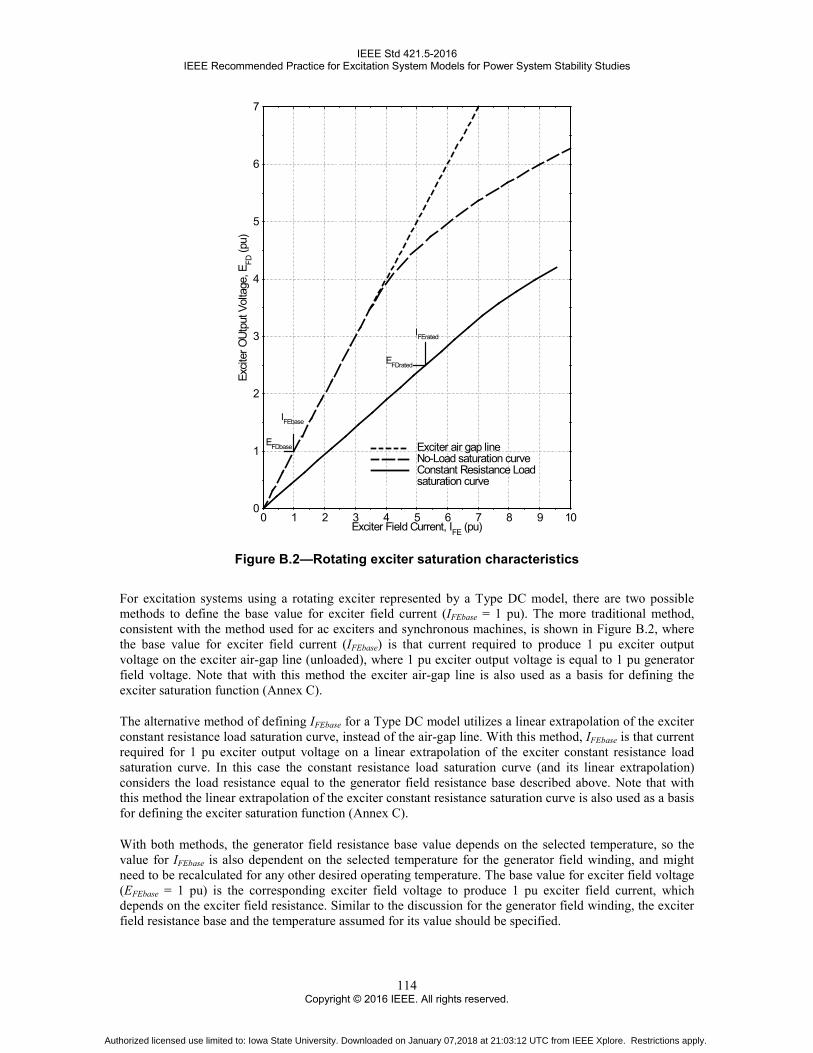
IEEE Std 421.5-2016 IEEE Recommended Practice for Excitation System Models for Power System Stability Studies
0
1
2
3
4
5
6
7
0 1 2 3 4 5 6 7 8 9 10
Exciter air gap lineNo-Load saturation curveConstant Resistance Loadsaturation curve
IFErated
EFDrated
IFEbase
EFDbase
Exciter Field Current, IFE (pu)
Excit
er O
Utpu
t Vol
tage
, EFD
(pu)
Figure B.2—Rotating exciter saturation characteristics
For excitation systems using a rotating exciter represented by a Type DC model, there are two possible methods to define the base value for exciter field current (IFEbase = 1 pu). The more traditional method, consistent with the method used for ac exciters and synchronous machines, is shown in Figure B.2, where the base value for exciter field current (IFEbase) is that current required to produce 1 pu exciter output voltage on the exciter air-gap line (unloaded), where 1 pu exciter output voltage is equal to 1 pu generator field voltage. Note that with this method the exciter air-gap line is also used as a basis for defining the exciter saturation function (Annex C).
The alternative method of defining IFEbase for a Type DC model utilizes a linear extrapolation of the exciter constant resistance load saturation curve, instead of the air-gap line. With this method, IFEbase is that current required for 1 pu exciter output voltage on a linear extrapolation of the exciter constant resistance load saturation curve. In this case the constant resistance load saturation curve (and its linear extrapolation) considers the load resistance equal to the generator field resistance base described above. Note that with this method the linear extrapolation of the exciter constant resistance saturation curve is also used as a basis for defining the exciter saturation function (Annex C).
With both methods, the generator field resistance base value depends on the selected temperature, so the value for IFEbase is also dependent on the selected temperature for the generator field winding, and might need to be recalculated for any other desired operating temperature. The base value for exciter field voltage (EFEbase = 1 pu) is the corresponding exciter field voltage to produce 1 pu exciter field current, which depends on the exciter field resistance. Similar to the discussion for the generator field winding, the exciter field resistance base and the temperature assumed for its value should be specified.
114 Copyright © 2016 IEEE. All rights reserved.
Authorized licensed use limited to: Iowa State University. Downloaded on January 07,2018 at 21:03:12 UTC from IEEE Xplore. Restrictions apply.

IEEE Std 421.5-2016 IEEE Recommended Practice for Excitation System Models for Power System Stability Studies
Annex C
(normative)
Saturation function and loading effects
C.1 General
Information in this annex relates to both the saturation characteristics of the generator (synchronous machine) and the saturation characteristics of a rotating exciter used as part of an excitation control system. The saturation function, generally designated as S(E) or as SE(E) for rotating exciters, is used to determine the amount of field current beyond the air-gap line that is needed to provide a specified generator or exciter output voltage.
C.2 Generator saturation
Although the generator saturation function is not included as part of the excitation system model, it is considered here to point out both the similarities and differences in how the generator and rotating exciter saturation functions are defined in models and expressed as input data to power system simulation programs. Refer to IEEE Std 1110 and IEEE Std 115 for further details of generator modeling and testing, respectively.
Figure C.1 shows the values on the generator open-circuit saturation curve and air-gap line used to calculate saturation factors due to magnetic saturation of the generator. At a given generator terminal voltage (E), the difference between the field current on the open-circuit saturation curve and the field current on the air-gap line is used to determine the saturation function S(E). The input data protocol for most synchronous machine models requires saturation factors to be provided at two values of terminal voltage, 1.0 pu and 1.2 pu, with saturation factors defined using Equation (C.1) and the values in Figure C.1 (Anderson and Fouad [B1]):
( )
( )2
23
0
01
pu 2.1
pu 0.1
FD
FDFD
FD
FDFD
III
S
III
S
−=
−=
(C.1)
These saturation factors S(1.0) and S(1.2) are non-dimensional and thus can be calculated with the field currents measured in physical units, per unit, or even from direct measurement (in mm or inches, for instance) from a plot of the generator open-circuit saturation curve. A mathematical expression of the saturation function S(E) for the generator is typically derived by applying an appropriate curve fit using these two saturation factors. Different mathematical functions have been used to represent generator saturation, including quadratic, exponential, and geometric functions.
115 Copyright © 2016 IEEE. All rights reserved.
Authorized licensed use limited to: Iowa State University. Downloaded on January 07,2018 at 21:03:12 UTC from IEEE Xplore. Restrictions apply.

IEEE Std 421.5-2016 IEEE Recommended Practice for Excitation System Models for Power System Stability Studies
00
Air-Gap LineOpen Circuit Saturation Curve
IFD0
Generator Field Current
IFD3IFD2IFD1
1.2 x Rated Terminal Voltage
1.0 x Rated Terminal Voltage
Gen
erat
or T
erm
inal
Vol
tage
Figure C.1—Generator open-circuit saturation characteristics
C.3 Rotating exciter saturation
Depending upon the excitation system model, the function SE(E) for representing rotating exciter saturation utilizes either the exciter no-load saturation curve or the exciter constant resistance load saturation curve. Figure C.2 illustrates curves and values used in the calculation of the appropriate saturation factor for various types of rotating exciters. At a given exciter output voltage EX, current A is the exciter field current on the exciter constant resistance load saturation curve, current B is the exciter field current on the air-gap line, and current C is the exciter field current on the exciter no-load saturation curve.
For all Type AC models (except the superseded type AC5A model), the exciter no-load saturation curve is used in defining the saturation factors for the saturation function SE(VE) (see Figure 8). Although saturation in the Type AC models is a function of alternator output voltage VE, the calculation of the saturation function can instead utilize the no-load saturation curve of the exciter output voltage EFD, since the per-unit values of VE and EFD are the same for the unloaded exciter. If the exciter output voltage in Figure C.2 is expressed in pu, the no-load saturation curve and air-gap line are the same for both EFD and VE. Thus the Type AC exciter saturation factors used to determine SE(VE) can instead be calculated as SE(EFD). Using the exciter no-load saturation curve for either VE or EFD, SE(VE) is defined in Equation (C.2) using the values shown in Figure C.2:
( ) ( )B
BCIESVS FDFDEEE−
=== 0, (C.2)
116 Copyright © 2016 IEEE. All rights reserved.
Authorized licensed use limited to: Iowa State University. Downloaded on January 07,2018 at 21:03:12 UTC from IEEE Xplore. Restrictions apply.

IEEE Std 421.5-2016 IEEE Recommended Practice for Excitation System Models for Power System Stability Studies
B*
Exciter Field Current
Excit
er O
utpu
t Vol
tage Ex
B C A
constant resistanceloadsaturation
no-load saturation
air gap line
Figure C.2—Exciter saturation characteristics
The no-load saturation curve and saturation function SE(VE) for alternator-rectifier exciters is used to model only the effects of magnetic saturation, because exciter regulation effects are separately represented by inclusion of a demagnetizing factor KD and a rectifier regulation function FEX in the model (Annex D).
For all Type DC rotating exciter models (and also the superseded type AC5A model), the constant-resistance load saturation curve is used in defining the saturation factors for the saturation function SE(EFD) (see Figure 3). In these cases, SE(EFD) is defined by Equation (C.3) using the values shown in Figure C.2:
BBAES FDE
−=)( (C.3)
For all Type DC rotating exciter models the specific values used for B in Equation (C.3) depend upon the method in which the base value of exciter field current (IFEbase) is defined for an exciter represented in a Type DC model (Annex B). If IFEbase is defined based on the more traditional use of the exciter air-gap line, then the values of B in Equation (C.3) are from the exciter air-gap line. If IFEbase is defined based on the alternative use of the linear extrapolation of the exciter constant resistance load saturation curve, then the values of B in Equation (C.3) are from the linear extrapolation of the exciter constant resistance load saturation curve, shown as the point B* in Figure C.2.
For Type DC models the effects of both magnetic saturation and load regulation are combined into one saturation function, and thus the exciter constant resistance load saturation curve is used to determine and represent these combined effects.
117 Copyright © 2016 IEEE. All rights reserved.
Authorized licensed use limited to: Iowa State University. Downloaded on January 07,2018 at 21:03:12 UTC from IEEE Xplore. Restrictions apply.

IEEE Std 421.5-2016 IEEE Recommended Practice for Excitation System Models for Power System Stability Studies
Equation (C.2) and Equation (C.3) define the saturation factors as ratios of exciter field current and, thus, these saturation factors are non-dimensional and can be calculated from Figure C.2 with the horizontal axis measured in physical quantities, per unit, or direct measurement.
Note that when the exciter field resistance is significantly different from the exciter field resistance base used to determine EFEbase, an adjusted value of the saturation function may be used as described in Annex A of the 1983 IEEE Committee Report [B23].
Different computer programs have represented the exciter saturation characteristic with different mathematical expressions. In general, the saturation function can be defined adequately by two points. To be consistent, the suggested procedure specifies two exciter output voltages E1 and E2 at which to specify the saturation factors SE(E1) and SE(E2) for the exciter saturation function. These data points may then be used as input parameters for the excitation system model. The mathematical function to represent the saturation function as a curve fit of the specified points is not defined here, but rather considered to be a part of the particular computer program used.
In general, the saturation factors of the rotating exciter would be specified as shown in Table C.1:
Table C.1—Parameters for definition of rotating exciter saturation Rotating exciter model type Exciter voltages Saturation factors
Type DC rotating exciter model and superseded AC5A model (Figure 3)
EFD1, EFD2 SE(EFD1), SE(EFD2) (value calculated as shown in Equation C.3)
Type AC rotating exciter model (Figure 8)
VE1, VE2 (= EFD1, EFD2 in pu on no-load curve)
SE(VE1), SE(VE2) or SE(EFD1), SE(EFD2) (values calculated as shown in Equation C.2)
Saturation effects are most significant at higher exciter output voltages. For dc commutator rotating exciters, since the highest exciter output voltage occurs during the maximum positive forcing condition, the exciter output voltages EFD1 and EFD2, used to define SE(EFD1) and SE(EFD2), should be at or near the exciter ceiling voltage and at a lower value, usually near 75% of the exciter ceiling voltage. Similarly, for the alternator-rectifier exciters, the exciter voltages VE1 and VE2 (or EFD1 and EFD2), used to define SE(VE1) and SE(VE1), should be at or near the exciter no-load ceiling voltage and at a lower value, usually near 75% of the exciter no-load ceiling voltage.
In some cases, such as a self-excited dc exciter, the ceiling voltage may not be precisely known because it depends on KE. In such cases, the saturation factors are obtained at a specified value of exciter voltage at or near its expected maximum value. The second saturation point is then specified at a lower value, usually around 75% of the first selected value.
118 Copyright © 2016 IEEE. All rights reserved.
Authorized licensed use limited to: Iowa State University. Downloaded on January 07,2018 at 21:03:12 UTC from IEEE Xplore. Restrictions apply.

IEEE Std 421.5-2016 IEEE Recommended Practice for Excitation System Models for Power System Stability Studies
Annex D
(normative)
Rectifier regulation
All ac sources that supply rectifier circuits in excitation systems have an internal impedance that is predominantly inductive. The effect of this impedance extends the process of commutation and causes a non-linear decrease in rectifier average output voltage as the rectifier load current increases. The three-phase full-wave bridge rectifier circuits commonly employed have three distinct modes of operation. The rectifier load current determines the particular equations characterizing each of these three modes. Figure D.1 shows the rectifier regulation characteristics determined by the equations shown in Figure D.2. For small values of KC, only mode 1 operation need be modeled, as is done in the Type ST1C model shown in 8.3.
The quantities EFD, IFD, VE, and KC are all expressed in per unit on the synchronous machine field base. For computer simulation purposes, the curve of Figure D.1 is defined by three segments as shown by the equations in Figure D.2.
Note that IN should not be greater than 1. However, if IN is greater than 1 for any reason, the model should set FEX equal to 0. If IFD is less than zero or IN is less than zero, the condition should be flagged and the considerations of Annex G would then apply. Further information may be found in ANSI C34.2-1968 [B3], Witzke, Kresser, and Dillard [B53] and Krause, Wasynczuk, and Sudhoff [B32].
The rectifier regulation can have a significant impact on the ceiling generator field voltage EFD. In the Type ST1C model shown in 8.3, the ceiling value for the generator field voltage EFD is determined by the output limit of the model as given in Equation (D.1):
( ) ( ) FDCSTCRTceilingFD IKVVE ×−×= 1max (D.1)
For excitation system models using the rectifier model shown in Figure D.2, such as the Type ST4C model shown in 8.9, the ceiling value for the generator field voltage EFD is determined by the output limit on the AVR control path and also the effect of the rectifier model on its output signal VB. In the example of the Type ST4C model, the ceiling can be calculated as given in Equation (D.2):
( ) ( )NEXEMBMceilingFD IFVVVVE ××=×= maxmax (D.2)
For comparison with the Type ST1C model, it is assumed that VE = KP × VT and the rectifier model is also operating on mode 1. Therefore Equation (D.2) can be expressed as shown in Equation (D.3):
( ) ( )
( ) FDCSTCMP
TPM
T
FDCSTCTPMceilingFD
IKVKVKV
VIKVKVE
××
−××=
=
−×××=
4max
max
4max
3
311
(D.3)
119 Copyright © 2016 IEEE. All rights reserved.
Authorized licensed use limited to: Iowa State University. Downloaded on January 07,2018 at 21:03:12 UTC from IEEE Xplore. Restrictions apply.

IEEE Std 421.5-2016 IEEE Recommended Practice for Excitation System Models for Power System Stability Studies
To represent the same ceiling value for the generator field voltage EFD in the Type ST1C and Type ST4C models, the following relationships should exist between the parameters in these models, based on a comparison of Equation (D.1) and Equation (D.3):
( ) ( ) CSTCMP
CSTC
PMR
KVKK
KVV
4max
1
maxmax
3×
=
×= (D.4)
0
0.2
0.4
0.6
0.8
1.0
1.2
0 0.2 0.4 0.6 0.8 1.0 1.2
EFD
VE
KC IFD
VEIN=
slope = 3
slope = 3
1
MODE 3
MODE 2
MODE 1
Figure D.1—Rectifier regulation characteristic
FEX
IN
ΠVE
IN=KCIFD
VEIFD
VB
IF IN ≤ 0.433 FEX = 1 − 0.577 IN
FEX = 0.75 −(IN)2
FEX = 1.732 (1 − IN)
FEX = 0
IF 0.433
IF 1
IF 0.75
IN ≤ 0.75
IN
IN ≤ 1
<
<
<
Figure D.2—Rectifier regulation equations (function FEX)
The voltage VE in Figure D.2 represents the ac voltage at the input of the rectifier bridge. In general, this ac voltage is the secondary voltage of an excitation transformer or is provided by a pilot exciter. Figure D.3 presents the overall model to represent the power source for the excitation system, combining the rectifier regulation model shown in Figure D.2 with the representation of an excitation transformer (input “A” in the logic switch SW1) or the representation of an ac power source independent from the generator terminal conditions, such as a pilot exciter (position “B” of the logic switch SW1).
120 Copyright © 2016 IEEE. All rights reserved.
Authorized licensed use limited to: Iowa State University. Downloaded on January 07,2018 at 21:03:12 UTC from IEEE Xplore. Restrictions apply.

IEEE Std 421.5-2016 IEEE Recommended Practice for Excitation System Models for Power System Stability Studies
FEX=f(IN)
FEX
IN
Π
KP=KP θP–
–IT
VT–
IFD
VB
VBmax
VE
IN=KCIFD
VE
SW1(a)
KP
yy=|KP∙VT+j(KI+KP∙XL)∙IT|
– – ––A
B
footnotes:
SW1 is a user-selection option. Position A corresponds to a power source derived from generator terminal voltage, such as an excitation transformer. Position B corresponds to a power source independent of generator terminal conditions.
(a)
Figure D.3—Representation of the power source
The variable y represents the ac voltage at the secondary of the excitation transformer and is calculated based on the generator terminal voltage VT. Additionally, it is possible to represent the effect of compound windings in the excitation transformer (IEEE Committee Report, 1983 [B23]), so the ac voltage at the secondary of the excitation transformer has a component proportional to the generator terminal current IT.
When representing a conventional (potential) excitation transformer, the parameter KP should be greater than zero, while the parameters associated with the compound windings (KI and XL) should be set equal to zero. In this case, the phase angle for KP (parameter θP) becomes irrelevant for the calculation of the magnitude of the parameter y, and therefore θP is commonly set to zero.
When representing a compound excitation transformer, the parameters KI and/or XL would have nonzero values. In such case, the proper phasor calculation shown in Figure D.3 should be applied and therefore the phase relationships become fundamental, so θP would have to be set accordingly.
It should also be noted that the current IN is a normalized current, with a value ranging between 0 and 1, as shown in Figure D.2. Thus, the calculation of the parameter KC, shown in Equation (D.4), has to take into consideration the value for the magnitude of the parameter KP.
121 Copyright © 2016 IEEE. All rights reserved.
Authorized licensed use limited to: Iowa State University. Downloaded on January 07,2018 at 21:03:12 UTC from IEEE Xplore. Restrictions apply.

IEEE Std 421.5-2016 IEEE Recommended Practice for Excitation System Models for Power System Stability Studies
Annex E
(normative)
Block diagram representations
E.1 General This annex describes the most common blocks used in the block diagrams presented in this recommended practice. Several of these blocks are relatively straightforward, but there are possible different implementations for some of these blocks, particularly when limits are applied. This annex serves as the reference for the intended implementation of the individual blocks in the block diagrams of the models presented in this recommended practice.
Two distinct types of limiters, windup and non-windup, are represented in the models. Implementation of the different types of limiters for several model blocks is described in the following clauses.
E.2 Simple integrator The functions of these two types of limits, as applied to simple integrator blocks, are illustrated in Figure E.1 and Figure E.2.
Note the difference in block diagram notation of the two types of limiters. With the non-windup limiter (see Figure E.2), starting from a limited condition with y = A or y = B, the output of the block y begins to change in value as soon as the input to the block changes sign. This is not the case with the windup limiter (see Figure E.2), where the integrator output y should first integrate back to the limiter setting before the output x can come off the limit.
dy/dt = [ 1 / T ] u
→ x = B
OTHERWISE
x = A
x = y
IF y ≥ B
IF y ≤ A
B
A
1
sT
u y x
→
→ Figure E.1—Integrator with windup limiter
dy/dt = [ 1 / T ] u
→ x = B
OTHERWISE
x = A
x = y
IF y ≥ B
IF y ≤ A
B
A
1
sT
u x
→
→
dy/dt = 0
dy/dt = 0
Figure E.2—Integrator with non-windup limiter
122 Copyright © 2016 IEEE. All rights reserved.
Authorized licensed use limited to: Iowa State University. Downloaded on January 07,2018 at 21:03:12 UTC from IEEE Xplore. Restrictions apply.

IEEE Std 421.5-2016 IEEE Recommended Practice for Excitation System Models for Power System Stability Studies
E.3 Simple time constant
Figure E.3 and Figure E.4 show the representation and implementation of single time constant blocks with windup and non-windup limiters.
It should be noted that in the case of a windup limit, the variable y is not limited. Therefore when the output variable x hits a limit, it cannot come off the limit until y comes within the limits.
In the case of the non-windup limit, to be at a limit x = y = A or x = y = B, implies input u < A or u > B, respectively. With this limiter, the output comes off the limit as soon as the input u re-enters the range within the limits defined by A < u < B.
dy/dt = [ u – y ] / T
→ x = B
OTHERWISE
x = A
x = y
IF y ≥ B
IF y ≤ A
B
A
u y x
→
→
1
1+sT
Figure E.3—Simple time constant with windup limiter
B
A
u x1
1+sT
–Σ
+
u
B
A
1
sT
x
dy/dt = [ u – y ] / T
→ x = B
OTHERWISE
x = A
x = y
IF y ≥ B
IF y ≤ A →
→
dy/dt = 0
dy/dt = 0
(a) Block diagram (b) Implementation
Figure E.4—Simple time constant with non-windup limiter
123 Copyright © 2016 IEEE. All rights reserved.
Authorized licensed use limited to: Iowa State University. Downloaded on January 07,2018 at 21:03:12 UTC from IEEE Xplore. Restrictions apply.

IEEE Std 421.5-2016 IEEE Recommended Practice for Excitation System Models for Power System Stability Studies
E.4 Lead-lag block
A block diagram representation and equations for a windup limiter applied to a lag-lead block are provided in Figure E.5.
u
OTHERWISE
→
→
x = A
x = y
IF y ≥ B
IF y ≤ A
→ x = B
IF (T1 = T2) or (T2 = 0) → x = u (block by-passed)
1+sT1
1+sT2
B
A
xy
Figure E.5—Lead-lag block with windup limiter
Figure E.6 shows the block diagram representation for a non-windup limiter applied to a lag-lead block, along with equations and a diagram showing how it is realized. Other models of non-windup limiting of a lag-lead block are possible, but this one is considered to most accurately represent the behavior of most digital implementations of lag-lead functions.
u 1+sT1
1+sT2
B
A
x
(T1 > 0) and (T2 > 0)
OTHERWISE
→
→
x = A
x = y
IF y ≥ B
IF y ≤ A
→ x = B
ΣT1
T2
–
+
B
A
Σ1
sT1
−1T2
T1
+
+
u xy
(a) Block diagram (b) Implementation
Figure E.6—Lead-lag block with non-windup limiter
124 Copyright © 2016 IEEE. All rights reserved.
Authorized licensed use limited to: Iowa State University. Downloaded on January 07,2018 at 21:03:12 UTC from IEEE Xplore. Restrictions apply.

IEEE Std 421.5-2016 IEEE Recommended Practice for Excitation System Models for Power System Stability Studies
E.5 Proportional-integral (PI) block
The use of proportional-integral regulator blocks in the models ST4C, ST6C, ST8C, AC7C, and AC11C requires the definition of the implementation of the non-windup limit in the PI blocks in these computer models, as defined in Figure E.7.
B
A
KP+KI
s
u x
OTHERWISE
→
→
x = A dz/dt = 0
x = y dz/dt = KI u
IF y ≥ B
IF y ≤ A
→ x = B dz/dt = 0
+
B
A
+
u xyΣKP
1
s
zKI
(a) Block diagram (b) Implementation
Figure E.7—Proportional-integral block with non-windup limiter
The ST7C model implements a non-windup proportional-integral function as represented in Figure E.8. If a non-linearity is acting (that means a saturation is reached or a low value (LV) or high value (HV) comparator imposes another signal “w” calculated by another function, for example an over or underexcitation limiter as the output signal), then the low-pass filter output follows the PI output signal, insuring a non-windup behavior of the PI function integrator. The input signal of the low-pass filter of time constant Ti is the PI output signal, after application of all non-linearity treatments.
B
A
KP+KI
s
u x
ΣKP+
B
A
+
u xyLVor HV
w
1
1+sTITI =
KP
KI (a) Block diagram (b) Implementation
Figure E.8—Alternative implementation of non-windup proportional-integral block
The PI controller in Figure E.8 is implemented according to the following principle:
ΣKP+
+
u x
1
1+sTI
non-linearities
125 Copyright © 2016 IEEE. All rights reserved.
Authorized licensed use limited to: Iowa State University. Downloaded on January 07,2018 at 21:03:12 UTC from IEEE Xplore. Restrictions apply.

IEEE Std 421.5-2016 IEEE Recommended Practice for Excitation System Models for Power System Stability Studies
The error signal u is the input signal of the function. The signal x is its output. The non-linearities can be a saturation of the output signal, or a HV gate or LV gate with any other signal. If no non-linearities are acting, the transfer function can be calculated as follows:
usT
sTKxuKx
sTx
sTuKx
I
IPP
IIP
+=⇔=
+
−⇔+
+=1
111
11 (E.1)
The transfer function of this diagram is:
I
IP sT
sTK
ux +=
1 (E.2)
Then this diagram represents a PI controller. This representation provides a non-windup behavior of the integrator.
E.6 Proportional-integral-derivative (PID) block
Several models utilize proportional-integral-derivative (PID) regulators with non-windup limits. They require some definition of the non-windup modeling for implementation of the computer models.
Often the parallel form of a PID controller with the transfer function
( )D
DIP sT
sKs
KKsK
+++=
1 (E.3)
is realized by the sum of the three terms: the proportional term with the proportional gain KP, the integral term with the integral gain KI, and the derivative term with the derivative gain KD and the lag time constant TD. To avoid windup effects of the integral term, a non-windup modeling according to Figure E.9 is required similar to the non-windup scheme of a PI controller (see Figure E.7). If the sum y hits the limits, the integration is stopped. Other models of non-windup limiting of a PID controller are possible, but this one is considered to represent an easy-to-implement principle in digital control and simulation.
126 Copyright © 2016 IEEE. All rights reserved.
Authorized licensed use limited to: Iowa State University. Downloaded on January 07,2018 at 21:03:12 UTC from IEEE Xplore. Restrictions apply.

IEEE Std 421.5-2016 IEEE Recommended Practice for Excitation System Models for Power System Stability Studies
B
A
u xKP+
KI
s+
sKD
1+sTD
OTHERWISE
→
→
x = A dz/dt = 0
x = y dz/dt = KI u
IF y ≥ B
IF y ≤ A
→ x = B dz/dt = 0
+
B
A
+
u xyΣKP
1
s
zKI
KDs
1+sTD
(a) Block diagram (b) Implementation
Figure E.9—Proportional-integral-derivative block with non-windup limit
An alternative implementation of the PID regulator with non-windup limits is applied in the Type AC11C model (7.20), which is represented as shown in Figure E.10.
B
A
u xKP+
KP
sTI)( 1+
sKBTB
KB+sTB)(
OTHERWISE
→
→
x = A dz/dt = 0
x = y dz/dt = (KP/TI) u
IF y ≥ B
IF y ≤ A
→ x = B dz/dt = 0
+
uKP
1
s
zKP
TI
B
A
+
xyΣΣ
+
Σ KB
1
sTB
++
–
(a) Block diagram (b) Implementation
Figure E.10—Alternative proportional-integral-derivative block with non-windup limit
E.7 Washout block
A block diagram representation for a washout (high-pass filter) is provided in Figure E.11. As applied in the PSS2C stabilizer, some washouts may not be used. In this case, the block should be bypassed (its output set equal to its input). Bypassing the block is denoted by setting its time constant, TW, equal to zero.
sTW
1+sTW
u x
IF (TW = 0) → x = u (block by-passed) Figure E.11—Washout block
127 Copyright © 2016 IEEE. All rights reserved.
Authorized licensed use limited to: Iowa State University. Downloaded on January 07,2018 at 21:03:12 UTC from IEEE Xplore. Restrictions apply.

IEEE Std 421.5-2016 IEEE Recommended Practice for Excitation System Models for Power System Stability Studies
E.8 Filtered derivative block
In Figure E.12 the block diagram (a) and the implementation (b) of a derivative element are illustrated. The equations of Figure E.11 show how the implementation is modeled. The derivative block with a limit is used in the AC9C model, as part of its regulator structure. The limiter is needed to allow the proper function of other excitation elements such as limiters or to model analog or numerical limited systems. To disable the limits, A and B can be set to infinite.
It should be noted that there is no difference between a windup or a non-windup limit applied to the filtered derivative block. Therefore, the same implementation can be used to either type of block diagram shown in Figure E.12(a).
u xsKD
1+sTD
B
A
u xsKD
1+sTD
B
A OTHERWISE
→
→
x = A
x = y
IF y ≥ B
IF y ≤ A
→ x = B
+
B
Au
xy
y1
KD
TD
Σ1
sTDu1–
u1 = u − y1
dy1/dt = [ 1 / TD ] u1
y = [ KD / TD ] u1
(a) Block diagram (b) Implementation
Figure E.12—Filtered derivative block with limiter
E.9 Logical switch block
Figure E.13 presents the graphical representation of a logical switch. In its most basic form, the parameter SW1 represents a user-selection (constant parameter) with two possible values. This recommended practice is not defining how these possible values should be defined, but SW1 could be a numerical value such as 0 or 1, or SW1 could be a character value such as “A” or “B.” In this basic form, the switch block represents two possible values for the output signal y, and the definition of which input signal (uA or uB) to use is fixed, determined by the selected value for the parameter SW1.
IF SW1 = (option B) → y = uB
OTHERWISE → y = uA
SW1
uA
yuB
A
B
Figure E.13—Logical switch block
128 Copyright © 2016 IEEE. All rights reserved.
Authorized licensed use limited to: Iowa State University. Downloaded on January 07,2018 at 21:03:12 UTC from IEEE Xplore. Restrictions apply.

IEEE Std 421.5-2016 IEEE Recommended Practice for Excitation System Models for Power System Stability Studies
In a more general form, SW1 could be a signal calculated as a function of other signals in the model and, therefore, the definition of which input signal to use could change during a simulation, as SW1 could change its value.
Notes have been added to the block diagrams that use this switch block or any other form of a logical block, so the logic described on these specific notes should supersede the definition shown in Figure E.13, in case of any discrepancies.
129 Copyright © 2016 IEEE. All rights reserved.
Authorized licensed use limited to: Iowa State University. Downloaded on January 07,2018 at 21:03:12 UTC from IEEE Xplore. Restrictions apply.

IEEE Std 421.5-2016 IEEE Recommended Practice for Excitation System Models for Power System Stability Studies
Annex F
(informative)
Avoiding computational problems by eliminating fast-feedback loops
F.1 General
The models represented in the body of this document are reduced order models, which do not contain all of the feedback loops of the physical system.
The models are valid for oscillation frequencies up to about 3 Hz and simulation software integration time steps of typically ¼ of a cycle. This annex discusses the elimination of fast-feedback loops. The direct simulation of these loops using such time steps could result in computational problems. Therefore such computation problems have been avoided in the models by simulating the loops indirectly as limiters.
F.2 Type AC3C excitation system model
F.2.1 Minimum field voltage limiter loop
The recommended model for the Type AC3C system is shown in Figure 11. The lower limiter on the exciter voltage VE is not a physical limit. The physical system contains a fast-feedback loop that limits the field voltage, as shown in Figure F.1.
EFEΠ
VF
+–
VA
KA
1+sTA
VAmax
VAmin
Σ HV gate
KLV Σ
+–
EFD
VLV
Figure F.1—Minimum field voltage limiter loop for the
Type AC3C alternator-rectifier exciter
The output of the field limiter loop is normally the lower of the two parameters entering the high value (HV) gate. As such, it has no effect on the excitation system output. As the field voltage drops, the output of the loop increases. As the field voltage decreases to approximately VLV, the output of the loop becomes the greater of the two parameters entering the gate and an error signal is produced to boost the field voltage.
The field voltage limiter loop is a fast loop with a natural frequency of oscillation greater than 4.0 Hz. Direct simulation of this loop in a stability study would require time steps smaller than those normally used in stability studies. The recommended model in Figure 11 simulates the loop as a lower limiter on the exciter voltage.
130 Copyright © 2016 IEEE. All rights reserved.
Authorized licensed use limited to: Iowa State University. Downloaded on January 07,2018 at 21:03:12 UTC from IEEE Xplore. Restrictions apply.

IEEE Std 421.5-2016 IEEE Recommended Practice for Excitation System Models for Power System Stability Studies
F.2.2 Derivation of minimum exciter voltage
The equations representing the steady-state position of the exciter voltage can be obtained from Figure 11 and Figure F.1 as follows:
( )( )FDLVFDLVRAFEFE EVEKKKEV −×××== (F.1)
( )[ ] FDDEEEEFE IKVVSKV ×++= (F.2)
( ) ENEXFD VIFE ×= (F.3)
Solving Equation (F.1) through Equation (F.3) for EFD, then substituting EFDmin for EFD,
2
1
GIKVGE FDDLV
FDmin×−×
= (F.4)
where
FDminLVRA EKKKG ×××=1 (F.5)
( )( )NEX
EEEIF
VSKGG ++= 12 (F.6)
Since G1 is very large (70 to 1000), EFDmin can be approximated as:
LVFDmin VE ≅ (F.7)
The minimum steady-state limit for the exciter voltage can be obtained by substituting Equation (F.7) into Equation (F.3).
( )NEX
LVEmin IF
FV ≅ (F.8)
F.2.3 Maximum field current limiter loop
The recommended model for the AC3A system is shown in Figure 11. The upper limiter on the exciter voltage VE, is not a physical limit. The physical system contains a fast-feedback loop that limits the exciter field current. This loop is shown in Figure F.2.
The output of the field current limiter loop is normally zero. As the field current VFE increases, the output of this loop decreases. When the field current multiplied by KFA exceeds ETX, the output of the loop comes off its limit and an error signal to decrease the excitation is produced, thus limiting the field current.
131 Copyright © 2016 IEEE. All rights reserved.
Authorized licensed use limited to: Iowa State University. Downloaded on January 07,2018 at 21:03:12 UTC from IEEE Xplore. Restrictions apply.

IEEE Std 421.5-2016 IEEE Recommended Practice for Excitation System Models for Power System Stability Studies
The field current limiter loop is a fast loop with a natural frequency of oscillation greater than 4.0 Hz. Direct simulation of this loop in a stability study would require time steps smaller than those normally used in stability studies. The recommended model in Figure 11 simulates the loop as an upper limiter on the exciter voltage.
EFEΠ
VF
+–
VA
KA
1+sTA
VAmax
VAmin
Σ
+–
ETX
+
VLKL1 Σ
0
Σ
VFEKFA
1+sTFA
+–
Figure F.2—Maximum field current limiter loop for the Type AC3C
alternator-rectifier exciter with alternator field current limiter
F.2.4 Derivation of maximum exciter voltage
The equations representing the steady-state position of the exciter voltage can be obtained from Figure 11 and Figure F.2 as follows:
( )FEFATXLL VKEKV ×−×= 1 (F.9)
( )( )FerrSLFDRAFEFE VVVVEKKEV −++××== (F.10)
( )[ ] FDDEEEEFE IKVVSKV ×++= (F.11)
( ) ENEXFD VIFE ×= (F.12)
CREFerr VVV −= (F.13)
The exciter stabilizer output VF is zero in the steady-state. The output decays to zero, however, with a relatively long time constant TF, which is approximately 1.0 seconds. The other time constants in the system vary from 0.01 to 0.02 seconds with the exception of TE, which is approximately 1.0 seconds. Although TE is large, the effective time constant is quite small due to the large gains KA and KR.
By combining these equations, setting VF equal to zero, and substituting VFEmax for VFE,
( )11
11 1 LFA
errSTXLFEmax KKGGVVEKV
××+++×= (F.14)
132 Copyright © 2016 IEEE. All rights reserved.
Authorized licensed use limited to: Iowa State University. Downloaded on January 07,2018 at 21:03:12 UTC from IEEE Xplore. Restrictions apply.

IEEE Std 421.5-2016 IEEE Recommended Practice for Excitation System Models for Power System Stability Studies
where
( ) EmaxNEXRA VIFKKG ×××=1 (F.15)
The typical values of the parameters when the field voltage is near ceiling are given below:
TXL EK ×1 = 0.93
VS = 0.0 to 0.10 Verr = 0.0 to 1.0 G1 = 1000
11 LFA KKG ×× = 56
Assuming the above typical values, Equation (F.14) can be simplified:
1
1
LFA
errSTXLFEmax KK
VVEKV×
++×= (F.16)
Solving Equation (F.11) for VE, then substituting VEmax for VE:
( )EEE
FDDFEmaxEmax VSK
IKVV+
×−= (F.17)
F.3 Other Type AC excitation system models
F.3.1 Maximum field current limiter loop (fast OEL)
As an example, consider the recommended model for the Type AC2C system shown in Figure 10. Rather than the upper limiter on the exciter voltage VE being a physical limit, the actual physical system contains a fast-feedback loop that limits the exciter field current as shown in Figure F.3.
VA
EFEmax
EFEmin
VFE
EFEΣ
1
sTE VE–+
LV gate
KH
Σ
–+
VH
KB
KL ΣVL
–+VLR
Figure F.3—Maximum field current limiter loop for the Type AC2C
high initial response alternator-rectifier excitation system with non-controlled rectifiers and feedback from exciter field current
133 Copyright © 2016 IEEE. All rights reserved.
Authorized licensed use limited to: Iowa State University. Downloaded on January 07,2018 at 21:03:12 UTC from IEEE Xplore. Restrictions apply.

IEEE Std 421.5-2016 IEEE Recommended Practice for Excitation System Models for Power System Stability Studies
The output of the fast field current limiter loop VL is normally the higher of the two parameters entering the LV gate. As such, it has no effect on the excitation system output. As the exciter field current VFE increases, the output of the loop decreases. As the field current increases to approximately VLR, the output of the loop becomes the lower of the two parameters entering the gate and an error signal is produced to decrease the field current.
The effective time constant for the field current limiter loop is approximately 1.0 ms and direct simulation of this loop would require time steps smaller than those normally used in stability studies. The recommended model in Figure 10 simulates the loop as an upper limit on the exciter voltage.
F.3.2 Derivation of maximum exciter voltage
The equations representing the steady-state position of the exciter voltage can be obtained from Figure F.2 and Figure F.3, as follows:
( )FELRBLFEFE VVKKEV −××== (F.18)
( )[ ] FDDEEEEFE IKVVSKV ×++= (F.19)
Solving Equation (F.18) for VFE then substituting VFEmax for VFE,
LRLRBL
BLFE VV
KKKKV ≅×+
×=
1max (F.20)
Solving Equation (F.19) for VE, then substituting VFEmax and VEmax for VFE and VE, respectively,
( )EEE
FDDFEE VSK
IKVV+
×−= max
max (F.21)
If there is no fast OEL then set VFEmax to a large number so that the limit is disabled.
134 Copyright © 2016 IEEE. All rights reserved.
Authorized licensed use limited to: Iowa State University. Downloaded on January 07,2018 at 21:03:12 UTC from IEEE Xplore. Restrictions apply.

IEEE Std 421.5-2016 IEEE Recommended Practice for Excitation System Models for Power System Stability Studies
Annex G
(normative)
Paths for flow of induced synchronous machine negative field current
G.1 General
AC and ST Type exciters cannot deliver negative field current because they have rectifiers at their output. Under some conditions a negative current may be induced in the field of the synchronous machine (de Mello, Leuzinger, and Mills [B40]). If this current is not allowed to flow, a dangerously high voltage may result. In some cases, damper windings or solid iron rotor effects may limit the maximum voltage experienced by the field winding and rectifiers under such conditions, but in other cases circuitry is provided to allow negative field currents to flow, bypassing the exciter itself. These take the form of either “crowbar” circuits (field shorting) or non-linear resistors (varistors), as shown in Figure G.1.
In the case of the crowbar, a linear or non-linear resistor is inserted across the field of the synchronous machine by thyristors that are triggered on the overvoltage produced when the field current attempts to reverse and is blocked by the rectifiers on the output of the exciter.
Varistors are non-linear resistors that may be permanently connected across the field of the synchronous machine. During normal conditions, the resistance of these devices is very high and small currents flows through them. The varistor current increases very rapidly as the voltage across it is increased beyond a threshold level and thus limits the voltage seen by the field winding and the rectifiers on the output of the exciter.
IFD
+
–
RD
Excitation system converter bridge
Bypass circuit
Generator field winding
EFD
IFD
+
–
RD
Excitation system converter bridge
Bypass circuit
Generator field winding
EFD
IFD
+
–
RD
Excitation system converter bridge
Bypass circuit
Generator field winding
EFD
(a) Crowbar and linear resistor (b) Crowbar and non-linear
resistor (c) Permanently connected
varistor
Figure G.1—Bypass circuits for induced negative field current
For some machines, no special field shorting circuitry is provided. For these machines, the amortisseur windings and solid iron rotor current paths are sufficient to limit the maximum voltage attained when the rectifiers block to a level that is below the withstand capabilities of the field winding and the rectifiers.
In most power system stability studies, the generator units are disconnected from the system (protection trip) when a negative current is induced in the field. However, for some special studies, it is desirable to have the capability to represent the various methods of handling negative synchronous machine field currents (Kundur and Dandeno [B34]).
In such study cases, set EFD = RD × IFD| when the field current of the synchronous machine becomes negative. When the field current becomes positive again, restore the field voltage to the normal value of
135 Copyright © 2016 IEEE. All rights reserved.
Authorized licensed use limited to: Iowa State University. Downloaded on January 07,2018 at 21:03:12 UTC from IEEE Xplore. Restrictions apply.
IEEE Std 421.5-2016 IEEE Recommended Practice for Excitation System Models for Power System Stability Studies
EFD calculated by the corresponding excitation system model. This simple approach is suitable when representing linear field discharge resistances RD as shown in Figure G.1(a). The actuation time of the crowbar circuit can be neglected in the simulation.
When representing a non-linear resistance or a varistor, as shown in Figure G.1(b) and Figure G.1(c), the discharge resistance value is also a function of the field current IFD as shown in Equation (G.3). When the field current becomes negative, the field voltage EFD can be calculated as:
( )aFDFD IKE ×= (G.1)
where
K voltage coeeficient of the non-linear resistor
a non-linearity coefficient
If there are n varistors in parallel, the varistor characteristic may be expressed in terms of the field current as follows:
aFD
FD nI
KE
= (G.2)
The effective resistance introduced by the varistor is then given in terms of the magnitude of IFD by:
( ) 1−== aFDa
FD
FDD I
nK
IER (G.3)
G.2 No special provision for handling negative field current
Where no paths for negative field current are provided external to the synchronous machine, conditions in the machine during blocking of field current may be simulated by increasing the field leakage inductance of the synchronous machine model to a very large value. The field leakage inductance is restored to its normal value when the field current is positive. Paths for induced rotor currents are provided entirely by the amortisseur and rotor body circuits. It is important, therefore, to use a synchronous machine model that includes these effects.
Accurate representation of conditions where negative field currents might be encountered requires detailed generator modeling as well as the representation of the paths for the flow of induced currents described above.
136 Copyright © 2016 IEEE. All rights reserved.
Authorized licensed use limited to: Iowa State University. Downloaded on January 07,2018 at 21:03:12 UTC from IEEE Xplore. Restrictions apply.

IEEE Std 421.5-2016 IEEE Recommended Practice for Excitation System Models for Power System Stability Studies
Annex H
(informative)
Sample data
H.1 General
The data presented below should be considered as sample data only, not representative or typical data. Depending upon the parameters used, any one model may represent many different designs and many levels of performance for any one design. In this annex, consistent sets of data are provided which are considered neither typical nor representative of systems using that model.
Unless specified otherwise, time constants are in seconds and all other parameters are in per unit. It should be noted that the base values for the different parameters expressed in per unit are not explicitly presented in the sample data. It should be noted that some of the parameters expressed in per unit, particularly gains, might include in their definition a scaling factor associated with the conversion of the input variable to the output variable.
Also, the terminal voltage transducer and reactive current compensation model shown in Figure 2 requires the parameters TR, RC, and XC. These values are provided as part of the sample data, but it should be recognized that they are not, strictly speaking, part of the excitation system models as defined in this recommended practice. The user of the sample data presented in this annex should be aware that actual implementation of the transducer time constant and reactive current compensation might vary, and the software documentation should be consulted.
Finally, the new models introduced in this version of the recommended practice have several different options for the interconnection of overexcitation limiter (OEL) and underexcitation limiter (UEL) models and, sometimes, power system stabilizer (PSS) models.
The correct choice of interconnection point for the OEL and UEL signals depends on the actual OEL/UEL implementations in a given excitation system, and thus the selected OEL/UEL models that represent such limiters. Therefore, the choice of interconnection point for the OEL/UEL signals is not defined in any of the sample data sets for the excitation systems presented below. This is equivalent to say that the provided sample data for the excitation system models does not consider the presence of OEL/UEL models, and thus the actual choice of interconnection point for these signals is irrelevant. The proper selection of the interconnection point in the excitation system model for the OEL/UEL signals is presented with the sample data for the OEL/UEL limiters.
Some excitation system sample data sets in this annex include PSS sets, as the sample data for a PSS model cannot be defined without an associated excitation system model and parameters and even the generator model used for tuning the PSS settings. For the sample data presented in this annex, unless indicated otherwise, the PSS parameters have been set considering the synchronous generator parameters (IEEE Std 1110 [B24]) shown in Table H.1.
The PSS parameters should be tuned for each specific application, so it is expected that the PSS parameters might have to be modified if this sample data is applied to a different generator (different generator model parameters).
In the excitation system models, some parameters are adjustable with the tuning/commissioning of the equipment, while other parameters are fixed or calculated based on the physical (nameplate) characteristics
137 Copyright © 2016 IEEE. All rights reserved.
Authorized licensed use limited to: Iowa State University. Downloaded on January 07,2018 at 21:03:12 UTC from IEEE Xplore. Restrictions apply.

IEEE Std 421.5-2016 IEEE Recommended Practice for Excitation System Models for Power System Stability Studies
of the equipment. Thus, the parameters for the proposed models were classified according to the following parameter types: A (adjustable parameter), F (fixed parameter), or E (equipment characteristic).
Table H.1—Sample data for a synchronous generator Description Parameter Value Unit
Generator rated MVA MBASE 100 MVA Inertia H 3.25 MW-s/MVA Damping D 0 pu d-axis OC transient time constant T′do 6.35 s d-axis OC sub-transient time constant Tʺdo 0.06 s q-axis OC sub-transient time constant Tʺqo 0.077 s d-axis synchronous reactance Xd 1.071 pu q-axis synchronous reactance Xq 0.704 pu d-axis transient reactance X′d 0.351 pu Sub-transient reactance Xʺd = Xʺq 0.296 pu Leakage reactance Xl 0.154 pu Saturation factor at 1.0 pu terminal voltage S(1.0) 0.07 Saturation factor at 1.2 pu terminal voltage S(1.2) 0.203 Armature resistance Ra 0.004 pu
H.2 Type DC1C excitation system
Sample data for the Type DC1C excitation system model (see Figure 3) is shown in Table H.2.
Table H.3 presents the sample data for a PSS model that could be applied in conjunction with the excitation system model described in Table H.2.
Table H.2—Sample data for DC1C excitation system model
Description Parameter Type Value Unit Resistive component of load compensation RC A 0 pu Reactance component of load compensation XC A 0 pu Regulator input filter time constant TR E 0 s Regulator output gain KA A 46 pu Regulator time constant TA E 0.06 s Regulator denominator (lag) time constant TB A 0 s Regulator numerator (lead) time constant TC A 0 s Exciter field proportional constant KE E a pu Exciter field time constant TE E 0.46 s Maximum controller output VRMAX E 1 pu Minimum controller output VRMIN E –0.9 pu Rate feedback gain KF A 0.1 pu Rate feedback time constant TF A 1 s Exciter output voltage for saturation factor SE(E1) E1 E 3.1 pu Exciter saturation factor at exciter output voltage E1 SE1 E 0.33 Exciter output voltage for saturation factor SE(E2) E2 E 2.3 pu Exciter saturation factor at exciter output voltage E2 SE2 E 0.10 a The value of KE should be calculated based on the initial conditions, as described in 6.3.
138 Copyright © 2016 IEEE. All rights reserved.
Authorized licensed use limited to: Iowa State University. Downloaded on January 07,2018 at 21:03:12 UTC from IEEE Xplore. Restrictions apply.

IEEE Std 421.5-2016 IEEE Recommended Practice for Excitation System Models for Power System Stability Studies
Table H.3—Sample data for PSS1A stabilizer (for DC1C model in Table H.2)
Description Parameter Type Value Unit Power system stabilizer (PSS) gain KS A 3.15 pu PSS denominator constant for second-order block A1 A 0 PSS denominator constant for second-order block A2 A 0 PSS numerator (lead) compensating time constant T1 A 0.76 s PSS denominator (lag) compensating time constant T2 A 0.01 s PSS numerator (lead) compensating time constant T3 A 0.76 s PSS denominator (lag) compensating time constant T4 A 0.01 s PSS washout time constant T5 A 10 s PSS transducer time constant T6 E 0.0 s Maximum PSS output VSTmax A 0.09 pu Minimum PSS output VSTmin A –0.09 pu
NOTE 1— PSS settings depend not only on the excitation system model and parameters, but also on the generator model. These PSS parameters might not work properly for different generator models, even if the excitation system model remains the same. NOTE 2— The second-order block in the PSS1A model (parameters A1 and A2) is not applied. These values should be set as required by the software being used, in order to make sure that the block is bypassed.
H.3 Type DC2C excitation system
The generator connected to this excitation system has been up-rated and has a very flat saturation curve at normal operating points. Therefore, the excitation system gain is relatively high. Table H.4 presents the data associated with the Type DC2C excitation system model (see Figure 5). Table H.5 lists the sample data for a PSS model that could be applied with this excitation system model with the given parameters in Table H.4.
Table H.4—Sample data for Type DC2C excitation system model
Description Symbol Type Value Units Resistive component of load compensation RC A 0 pu Reactance component of load compensation XC A 0 pu Regulator input filter time constant TR E 0 s Regulator output gain KA A 300 pu Regulator time constant TA E 0.01 s Regulator denominator (lag) time constant TB A 0 s Regulator numerator (lead) time constant TC A 0 s Exciter field proportional constant KE E 1 pu Exciter field time constant TE E 1.33 s Maximum controller output VRmax E 4.95 pu Minimum controller output VRmin E –4.90 pu Rate feedback gain KF A 0.02 pu Rate feedback time constant TF A 0.675 s Exciter output voltage for saturation factor SE(E1) E1 E 3.05 pu Exciter saturation factor at exciter output voltage E1 SE1 E 0.279 Exciter output voltage for saturation factor SE(E2) E2 E 2.29 pu Exciter saturation factor at exciter output voltage E2 SE2 E 0.117
139 Copyright © 2016 IEEE. All rights reserved.
Authorized licensed use limited to: Iowa State University. Downloaded on January 07,2018 at 21:03:12 UTC from IEEE Xplore. Restrictions apply.

IEEE Std 421.5-2016 IEEE Recommended Practice for Excitation System Models for Power System Stability Studies
Table H.5—Sample data for PSS1A stabilizer (for DC2C model in Table H.4)
Description Symbol Type Value Units PSS gain KS A 1.4 pu PSS denominator constant for second-order block A1 A 0 PSS denominator constant for second-order block A2 A 0 PSS numerator (lead) compensating time constant T1 A 0.5 s PSS denominator (lag) compensating time constant T2 A 0.06 s PSS numerator (lead) compensating time constant T3 A 0.5 s PSS denominator (lag) compensating time constant T4 A 0.06 s PSS washout time constant T5 A 30 s PSS transducer time constant T6 E 0.016 s Maximum PSS output VSTmax A 0.05 pu Minimum PSS output VSTmin A –0.05 pu
NOTE 1— PSS settings depend not only on the excitation system model and parameters, but also on the generator model. These PSS parameters might not work properly for different generator models, even if the excitation system model remains the same. NOTE 2— The second-order block in the PSS1A model (parameters A1 and A2) is not applied. These values should be set as required by the software being used, in order to make sure that the block is bypassed.
H.4 Type DC3A excitation system
Sample data for the Type DC3A excitation system model (see Figure 6) is shown in Table H.6.
Table H.6—Sample data for Type DC3A excitation system model
Description Symbol Type Value 1 Value 2 Units Resistive component of load compensation RC A 0 0 pu Reactance component of load compensation XC A 0 0 pu Regulator input filter time constant TR E 0 0 s Exciter field proportional constant KE E 0.05 1 pu Exciter field time constant TE E 0.5 1.45 s Fast raise/lower contact setting KV A 0.05 0.05 pu Maximum controller output VRmax E 1 5.7 pu Minimum controller output VRmin E 0 –1.1 pu Rheostat travel time TRH E 20 20 s Exciter output voltage for saturation factor SE(E1) E1 E 3.375 4.5 pu Exciter saturation factor at exciter output voltage E1 SE1 E 0.267 0.27 Exciter output voltage for saturation factor SE(E2) E2 E 3.15 3.38 pu Exciter saturation factor at exciter output voltage E2 SE2 E 0.068 0.07
NOTE—The column labeled Value 1 contains the data to represent a self-excited system, while the data to represent a separately-excited system is presented in the column labeled Value 2.
140 Copyright © 2016 IEEE. All rights reserved.
Authorized licensed use limited to: Iowa State University. Downloaded on January 07,2018 at 21:03:12 UTC from IEEE Xplore. Restrictions apply.

IEEE Std 421.5-2016 IEEE Recommended Practice for Excitation System Models for Power System Stability Studies
H.5 Type DC4C excitation system
Sample data for the Type DC4C excitation system model (see Figure 7) is shown in Table H.7.
Table H.7—Sample data for Type DC4C excitation system model
Description Symbol Type Value Units Resistive component of load compensation RC A 0 pu Reactance component of load compensation XC A 0 pu Regulator input filter time constant TR E 0 s Regulator proportional gain KPR A 80 pu Regulator integral gain KIR A 20 pu/s Regulator derivative gain KDR A 20 pu Regulator derivative filter time constant TDR A/F 0.01 s Regulator output gain KA A 1 pu Regulator output time constant TA E 0.02 s Maximum controller output VRmax E 2.7 pu Minimum controller output VRmin E –2.7 pu Exciter field time constant TE E 0.8 s Exciter field proportional constant KE E 1.0 pu Exciter minimum output voltage VEmin E 0 pu Exciter output voltage for saturation factor SE(E1) E1 E 4.8 pu Exciter saturation factor at exciter output voltage E1 SE1 E 1.54 Exciter output voltage for saturation factor SE(E2) E2 E 3.6 pu Exciter saturation factor at exciter output voltage E2 SE2 E 1.26 Rate feedback gain KF A 0 pu Rate feedback time constant TF A 1 s Potential circuit gain coefficient KP E 1 pu Potential circuit phase angle (degrees) θP E 0 pu Potential circuit (current) gain coefficient KI E 0 pu Reactance associated with potential source XL E 0 pu Rectifier loading factor proportional to commutating reactance KC1 E 0 pu Maximum available exciter field voltage VBmax E 1.5 pu Logical switch 1 SW1 E pos. A
141 Copyright © 2016 IEEE. All rights reserved.
Authorized licensed use limited to: Iowa State University. Downloaded on January 07,2018 at 21:03:12 UTC from IEEE Xplore. Restrictions apply.

IEEE Std 421.5-2016 IEEE Recommended Practice for Excitation System Models for Power System Stability Studies
H.6 Type AC1C excitation system
Sample data for the Type AC1C excitation system model (see Figure 9) is shown in Table H.8.
Table H.8—Sample data for Type AC1C excitation system model
Description Symbol Type Value Units Resistive component of load compensation RC A 0 pu Reactance component of load compensation XC A 0 pu Regulator input filter time constant TR E 0 s Regulator output gain KA A 400 pu Regulator output time constant TA E 0.02 s Regulator denominator (lag) time constant TB A 0 s Regulator numerator (lead) time constant TC A 0 s Rate feedback excitation system stabilizer gain KF A 0.03 pu Rate feedback time constant TF A 1 s Maximum regulator output VAmax E 14.5 pu Minimum regulator output VAmin E –14.5 pu Maximum exciter field voltage EFEmax E 6.03 pu Minimum exciter field voltage EFEmin E –5.43 pu Exciter field proportional constant KE E 1.0 pu Exciter field time constant TE E 0.8 s Rectifier loading factor proportional to commutating reactance KC E 0.2 pu Demagnetizing factor, function of exciter alternator reactances KD E 0.38 pu Exciter output voltage for saturation factor SE(E1) E1 E 4.18 pu Exciter saturation factor at exciter output voltage E1 SE(E1) E 0.10 Exciter output voltage for saturation factor SE(E2) E2 E 3.14 pu Exciter saturation factor at exciter output voltage E2 SE(E2) E 0.03
142 Copyright © 2016 IEEE. All rights reserved.
Authorized licensed use limited to: Iowa State University. Downloaded on January 07,2018 at 21:03:12 UTC from IEEE Xplore. Restrictions apply.

IEEE Std 421.5-2016 IEEE Recommended Practice for Excitation System Models for Power System Stability Studies
H.7 Type AC2C excitation system
Sample data for the Type AC2C excitation system model (see Figure 10) is shown in Table H.9.
Table H.9—Sample data for Type AC2C excitation system model
Description Symbol Type Value Units Resistive component of load compensation RC A 0 pu Reactance component of load compensation XC A 0 pu Regulator input filter time constant TR E 0 s Regulator output gain KA A 400 pu Regulator output time constant TA E 0.01 s Regulator denominator (lag) time constant TB A 0 s Regulator numerator (lead) time constant TC A 0 s Second stage regulator gain KB A 25 pu Exciter field current regulator feedback gain KH A 1 pu Rate feedback excitation system stabilizer gain KF A 0.03 pu Rate feedback time constant TF A 1 s Exciter field proportional constant KE E 1.0 pu Exciter field time constant TE E 0.6 s Demagnetizing factor, function of exciter alternator reactances KD E 0.35 pu Rectifier loading factor proportional to commutating reactance KC E 0.28 pu Maximum regulator output VAmax E 8.0 pu Minimum regulator output VAmin E –8.0 pu Maximum exciter field voltage EFEmax E 105 pu Minimum exciter field voltage EFEmin E –95 pu Maximum exciter field current limit reference VFEmax E 4.4 pu Minimum exciter voltage output VEmin E 0 pu Exciter output voltage for saturation factor SE(E1) E1 E 4.4 pu Exciter saturation factor at exciter output voltage E1 SE(E1) E 0.037 Exciter output voltage for saturation factor SE(E2) E2 E 3.3 pu Exciter saturation factor at exciter output voltage E2 SE(E2) E 0.012
143 Copyright © 2016 IEEE. All rights reserved.
Authorized licensed use limited to: Iowa State University. Downloaded on January 07,2018 at 21:03:12 UTC from IEEE Xplore. Restrictions apply.

IEEE Std 421.5-2016 IEEE Recommended Practice for Excitation System Models for Power System Stability Studies
H.8 Type AC3C excitation system
Sample data for the Type AC3C excitation system model (see Figure 11) is shown in Table H.10.
Table H.10—Sample data for Type AC3C excitation system model
Description Symbol Type Value Units Resistive component of load compensation RC A 0 pu Reactance component of load compensation XC A 0 pu Regulator input filter time constant TR E 0 s Voltage regulator proportional gain KPR A 1 pu Voltage regulator integral gain KIR A 0 pu/s Voltage regulator derivative gain KDR A 0 pu.s Lag time constant for derivative channel of PID controller TDR A/E 1 s Maximum PID regulator output VPIDmax A/E 3.2 pu Minimum PID regulator output VPIDmin A/E –3.2 pu Regulator numerator (lead) time constant TC A 0 s Regulator denominator (lag) time constant TB A 0 s Regulator output gain KA A 45.62 pu Regulator output time constant TA E 0.013 s Maximum regulator output VAmax E 1 pu Minimum regulator output VAmin E –0.95 pu Exciter field time constant TE E 1.17 s Rate feedback time constant TF A 1 s Value of EFD at which feedback gain changes EFDN A 2.36 pu Minimum exciter voltage output VEmin E 0.1 pu Exciter output voltage for saturation factor SE(E1) E1 E 6.24 pu Exciter saturation factor at exciter output voltage E1 SE(E1) E 1.143 Exciter output voltage for saturation factor SE(E2) E2 E 4.68 pu Exciter saturation factor at exciter output voltage E2 SE(E2) E 0.1 Gain associated with regulator and alternator field power supply KR A/E 3.77 pu Rectifier loading factor proportional to commutating reactance KC E 0.104 pu Demagnetizing factor, function of exciter alternator reactances KD E 0.499 pu Exciter field proportional constant KE E 1.0 pu Rate feedback excitation system stabilizer gain KF A 0.143 pu Rate feedback excitation system stabilizer gain KN A 0.05 pu Exciter field current limit VFEmax E 16 pu
144 Copyright © 2016 IEEE. All rights reserved.
Authorized licensed use limited to: Iowa State University. Downloaded on January 07,2018 at 21:03:12 UTC from IEEE Xplore. Restrictions apply.

IEEE Std 421.5-2016 IEEE Recommended Practice for Excitation System Models for Power System Stability Studies
H.9 Type AC4C excitation system
Sample data for the Type AC4C excitation system model (see Figure 12) is shown in Table H.11.
Table H.11—Sample data for Type AC4C excitation system model
Description Symbol Type Value Units Resistive component of load compensation RC A 0 pu Reactance component of load compensation XC A 0 pu Regulator input filter time constant TR E 0 s Regulator denominator (lag) time constant TB A 10 s Regulator numerator (lead) time constant TC A 1 s Regulator output time constant TA E 0.015 s Voltage regulator input (voltage error) maximum limit VImax E 10 pu Voltage regulator input (voltage error) minimum limit VImin E –10 pu Maximum regulator output VRmax E 5.64 pu Minimum regulator output VRmin E –4.53 pu Regulator output gain KA A 200 pu Rectifier loading factor proportional to commutating reactance KC E 0 pu
H.10 Type AC5C excitation system
Sample data for the Type AC5C excitation system model (see Figure 13) is shown in Table H.12.
Table H.12—Sample data for Type AC5C excitation system model
Description Symbol Type Value Units Resistive component of load compensation RC A 0 pu Reactance component of load compensation XC A 0 pu Regulator input filter time constant TR E 0 s Regulator output gain KA A 400 pu Regulator output time constant TA E 0.02 s Maximum regulator output VAmax E 7.3 pu Minimum regulator output VAmin E –7.3 pu Exciter field time constant TE E 0.8 s Exciter field proportional constant KE E 1.0 pu Exciter output voltage for saturation factor SE(E1) E1 E 5.6 pu Exciter saturation factor at exciter output voltage E1 SE(E1) E 0.86 Exciter output voltage for saturation factor SE(E2) E2 E 4.2 pu Exciter saturation factor at exciter output voltage E2 SE(E2) E 0.5 Rate feedback excitation system stabilizer gain KF A 0.03 pu Rate feedback excitation system stabilizer time constant TF1 A 1 s Rate feedback excitation system stabilizer time constant TF2 A 0 s Rate feedback excitation system stabilizer time constant TF3 A 0 s
145 Copyright © 2016 IEEE. All rights reserved.
Authorized licensed use limited to: Iowa State University. Downloaded on January 07,2018 at 21:03:12 UTC from IEEE Xplore. Restrictions apply.

IEEE Std 421.5-2016 IEEE Recommended Practice for Excitation System Models for Power System Stability Studies
H.11 Type AC6C excitation system
Sample data for the Type AC6C excitation system model (see Figure 14) is shown in Table H.13.
Table H.14 presents the sample data for a PSS model that could be applied in conjunction with the excitation system model described in Table H.13.
Table H.13—Sample data for Type AC6C excitation system model
Description Symbol Type Value Units Resistive component of load compensation RC A 0 pu Reactance component of load compensation XC A 0 pu Regulator input filter time constant TR E 0.02 s Regulator output gain KA A 536 pu Regulator output time constant TA E 0.086 s Regulator numerator (lead) time constant TC A 3 s Regulator denominator (lag) time constant TB A 9 s Regulator numerator (lead) time constant TK A 0.18 s Exciter field current limiter gain KH A 92 pu Exciter field time constant TE E 1 s Exciter field current limiter denominator (lag) time constant TH A 0.08 s Exciter field current limiter numerator (lead) time constant TJ A 0.02 s Rectifier loading factor proportional to commutating reactance KC E 0.173 pu Demagnetizing factor, function of exciter alternator reactances KD E 1.91 pu Exciter field proportional constant KE E 1.6 pu Maximum voltage regulator outputs VAmax E 75 pu Minimum voltage regulator outputs VAmin E –75 pu Maximum exciter field voltage EFEmax E 44 pu Minimum exciter field voltage EFEmin E –36 pu Exciter field current limiter maximum output VHmax E/A 75 pu Exciter field current limiter reference VFELIM E/A 19 pu Maximum exciter field current VFEmax E/A 999 pu Exciter output voltage for saturation factor SE(E1) E1 E 7.4 pu Exciter saturation factor at exciter output voltage E1 SE(E1) E 0.214 Exciter output voltage for saturation factor SE(E2) E2 E 5.55 pu Exciter saturation factor at exciter output voltage E2 SE(E2) E 0.044
146 Copyright © 2016 IEEE. All rights reserved.
Authorized licensed use limited to: Iowa State University. Downloaded on January 07,2018 at 21:03:12 UTC from IEEE Xplore. Restrictions apply.

IEEE Std 421.5-2016 IEEE Recommended Practice for Excitation System Models for Power System Stability Studies
Table H.14—Sample data for PSS2C stabilizer (for AC6C model in Table H.13)
Description Symbol Type Value Units PSS gain KS1 A 20 pu PSS gain KS2 E/A a pu PSS gain KS3 E 1 pu PSS transducer time constant T6 E 0.0 s PSS transducer time constantb T7 A 10 s PSS washout time constant Tw1 A 10 s PSS washout time constant Tw2 A 10 s PSS washout time constant Tw3 A 10 s PSS washout time constant Tw4 A c s PSS transducer time constant T8 A 0.30 s PSS washout time constant T9 A 0.15 s PSS transducer time constant M A 2 PSS washout time constant N A 4 PSS numerator (lead) compensating time constant (first block) T1 A 0.16 s PSS denominator (lag) compensating time constant (first block) T2 A 0.02 s PSS numerator (lead) compensating time constant (second block) T3 A 0.16 s PSS denominator (lag) compensating time constant (second block) T4 A 0.02 s PSS numerator (lead) compensating time constant (third block) T10 A d s PSS denominator (lag) compensating time constant (third block) T11 A d s PSS numerator (lead) compensating time constant (fourth block) T12 A e s PSS denominator (lag) compensating time constant (fourth block) T13 A e s Maximum PSS output VSTmax A 0.20 pu Minimum PSS output VSTmin A –0.066 pu Input signal #1 maximum limit VSI1max A 2 pu Input signal #1 minimum limit VSI1min A -2 pu Input signal #2 maximum limit VSI2max A 2 pu Input signal #2 minimum limit VSI2min A -2 pu Generator MW threshold for PSS activation PPSSon A 0 pu Generator MW threshold for PSS de-activation PPSSoff A 0 pu
NOTE—PSS settings depend not only on the excitation system model and parameters, but also on the generator model. These PSS parameters might not work properly for different generator models, even if the excitation system model remains the same.
a The gain KS2 should be calculated as T7/2H, where H is the total shaft inertia of all mechanically connected rotating components of the unit (MW-s/MVA). b The time constant T7 should be equal to Tw2. c The washout block with time constant Tw4 should be bypassed. Set Tw4 as necessary to bypass this block, based on the documentation of the software being used and the description in E.7. d The third lead-lag block is not used in this example. Set T10 = T11 or follow the instructions in the documentation of the software being used. e The fourth lead-lag block is not used in this example. Set T12 = T13 or follow the instructions in the documentation of the software being used.
147 Copyright © 2016 IEEE. All rights reserved.
Authorized licensed use limited to: Iowa State University. Downloaded on January 07,2018 at 21:03:12 UTC from IEEE Xplore. Restrictions apply.

IEEE Std 421.5-2016 IEEE Recommended Practice for Excitation System Models for Power System Stability Studies
H.12 Type AC7C excitation system
H.12.1 Alternator-rectifier excitation system
Sample data for the Type AC7C excitation system model (see Figure 15), representing an alternator-rectifier excitation system (brushless excitation system), is shown in Table H.15.
Table H.16 presents the sample data for a PSS model that could be applied in conjunction with the excitation system model described in Table H.15.
Table H.15—Sample data for Type AC7C excitation system model (set 1)
Description Symbol Type Value Units Resistive component of load compensation RC A 0 pu Reactance component of load compensation XC A 0 pu Regulator input filter time constant TR E 0 s Voltage regulator proportional gain KPR A 40 pu Voltage regulator integral gain KIR A 5.6 pu/s Voltage regulator derivative gain KDR A 0 pu.s Lag time constant for derivative channel of PID controller TDR A/E 1 s Maximum regulator output VRmax A/E 3.2 pu Minimum regulator output VRmin A/E –3.2 pu Field current regulator proportional gain KPA A/E 112 pu Field current regulator integral gain KIA A/E 0 pu/s Maximum field current regulator output VAmax E 65.2 pu Minimum field current regulator output VAmin E –54 pu Potential circuit gain coefficient KP E 1 pu Potential circuit phase angle (degrees) θP E 0 pu Potential circuit (current) gain coefficient KI E 0 pu Reactance associated with potential source XL E 0 pu Rectifier loading factor proportional to commutating reactance KC1 E 0 pu Maximum available exciter field voltage VBmax E 999 pu Power source selector SW1 E pos. B Power source selector SW2 E pos. A Gain related to regulator and alternator field power supply KR E 0 pu Gain related to negative exciter field current capability KL E 0 pu Generator field voltage feedback gain KF1 A/E 0 pu Exciter field current feedback gain KF2 A/E 0.08 pu Rate feedback gain KF3 A/E 0.01 pu Rate feedback time constant TF A/E 1 s Rectifier loading factor proportional to commutating reactance KC E 0.12 pu Demagnetizing factor, function of exciter alternator reactances KD E 3.3 pu Exciter field proportional constant KE E 1 pu Exciter field time constant TE E 1.2 s Maximum exciter field current VFEmax E/A 23.2 pu Minimum exciter voltage output VEmin E 0 pu Exciter output voltage for saturation factor SE(E1) E1 E 13.6 pu Exciter saturation factor at exciter output voltage E1 SE(E1) E 3.74 Exciter output voltage for saturation factor SE(E2) E2 E 10.2 pu Exciter saturation factor at exciter output voltage E2 SE(E2) E 0.32
NOTE—there are two rectifiers represented in this model, the diode bridge at the output of the rotating ac exciter and the controlled rectifier that provides the exciter field voltage and current. The parameter KC is associated with the former, while the parameter KC1 is associated with the latter.
148 Copyright © 2016 IEEE. All rights reserved.
Authorized licensed use limited to: Iowa State University. Downloaded on January 07,2018 at 21:03:12 UTC from IEEE Xplore. Restrictions apply.

IEEE Std 421.5-2016 IEEE Recommended Practice for Excitation System Models for Power System Stability Studies
Table H.16—Sample data for PSS2C stabilizer (for AC7C model in Table H.15)
Description Symbol Type Value Units PSS gain KS1 A 5 pu PSS gain KS2 E/A a pu PSS gain KS3 E 1 pu PSS transducer time constant T6 E 0.0 s PSS transducer time constant b T7 A 10 s PSS washout time constant Tw1 A 10 s PSS washout time constant Tw2 A 10 s PSS washout time constant Tw3 A 10 s PSS washout time constant Tw4 A c s PSS transducer time constant T8 A 0.5 s PSS washout time constant T9 A 0.1 s PSS transducer time constant M A 5 PSS washout time constant N A 1 PSS numerator (lead) compensating time constant (first block) T1 A 0.16 s PSS denominator (lag) compensating time constant (first block) T2 A 0.04 s PSS numerator (lead) compensating time constant (second block) T3 A 0.16 s PSS denominator (lag) compensating time constant (second block) T4 A 0.04 s PSS numerator (lead) compensating time constant (third block) T10 A 0.18 s PSS denominator (lag) compensating time constant (third block) T11 A 0.03 s PSS numerator (lead) compensating time constant (fourth block) T12 A d s PSS denominator (lag) compensating time constant (fourth block) T13 A d s Maximum PSS output VSTmax A 0.10 pu Minimum PSS output VSTmin A –0.10 pu Input signal #1 maximum limit VSI1max A 2 pu Input signal #1 minimum limit VSI1min A –2 pu Input signal #2 maximum limit VSI2max A 2 pu Input signal #2 minimum limit VSI2min A –2 pu Generator MW threshold for PSS activation PPSSon A 0 pu Generator MW threshold for PSS de-activation PPSSoff A 0 pu
NOTE—PSS settings depend not only on the excitation system model and parameters, but also on the generator model. These PSS parameters might not work properly for different generator models, even if the excitation system model remains the same.
a The gain KS2 should be calculated as T7/2H, where H is the inertia constant of the generator (MW.s/MVA). b The time constant T7 should be equal to Tw2. c The washout block with time constant Tw4 should be bypassed. Set Tw4 as necessary to bypass this block, based on the documentation of the software being used and the description in E.7. d The fourth lead-lag block is not used in this example. Set T12 = T13 or follow the instructions in the documentation of the software being used.
149 Copyright © 2016 IEEE. All rights reserved.
Authorized licensed use limited to: Iowa State University. Downloaded on January 07,2018 at 21:03:12 UTC from IEEE Xplore. Restrictions apply.

IEEE Std 421.5-2016 IEEE Recommended Practice for Excitation System Models for Power System Stability Studies
H.12.2 DC exciter
The model for the ac rotating exciter shown in Figure 8 can be reduced to the model for the dc rotating exciter given in Figure 3 when the parameters KC and KD are set to zero. Thus, with proper selection of the model parameters, an AC Type model can be used to representing an excitation system based on a dc rotating exciter.
Sample data for the Type AC7C excitation system model (see Figure 15), representing a dc rotating exciter, is shown in Table H.17.
Table H.17—Sample data for Type AC7C excitation system model (set 2)
Description Symbol Type Value Units Resistive component of load compensation RC A 0 pu Reactance component of load compensation XC A 0 pu Regulator input filter time constant TR E 0 s Voltage regulator proportional gain KPR A 170 pu Voltage regulator integral gain KIR A 130 pu/s Voltage regulator derivative gain KDR A 60 pu.s Lag time constant for derivative channel of PID controller TDR A/E 0.03 s Maximum regulator output VRmax A/E 10 pu Minimum regulator output VRmin A/E 0 pu Field current regulator proportional gain KPA A/E 1 pu Field current regulator integral gain KIA A/E 0 pu/s Maximum field current regulator output VAmax E 10 pu Minimum field current regulator output VAmin E 0 pu Potential circuit gain coefficient KP E 1 pu Potential circuit phase angle (degrees) θP E 0 pu Potential circuit (current) gain coefficient KI E 0 pu Reactance associated with potential source XL E 0 pu Rectifier loading factor proportional to commutating reactance KC1 E 0 pu Maximum available exciter field voltage VBmax E 999 pu Power source selector SW1 E pos. A Power source selector SW2 E pos. A Gain related to regulator and alternator field power supply KR E 0 pu Gain related to negative exciter field current capability KL E 0 pu Generator field voltage feedback gain KF1 A/E 0 pu Exciter field current feedback gain KF2 A/E 0 pu Rate feedback gain KF3 A/E 0 pu Rate feedback time constant TF A/E 1 s Rectifier loading factor proportional to commutating reactance KC E 0 pu Demagnetizing factor, function of exciter alternator reactances KD E 0 pu Exciter field proportional constant KE E 1 pu Exciter field time constant TE E 1 s Maximum exciter field current VFEmax E/A 99 pu Exciter field minimum voltage VEmin E 0 pu Exciter output voltage for saturation factor SE(E1) E1 E 4.5 pu Exciter saturation factor at exciter output voltage E1 SE(E1) E 1.5 Exciter output voltage for saturation factor SE(E2) E2 E 3.38 pu Exciter saturation factor at exciter output voltage E2 SE(E2) E 1.36
150 Copyright © 2016 IEEE. All rights reserved.
Authorized licensed use limited to: Iowa State University. Downloaded on January 07,2018 at 21:03:12 UTC from IEEE Xplore. Restrictions apply.

IEEE Std 421.5-2016 IEEE Recommended Practice for Excitation System Models for Power System Stability Studies
H.13 Type AC8C excitation system
Sample data for the Type AC8C excitation system model (see Figure 16) is shown in Table H.18.
Table H.18—Sample data for Type AC8C excitation system model
Description Symbol Type Value Units Resistive component of load compensation RC A 0 pu Reactance component of load compensation XC A 0 pu Regulator input filter time constant TR E 0 s Voltage regulator proportional gain KPR A 80 pu Voltage regulator integral gain KIR A 5 pu/s Voltage regulator derivative gain KDR A 10 pu.s Lag time constant for derivative channel of PID controller TDR A/E 0.02 s Maximum regulator output VRmax A/E 35 pu Minimum regulator output VRmin A/E 0 pu Rectifier bridge gain KA A/E 1 pu Rectifier bridge time constant TA E 0.01 s Potential circuit gain coefficient KP E 1 pu Potential circuit phase angle (degrees) θP E 0 pu Potential circuit (current) gain coefficient KI E 0 pu Reactance associated with potential source XL E 0 pu Rectifier loading factor proportional to commutating reactance KC1 E 0 pu Maximum available exciter field voltage VBmax E 1.25 pu Logical switch 1 SW1 E pos. A Rectifier loading factor proportional to commutating reactance KC E 0.55 pu Demagnetizing factor, function of exciter alternator reactances KD E 1.1 pu Exciter field proportional constant KE E 1 pu Exciter field time constant TE E 1.2 s Maximum exciter field current VFEMAX E/A 6 pu Exciter output voltage for saturation factor SE(E1) E1 E 9 pu Exciter saturation factor at exciter output voltage E1 SE(E1) E 3 Exciter output voltage for saturation factor SE(E2) E2 E 6.5 pu Exciter saturation factor at exciter output voltage E2 SE(E2) E 0.3
151 Copyright © 2016 IEEE. All rights reserved.
Authorized licensed use limited to: Iowa State University. Downloaded on January 07,2018 at 21:03:12 UTC from IEEE Xplore. Restrictions apply.

IEEE Std 421.5-2016 IEEE Recommended Practice for Excitation System Models for Power System Stability Studies
H.14 Type AC9C excitation system
H.14.1 Thyristor converter excitation system
Sample data for the Type AC9C excitation system model (see Figure 17), considering a thyristor bridge supplying the exciter field winding, is shown in Table H.19.
Table H.19—Sample data for Type AC9C excitation system model (set 1)
Description Symbol Type Value Units Resistive component of load compensation RC A 0 pu Reactance component of load compensation XC A 0 pu Regulator input filter time constant TR E 0.01 s Voltage regulator proportional gain KPR A 10 pu Voltage regulator integral gain KIR A 10 pu/s Voltage regulator derivative gain KDR A 0 pu.s Lag time constant for derivative channel of PID controller TDR A 0.01 s Maximum voltage regulator output VPIDmax A/E 1.6 pu Minimum voltage regulator output VPIDmin A/E 0 pu Field current regulator proportional gain KPA A 4 pu Field current regulator integral gain KIA A 0 pu/s Maximum current regulator output VAmax A/E 0.996 pu Minimum current regulator output VAmin A/E –0.866 pu Controlled rectifier bridge equivalent gain KA A/E 20 pu Controlled rectifier bridge equivalent time constant TA A/E 0.0018 s Maximum rectifier bridge output VRmax E 19.92 pu Minimum rectifier bridge output VRmin E –17.32 pu Exciter field current feedback gain KF A 0.2 pu Field current feedback time constant TF A 0.01 s Free wheel equivalent feedback gain KFW A 0 pu Maximum free wheel feedback VFWmax E 10 pu Minimum free wheel feedback VFWmin E 0 pu Power stage type selector SCT E 1 Diode bridge loading factor proportional to commutating reactance KC E 0 pu Demagnetizing factor, function of exciter alternator reactances KD E 1 pu Exciter field proportional constant KE E 1 pu Exciter field time constant TE E 1 s Exciter field current limit VFEmax E 16 pu Minimum exciter output limit VEmin E 0 pu Exciter output voltage for saturation factor SE(E1) E1 E 4.167 pu Exciter saturation factor at exciter output voltage E1 SE(E1) E 0.001 Exciter output voltage for saturation factor SE(E2) E2 E 3.125 pu Exciter saturation factor at exciter output voltage E2 SE(E2) E 0.01 Power source selector SW1 E pos. A Rectifier loading factor proportional to commutating reactance KC1 E 0 pu Potential circuit (voltage) gain coefficient KP E 1 pu Compound circuit (current) gain coefficient KI1 E 0 pu Reactance associated with potential source XL E 0 pu Potential circuit phase angle (degrees) θP E 0 degrees Maximum available exciter voltage VB1max A/E 100 pu Rectifier loading factor proportional to commutating reactance KC2 E 0 pu Compound circuit (current) gain coefficient KI2 E 0 pu Maximum available compound exciter voltage VB2max A/E 0 pu
152 Copyright © 2016 IEEE. All rights reserved.
Authorized licensed use limited to: Iowa State University. Downloaded on January 07,2018 at 21:03:12 UTC from IEEE Xplore. Restrictions apply.

IEEE Std 421.5-2016 IEEE Recommended Practice for Excitation System Models for Power System Stability Studies
H.14.2 Chopper converter excitation system
Sample data for the Type AC9C excitation system model (see Figure 17), considering a chopper converter supplying the exciter field winding, is shown in Table H.20.
Table H.20—Sample data for Type AC9C excitation system model (set 2)
Description Symbol Type Value Units Resistive component of load compensation RC A 0 pu Reactance component of load compensation XC A 0 pu Regulator input filter time constant TR E 0.01 s Voltage regulator proportional gain KPR A 10 pu Voltage regulator integral gain KIR A 10 pu/s Voltage regulator derivative gain KDR A 0 pu.s Lag time constant for derivative channel of PID controller TDR A 0.1 s Maximum voltage regulator output VPIDmax A/E 1.6 pu Minimum voltage regulator output VPIDmin A/E 0 pu Field current regulator proportional gain KPA A 4 pu Field current regulator integral gain KIA A 0 pu/s Maximum current regulator output VAmax A/E 1 pu Minimum current regulator output VAmin A/E –1 pu Controlled rectifier bridge equivalent gain KA A/E 20 pu Controlled rectifier bridge equivalent time constant TA A/E 0.0017 s Maximum rectifier bridge output VRmax E 20 pu Minimum rectifier bridge output VRmin E –20 pu Exciter field current feedback gain KF A 0.2 pu Field current feedback time constant TF A 0.01 s Free wheel equivalent feedback gain KFW E 0.4 pu Maximum free wheel feedback VFWmax E 10 pu Minimum free wheel feedback VFWmin E 0 pu Power stage type selector SCT E 0 Diode bridge loading factor proportional to commutating reactance KC E 0 pu Demagnetizing factor, function of exciter alternator reactances KD E 1 pu Exciter field proportional constant KE E 1 pu Exciter field time constant TE E 1 s Exciter field current limit VFEmax E 16 pu Minimum exciter output limit VEmin E 0 pu Exciter output voltage for saturation factor SE(E1) E1 E 4.167 pu Exciter saturation factor at exciter output voltage E1 SE(E1) E 0.001 Exciter output voltage for saturation factor SE(E2) E2 E 3.125 pu Exciter saturation factor at exciter output voltage E2 SE(E2) E 0.01 Power source selector SW1 E pos. A Rectifier loading factor proportional to commutating reactance KC1 E 0 pu Potential circuit (voltage) gain coefficient KP E 1 pu Compound circuit (current) gain coefficient KI1 E 0 pu Reactance associated with potential source XL E 0 pu Potential circuit phase angle (degrees) θP E 0 degrees Maximum available exciter voltage VB1max A/E 100 pu Rectifier loading factor proportional to commutating reactance KC2 E 0 pu Compound circuit (current) gain coefficient KI2 E 0 pu Maximum available exciter voltage VB2max A/E 0 pu
153 Copyright © 2016 IEEE. All rights reserved.
Authorized licensed use limited to: Iowa State University. Downloaded on January 07,2018 at 21:03:12 UTC from IEEE Xplore. Restrictions apply.

IEEE Std 421.5-2016 IEEE Recommended Practice for Excitation System Models for Power System Stability Studies
H.15 Type AC10C excitation system Sample data for the Type AC10C excitation system model (see Figure 18) is shown in Table H.21.
Table H.21—Sample data for Type AC10C excitation system model Description Symbol Type Value Units
Resistive component of load compensation RC A 0 pu Reactance component of load compensation XC A 0 pu Regulator input filter time constant TR E 0.01 s Regulator gain KR A 600 pu Voltage regulator denominator (lag) time constant 1 TB1 A 22.5 s Voltage regulator numerator (lead) time constant 1 TC1 A 3 s Voltage regulator denominator (lag) time constant 2 TB2 A 0.13 s Voltage regulator numerator (lead) time constant 2 TC2 A 0.9 s UEL regulator denominator (lag) time constant 1 TUB1 A 22.5 s UEL regulator numerator (lead) time constant 1 TUC1 A 3 s UEL regulator denominator (lag) time constant 2 TUB2 A 0.13 s UEL regulator numerator (lead) time constant 2 TUC2 A 0.9 s OEL regulator denominator (lag) time constant 1 TOB1 A 18 s OEL regulator numerator (lead) time constant 1 TOC1 A 0.9 s OEL regulator denominator (lag) time constant 2 TOB2 A 0.1 s OEL regulator numerator (lead) time constant 2 TOC2 A 0.1 s Maximum PSS regulator output VRSmax A/E 20 pu Minimum PSS regulator output VRSmin A/E –20 pu Maximum regulator output VRmax A/E 40 pu Minimum regulator output VRmin A/E –35 pu Exciter field current regulator feedback selector SWEXC E pos. B Exciter field current regulator measurement time constant TEXC E 0 s Exciter field current regulator feedback gain KEXC E 1 pu Exciter field current regulator proportional gain KCR A 0 pu Exciter field current regulator numerator (lead) time constant TF1 A 0.1 s Exciter field current regulator denominator (lag) time constant TF2 A 0.1 s Exciter field current limiter feedback gain KVFE A/E 1 pu Exciter field current limiter proportional gain KLIM A 0 pu Exciter field current limiter reference VFELIM A/E 20 pu Exciter field time constant TE E 1.3 s Rectifier loading factor proportional to commutating reactance KC E 0.13 pu Demagnetizing factor, function of exciter alternator reactances KD E 1.15 pu Exciter field proportional constant KE E 1.0 pu Maximum exciter field current VFEmax E 44 pu Exciter output voltage for saturation factor SE(E1) E1 E 10 pu Exciter saturation factor at exciter output voltage E1 SE(E1) E 0.214 Exciter output voltage for saturation factor SE(E2) E2 E 7.5 pu Exciter saturation factor at exciter output voltage E2 SE(E2) E 0.044 Power source selector SW1 E pos. B Potential circuit (voltage) gain coefficient KP E 1 pu Potential circuit (current) gain coefficient KI E 0 pu Reactance associated with potential source XL E 0 pu Potential circuit phase angle (degrees) θP E 0 degrees Rectifier loading factor proportional to commutating reactance KC1 E 0 pu Maximum available exciter voltage VB1max A/E 1.5 pu Additive potential circuit (current) gain coefficient KI2 E 0 pu Rectifier loading factor proportional to commutating reactance KC2 E 0 pu Maximum available exciter voltage VB2max A/E 0 pu NOTE—All alternate signal input selectors (PSS signal VS, OEL signal VOEL, UEL signal VUEL, and SCL signal VSCL) should be set to option “B.”
154 Copyright © 2016 IEEE. All rights reserved.
Authorized licensed use limited to: Iowa State University. Downloaded on January 07,2018 at 21:03:12 UTC from IEEE Xplore. Restrictions apply.

IEEE Std 421.5-2016 IEEE Recommended Practice for Excitation System Models for Power System Stability Studies
H.16 Type AC11C excitation system
Sample data for the Type AC11C excitation system model (see Figure 20) is shown in Table H.22.
Table H.22—Sample data for Type AC11C excitation system model
Description Symbol Type Value Units Resistive component of load compensation RC A 0 pu Reactance component of load compensation XC A 0 pu Regulator input filter time constant TR E 0.01 s Voltage regulator proportional gain KPA A 30 pu Voltage regulator integral time constant TIA A 2 s UEL regulator proportional gain KPU A 30 pu UEL regulator integral time constant TIU A 2 s Voltage and UEL regulator derivative gain KB A 3 pu Time constant for derivative element TB A 0.4 s OEL regulator proportional gain KPO A 30 pu OEL regulator integral time constant TIO A 2 s Maximum PSS regulator output VRSmax A/E 3 pu Minimum PSS regulator output VRSmin A/E –3 pu Maximum regulator output VRmax A/E 20 pu Minimum regulator output VRmin A/E –20 pu Maximum exciter output VAmax A/E 20 pu Minimum exciter output VAmin A/E 0 pu Exciter field time constant TE E 0.4 s Rectifier loading factor proportional to commutating reactance KC E 0.173 pu Demagnetizing factor, function of exciter alternator reactances KD E 1.0 pu Exciter field proportional constant KE E 1.0 pu Maximum exciter field current VFEmax E 20 pu Exciter output voltage for saturation factor SE(E1) E1 E 7.4 pu Exciter saturation factor at exciter output voltage E1 SE(E1) E 0.214 Exciter output voltage for saturation factor SE(E2) E2 E 5.55 pu Exciter saturation factor at exciter output voltage E2 SE(E2) E 0.044 Power source selector SW1 E pos. B Potential circuit (voltage) gain coefficient KP E 1 pu Potential circuit (current) gain coefficient KI E 0 pu Reactance associated with potential source XL E 0 pu Potential circuit phase angle (degrees) θP E 0 degrees Rectifier loading factor proportional to commutating reactance KC1 E 0 pu Maximum available exciter voltage VB1max A/E 1.5 pu Additive potential circuit (current) gain coefficient KI2 E 0 pu Rectifier loading factor proportional to commutating reactance KC2 E 0 pu Maximum available additive exciter voltage VB2max A/E 0 pu Additive independent source KBOOST E 0 pu Reference value for applying additive (boost) circuit [see note 2] VBOOST A/E 0 pu NOTE 1— The PSS signal VS should be connected using alternate option “C,” while the other input signals (OEL signal VOEL, UEL signal VUEL, and SCL signal VSCL) should be set to option “B.” NOTE 2— Additive circuit can be uses as follows:
VBOOST = 0 pu and SWBOOST in position A → 0 is continuously added to VR (disabled) VBOOST = 2 pu and SWBOOST in position B → VB2 is continuously added to VR (continuous) VBOOST = 0.7 pu and SWBOOST switched from position A to position B → VB2 is added to VR if |VT| drops below VBOOST,
otherwise 0 is added to VR (enabled on event)
155 Copyright © 2016 IEEE. All rights reserved.
Authorized licensed use limited to: Iowa State University. Downloaded on January 07,2018 at 21:03:12 UTC from IEEE Xplore. Restrictions apply.

IEEE Std 421.5-2016 IEEE Recommended Practice for Excitation System Models for Power System Stability Studies
H.17 Type ST1C excitation system
H.17.1 Bus-fed thyristor excitation system without transient gain reduction
Sample data for the Type ST1C excitation system model (see Figure 21), considering a bus-fed thyristor bridge supplying the generator field winding, is shown in Table H.23. Table H.24 presents the sample data for a PSS model that could be applied in conjunction with the excitation system model described in Table H.23.
Table H.23—Sample data for Type ST1C excitation system model (set 1)
Description Symbol Type Value Units Resistive component of load compensation RC A 0 pu Reactance component of load compensation XC A 0 pu Regulator input filter time constant TR E 0.02 s Voltage regulator gain KA A/E 210 pu Voltage regulator time constant TA E 0 s Regulator denominator (lag) time constant TB A 1 s Regulator numerator (lead) time constant TC A 1 s Regulator denominator (lag) time constant TB1 A 0 s Regulator numerator (lead) time constant TC1 A 0 s Maximum exciter output VRmax A/E 6.43 pu Minimum exciter output VRmin A/E –6 pu Maximum regulator output VAmax A/E 6.43 pu Minimum regulator output VAmin A/E –6 pu Maximum voltage error (regulator input) VImax A/E 99 pu Minimum voltage error (regulator input) VImin A/E –99 pu Rate feedback gain KF A 0 pu Rate feedback time constant TF A 1 s Rectifier loading factor proportional to commutating reactance KC E 0.038 pu Exciter output current limiter gain KLR A 4.54 pu Exciter output current limit reference ILR A 4.4 pu
156 Copyright © 2016 IEEE. All rights reserved.
Authorized licensed use limited to: Iowa State University. Downloaded on January 07,2018 at 21:03:12 UTC from IEEE Xplore. Restrictions apply.

IEEE Std 421.5-2016 IEEE Recommended Practice for Excitation System Models for Power System Stability Studies
Table H.24—Sample data for PSS2C stabilizer (for ST1C model in Table H.23) Description Symbol Type Value Units
Power system stabilizer gain KS1 A 20 pu Power system stabilizer gain KS2 E/A a pu Power system stabilizer gain KS3 E 1 pu PSS transducer time constant T6 E 0.0 s PSS transducer time constantb T7 A 10 s PSS washout time constant Tw1 A 10 s PSS washout time constant Tw2 A 10 s PSS washout time constant Tw3 A 10 s PSS washout time constant Tw4 A c s PSS transducer time constant T8 A 0.30 s PSS washout time constant T9 A 0.15 s PSS transducer time constant M A 2 PSS washout time constant N A 4 PSS numerator (lead) compensating time constant T1 A 0.16 s PSS denominator (lag) compensating time constant T2 A 0.02 s PSS numerator (lead) compensating time constant T3 A 0.16 s PSS denominator (lag) compensating time constant T4 A 0.02 s PSS numerator (lead) compensating time constant T10 A d s PSS denominator (lag) compensating time constant T11 A d s Maximum PSS output VSTmax A 0.20 pu Minimum PSS output VSTmin A –0.066 pu Input signal #1 maximum limit VSI1max A 2 pu Input signal #1 minimum limit VSI1min A –2 pu Input signal #2 maximum limit VSI2max A 2 pu Input signal #2 minimum limit VSI2min A –2 pu Generator MW threshold for PSS activation PPSSon A 0 pu Generator MW threshold for PSS de-activation PPSSoff A 0 pu NOTE—PSS settings depend not only on the excitation system model and parameters, but also on the generator model. These PSS parameters might not work properly for different generator models, even if the excitation system model remains the same.
a The gain KS2 should be calculated as T7/2H, where H is the inertia constant of the generator. b The time constant T7 should be equal to TW2. c The washout block with time constant Tw4 should be bypassed. Set Tw4 as necessary to bypass this block, based on the documentation of the software being used. d The third lead-lag block is not used in this example. Set T10 = T11 or follow the instructions in the documentation of the software being used.
157 Copyright © 2016 IEEE. All rights reserved.
Authorized licensed use limited to: Iowa State University. Downloaded on January 07,2018 at 21:03:12 UTC from IEEE Xplore. Restrictions apply.

IEEE Std 421.5-2016 IEEE Recommended Practice for Excitation System Models for Power System Stability Studies
H.17.2 Bus-fed thyristor excitation system with transient gain reduction
Sample data for the Type ST1C excitation system model (see Figure 21), considering a thyristor bridge supplying the exciter field winding and transient gain reduction in the AVR settings, is shown in Table H.25.
Table H.26 presents the sample data for a PSS model that could be applied in conjunction with the excitation system model described in Table H.25.
Table H.25—Sample data for Type ST1C excitation system model (set 2)
Description Symbol Type Value Units Resistive component of load compensation RC A 0 pu Reactance component of load compensation XC A 0 pu Regulator input filter time constant TR E 0.04 s Voltage regulator gain KA A/E 190 pu Voltage regulator time constant TA E 0 s Regulator denominator (lag) time constant TB A 10 s Regulator numerator (lead) time constant TC A 1 s Regulator denominator (lag) time constant TB1 A 0 s Regulator numerator (lead) time constant TC1 A 0 s Maximum exciter output VRmax A/E 7.8 pu Minimum exciter output VRmin A/E –6.7 pu Maximum regulator output VAmax A/E 7.8 pu Minimum regulator output VAmin A/E –6.7 pu Maximum voltage error (regulator input) VImax A/E 99 pu Minimum voltage error (regulator input) VImin A/E –99 pu Rate feedback gain KF A 0 pu Rate feedback time constant TF A 1 s Rectifier loading factor proportional to commutating reactance KC E 0.08 pu Exciter output current limiter gain KLR A 0 pu Exciter output current limit reference ILR A 0 pu
Table H.26—Sample data for PSS1A stabilizer (for ST1C model in Table H.25)
Description Symbol Type Value Units PSS gain KS A 16.7 pu PSS denominator constant for second-order block A1 A 0 PSS denominator constant for second-order block A2 A 0 PSS numerator (lead) compensating time constant T1 A 0.15 s PSS denominator (lag) compensating time constant T2 A 0.03 s PSS numerator (lead) compensating time constant T3 A 0.15 s PSS denominator (lag) compensating time constant T4 A 0.03 s PSS washout time constant T5 A 1.65 s PSS transducer time constant T6 E 0.0 s Maximum PSS output VSTmax A 0.10 pu Minimum PSS output VSTmin A –0.066 pu
NOTE 1— PSS settings depend not only on the excitation system model and parameters, but also on the generator model. These PSS parameters might not work properly for different generator models, even if the excitation system model remains the same. NOTE 2— The second-order block in the PSS1A model (parameters A1 and A2) is not applied. These values should be set as required by the software being used, in order to make sure that the block is bypassed.
158 Copyright © 2016 IEEE. All rights reserved.
Authorized licensed use limited to: Iowa State University. Downloaded on January 07,2018 at 21:03:12 UTC from IEEE Xplore. Restrictions apply.

IEEE Std 421.5-2016 IEEE Recommended Practice for Excitation System Models for Power System Stability Studies
H.18 Type ST2C excitation system
Sample data for the Type ST2C excitation system model (see Figure 22) is shown in Table H.27.
Table H.27—Sample data for Type ST2C excitation system model
Description Symbol Type Value Units Resistive component of load compensation RC A 0 pu Reactance component of load compensation XC A 0 pu Regulator input filter time constant TR E 0 s Voltage regulator gain KA A 120 pu Voltage regulator time constant TA E 0.15 s Maximum regulator output VRmax A/E 1 pu Minimum regulator output VRmin A/E 0 pu Rate feedback gain KF A 0.05 pu Rate feedback time constant TF A 1 s Rectifier loading factor proportional to commutating reactance KC E 0.1 pu Exciter field proportional constant KE E 1 pu Exciter field time constant TE E 0.5 s Maximum generator field voltage EFDmax E 4.4 pu Potential circuit (voltage) gain coefficient KP E 4.88 pu Compound circuit (current) gain coefficient KI E 0 pu Reactance associated with potential source XL E 0 pu Potential circuit phase angle (degrees) θP E 0 degrees Maximum available exciter voltage VBmax A/E 5.2 pu
H.19 Type ST3C excitation system
H.19.1 Potential source
Sample data for the Type ST3C excitation system model (see Figure 23), considering a potential transformer as the power source, is shown in Table H.28.
Table H.29 presents the sample data for a PSS model that could be applied in conjunction with the excitation system model described in Table H.28.
159 Copyright © 2016 IEEE. All rights reserved.
Authorized licensed use limited to: Iowa State University. Downloaded on January 07,2018 at 21:03:12 UTC from IEEE Xplore. Restrictions apply.

IEEE Std 421.5-2016 IEEE Recommended Practice for Excitation System Models for Power System Stability Studies
Table H.28—Sample data for Type ST3C excitation system model (set 1)
Description Symbol Type Value Units Resistive component of load compensation RC A 0 pu Reactance component of load compensation XC A 0 pu Regulator input filter time constant TR E 0 s Voltage regulator gain KA A 200 pu Thyristor bridge firing control equivalent time constant TA E 0 s Regulator denominator (lag) time constant TB A 10 s Regulator numerator (lead) time constant TC A 1 s Maximum regulator output VRmax A/E 10 pu Minimum regulator output VRmin A/E –10 pu Maximum voltage error (regulator input) VImax A/E 0.2 pu Minimum voltage error (regulator input) VImin A/E –0.2 pu Forward gain of inner loop field regulator KM A/E 7.93 pu Forward time constant of inner loop field regulator TM E 0.4 a s Maximum output of field current regulator VMmax A/E 1 pu Minimum output of field current regulator VMmin A/E 0 pu Feedback gain of field current regulator KG A 1 pu Maximum field current feedback voltage VGmax A/E 5.8 pu Power source selector SW1 E pos. A Rectifier loading factor proportional to commutating reactance KC E 0.2 pu Potential circuit (voltage) gain coefficient KP E 6.15 pu Compound circuit (current) gain coefficient KI E 0 pu Reactance associated with potential source XL E 0.081 pu Potential circuit phase angle (degrees) θP E 0 b degrees Maximum available exciter voltage VBmax A/E 6.9 pu
a TM may be increased to 1.0 s for most studies, to permit longer integration time steps. b The calculation of VE in the block diagram involves a phasor relationship and thus complex numbers. The complex parameter PK shown in the block diagram is defined by the magnitude KP and the phase angle θP in the model data.
Table H.29—Sample data for PSS1A stabilizer (for ST3C model in Table H.28)
Description Symbol Type Value Units Power system stabilizer gain KS A 5 pu PSS denominator constant for second-order block A1 A 0.061 PSS denominator constant for second-order block A2 A 0.0017 PSS numerator (lead) compensating time constant T1 A 0.3 s PSS denominator (lag) compensating time constant T2 A 0.03 s PSS numerator (lead) compensating time constant T3 A 0.3 s PSS denominator (lag) compensating time constant T4 A 0.03 s PSS washout time constant T5 A 10 s PSS transducer time constant T6 E 0.0 s Maximum PSS output VSTmax A 0.05 pu Minimum PSS output VSTmin A –0.05 pu
160 Copyright © 2016 IEEE. All rights reserved.
Authorized licensed use limited to: Iowa State University. Downloaded on January 07,2018 at 21:03:12 UTC from IEEE Xplore. Restrictions apply.

IEEE Std 421.5-2016 IEEE Recommended Practice for Excitation System Models for Power System Stability Studies
H.19.2 Compound power source
Sample data for the Type ST3C excitation system model (see Figure 23), considering a compound transformer as the power source, is shown in Table H.30.
Table H.30—Sample data for Type ST3C excitation system model (set 2)
Description Symbol Type Value Units Resistive component of load compensation RC A 0 pu Reactance component of load compensation XC A 0 pu Regulator input filter time constant TR E 0 s Voltage regulator gain KA A 200 pu Thyristor bridge firing control equivalent time constant TA E 0 s Voltage regulator denominator (lag) time constant TB A 6.67 s Voltage regulator numerator (lead) time constant TC A 1 s Maximum voltage regulator output VRmax A/E 10 pu Minimum voltage regulator output VRmin A/E –10 pu Maximum voltage error (regulator input) VImax A/E 0.2 pu Minimum voltage error (regulator input) VImin A/E –0.2 pu Forward gain of field current regulator KM A/E 7.04 pu Forward time constant of field current regulator TM E 0.4 a s Maximum output of field current regulator VMmax A/E 1 pu Minimum output of field current regulator VMmin A/E 0 pu Feedback gain of field current regulator KG A 1 pu Maximum feedback voltage for field current regulator VGmax A/E 6.53 pu Power source selector SW1 E pos. A Rectifier loading factor proportional to commutating reactance KC E 1.1 pu Potential circuit (voltage) gain coefficient KP E 4.37 pu Compound circuit (current) gain coefficient KI E 4.83 pu Reactance associated with potential source XL E 0.09 pu Potential circuit phase angle (degrees) θP E 20 degrees Maximum available exciter voltage VBmax A/E 8.63 pu
a TM may be increased to 1.0 s for most studies, to permit longer integration time steps.
161 Copyright © 2016 IEEE. All rights reserved.
Authorized licensed use limited to: Iowa State University. Downloaded on January 07,2018 at 21:03:12 UTC from IEEE Xplore. Restrictions apply.

IEEE Std 421.5-2016 IEEE Recommended Practice for Excitation System Models for Power System Stability Studies
H.20 Type ST4C excitation system
H.20.1 Potential source
Sample data for the Type ST4C excitation system model (see Figure 24), considering a potential transformer as the power source, is shown in Table H.31.
Table H.31—Sample data for Type ST4C excitation system model (set 1)
Description Symbol Type Value Units Resistive component of load compensation RC A 0 pu Reactance component of load compensation XC A 0 pu Regulator input filter time constant TR E 0 s Voltage regulator proportional gain KPR A 10.75 pu Voltage regulator integral gain KIR A 10.75 pu/s Thyristor bridge firing control equivalent time constant TA E 0.02 s Maximum regulator output VRmax A/E 1 pu Minimum regulator output VRmin A/E –0.87 pu Forward proportional gain of inner loop field regulator KPM A/E 1 pu Forward integral gain of inner loop field regulator KIM A/E 0 pu/s Maximum output of field current regulator VMmax A/E 99 pu Minimum output of field current regulator VMmin A/E –99 pu Maximum exciter output VAmax A/E 99 pu Minimum exciter output VAmin A/E –99 pu Feedback gain of field current regulator KG A 0 pu Feedback time constant of field current regulator TG A/E 0 s Maximum feedback voltage for field current regulator VGmax A/E 99 pu Power source selector SW1 E pos. A Rectifier loading factor proportional to commutating reactance KC E 0.113 pu Potential circuit (voltage) gain coefficient KP E 9.3 pu Compound circuit (current) gain coefficient KI E 0 pu Reactance associated with potential source XL E 0.124 pu Potential circuit phase angle (degrees) θP E 0 degrees Maximum available exciter voltage VBmax A/E 11.63 pu
162 Copyright © 2016 IEEE. All rights reserved.
Authorized licensed use limited to: Iowa State University. Downloaded on January 07,2018 at 21:03:12 UTC from IEEE Xplore. Restrictions apply.

IEEE Std 421.5-2016 IEEE Recommended Practice for Excitation System Models for Power System Stability Studies
H.20.2 Compound source
Sample data for the Type ST4C excitation system model (see Figure 24), considering a compound transformer as the power source, is shown in Table H.32.
Table H.32—Sample data for Type ST4C excitation system model (set 2)
Description Symbol Type Value Units Resistive component of load compensation RC A 0 pu Reactance component of load compensation XC A 0 pu Regulator input filter time constant TR E 0 s Voltage regulator proportional gain KPR A 20 pu Voltage regulator integral gain KIR A 20 pu/s Thyristor bridge firing control equivalent time constant TA E 0.02 s Maximum regulator output VRmax A/E 1 pu Minimum regulator output VRmin A/E –0.87 pu Forward proportional gain of inner loop field regulator KPM A/E 0 pu Forward integral gain of inner loop field regulator KIM A/E 14.9 pu/s Maximum output of inner loop field regulator VMmax A/E 1 pu Minimum output of inner loop field regulator VMmin A/E –0.87 pu Maximum exciter output VAmax A/E 1 pu Minimum exciter output VAmin A/E –0.87 pu Feedback gain of inner loop field regulator KG A 0.18 pu Feedback time constant of field current regulator TG A/E 0 s Maximum feedback voltage for field current regulator VGmax A/E 99 pu Power source selector SW1 E pos. A Rectifier loading factor proportional to commutating reactance KC E 1.8 pu Potential circuit (voltage) gain coefficient KP E 5.5 pu Potential circuit (current) gain coefficient KI E 8.8 pu Reactance associated with potential source XL E 0 pu Potential circuit phase angle (degrees) θP E 0 degrees Maximum available exciter voltage VBmax A/E 8.54 pu
163 Copyright © 2016 IEEE. All rights reserved.
Authorized licensed use limited to: Iowa State University. Downloaded on January 07,2018 at 21:03:12 UTC from IEEE Xplore. Restrictions apply.

IEEE Std 421.5-2016 IEEE Recommended Practice for Excitation System Models for Power System Stability Studies
H.21 Type ST5C excitation system
Sample data for the Type ST5C excitation system model (see Figure 25) is shown in Table H.33.
Table H.33—Sample data for Type ST5C excitation system model
Description Symbol Type Value Units Resistive component of load compensation RC A 0 pu Reactance component of load compensation XC A 0 pu Regulator input filter time constant TR E 0 s Regulator gain KR A 200 pu Voltage regulator denominator (lag) time constant (first block) TB1 A 6 s Voltage regulator numerator (lead) time constant (first block) TC1 A 0.8 s Voltage regulator denominator (lag) time constant (second block) TB2 A 0.01 s Voltage regulator numerator (lead) time constant (second block) TC2 A 0.08 s UEL regulator denominator (lag) time constant (first block) TUB1 A 10 s UEL regulator numerator (lead) time constant (first block) TUC1 A 2 s UEL regulator denominator (lag) time constant (second block) TUB2 A 0.05 s UEL regulator numerator (lead) time constant (second block) TUC2 A 0.1 s OEL regulator denominator (lag) time constant (first block) TOB1 A 2 s OEL regulator numerator (lead) time constant (first block) TOC1 A 0.1 s OEL regulator denominator (lag) time constant (second block) TOB2 A 0.08 s OEL regulator numerator (lead) time constant (second block) TOC2 A 0.08 s Maximum regulator output VRmax A/E 5 pu Minimum regulator output VRmin A/E –4 pu Rectifier loading factor proportional to commutating reactance KC E 0.004 pu Thyristor bridge firing control equivalent time constant T1 E 0.004 s
164 Copyright © 2016 IEEE. All rights reserved.
Authorized licensed use limited to: Iowa State University. Downloaded on January 07,2018 at 21:03:12 UTC from IEEE Xplore. Restrictions apply.

IEEE Std 421.5-2016 IEEE Recommended Practice for Excitation System Models for Power System Stability Studies
H.22 Type ST6C excitation system
Sample data for the Type ST6C excitation system model (see Figure 26) is shown in Table H.34.
Table H.34—Sample data for Type ST6C excitation system model
Description Symbol Type Value Units Resistive component of load compensation RC A 0 pu Reactance component of load compensation XC A 0 pu Regulator input filter time constant TR A/E 0.012 s Voltage regulator proportional gain KPA A 18.038 pu Voltage regulator integral gain KIA A 45.094 pu/s Pre-control gain constant of the inner loop field voltage regulator KFF A 1 pu Forward gain constant of the inner loop field voltage regulator KM A 1 pu Feedback gain constant of the inner loop field voltage regulator KG A 1 pu Feedback time constant of inner loop field voltage regulator TG A/E 0.02 s Maximum voltage regulator output VAmax A/E 4.81 pu Minimum voltage regulator output VAmin A/E –3.85 pu Maximum regulator output limit VRmax A/E 4.81 pu Minimum regulator output limit VRmin A/E –3.85 pu Maximum rectifier output limit VMmax E 4.81 pu Minimum rectifier output limit VMmin E –3.85 pu Thyristor bridge firing control equivalent time constant TA E 0.02 s Exciter output current limiter gain KLR A 17.33 pu Exciter output current limit adjustment KCI A 1.0577 pu Exciter output current limit reference ILR A 4.164 pu Power source selector SW1 E pos. A Rectifier loading factor proportional to commutating reactance KC E 0 pu Potential circuit (voltage) gain coefficient KP E 1 pu Potential circuit (current) gain coefficient KI E 0 pu Reactance associated with potential source XL E 0 pu Potential circuit phase angle (degrees) θP E 0 degrees Maximum available exciter voltage VBmax E 99 pu
165 Copyright © 2016 IEEE. All rights reserved.
Authorized licensed use limited to: Iowa State University. Downloaded on January 07,2018 at 21:03:12 UTC from IEEE Xplore. Restrictions apply.

IEEE Std 421.5-2016 IEEE Recommended Practice for Excitation System Models for Power System Stability Studies
H.23 Type ST7C excitation system
Sample data for the Type ST7C excitation system model (see Figure 27) is shown in Table H.35.
Table H.35—Sample data for Type ST7C excitation system model
Description Symbol Type Value Units Resistive component of load compensation RC A 0 pu Reactance component of load compensation XC A 0 pu Regulator input filter time constant TR A/E 0 s Regulator input filter time constant TG E 1 s Voltage regulator denominator (lag) time constant TF A 1 s Maximum voltage reference Vmax A/E 1.1 pu Minimum voltage reference Vmin A/E 0.9 pu Voltage regulator gain KPA A 40 pu Voltage regulator denominator (lag) time constant TB A 1 s Voltage regulator numerator (lead) time constant TC A 1 s Thyristor bridge firing control equivalent time constant TA E 0 s Maximum regulator output VRmax A/E 5 pu Minimum regulator output VRmin A/E –4.5 pu Minimum excitation limit gain KL A 1 pu Maximum excitation limit gain KH A 1 pu PI regulator feedback gain KIA A 1 pu PI regulator feedback time constant TIA A 3 s
166 Copyright © 2016 IEEE. All rights reserved.
Authorized licensed use limited to: Iowa State University. Downloaded on January 07,2018 at 21:03:12 UTC from IEEE Xplore. Restrictions apply.

IEEE Std 421.5-2016 IEEE Recommended Practice for Excitation System Models for Power System Stability Studies
H.24 Type ST8C excitation system
Sample data for the Type ST8C excitation system model (see Figure 28) is shown in Table H.36.
Table H.36—Sample data for type ST8C excitation system model
Description Symbol Type Value Units Resistive component of load compensation RC A 0 pu Reactance component of load compensation XC A 0 pu Regulator input filter time constant TR E 0.0226 s Voltage regulator proportional gain KPR A 6.6 pu Voltage regulator integral gain KIR A 30 pu/s Maximum voltage regulator output VPImax A/E 16 pu Minimum voltage regulator output VPImin A/E –16 pu Field current regulator proportional gain KPA A 2.38 pu Field current regulator integral gain KIA A 0 pu/s Maximum field current regulator output VAmax A/E 1 pu Minimum field current regulator output VAmin A/E –1 pu Field current regulator proportional gain KA A/E 4.295 pu Controlled rectifier bridge equivalent time constant TA A/E 0.0017 s Maximum field current regulator output VRmax E 4.27 pu Minimum field current regulator output VRmin E –3.64 pu Exciter field current feedback gain KF E 1 pu Field current feedback time constant TF E 0.0226 s Power source selector SW1 E pos. A Rectifier loading factor proportional to commutating reactance KC1 E 0.062 pu Potential circuit (voltage) gain coefficient KP E 1 pu Potential circuit (current) gain coefficient KI1 E 0 pu Reactance associated with potential source XL E 0 pu Potential circuit phase angle (degrees) θP E 0 degrees Maximum available exciter voltage VBmax1 E 2 pu Rectifier loading factor proportional to commutating reactance KC2 E 0 pu Potential circuit (current) gain coefficient KI2 E 0 pu Maximum available exciter voltage VBmax2 E 0 pu
167 Copyright © 2016 IEEE. All rights reserved.
Authorized licensed use limited to: Iowa State University. Downloaded on January 07,2018 at 21:03:12 UTC from IEEE Xplore. Restrictions apply.

IEEE Std 421.5-2016 IEEE Recommended Practice for Excitation System Models for Power System Stability Studies
H.25 Type ST9C excitation system
Sample data for the Type ST9C excitation system model (see Figure 29) is shown in Table H.37.
Table H.37—Sample data for Type ST9C excitation system model
Description Symbol Type Value Units Resistive component of load compensation RC A 0 pu Reactance component of load compensation XC A 0 pu Regulator input filter time constant TR A/E 0 s Time constant of differential part of AVR TCD A 0.06 s Filter time constant of differential part of AVR TBD A 0.03 s Dead-band for differential part influence on AVR ZA A 0.036 AVR gain KA A 12 Gain associated with activation of takeover UEL KU F 10000 Time constant of AVR TA A 2 s Time constant of underexcitation limiter TAUEL A 2 s Minimum regulator output VRmin A/E –0.866 pu Maximum regulator output VRmax A/E 1 pu Power converter gain (proportional to supply voltage) KAS E 6.10 pu Equivalent time constant of power converter firing control TAS E 0.0018 s Potential circuit (voltage) gain coefficient KP E 1 Potential circuit phase angle (degrees) θP E 0 degrees Potential circuit (current) gain coefficient KI E 0 Reactance associated with the compound source XL E 0 Switch to select exciter supply configuration SW1 E pos. A Rectifier loading factor proportional to commutating reactance KC E 0 Maximum limit on exciter voltage based on supply condition VBmax A/E 1.2 pu
168 Copyright © 2016 IEEE. All rights reserved.
Authorized licensed use limited to: Iowa State University. Downloaded on January 07,2018 at 21:03:12 UTC from IEEE Xplore. Restrictions apply.

IEEE Std 421.5-2016 IEEE Recommended Practice for Excitation System Models for Power System Stability Studies
H.26 Type ST10C excitation system
Sample data for the Type ST10C excitation system model (see Figure 30) is shown in Table H.38.
Table H.38—Sample data for Type ST10C excitation system model
Description Symbol Type Value Units Resistive component of load compensation RC A 0 pu Reactance component of load compensation XC A 0 pu Regulator input filter time constant TR E 0.01 s Regulator gain KR A 500 pu Voltage regulator denominator (lag) time constant 1 TB1 A 12.5 s Voltage regulator numerator (lead) time constant 1 TC1 A 1.5 s Voltage regulator denominator (lag) time constant 2 TB2 A 0.1 s Voltage regulator numerator (lead) time constant 2 TC2 A 0.1 s UEL regulator denominator (lag) time constant 1 TUB1 A 12.5 s UEL regulator numerator (lead) time constant 1 TUC1 A 1.5 s UEL regulator denominator (lag) time constant 2 TUB2 A 0.1 s UEL regulator numerator (lead) time constant 2 TUC2 A 0.1 s OEL regulator denominator (lag) time constant 1 TOB1 A 12.5 s OEL regulator numerator (lead) time constant 1 TOC1 A 1.5 s OEL regulator denominator (lag) time constant 2 TOB2 A 0.1 s OEL regulator numerator (lead) time constant 2 TOC2 A 0.1 s Maximum PSS regulator output VRSmax A/E 5 pu Minimum PSS regulator output VRSmin A/E –5 pu Maximum regulator output VRmax A/E 10 pu Minimum regulator output VRmin A/E –8.7 pu Rectifier loading factor proportional to commutating reactance KC E 0.01 pu Equivalent time constant for rectifier bridge T1 E 0.004 s Power source selector SW1 E pos. A Potential circuit (voltage) gain coefficient KP E 1 pu Potential circuit (current) gain coefficient KI E 0 pu Reactance associated with potential source XL E 0 pu Potential circuit phase angle (degrees) θP E 0 degrees Maximum available exciter voltage VBmax A/E 1.5 pu
NOTE—The PSS signal VS should be connected using alternate option “C,” while the other input signals (OEL signal VOEL, UEL signal VUEL, and SCL signal VSCL) should be set to option “B.”
H.27 Type PSS1A power system stabilizer
Sample data for the PSS1A model has been presented associated with the sample data for some specific excitation system models, as in Table H.3, Table H.5, Table H.26, and Table H.29.
H.28 Type PSS2C power system stabilizer
Sample data for the PSS2C model has been presented associated with the sample data for some specific excitation system models, see Table H.14, Table H.16, and Table H.24.
169 Copyright © 2016 IEEE. All rights reserved.
Authorized licensed use limited to: Iowa State University. Downloaded on January 07,2018 at 21:03:12 UTC from IEEE Xplore. Restrictions apply.

IEEE Std 421.5-2016 IEEE Recommended Practice for Excitation System Models for Power System Stability Studies
H.29 Type PSS3C power system stabilizer
Sample data for the Type PSS3C power system stabilizer model (see Figure 33) is shown in Table H.39.
Table H.39—Sample data for Type PSS3C stabilizer model
Description Symbol Type Value Units Power system stabilizer gain for input channel 1 KS1 A 1 pu Power system stabilizer gain for input channel 2 KS2 A 0 pu PSS transducer time constant for input channel 1 T1 E/A 0.02 s PSS transducer time constant for input channel 2 T2 E/A 1.5 s washout time constant (input channel 1) Tw1 A 1.5 s washout time constant (input channel 2) Tw2 A 1.5 s washout time constant (combined channels) Tw3 A 0 s PSS numerator coefficient (first block) A1 A 0 PSS numerator coefficient (first block) A2 A 0 PSS denominator coefficient (first block) A3 A 0.02 PSS denominator coefficient (first block) A4 A 0 PSS numerator coefficient (second block) A5 A 0 PSS numerator coefficient (second block) A6 A 0 PSS denominator coefficient (second block) A7 A 0 PSS denominator coefficient (second block) A8 A 0 Maximum PSS output VSTMAX A 0.10 pu Minimum PSS output VSTMIN A –0.10 pu Generator MW threshold for PSS activation PPSSon A 0 pu Generator MW threshold for PSS de-activation PPSSoff A 0 pu
H.30 Type PSS4C power system stabilizer
A typical data set for the PSS4C power system stabilizer model (see Figure 35) uses a subset of the full model parameters, as shown in Table H.40. Several parameters default to zero (blocks not used).
Although the PSS4C differential filters parameters may be used in various ways, a simple setting method based on four symmetrical band pass filters respectively tuned at FVL, FL, FI, and FH is most often used. Their time constants and branch gains are derived from simple equations as shown below for the low band case. This method allows for sensitivity studies with only eight parameters—FVL, FL, FI, FH, KVL, KL, KI, KH—involved.
RFTT
LL7L2
π21
== (H.1)
RTT L
L12= (H.2)
L7L8 RTT = (H.3)
170 Copyright © 2016 IEEE. All rights reserved.
Authorized licensed use limited to: Iowa State University. Downloaded on January 07,2018 at 21:03:12 UTC from IEEE Xplore. Restrictions apply.

IEEE Std 421.5-2016 IEEE Recommended Practice for Excitation System Models for Power System Stability Studies
171 Copyright © 2016 IEEE. All rights reserved.
122
2
2 +−+==RR
RRKK LL1 (H.4)
where
R is a constant that is considered equal to 1.2
Central frequencies and gains corresponding to this dataset are shown below. The central frequency FH is set to a high value to provide phase lead up to 4 Hz. These eight parameters are also used in the sample data for the PSS5C model (see Table H.42).
FVL = 0.01 Hz KVL = 0.5 pu
FL = 0.07 Hz KL = 3.0 pu
FI = 0.6 Hz KI = 20.0 pu
FH = 9.0 Hz KH = 80.0 pu
Authorized licensed use limited to: Iowa State University. Downloaded on January 07,2018 at 21:03:12 UTC from IEEE Xplore. Restrictions apply.

IEEE Std 421.5-2016 IEEE Recommended Practice for Excitation System Models for Power System Stability Studies
Table H.40—Sample data for Type PSS4C stabilizer model
Description Symbol Type Value Units Very low band gain KVL A 0.5 pu Very low band differential filter gain KVL1 A 66 pu Very low band first lead-lag block coefficient KVL11 A 1 pu Very low band numerator time constant (first lead-lag block) TVL1 A 12.1 s Very low band denominator time constant (first lead-lag block) TVL2 A 14.5 s Very low band numerator time constant (second lead-lag block) TVL3 A 0 s Very low band denominator time constant (second lead-lag block) TVL4 A 0 s Very low band numerator time constant (third lead-lag block) TVL5 A 0 s Very low band denominator time constant (third lead-lag block) TVL6 A 0 s Very low band differential filter gain KVL2 A 66 pu Very low band first lead-lag block coefficient KVL17 A 1 pu Very low band numerator time constant (first lead-lag block) TVL7 A 14.5 s Very low band denominator time constant (first lead-lag block) TVL8 A 17.4 s Very low band numerator time constant (second lead-lag block) TVL9 A 0 s Very low band denominator time constant (second lead-lag block) TVL10 A 0 s Very low band numerator time constant (third lead-lag block) TVL11 A 0 s Very low band denominator time constant (third lead-lag block) TVL12 A 0 s Very low band upper limit VVLmax A 0.01 pu Very low band lower limit VVLmin A –0.01 pu Low band gain KL A 3 pu Low band differential filter gain KL1 A 66 pu Low band first lead-lag block coefficient KL11 A 1 pu Low band numerator time constant (first lead-lag block) TL1 A 1.73 s Low band denominator time constant (first lead-lag block) TL2 A 2.075 s Low band numerator time constant (second lead-lag block) TL3 A 0 s Low band denominator time constant (second lead-lag block) TL4 A 0 s Low band numerator time constant (third lead-lag block) TL5 A 0 s Low band denominator time constant (third lead-lag block) TL6 A 0 s Low band differential filter gain KL2 A 66 pu Low band first lead-lag block coefficient KL17 A 1 pu Low band numerator time constant (first lead-lag block) TL7 A 2.075 s Low band denominator time constant (first lead-lag block) TL8 A 2.491 s Low band numerator time constant (second lead-lag block) TL9 A 0 s Low band denominator time constant (second lead-lag block) TL10 A 0 s Low band numerator time constant (third lead-lag block) TL11 A 0 s Low band denominator time constant (third lead-lag block) TL12 A 0 s Low band upper limit VLmax A 0.075 pu Low band lower limit VLmin A –0.075 pu Intermediate band gain KI A 20 pu Intermediate band differential filter gain KI1 A 66 pu Intermediate band first lead-lag block coefficient KI11 A 1 pu Intermediate band numerator time constant (first lead-lag block) TI1 A 0.2018 s Intermediate band denominator time constant (first block) TI2 A 0.2421 s Intermediate band numerator time constant (second lead-lag block) TI3 A 0 s Intermediate band denominator time constant (second block) TI4 A 0 s Intermediate band numerator time constant (third lead-lag block) TI5 A 0 s Intermediate band denominator time constant (third block) TI6 A 0 s Intermediate band differential filter gain KI2 A 66 pu Intermediate band first lead-lag block coefficient KI17 A 1 pu Intermediate band numerator time constant (first lead-lag block) TI7 A 0.2421 s Intermediate band denominator time constant (first block) TI8 A 0.2906 s
172 Copyright © 2016 IEEE. All rights reserved.
Authorized licensed use limited to: Iowa State University. Downloaded on January 07,2018 at 21:03:12 UTC from IEEE Xplore. Restrictions apply.

IEEE Std 421.5-2016 IEEE Recommended Practice for Excitation System Models for Power System Stability Studies
Table H.41—Sample data for Type PSS4C stabilizer model (continued)
Description Symbol Type Value Units Intermediate band numerator time constant (second lead-lag block) TI9 A 0 s Intermediate band denominator time constant (second block) TI10 A 0 s Intermediate band numerator time constant (third lead-lag block) TI11 A 0 s Intermediate band denominator time constant (third block) TI12 A 0 s Intermediate band upper limit VImax A 0.60 pu Intermediate band lower limit VImin A –0.60 pu High band gain KH A 80 pu High band differential filter gain KH1 A 66 pu High band first lead-lag block coefficient KH11 A 1 pu High band numerator time constant (first lead-lag block) TH1 A 0.01345 s High band denominator time constant (first lead-lag block) TH2 A 0.01614 s High band numerator time constant (second lead-lag block) TH3 A 0 s High band denominator time constant (second lead-lag block) TH4 A 0 s High band numerator time constant (third lead-lag block) TH5 A 0 s High band denominator time constant (third lead-lag block) TH6 A 0 s High band differential filter gain KH2 A 66 pu High band first lead-lag block coefficient KH17 A 1 pu High band numerator time constant (first lead-lag block) TH7 A 0.01614 s High band denominator time constant (first lead-lag block) TH8 A 0.01937 s High band numerator time constant (second lead-lag block) TH9 A 0 s High band denominator time constant (second lead-lag block) TH10 A 0 s High band numerator time constant (third lead-lag block) TH11 A 0 s High band denominator time constant (third lead-lag block) TH12 A 0 s High band upper limit VHmax A 0.60 pu High band lower limit VHmin A –0.60 pu Maximum PSS output VSTMAX A 0.15 pu Minimum PSS output VSTMIN A –0.15 pu
NOTE 1— PSS settings depend not only on the excitation system model and parameters, but also on the generator model. These PSS parameters might not work properly for different generator models, even if the excitation system model remains the same. NOTE 2— Refer to Figure 34 regarding the input signals for the PSS4C model. This is a dual-input model using rotor speed and generator electrical power output as inputs.
173 Copyright © 2016 IEEE. All rights reserved.
Authorized licensed use limited to: Iowa State University. Downloaded on January 07,2018 at 21:03:12 UTC from IEEE Xplore. Restrictions apply.

IEEE Std 421.5-2016 IEEE Recommended Practice for Excitation System Models for Power System Stability Studies
H.31 Type PSS5C power system stabilizer
Sample data for the Type PSS5C power system stabilizer model (see Figure 36) is shown in Table H.41. This data has been set following the procedure described for the Type PSS4C model in H.30.
Table H.42—Sample data for Type PSS5C stabilizer model
Description Symbol Type Value Units Very low band gain KVL A 0.5 pu Very low band central frequency FVL A 0.01 Hz Very low band upper limit VVLmax A 0.01 pu Very low band lower limit VVLmin A –0.01 pu Low band gain KL A 3 pu Low band central frequency FL A 0.07 Hz Low band upper limit VLmax A 0.075 pu Low band lower limit VLmin A –0.075 pu Intermediate band gain KI A 20 pu Intermediate band central frequency FI A 0.6 Hz Intermediate band upper limit VImax A 0.60 pu Intermediate band lower limit VImin A –0.60 pu High band gain KH A 80 pu High band central frequency FH A 9 Hz High band upper limit VHmax A 0.60 pu High band lower limit VHmin A –0.60 pu k1 A 5.736 k2 A 6.883 k3 A 8.259 Maximum PSS output VSTMAX A 0.15 pu Minimum PSS output VSTMIN A –0.15 pu
NOTE 1— PSS settings depend not only on the excitation system model and parameters, but also on the generator model. These PSS parameters might not work properly for different generator models, even if the excitation system model remains the same. NOTE 2— Refer to Figure 36 regarding the input signals for the PSS5C model. This is a single-input model, using rotor speed as the input signal.
174 Copyright © 2016 IEEE. All rights reserved.
Authorized licensed use limited to: Iowa State University. Downloaded on January 07,2018 at 21:03:12 UTC from IEEE Xplore. Restrictions apply.

IEEE Std 421.5-2016 IEEE Recommended Practice for Excitation System Models for Power System Stability Studies
H.32 Type PSS6C power system stabilizer
Sample data for the Type PSS6C power system stabilizer model (see Figure 37) is shown in Table H.42.
Table H.43—Sample data for Type PSS6C stabilizer model
Description Symbol Type Value Units PSS gain for input channel 1 KS1 A 1 pu PSS transducer time constant for input channel 1 T1 E/A 0.01 s PSS time constant for input channel 1 T3 A 0.4405 s PSS gain for input channel 2 KS2 A 1 pu PSS washout time constant for input channel 2 Macc A 20.6838 pu PSS transducer time constant for input channel 2 T2 E/A 0.01 s PSS time constant for input channel 2 T4 A 0.4405 s PSS washout time constant TD A 1.7809 s PSS canonical gain 0 K0 A 1.3322 pu PSS canonical gain 1 K1 A 0.2903 pu PSS canonical gain 2 K2 A 0.7371 pu PSS canonical gain 3 K3 A 0.0813 pu PSS canonical gain 4 K4 A 0 pu PSS third block gain a Ki3 A 1 pu PSS fourth block gain b Ki4 A 0 pu PSS main gain Ks A 1 pu PSS time constant (first block) Ti1 A 0.06 s PSS time constant (second block) Ti2 A 0.5794 s PSS time constant (third block) Ti3 A 3.5414 s PSS time constant (fourth block) Ti4 A 1 s Input signal #1 maximum limit VSI1max A 2 pu Input signal #1 minimum limit VSI1min A –2 pu Input signal #2 maximum limit VSI2max A 2 pu Input signal #2 minimum limit VSI2min A –2 pu Maximum PSS output VSTMAX A 0.05 pu Minimum PSS output VSTMIN A –0.05 pu Generator MW threshold for PSS activation PPSSon A 0.21 pu Generator MW threshold for PSS de-activation PPSSoff A 0.19 pu a The third block is used in this example, thus Ki3 = 1. b The fourth block is not used in this example, thus Ki4 = 0.
175 Copyright © 2016 IEEE. All rights reserved.
Authorized licensed use limited to: Iowa State University. Downloaded on January 07,2018 at 21:03:12 UTC from IEEE Xplore. Restrictions apply.

IEEE Std 421.5-2016 IEEE Recommended Practice for Excitation System Models for Power System Stability Studies
H.33 Type PSS7C power system stabilizer
Sample data for the Type PSS7C power system stabilizer model (see Figure 38) is shown in Table H.43.
Table H.44—Sample data for Type PSS7C stabilizer model
Description Symbol Type Value Units Power system stabilizer main gain KS1 A 50 pu Power system stabilizer gain a KS2 E/A 0.7052 pu Power system stabilizer gain KS3 E 1 pu PSS transducer time constant T6 E 0 s PSS transducer time constant b T7 A 10 s PSS washout time constant Tw1 A 10 s PSS washout time constant Tw2 A 10 s PSS washout time constant Tw3 A 10 s PSS washout time constant c Tw4 A 0 s PSS transducer time constant T8 A 0.5 s PSS washout time constant T9 A 0.1 s Denominator exponent for ramp-track filter M A 5 Overall exponent for ramp-track filter N A 1 PSS canonical gain 0 K0 A 0.399 pu PSS canonical gain 1 K1 A 1.8462 pu PSS canonical gain 2 K2 A 0.4231 pu PSS canonical gain 3 K3 A 0.2104 pu PSS canonical gain 4 K4 A 0 pu PSS third block gain d Ki3 A 1 pu PSS fourth block gain e Ki4 A 0 pu PSS time constant (first block) Ti1 A 0.03 s PSS time constant (second block) Ti2 A 0.0293 s PSS time constant (third block) Ti3 A 0.2804 s PSS time constant (fourth block) Ti4 A 1 s Input signal #1 maximum limit VSI1max A 2 pu Input signal #1 minimum limit VSI1min A –2 pu Input signal #2 maximum limit VSI2max A 2 pu Input signal #2 minimum limit VSI2min A –2 pu Maximum PSS output VSTMAX A 0.05 pu Minimum PSS output VSTMIN A –0.05 pu Generator MW threshold for PSS activation PPSSon A 0.21 pu Generator MW threshold for PSS de-activation PPSSoff A 0.10 pu NOTE—PSS settings depend not only on the excitation system model and parameters, but also on the generator model. These PSS parameters might not work properly for different generator models, even if the excitation system model remains the same.
a The gain KS2 should be calculated as T7/2H, where H is the inertia constant of the generator. b The time constant T7 should be equal to Tw2. c The washout block with time constant Tw4 should be bypassed. Set Tw4 as necessary to bypass this block, based on the documentation of the software being used. d The third block is used in this example, thus Ki3 = 1. e The fourth block is not used in this example, thus Ki4 = 0.
176 Copyright © 2016 IEEE. All rights reserved.
Authorized licensed use limited to: Iowa State University. Downloaded on January 07,2018 at 21:03:12 UTC from IEEE Xplore. Restrictions apply.

IEEE Std 421.5-2016 IEEE Recommended Practice for Excitation System Models for Power System Stability Studies
177 Copyright © 2016 IEEE. All rights reserved.
H.34 Type OEL1B overexcitation limiter
Sample data for the Type OEL1B overexcitation limiter model (see Figure 40) is shown in Table H.45.
Table H.45—Sample data for Type OEL1B overexcitation limiter model
Description Symbol Type Value Units OEL timed field current limiter pick up level a ITFPU A 1.05 pu OEL instantaneous field current limit a IFDMAX A 1.5 pu OEL timed field current limit a IFDLIM A 1.05 pu OEL pick up/drop out hysteresis a HYST A 0.03 pu OEL cool-down gain KCD A 1 pu Low band central frequency KRAMP A 10 pu/s Rated field current b IFDrated A 2.5 pu
a Field current limits and settings are provided in per unit of the rated field current IFDrated. b The rated field current IFDrated depends on the generator characteristics and is provided in per unit of the base value (non-reciprocal per-unit system) described in Annex B.
H.35 Type OEL2C overexcitation limiter
Field current limits and settings provided in Table H.46 are expressed in per unit of the base field current IFDbase (open-circuit air-gap value) as described in Annex B, which are typically used as feedback signals in most simulation environments. However, field current limits may be expressed in per unit of nominal (or rated) field current instead. Related scaling factors (KSCALE and/or KACT) can be used to compensate this effect and define the field current limits based on rated field current.
The value for the rated field current IFDrated is shown in Table H.46 for documentation purposes only, as it is not a parameter for the OEL2C model.
H.35.1 Takeover OEL (at input of AVR)
Sample data for the Type OEL2C overexcitation limiter model (see Figure 41), considering a takeover action at the input of the AVR (e.g., location “B” in the ST10C model in Figure 30), is shown in Table H.46 in the column identified as set 1.
H.35.2 Takeover OEL (at output of AVR)
Sample data for the Type OEL2C overexcitation limiter model (see Figure 41), considering a takeover action at the input of the AVR (e.g., location “B” in the ST10C model in Figure 30), is shown in Table H.46 in the column identified as set 2.
Authorized licensed use limited to: Iowa State University. Downloaded on January 07,2018 at 21:03:12 UTC from IEEE Xplore. Restrictions apply.

IEEE Std 421.5-2016 IEEE Recommended Practice for Excitation System Models for Power System Stability Studies
H.35.3 Summation point OEL
Sample data for the Type OEL2C overexcitation limiter model (see Figure 41), considering a summation point action at the input of the AVR (e.g., location “A” in the ST10C model in Figure 30), is shown in Table H.45 in the column identified as set 3.
Table H.46—Sample data for Type OEL2C overexcitation limiter model
Description Symbol Type Set 1 Set 2 Set 3 Units OEL regulator denominator (lag) time constant 1 TC1oel A 0.1 0.2 0.1 s OEL regulator numerator (lead) time constant 1 TB1oel A 0.1 2 0.1 s OEL regulator denominator (lag) time constant 2 TC2oel A 0.1 0.1 0.1 s OEL regulator numerator (lead) time constant 2 TB2oel A 0.1 0.1 0.1 s OEL PID regulator proportional gain KPoel E 0.5 500 0.3 pu OEL PID regulator integral gain KIoel E 0 0 1 pu/s OEL PID regulator differential gain KDoel E 0 0 0 pu OEL PID regulator differential time constant TDoel E 0.1 0.1 0.1 s Maximum OEL PID output limit VOELmax3 A/E 100 100 0 pu Minimum OEL PID output limit VOELmin3 A/E –100 –100 –100 pu Maximum OEL lead-lag 1 output limit VOELmax2 A/E 100 100 0 pu Minimum OEL lead-lag 1 output limit VOELmin2 A/E –100 –100 –100 pu Maximum OEL output limit VOELmax1 A/E 10 10 0 pu Minimum OEL output limit VOELmin1 A/E –10 –10 –10 pu OEL reset-reference, if OEL is inactive a Ireset A 100 100 100 pu OEL activation delay time a Ten A 0.2 0.2 0.2 s OEL reset delay time a Toff A 5 5 5 s OEL reset threshold value a ITHoff E 0.05 0.05 0.05 pu OEL input signal scaling factord KSCALE E 1 1 1 pu OEL input signal filter time constant d TRoel E 0.01 0.01 0.01 s OEL actual value scaling factor Kact E 1 1 1 pu OEL reference for inverse time calculations e ITFpu A/E 3 3 3 pu OEL instantaneous field current limit e Iinst A/E 6 6 6 pu OEL thermal field current limit e Ilim A/E 3 3 3 pu OEL reference filter time constant TAoel E 0.04 0.04 0.04 s OEL exponent for calculation of IERRinv1 c1 A/E 0 0 0 OEL gain for calculation of IERRinv1 K1 A/E 0 0 0 pu/pu OEL exponent for calculation of IERRinv2 b c2 A/E 2 2 2 OEL gain for calculation of IERRinv2 b K2 A/E 0.0296 0.0296 0.0296 pu/pu OEL maximum inverse time output b VINVmax A/E 100 100 100 pu OEL minimum inverse time output b VINVmin A/E 0 0 0 pu OEL fixed delay time output b Fixedru A/E 0 0 0 pu OEL fixed cooling-down time output b Fixedrd A/E –0.001 –0.001 –0.001 pu OEL timer reference TFCL A 10 1 10 pu OEL timer maximum level Tmax A/E 10 1 10 pu OEL timer minimum level Tmin A/E 0 0 0 pu OEL timer feedback gain KFB A/E 0 0 0 pu OEL reference ramp-down rate c Krd E –1000 –1000 –1000 pu/s OEL reference ramp-up rate c Kru E 1000 1000 1000 pu/s OEL thermal reference release threshold c KZRU E 0.99 0.99 0.99 Rated field current e IFDrated A 3 3 3 pu a Parameters associated with the OEL activation logic. b Parameters associated with the OEL timer logic. c Parameters associated with the OEL ramp rate logic. d Field current limits and settings are provided in per unit of the base field current IFDbase. e The rated field current IFDrated depends on the generator characteristics and is provided in per unit of the base value (non-reciprocal per unit system) described in Annex B.
178 Copyright © 2016 IEEE. All rights reserved.
Authorized licensed use limited to: Iowa State University. Downloaded on January 07,2018 at 21:03:12 UTC from IEEE Xplore. Restrictions apply.

IEEE Std 421.5-2016 IEEE Recommended Practice for Excitation System Models for Power System Stability Studies
H.36 Type OEL3C overexcitation limiter
Sample data for the Type OEL3C overexcitation limiter model (see Figure 42) is shown in Table H.46.
Table H.47—Sample data for Type OEL3C overexcitation limiter model
Description Symbol Type Value Units OEL timed field current limiter pick up level a ITFpu A 3.7 pu OEL input signal scaling factora KSCALE A a pu OEL field current measurement time constant TF E/A 0.02 s Exponent for OEL error calculation K1 A 1 OEL gain KOEL A 1 pu OEL integral time constant TOEL A 24 s OEL proportional gain KPOEL A 1 pu OEL integrator maximum output VOELmax1 A 0.66 pu OEL integrator minimum output VOELmin1 A –1 pu OEL maximum output VOELmax2 A 0 pu OEL minimum output VOELmin2 A –1 pu
a The parameter KSCALE should be calculated based on the selection of the OEL input signal, to match the base value used for expressing ITFpu. Typically, ITFpu is expressed in per unit of the rated value for the selected input variable for the OEL model.
H.37 Type OEL4C overexcitation limiter
Sample data for the Type OEL4C overexcitation limiter model (see Figure 43) is shown in Table H.47.
Table H.48—Sample data for Type OEL4C overexcitation limiter model
Description Symbol Type Value Units OEL timed reactive power limiter pick up level QREF A 0.4 pu OEL integral time constant Tdelay A 20 s OEL proportional gain KP A 1 pu OEL integral gain KI A 1 pu/s OEL minimum output Vmin A –0.2 pu
179 Copyright © 2016 IEEE. All rights reserved.
Authorized licensed use limited to: Iowa State University. Downloaded on January 07,2018 at 21:03:12 UTC from IEEE Xplore. Restrictions apply.

IEEE Std 421.5-2016 IEEE Recommended Practice for Excitation System Models for Power System Stability Studies
H.38 Type OEL5C overexcitation limiter
Field current limits and settings provided in Table H.48 are expressed in per unit of the base field current IFDbase (open-circuit air-gap value) as described in Annex B, which are typically used as feedback signals in most simulation environments. However, field current limits may be expressed in per unit of nominal (or rated) field current instead. Related scaling factors (KSCALE1 and/or KSCALE2) can be used to compensate this effect and define the field current limits based on rated field current.
The dataset 1 in Table H.48 corresponds to the OEL application to a static excitation system, for instance the ST4C model shown in Figure 24. The dataset 2 is related to the OEL application to rotating exciter equipment with slip rings at the generator field winding, so measurements of the generator field current and the exciter field current are available. Finally, dataset 3 is associated with an OEL application in a brushless excitation system.
Table H.49—Sample data for Type OEL5C overexcitation limiter model
Description Symbol Type Set 1 Set 2 Set 3 Units OEL inverse time integrator pickup level IFDpu A 1.02 1.02 1.02 pu OEL inverse time limit active level IFDlim A 6.58 6.58 6.58 pu.s OEL inverse time time upper limit VOELmax1 A 9.49 9.49 9.49 pu.s OEL inverse time integrator time constant TOEL A 1 1 1 s OEL inverse time leak gain KIFDT A 0.0043 0.0043 0.0043 pu OEL lead-lag gain K E 1 1 0 pu OEL lead time constant TCoel A 0 0.9 0 s OEL lag time constant TBoel A 0 0.32 0 s OEL activation logic pickup level IFDpulev A 1.4 1.4 1.4 pu OEL activation logic timer setpoint TIFDlev A 1 1 1 s OEL reference 1 IFDref1 A 1.25 1.25 1.25 pu OEL reference 2 IFDref2 A 1 1 1 pu OEL proportional gain KPoel A 0.46 2.861 1.0753 pu OEL integral gain KIoel A 17.36 8.94 0 pu/s OEL PI control upper limit VOELmax A 1 1 1 pu OEL PI control lower limit VOELmin A –0.99 –0.99 –0.99 pu Exciter field current regulator proportional gain KPvfe A 0 1.522 0 pu Exciter field current regulator integral gain KIvfe A 0 169.1 0 pu/s Exciter field current regulator upper limit VVFEmax A 1 1 1 pu Exciter field current regulator lower limit VVFEmin A –0.99 –0.99 –0.99 pu Scale factor for OEL input KSCALE1 E 0.295 0.3503 0.2296 OEL input transducer time constant TF2 A/E 0 0 1.22 s Scale factor IFEbase/IFErated KSCALE2 E 0 0.2317 0 Exciter field current transducer time constant TF2 A/E 0 0 0 s Exciter field current reference setpoint VFEref A 0 2.151 0 pu OEL reference logic switch SW1 A/E pos. A pos. B pos. A OEL reference bias Ibias A/E 1 1 2.15 pu Exponent for inverse time function K1 A 1 1 1
180 Copyright © 2016 IEEE. All rights reserved.
Authorized licensed use limited to: Iowa State University. Downloaded on January 07,2018 at 21:03:12 UTC from IEEE Xplore. Restrictions apply.

IEEE Std 421.5-2016 IEEE Recommended Practice for Excitation System Models for Power System Stability Studies
H.39 Type UEL1 underexcitation limiter
Sample data for the Type UEL1 underexcitation limiter model (see Figure 45) is shown in Table H.49.
Table H.50—Sample data for Type UEL1 underexcitation limiter model
Description Symbol Type Value Units UEL center setting a KUC A 1.38 pu UEL radius setting a KUR A 1.95 pu VURmax 5.8 pu VUCmax 5.8 pu UEL excitation system stabilizer gain KUF A 3.3 pu UEL integral gain KUI A 0 pu/s UEL proportional gain KUL A 100 pu UEL PI control maximum output VUImax 18 pu UEL PI control minimum output VUImin –18 pu UEL numerator (lead) time constant (first block) TU1 A 0 s UEL denominator (lag) time constant (first block) TU2 A 0.05 s UEL numerator (lead) time constant (second block) TU3 A 0 s UEL denominator (lag) time constant (second block) TU4 A 0 s UEL maximum output VUELmax 18 pu UEL minimum output VUELmin –18 pu a The UEL characteristics (center and radius) are expressed in per unit of the generator MVA base.
181 Copyright © 2016 IEEE. All rights reserved.
Authorized licensed use limited to: Iowa State University. Downloaded on January 07,2018 at 21:03:12 UTC from IEEE Xplore. Restrictions apply.

IEEE Std 421.5-2016 IEEE Recommended Practice for Excitation System Models for Power System Stability Studies
H.40 Type UEL2C underexcitation limiter
Sample data for the Type UEL2C underexcitation limiter model (see Figure 47) is shown in Table H.50.
Table H.51—Sample data for Type UEL2C underexcitation limiter model
Description Symbol Type Value Units UEL real power filter time constant TUP A 5 s UEL reactive power filter time constant TUQ A 0 s UEL voltage filter time constant TUV A 5 s UEL voltage bias Vbias A 1 pu Voltage exponent for real power input to UEL table K1 A 2 Voltage exponent for reactive power output of UEL table K2 A 2 UEL excitation system stabilizer gain KUF A 0 pu UEL reactive power reference time constant TQref A 0 s UEL fixed gain reduction factor Kfix A 1 pu UEL adjustable gain reduction time constant Tadj A 3 s UEL logic switch for adjustable gain reduction SW1 A pos. A UEL integral gain KUI A 0.5 pu/s UEL proportional gain KUL A 0.8 pu UEL PI control maximum output VUImax 0.25 pu UEL PI control minimum output VUImin 0 pu UEL numerator (lead) time constant (first block) TU1 A 0 s UEL denominator (lag) time constant (first block) TU2 A 0 s UEL numerator (lead) time constant (second block) TU3 A 0 s UEL denominator (lag) time constant (second block) TU4 A 0 s UEL maximum output VUELmax1 A/E 0.25 pu UEL minimum output VUELmin1 A/E 0 pu UEL maximum output VUELmax2 A 99 pu UEL minimum output VUELmin2 A –99 pu UEL lookup table real power (first point) P0 A 0 pu UEL lookup table reactive power (first point) Q0 A –0.31 pu UEL lookup table real power (second point) P1 A 0.30 pu UEL lookup table reactive power (second point) Q1 A –0.31 pu UEL lookup table real power (third point) P2 A 0.60 pu UEL lookup table reactive power (third point) Q2 A –0.28 pu UEL lookup table real power (fourth point) P3 A 0.90 pu UEL lookup table reactive power (fourth point) Q3 A –0.21 pu UEL lookup table real power (fifth point) P4 A 1.02 pu UEL lookup table reactive power (fifth point) Q4 A 0 pu
182 Copyright © 2016 IEEE. All rights reserved.
Authorized licensed use limited to: Iowa State University. Downloaded on January 07,2018 at 21:03:12 UTC from IEEE Xplore. Restrictions apply.

IEEE Std 421.5-2016 IEEE Recommended Practice for Excitation System Models for Power System Stability Studies
H.41 Type SCL1C stator current limiter
Sample data for the type SCL1C stator current limiter model (see Figure 51), considering an inverse time characteristic based on the reactive current of the generator, is shown in Table H.51.
Table H.52 presents the data for the SCL1C model representing a fixed-time characteristic also based on the reactive current of the generator. Table H.53 corresponds to the sample data for the SCL1C based on the reactive power output of the generator.
Table H.52—Sample data for Type SCL1C stator current limiter model (set 1)
Description Symbol Type Value Units SCL terminal current pick up level ISCLlim A 1.05 pu Terminal current transducer equivalent time constant TIT A/E 0.005 s SCL timing characteristic factor K A 1 Reactive current transducer equivalent time constant TQSCL E 0 s Dead-band for reactive current IQmin A 0 pu Dead-band for reactive power or power factor VSCLdb A 0.1 pu Inverse time delay after pickup TINV A 30 s Fixed-time delay after pickup TDSCL A 0 s Reactive current/reactive power selector SW1 E pos. A Fixed-time or inverse time selector SW2 E 1 SCL proportional gain (overexcited range) KPoex A 0 pu SCL integral gain (overexcited range) KIoex A 0.2 pu/s SCL proportional gain (underexcited range) KPuex A 0 pu SCL integral gain (underexcited range) KIuex A 0.2 pu/s SCL upper integrator limit VSCLmax A 1 pu SCL lower integrator limit VSCLmin A 0 pu
Table H.53—Sample data for Type SCL1C stator current limiter model (set 2)
Description Symbol Type Value Units SCL terminal current pick up level ISCLlim A 1.05 pu Terminal current transducer equivalent time constant TIT A/E 0.005 s SCL timing characteristic factor K A 1 Reactive current transducer equivalent time constant TQSCL E 0 s Dead-band for reactive current IQmin A 0 pu Dead-band for reactive power or power factor VSCLdb A 0.1 pu Inverse time delay after pickup TINV A 0 s Fixed-time delay after pickup TDSCL A 10 s Reactive current/reactive power selector SW1 E pos. A Fixed-time or inverse time selector SW2 E 0 SCL proportional gain (overexcited range) KPoex A 0.1 pu SCL integral gain (overexcited range) KIoex A 1 pu/s SCL proportional gain (underexcited range) KPuex A 0.1 pu SCL integral gain (underexcited range) KIuex A 1 pu/s SCL upper integrator limit VSCLmax A 0.3 pu SCL lower integrator limit VSCLmin A 0 pu
183 Copyright © 2016 IEEE. All rights reserved.
Authorized licensed use limited to: Iowa State University. Downloaded on January 07,2018 at 21:03:12 UTC from IEEE Xplore. Restrictions apply.

IEEE Std 421.5-2016 IEEE Recommended Practice for Excitation System Models for Power System Stability Studies
184 Copyright © 2016 IEEE. All rights reserved.
Table H.54—Sample data for Type SCL1C stator current limiter model (set 3)
Description Symbol Type Value Units SCL terminal current pick up level ISCLlim A 1.05 pu Terminal current transducer equivalent time constant TIT A/E 0.1 s SCL timing characteristic factor K A 1 Reactive current transducer equivalent time constant TQSCL E 0.02 s Dead-band for reactive current IQmin A 0.1 pu Dead-band for reactive power or power factor VSCLdb A 0.1 pu Inverse time delay after pickup TINV A 0 s Fixed-time delay after pickup TDSCL A 0 s Reactive current/reactive power selector SW1 E pos. B Fixed-time or inverse time selector SW2 E 0 SCL proportional gain (overexcited range) KPoex A 0 pu SCL integral gain (overexcited range) KIoex A 0.0303 pu/s SCL proportional gain (underexcited range) KPuex A 0 pu SCL integral gain (underexcited range) KIuex A 0.0303 pu/s SCL upper integrator limit VSCLmax A 0.2 pu SCL lower integrator limit VSCLmin A –0.1 pu
H.42 Type SCL2C stator current limiter
H.42.1 Takeover SCL (at input of AVR)
Sample data for the Type SCL2C stator current limiter model (see Figure 52), considering a takeover action at the input of the AVR (e.g., location “B” in the ST10C model in Figure 30), is shown in Table H.55 in the column identified as set 1.
H.42.2 Takeover SCL (at output of AVR)
Sample data for the Type SCL2C stator current limiter model (see Figure 52), considering a takeover action at the input of the AVR (e.g., location “C” in the ST10C model in Figure 30), is shown in Table H.55 in the column identified as set 2.
H.42.3 Summation point SCL
Sample data for the Type SCL2C stator current limiter model (see Figure 52), considering a takeover action at the input of the AVR (e.g., location “A” in the ST10C model in Figure 30), is shown in Table H.55 in the column identified as set 3.
Authorized licensed use limited to: Iowa State University. Downloaded on January 07,2018 at 21:03:12 UTC from IEEE Xplore. Restrictions apply.

IEEE Std 421.5-2016 IEEE Recommended Practice for Excitation System Models for Power System Stability Studies
Table H.55—Sample data for Type SCL2C stator current limiter model
Description Symbol Type Set1 Set2 Set3 Units Overexcited regulator denominator (lag) time constant 1 TB1oel A 0.1 12.5 0.1 s Overexcited regulator numerator (lead) time constant 1 TC1oel A 0.1 1.5 0.1 s Overexcited regulator denominator (lag) time constant 2 TB2oel A 0.1 0.1 0.1 s Overexcited regulator numerator (lead) time constant 2 TC2oel A 0.1 0.1 0.1 s Overexcited PID regulator proportional gain KPoel E 0.5 250 0.3 pu Overexcited PID regulator integral gain KIoel E 0 0 1 pu Overexcited PID regulator differential gain KDoel E 0 0 0 pu Overexcited PID regulator differential time constant TDoel E 0.1 0.1 0.1 s Maximum OEL PID output limit VOELmax3 A/E 100 100 0 pu Minimum OEL PID output limit VOELmin3 A/E –100 –100 –0.1 pu Maximum OEL lead-lag 1 output limit VOELmax2 A/E 100 20 0 pu Minimum OEL lead-lag 1 output limit VOELmin2 A/E –100 –20 –0.1 pu Maximum OEL output limit VOELmax1 A/E 10 10 0 pu Minimum OEL output limit VOELmin1 A/E –10 –8.7 –0.1 pu Underexcited regulator denominator (lag) time constant 1 TB1uel A 0.1 12.5 0.1 s Underexcited regulator numerator (lead) time constant 1 TC1uel A 0.1 1.5 0.1 s Underexcited regulator denominator (lag) time constant 2 TB2uel A 0.1 0.1 0.1 s Underexcited regulator numerator (lead) time constant 2 TC2uel A 0.1 0.1 0.1 s Underexcited PID regulator proportional gain KPuel E 0.5 250 0.3 pu Underexcited PID regulator integral gain KIuel E 0 0 1 pu Underexcited PID regulator differential gain KDuel E 0 0 0 pu Underexcited PID regulator differential time constant TDuel E 0.1 0.1 0.1 s Maximum UEL PID output limit VUELmax3 A/E 100 100 0.1 pu Minimum UEL PID output limit VUELmin3 A/E –100 –100 0 pu Maximum UEL lead-lag 1 output limit VUELmax2 A/E 100 100 0.1 pu Minimum UEL lead-lag 1 output limit VUELmin2 A/E –100 –100 0 pu Maximum UEL output limit VUELmax1 A/E 10 10 0.1 pu Minimum UEL output limit VUELmin1 A/E –10 –8.7 0 pu SCL reset-reference, if inactive a, b Ireset A 100 100 100 pu Overexcited activation delay time b TenOEL A 0.01 0.01 0.01 s Underexcited activation delay time a TenUEL A 0 0 0 s SCL reset delay time a, b Toff A 5 5 5 s SCL reset threshold value a, b ITHoff E 0.05 0.05 0.05 pu Overexcited reactive current time constant TIQoel E 0.01 0.01 0.01 s Overexcited reactive current scaling factor KIQoel E 1 1 1 pu/pu Overexcited active current time constant TIPoel E 0.01 0.01 0.01 s Overexcited active current scaling factor KIPoel E 1 1 1 pu/pu Underexcited reactive current time constant TIQuel E 0.01 0.01 0.01 s Underexcited reactive current scaling factor KIQuel E 1 1 1 pu/pu Underexcited active current time constant TIPuel E 0.01 0.01 0.01 s Underexcited active current scaling factor KIPuel E 1 1 1 pu/pu Stator current transducer time constant TITscl E 0.01 0.01 0.01 s SCL thermal reference for inverse time calculations ITFpu A/E 1.1 1.1 1.1 pu SCL instantaneous stator current limit Iinst A/E 5 5 5 pu Underexcited region instantaneous stator current limit IinstUEL A/E 1.1 1.1 1.1 pu SCL thermal stator current limit Ilim A/E 1.1 1.1 1.1 pu SCL reference filter time constant TAoel E 0.04 0.04 0.04 s SCL exponent for calculation of IERRinv1 c1 A/E 0 0 0 pu SCL gain for calculation of IERRinv1 K1 A/E 0 0 0 pu/pu SCL exponent for calculation of IERRinv2 c c2 A/E 2 2 2 pu SCL gain for calculation of IERRinv2 c K2 A/E 0.0333 0.0333 0.0333 pu/pu
185 Copyright © 2016 IEEE. All rights reserved.
Authorized licensed use limited to: Iowa State University. Downloaded on January 07,2018 at 21:03:12 UTC from IEEE Xplore. Restrictions apply.

IEEE Std 421.5-2016 IEEE Recommended Practice for Excitation System Models for Power System Stability Studies
Table H.56—Sample data for Type SCL2C stator current limiter model (continued)
Description Symbol Type Set 1 Set 2 Set 3 Units SCL maximum inverse time output c VINVmax A/E 100 100 100 pu SCL minimum inverse time output c VINVmin A/E 0 0 0 pu SCL fixed delay time output c Fixedru A/E 0 0 0 pu SCL fixed cooling-down time output c Fixedrd A/E –0.001 –0.001 –0.001 pu SCL timer reference d TSCL A 1 1 1 pu SCL timer maximum level Tmax A/E 1 1 1 pu SCL timer minimum level Tmin A/E 0 0 0 pu SCL timer feedback gain KFB A/E 0 0 0 pu OEL reference ramp logic selection d SW1 E 0 0 0 SCL reference ramp-down rate d Krd E –1000 –1000 –1000 pu/s SCL reference ramp-up rate d Kru E 1000 1000 1000 pu/s SCL thermal reference release threshold d KZRU E 0.99 0.99 0.99 pu Terminal voltage transducer time constant TVTscl E 0.01 0.01 0.01 s SCLOEL minimum voltage reference value VTmin A 0.9 0.9 0.9 pu SCLOEL voltage reset value b, d VTreset A 0.8 0.8 0.8 pu SCLOEL minimum reactive current reference value IQminOEL E 0.02 0.02 0.02 pu SCLUEL maximum reactive current reference value IQmaxUEL E –0.02 –0.02 –0.02 pu SCL reference scaling factor based on active current e KPref E 0 0 0 pu a Paramters associated with the SCL UEL activation logic b Parameters associated with the SCL OEL activation logic c Parameters associated with the SCL timer logic d Parameters associated with the SCL ramp rate logic e Parameters associated with the SCL reference logic
H.43 Power factor controller Type 1
Sample data for the Type 1 power factor controller model (see Figure 60) is shown in Table H.55.
Table H.57—Voltage adjuster and power factor controller Type 1 sample data
Description Symbol Type Value Units Voltage adjuster travel time a Tslew A 300 s Voltage adjuster maximum output a VREFmax A 1.1 pu Voltage adjuster minimum output a VREFmin A 0.9 pu Voltage adjuster pulse generator time on a Ton A 0.1 s Voltage adjuster pulse generator time off a Toff A 0.5 s Voltage adjuster bypass of pulse generator a VADJF A 0 Power factor controller normalized reference setpoint b PFREFnorm A 0.95 pu Power factor controller minimum terminal current limit b VITmin A 0.1 pu Power factor controller minimum terminal voltage limit b VVTmin 0.95 pu Power factor controller maximum terminal voltage limit b VVTmax 1.05 pu Power factor controller deadband magnitude b VPFC_BW A 0.02 pu Power factor controller delay time b TPFC A 0.5 s
a These parameters are associated with the voltage adjuster model shown in Figure 59. b These parameters are associated with the power factor controller Type 1 model shown in Figure 60.
186 Copyright © 2016 IEEE. All rights reserved.
Authorized licensed use limited to: Iowa State University. Downloaded on January 07,2018 at 21:03:12 UTC from IEEE Xplore. Restrictions apply.

IEEE Std 421.5-2016 IEEE Recommended Practice for Excitation System Models for Power System Stability Studies
H.44 Power factor controller Type 2
Sample data for the Type 2 power factor controller model (see Figure 62) is shown in Table H.56.
Table H.58—Power factor controller Type 2 sample data
Description Symbol Type Value Units Power factor controller normalized reference setpoint PFREFnorm A 0.95 pu Power factor controller minimum terminal current limit VITmin A 0.1 pu Power factor controller minimum terminal voltage limit VVTmin 0.95 pu Power factor controller maximum terminal voltage limit VVTmax 1.05 pu Power factor controller proportional gain KPpf A 1 pu Power factor controller integral gain KIpf A 1 pu/s Power factor controller output limit VPFLMT A 0.1 pu
H.45 Var controller Type 1
Sample data for the Type 1 var controller (see Figure 61) is shown in Table H.57.
Table H.59—Voltage adjuster and var controller Type 1 sample data
Description Symbol Type Value Units Voltage adjuster travel time a Tslew A 300 s Voltage adjuster maximum output a VREFmax A 1.1 pu Voltage adjuster minimum output a VREFmin A 0.9 pu Voltage adjuster pulse generator time on a Ton A 0.1 s Voltage adjuster pulse generator time off a Toff A 0.5 s Voltage adjuster bypass of pulse generator a VADJF A 0 Var controller reference setpoint b QREF A 0.1 pu Var controller minimum terminal current limit b VITmin A 0.1 pu Var controller minimum terminal voltage limit b VVTmin 0.95 pu Var controller maximum terminal voltage limit b VVTmax 1.05 pu Var controller deadband magnitude b VVARC_BW A 0.02 pu Var controller delay time b TVARC A 0.5 s
a These parameters are associated with the voltage adjuster model shown in Figure 59. b These parameters are associated with the var controller Type 1 model shown in Figure 61.
H.46 Var controller Type 2
Sample data for the Type 2 var controller (see Figure 63) is shown in Table H.58.
Table H.60—Var controller Type 2 sample data
Description Symbol Type Value Units Var controller reference setpoint QREF A 0.1 pu Var controller minimum terminal current limit VITmin A 0.1 pu Var controller minimum terminal voltage limit VVTmin 0.95 pu Var controller maximum terminal voltage limit VVTmax 1.05 pu Var controller proportional gain KPvar A 1 pu Var controller integral gain KIvar A 1 pu/s Var controller output limit VVARLMT A 0.1 pu
187 Copyright © 2016 IEEE. All rights reserved.
Authorized licensed use limited to: Iowa State University. Downloaded on January 07,2018 at 21:03:12 UTC from IEEE Xplore. Restrictions apply.

IEEE Std 421.5-2016 IEEE Recommended Practice for Excitation System Models for Power System Stability Studies
Annex I
(informative)
Manufacturer model cross-reference
The following information is given for the convenience of users of this standard and does not constitute an endorsement by the IEEE of these products. At the time IEEE Std 421.5 was approved, the following examples of commercial excitation systems represented by these standard models were supplied by manufacturers. The models listed below may be appropriate for equivalent excitation systems supplied by other manufacturers. It should be noted that although stabilizer and limiter models are listed in the tables below for various vendor excitation systems, not every system installed includes all of these functions and thus the stabilizer or limiter models may not be required or appropriate for inclusion in simulation studies.
Table I.1—Type DC models Model type Examples
DC1C Regulex is a trademark of Allis Chalmers Corp. Amplidyne and GDA are trademarks of General Electric Co. Westinghouse Mag-A-Stat, Rototrol, Silverstat, and TRA. AB and KC are trademarks of Asea Brown Boveri Inc. The type KC may be modelled with some approximations.
DC2C Westinghouse PRX-400, MGR. General Electric SVR. Eaton Cutler Hammer/Westinghouse type WDR retrofit, Basler SR.
DC3A GFA 4 is a trademark of General Electric Co. Westinghouse BJ30. Broy VR1. DC4C Basler DECS or Basler/Eaton/Cutler Hammer ECS2100 applied to a dc commutator exciter.
Table I.2—Type AC models Model type Examples
AC1C Westinghouse Brushless Excitation System; Cutler Hammer Westinghouse WDR brushless exciter retrofit, Emerson DGC retrofit, Brush MAVR, STAVR, and PEAVR.
AC2C Westinghouse High Initial Response Brushless excitation system, GE EX2000/EX2100/EX2100e (for brushless units).
AC3C ALTERREX (a trademark of General Electric Co.) AC4C ALTHYREX (a trademark of General Electric Co.); General Electric Rotating Thyristor Excitation
system. AC5C This model can be used to represent small excitation systems such as those produced by Basler and
Electric Machinery and ALSTOM ControGen SX. AC6C Stationary diode systems such as those produced by C.A. Parsons and ABB Unitrol (for rotating
exciters). AC7C Basler DECS or Basler/Eaton/Cutler Hammer ECS2100 applied to ac/dc rotating exciters (DECS is
a trademark of Basler Electric Co.); Brush PRISMIC A50-B, A32, A3100 (Brush and PRISMIC are trademarks of Brush Electrical Machines Ltd.); GE EX2000/2100/2100e. Voltage regulator replacements for GE Alterrex (Type AC3A model) or dc exciters. Emerson/Emerson Ovation DGC, REIVAX excitation systems applied to rotating exciters. Siemens RG3 and THYRISIEM brushless excitation (RG3 and THYRISIEM are registered trademarks of Siemens AG).
AC8C Basler DECS, Brush PRISMIC digital excitation systems, Emerson/Emerson Ovation DGC, THYRISIEM (trademark of Siemens AG), ALSTOM ControGen SX.
AC9C Andritz Hydro THYNE excitation system applied to rotating main exciters. AC10C UNITROL F, 5000, 6080 (trademarks of Asea Brown Boveri) applied to rotating exciters, REIVAX
excitation systems applied to rotating exciters. AC11C UNITROL 1000 (trademark of Asea Brown Boveri) applied to rotating exciter, REIVAX excitation
systems applied to rotating exciters.
188 Copyright © 2016 IEEE. All rights reserved.
Authorized licensed use limited to: Iowa State University. Downloaded on January 07,2018 at 21:03:12 UTC from IEEE Xplore. Restrictions apply.

IEEE Std 421.5-2016 IEEE Recommended Practice for Excitation System Models for Power System Stability Studies
Table I.3—Type ST models ST1C Silcomatic (a trademark of Canadian General Electric Co.). Westinghouse Canada Solid State
Thyristor Excitation System; Westinghouse Type PS Static Excitation System with Type WTA, WTA-300 and WHS voltage regulators. Static excitation systems by ALSTOM, ASEA, Brown Boveri, GEC-Eliott, Hitachi, Mitsubishi, Rayrolle-Parsons, and Toshiba. General Electric Potential Source Static Excitation System. Basler Model SSE/SSE-N. UNITROL (a registered trademark of Asea Brown Boveri, Inc.); THYRIPOL (a registered trademark of Siemens AG.); Westinghouse WDR and MGR, REIVAX static excitation systems.
ST2C General Electric static excitation systems, frequently referred to as the SCT-PPT or SCPT. ST3C General Electric Compound Power Source and Potential Power Source GENERREX excitation
systems (GENERREX is a trademark of General Electric Co.) ST4C Basler DECS applied to static excitation, Brush PRISMIC applied to static excitation, General
Electric EX2000/2100/2100e bus fed potential source and static compound source and GENERREX-PPS or GENERREX-CPS; Canadian General Electric SILCOmatic 5, Basler/Eaton Cutler-Hammer ECS2100 static excitation system, Andritz Hydro THYNE applied to static excitation, Emerson/Emerson Ovation DGC or REIVAX static excitation systems.
ST5C UNITROL D, P, F, and 5000 (trademarks of Asea Brown Boveri); Brush DCP. ST6C THYRIPOL (a trademark of Siemens AG) and Basler/Eaton Cutler-Hammer ECS2100 static
excitation systems. ST7C ALSTOM excitation systems Eurorec, Microrec K4.1, ALSPA P320 (ALSPA P320 is a trademark
of ALSTOM), ControGen HX. ST8C Andritz Hydro THYNE applied to static excitation. ST9C GE Power Conversion SEMIPOL. ST10C UNITROL F, 5000, 6080, 6800 (trademarks of Asea Brown Boveri) applied to static excitation.
Table I.4—Type PSS models PSS1A Single input stabilizers from a variety of vendors. PSS2C The PSS2C model is a standard option available in Basler/Eaton Cutler-Hammer, GE, Canadian
General Electric SILCOmatic 5, ABB UNITROL P, F, and 5000, Basler DECS, ALSTOM ALSPA P320, ControGen HX, and ControGenSX excitation systems, Andritz Hydro THYNE excitation system, Emerson/Emerson Ovation DGC, Siemens THYRIPOL, Siemens RG3, Siemens THYRISIEM, Brush PRISMIC and REIVAX excitation systems. It is also the standard option to represent the stand-alone stabilizers REIVAX PWX, Basler PSS-100 and Brush PRISMIC T20.
PSS3C The PSS3B model is sometimes used with the Siemens THYRIPOL, Siemens RG3, Siemens THYRISIEM, and ABB UNITROL-M and UNITROL-D excitation systems.
PSS4C Multi-band power system stabilizer ABB type MB-PSS, ALSTOM ControGen HX, Andritz Hydro THYNE excitation system, REIVAX excitation systems.
PSS5C Same as PSS4C. PSS6C Siemens RG3, THYRIPOL, THYRISIEM. PSS7C Siemens THYRIPOL.
Table I.5—Type OEL models OEL1B ALSTOM ControGen SX, General Electric ALTERREX, GENERREX, Amplydine, Analog bus-
fed, SCT/PPT, SCPT. OEL2C ABB Unitrol, ALSTOM ControGen HX, Basler DECS 100/150/200/250/400/2100, Brush
A3100/A50/A32/A12, Basler/Eaton Cutler-Hammer ECS2100, Emerson/Emerson Ovation DGC, REIVAX excitation systems, Westinghouse WTA, WTA-300, MGR, WDR.
OEL3C Andritz THYNE. Siemens RG3, THYRIPOL, and THYRISIEM. OEL4C Basler DECS 250, DECS 400, ECS2100. OEL5C GE EX2000, EX2100, EX2100e.
189 Copyright © 2016 IEEE. All rights reserved.
Authorized licensed use limited to: Iowa State University. Downloaded on January 07,2018 at 21:03:12 UTC from IEEE Xplore. Restrictions apply.

IEEE Std 421.5-2016 IEEE Recommended Practice for Excitation System Models for Power System Stability Studies
Table I.6—Type UEL models UEL1 GE ALTERREX, GENERREX, Amplydine, Analog bus-fed, SCT/PPT, SCPT, SVR, Westinghouse
WTA, WTA-300, MGR, Emerson/Emerson Ovation DGC. UEL2C ABB Unitrol, ALSTOM ControGen HX and SX, Andritz THYNE, Basler DECS
100/150/200/250/400/2100, Brush A3100/A50/A32/A12, Emerson/Emerson Ovation DGC, GE EX2000, EX2100, EX2100e, Basler/Eaton Cutler-Hammer ECS2100, REIVAX excitation systems, Siemens RG3, THYRIPOL, THYRISIEM, Westinghouse WDR.
Table I.7—Type SCL models SCL1C ALSTOM ControGen HX and SX, Andritz THYNE, Basler DECS 150/200/250/400/2100, Emerson
Ovation DGC, Siemens RG3, THYRIPOL, THYRISIEM. SCL2C ABB Unitrol, Brush A3100/A50/A32/A12, REIVAX excitation systems.
Table I.8—Type PF models Type 1 ABB Unitrol, Andritz THYNE, Basler DECS-2100, GE EX2000, EX2100, EX2100e, ALTERREX,
Amplydine, analog bus-fed, SCT-PPT, SCPT, GENERREX, SVR, Siemens RG3, THYRIPOL, THYRISIEM.
Type 2 ALSTOM ControGen HX, Andritz THYNE, Basler DECS 100/150/200/250/400, Brush A3100/A50/A32/A12, REIVAX excitation systems.
Table I.9—Type VAR models Type 1 ABB Unitrol, Andritz THYNE, Basler DECS-2100, GE EX2000, EX2100, EX2100e, ALTERREX,
Amplydine, analog bus-fed, SCT-PPT, SCPT, GENERREX, SVR, Siemens RG3, THYRIPOL, THYRISIEM.
Type 2 ALSTOM ControGen HX, Andritz THYNE, Basler DECS 100/150/200/250/400, Brush A3100/A50/A32/A12, REIVAX excitation systems.
190 Copyright © 2016 IEEE. All rights reserved.
Authorized licensed use limited to: Iowa State University. Downloaded on January 07,2018 at 21:03:12 UTC from IEEE Xplore. Restrictions apply.

IEEE Std 421.5-2016 IEEE Recommended Practice for Excitation System Models for Power System Stability Studies
Annex J
(informative)
Bibliography
Bibliographical references are resources that provide additional or helpful material but do not need to be understood or used to implement this standard. Reference to these resources is made for informational use only.
[B1] Anderson, P., and A. Fouad, Power System Control and Stability, Piscataway, NJ: Wiley-IEEE Press, 2003.6
[B2] Anderson H. C., H. O. Simmons, and C. A. Woodrow, “Systems stability limitations and generator loading,” AIEE Transactions on Power Apparatus and Systems, vol. PAS-72, no. 2, pp. 406–423, June 1953.
[B3] ANSI C34.2-1968 (Withdrawn), American National Standard Practices and Requirements for Semiconductor Power Rectifiers.7
[B4] Bayne, J. P., P. Kundur, and W. Watson, “Static exciter control to improve transient stability,” IEEE Transactions on Power Apparatus and Systems, vol. PAS-94, pp. 1141–1146, July 1975.
[B5] Berdy J., “Loss of excitation limits of synchronous machines,” IEEE Transaction on Power Apparatus and Systems, vol. PAS-94, no. 5, pp. 1457–1463, Sept./Oct. 1975.
[B6] Berube, G. R., L. M. Hajagos, and R. E. Beaulieu, “A utility perspective on under-excitation limiters,” IEEE Transactions on Energy Conversion, vol. 10, no. 3, pp. 532–537, Sept. 1995.
[B7] Byerly, R. T., and E. W. Kimbark (Eds.), Stability of Large Electric Power Systems, New York, NY: IEEE Press, 1974.
[B8] Cawson, W. F., and H. E. Brown, “Digital computation of synchronous generator pullout characteristics,” AIEE Transactions on Power Apparatus and Systems, vol. 77, no. 3, pp. 1315–1318, Feb. 1959.
[B9] Carleton J. T., P. O. Bobo, and D. A. Burt, “Minimum excitation limit for magnetic amplifier regulating system,” Transactions of the American Istitute of Electrical Engineers. Part III: Power Apparatus and Systems, vol. PAS-73, pp. 869–874, Aug. 1954.
[B10] EPRI TR-111490, Integration of Distributed Resources in Electric Utility Distribution Systems: Distribution System Behavior Analysis for Suburban Feeder, Palo Alto, CA and Toronto, ON, Canada: EPRI and Ontrario Hydro Technologies, 1998.
[B11] Estcourt, V. F., C. H. Holley, W. R. Johnson, and P. H. Light, “Underexcited operation of large turbine generators on Pacific Gas and Electric Company’s system,” AIEE Transactions on Power Apparatus and Systems, vol. PAS-72, no. 2, pp. 16–22, Feb. 1953.
[B12] Excitation Systems Subcommittee, Energy Development and Power Generation Committee, “IEEE Tutorial Course on Power System Stabilization via Excitation Control,” IEEE/PES Technical Publication 09TP250, 2009, available: http://resourcecenter.ieee-pes.org/pes/product/tutorials/PES09TP250.
[B13] Ferguson, R. W., H. Herbst, and R. W. Miller, “Analytical studies of the brushless excitation system,” AIEE Transactions on Power Apparatus and Systems (Part IIIB), vol. 79, pp. 1815–1821, Feb. 1960.
6 IEEE publications are available from The Institute of Electrical and Electronics Engineers, Inc., 445 Hoes Lane, Piscataway, NJ 08854, USA (http://standards.ieee.org/). 7 ANSI C34.2-1968 has been withdrawn; however, copies can be obtained from the American National Standards Institute (http://www.ansi.org/).
191 Copyright © 2016 IEEE. All rights reserved.
Authorized licensed use limited to: Iowa State University. Downloaded on January 07,2018 at 21:03:12 UTC from IEEE Xplore. Restrictions apply.

IEEE Std 421.5-2016 IEEE Recommended Practice for Excitation System Models for Power System Stability Studies
[B14] Gayek, H. W., “Transfer characteristics of brushless aircraft generator systems,” IEEE Transactions on Aerospace, vol. 2, no. 2, pp. 913–928, Apr. 1964.
[B15] Girgis, G. K., and H. D. Vu, “Verification of limiter performance in modern excitation control systems,” IEEE Transactions on Energy Conversion, vol. 10, no. 3, pp. 538–542, Sept. 1995.
[B16] Glaninger-Katschnig, A., F. Nowak, M. Bachle, and J. Taborda, “New digital excitation system models in addition to IEEE.421.5 2005,” Power and Energy Society General Meeting, Minneapolis, MN, pp. 1, 6, 25–29, July 2010.
[B17] Heffron, W. G., and R. A. Phillips, “Effects of a modern amplidyne voltage regulator on underexcited operation of large turbine generators,” AIEE Transactions on Power Apparatus and Systems, vol. PAS-71, no. 1, pp. 692–697, Aug. 1952.
[B18] Hurley, J. D., L. N. Bize, C. R. Mummert, “The adverse effects of excitation system var and power factor controllers,” IEEE Transactions on Energy Conversion, vol. 14, no. 4, pp. 1636–1645, Dec. 1999.
[B19] IEC/TR 60034-16-2, Rotating Electrical Machines—Part 16: Excitation Systems for Synchronous Machines—Chapter 2: Models for Power System Studies, Feb. 1991.8
[B20] IEEE/CIGRÉ Joint Task Force on Stability Terms and Definitions, “Defintion and classification of power system stability,” IEEE Transactions on Power Systems, vol. 19, no. 3, pp. 1387–1401, Aug. 2004.
[B21] IEEE Committee Report, “Computer representation of excitation systems,” IEEE Transactions on Power Apparatus and Systems, vol. PAS-87, no. 6, pp. 1460–1464, June 1968.9
[B22] IEEE Committee Report, “Excitation system dynamic characteristics,” IEEE Transactions on Power Apparatus and Systems, vol. PAS-92, no. 1, pp. 64–75, Jan./Feb. 1973.
[B23] IEEE Committee Report, “Excitation system models for power systems stability studies,” IEEE Transactions on Power Apparatus and Systems, vol. PAS-100, no. 2, pp. 494–509, Feb. 1981.
[B24] IEEE Std 1110™, IEEE Guide for Synchronous Generator Modeling Practices and Applications in Power System Stability Analyses.
[B25] IEEE Std C37.102™, IEEE Guide for AC Generator Protection.
[B26] IEEE Std C37.112™, IEEE Standard Inverse-Time Characteristic Equations for Overcurrent Relays.
[B27] IEEE Std C50.13™, IEEE Standard for Cylindrical-Rotor 50 Hz and 60 Hz Synchronous Generators Rated 10 MVA and Above.
[B28] IEEE Task Force on Excitation Limiters, “Recommended models for overexcitation limiting devices,” IEEE Transactions on Energy Conversion, vol. 10, no. 4, pp. 706–713, Dec. 1995.
[B29] IEEE Task Force on Excitation Limiters, “Underexcitation limiter models for power system stability studies,” IEEE Transactions on Energy Conversion, vol. 10, no. 3, pp. 524–531, Sept. 1995.
[B30] Independent Electricity System Operator (IESO), Chapter 4, Appendix 4.2, “Grid connection requirements,” Market Rules for the Ontario Electricity Market, issue 12.0, baseline 34.0, Sept. 9, 2015, available: http://www.ieso.ca.
[B31] Koessler, R. J., “Techniques for tuning excitation system parameters," IEEE Transactions on Energy Conversion, vol. 3, no. 4, pp. 785, 791, Dec. 1988.
[B32] Krause, P. C., O. Wasynczuk, and S. D. Sudhoff, Analysis of Electric Machinery, Piscataway, NJ: IEEE Press, 1995.
[B33] Kundur, P., Power System Stability and Control, New York, NY: McGraw-Hill, 1994.
8 IEC publications are available from the International Electrotechnical Commission (http://www.iec.ch/). IEC publications are also available in the United States from the American National Standards Institute (http://www.ansi.org/). 9 The IEEE standards or products referred to in this clause are trademarks of The Institute of Electrical and Electronics Engineers, Inc.
192 Copyright © 2016 IEEE. All rights reserved.
Authorized licensed use limited to: Iowa State University. Downloaded on January 07,2018 at 21:03:12 UTC from IEEE Xplore. Restrictions apply.

IEEE Std 421.5-2016 IEEE Recommended Practice for Excitation System Models for Power System Stability Studies
[B34] Kundur, P., and P. L. Dandeno, “Implementation of advanced generator models into power system stability programs,” IEEE Transactions on Power Apparatus and Systems, vol. PAS-102, no. 7, pp. 2047–2054, July 1983.
[B35] Kutzner, R., M. Lösing, U. Seeger, and A. Wenzel, “Application of stator current limiter: impact during system voltage decrease,” IEEE/PES 2013 General Meeting, Vancouver, BC, Canada, July 2013.
[B36] Landgren, G. L., “Extended use of generator reactive capability by a dual underexcitation limiter,” IEEE Transactions on Power Apparatus and Systems, vol. PAS-99, no. 4, pp. 1381–1385, July/Aug. 1980.
[B37] Larsen, E. V., and D. A. Swann, “Applying power system stabilizers—Part I: General concepts,” IEEE Transactions on Power Apparatus and Systems, vol. PAS-100, no. 6, pp. 3017, 3024, June 1981.
[B38] Lee, D. C., and P. Kundur, Advanced Excitation Controls for Power System Stability Enhancement, CIGRE Paper: 38-01, Paris, France, 1986.
[B39] de Mello, F. P., and C. Concordia, “Concepts of synchronous machine stability as affected by excitation control,” IEEE Transactions on Power Apparatus and Systems, vol. PAS-88, no. 4, pp. 316, 329, Apr. 1969.
[B40] de Mello, F. P., L. M. Leuzinger, and R. J. Mills, “Load rejection overvoltages as affected by excitation system control,” IEEE Transactions on Power Apparatus and Systems, vol. PAS-94, no. 2, pp. 280–287, Mar./Apr. 1975.
[B41] Morison, G. K., B. Gao, and P. Kundur, “Voltage stability analysis using static and dynamic approaches,” IEEE Transactions on Power Systems, vol. 8, no. 3, pp. 1159–1171, Aug. 1993.
[B42] Murdoch, A., R. W. Delmerico, S. Venkataraman, R. A. Lawson, J. E. Curran, and W. R. Pearson, “Excitation system protective limiters and their effect on volt/var control—Design, computer modeling, and field testing,” IEEE Transactions on Energy Conversion, vol. 15, no. 4, pp. 440–450, Dec. 2000.
[B43] Murdoch, A., G. E. Boukarim, B. E. Gott, M. J. D’Antonio, and R. A. Lawson, “Generator overexcitation capability and excitation system limiters,” Proceedings of IEEE/PES 2001 Winter Meeting, Columbus, OH, pp. 215–220, Jan. 28–Feb. 1, 2001.
[B44] Nagy, I., “Analysis of minimum excitation limits of synchronous machines,” IEEE Transactions on Power Apparatus and Systems, vol. PAS-89, no. 6, pp. 1001–1008, July/Aug. 1970.
[B45] North American Electric Reliability Corporation, “NERC Standard VAR-002-3—Generator operation for maintaining network voltage schedules,” May 2014.
[B46] Ribeiro, J. R., “Minimum excitation limiter effects on generator response to system disturbances,” IEEE Transactions on Energy Conversion, vol. 6, no. 1, pp. 29–38, Mar. 1991.
[B47] Rubenstein, A. S., and M. Temoshok, “Underexcited reactive ampere limit of modern amplidyne voltage regulator,” AIEE Transaction on Power Apparatus and Systems, vol. PAS-73, pp. 1433–1438, Dec. 1954.
[B48] Rubenstein, A. S., and W. W. Wakley, “Control of reactive kVA with modern amplidyne voltage regulators,” AIEE Transactions on Power Apparatus and Systems (Part III), 1957, pp. 961–970.
[B49] Shimomura, M., Y. Xia, M. Wakabayashi, and J. Paserba, “A new advanced over excitation limiter for enhancing the voltage stability of power systems,” Proceedings of IEEE/PES 2001 Winter Meeting, Columbus, OH, pp. 221–227, Jan. 28–Feb. 1, 2001.
[B50] Taylor, C. W., Power System Voltage Stability, New York, NY: McGraw-Hill, 1994.
[B51] Taylor, C. W., “Transient excitation boosting on static exciters in an AC/DC power system,” Invited Paper-08, Symposium of Specialists in Electric Operational Planning, Rio do Janeiro, Brazil, Aug. 1987.
[B52] Van Cutsem, T., and C. Vournas, Voltage Stability of Electric Power Systems, Dordrecht, The Netherlands: Springer, 1998.
[B53] Witzke, R. L., J. V. Kresser, and J. K. Dillard, “Influence of AC reactance on voltage regulation of six–phase rectifiers,” AIEE Transactions, vol. 72, no. 3, pp. 244–253, July 1953.
193 Copyright © 2016 IEEE. All rights reserved.
Authorized licensed use limited to: Iowa State University. Downloaded on January 07,2018 at 21:03:12 UTC from IEEE Xplore. Restrictions apply.

IEEE standards.ieee.orgPhone: +1 732 981 0060 Fax: +1 732 562 1571 © IEEE
Authorized licensed use limited to: Iowa State University. Downloaded on January 07,2018 at 21:03:12 UTC from IEEE Xplore. Restrictions apply.