ieee proceedings, vol. vv, no. nn, month 2018 1 real …

IEEE PROCEEDINGS, VOL. VV, NO. NN, MONTH 2018 1

Real-time Decision Policies with PredictablePerformance

Houssam Abbas, Member, IEEE, Rajeev Alur, Fellow, IEEE, Konstantinos Mamouras, Member, IEEE, RahulMangharam, Member, IEEE, and Alena Rodionova, Member, IEEE

Abstract—As methods and tools for Cyber-Physical Systemsgrow in capabilities and use, one-size-fits-all solutions start toshow their limitations. In particular, tools and languages forprogramming an algorithm or modeling a CPS that are specificto the application domain are typically more usable, and yieldbetter performance, than general-purpose languages and tools.In the domain of cardiac arrhythmia monitoring, a small,implantable medical device continuously monitors the patient’scardiac rhythm and delivers electrical therapy when needed. Thealgorithms executed by these devices are streaming algorithms, sothey are best programmed in a streaming language that allows theprogrammer to reason about the incoming data stream as the ba-sic object, rather than force her to think about lower-level detailslike state maintenance and minimization. Because these devicesare resource-constrained, it is useful if the programming languageallowed predictable performance in terms of processing runtimeand energy consumption, or more general costs. StreamQRE isa declarative streaming programming language, with an efficientand portable implementation and strong theoretical guarantees.In particular, its evaluation algorithm guarantees constant cost(runtime, memory, energy) per data item, and also calculatesupper bounds on the per-item cost. Such an estimate of the costallows early exploration of the algorithmic possibilities, whilemaintaining a handle on worst-case performance, on the basis ofwhich hardware can be designed and algorithms can be tuned.

Index Terms—Quantitative Regular Expressions, Streaminglanguages, Arrhythmia monitoring, Tachycardia, Real-time

I. INTRODUCTION

THE last few years have witnessed an explosion of IoTsystems in applications such as smart buildings, wearable

devices, and healthcare. A key component of an effective IoTsystem is the ability to make decisions in real-time in responseto data it receives. For instance, a gateway router in a smarthome should detect and respond in a timely manner to securitythreats based on monitored network traffic, and a healthcaresystem should issue alerts in real-time based on measurementscollected from all the devices for all the monitored patients.Programming the desired logic as a deployable implementationis challenging due to the volume of data and hard constraintson available memory, power usage, and response time.

In current practice, a general-purpose imperative languagesuch as C is used to program real-time decision makingpolicies. Due to the challenges in analyzing such code, thisapproach does not lead to predictable performance and doesnot facilitate exploration of design options at early stages.A specialized language for specifying these policies in adeclarative manner, with programming abstractions suitablefor processing data streams with performance guarantees, canbe a potential solution to both these challenges. It can play

the same role as model-based design does for safety-criticalembedded control software [1], [2], [3], [4].

To specify the decision logic based on computing quanti-tative summaries of data streams we advocate QuantitativeRegular Expressions (QREs) [5], [6]. The language allowsthe computation to be expressed as a streaming compositionof stages. The core QRE combinators, which are quantitativeextensions of operations in classical regular expressions, canbe used to impart to the input data stream a logical hierarchicalstructure facilitating modular specifications (for instance, toview patient data as a sequence of episodes and to viewnetwork traffic as a sequence of Voice-over-IP sessions). TheQRE compiler translates a high-level query into a streamingalgorithm with precise complexity bounds on per-item pro-cessing time and total memory footprint. The StreamQRElibrary, an implementation in Java, has been shown exper-imentally to have superior performance compared to otherexisting high-performance engines for processing streamingdata [6]. This experimental evaluation involved workloads thatare representative of clickstream analysis (Yahoo streamingbenchmark [7]) and real-time analytics for business eventstreams (NEXMark benchmark [8]). A variant of StreamQRE(called NetQRE) has been shown to be useful for networkmonitoring [9].

Medical devices offer an ideal test-bed for exploring theapplications of formal methods in system design due totheir safety-critical nature that demands predictable opera-tion [10]. Recently, the implantable pacemaker has been usedto illustrate the benefits of model-based design [11], [12],[13]. This involves specifying the algorithms for detectingslower-than-normal rhythms used by pacemakers using formalmodeling languages, such as timed automata [14] and hybridautomata [15], and verifying correctness requirements using amodel checker such as UPPAAL [16].

While this previous work dealt with pacemakers,Implantable Cardioverter Defibrillators (ICDs) and InsertableLoop Recorders (ILRs) are a more sophisticated class ofimplantable cardiac devices that must do multi-beat rhythmclassification, not only detect whether a beat was missing, likepacemakers do. The goal of such an Arrhythmia MonitoringAlgorithm (AMA) is to detect undesirable patterns in the(discretized) input signal being monitored. We argue that sucha classification task is best viewed as a matching algorithmover streaming data, and the desired decision logic can benaturally expressed using QREs.

In particular, we program a representative AMA, used in anICD by Boston Scientific [17], using the QRE language. The


QRE compiler then generates the low-level implementationwhose space complexity and per-item processing time com-plexity are constant — that is, independent of the number ofsamples processed so far (see Section 4 of [6]). Furthermore,we show how the QRE compiler can statically compute anupper bound on the cost of processing each item, where thecost can be, for example, the energy consumption on a specificplatform. This assures predictable real-time performance. Suchestimates, provided early in the design cycle, allow one tocompare design alternatives (that is, different variants of themonitoring algorithm) statically in terms of their achievableworst-case costs. Such analysis complements average-caseanalysis (i.e., measured performance when running the algo-rithm on a typical load). We demonstrate the latter type ofanalysis by profiling the energy consumption of the QRE ona signals database on a given hardware platform.

The paper is organized as follows. Section II gives a back-ground on cardiac function, necessary for understanding thecomplexity of arrhythmia monitoring. Section III motivates theprogramming of AMAs in QREs, and Section IV introducesthe QRE formalism and the Java library that implements it.This library is available online at [18]. Section V describesone representative AMA and Section VI details its QREimplementation. The Java library is used in Section VII toillustrate the implemented AMA on a database of arrhythmiaepisodes. Section VIII describes how to compute upper boundson QRE cost, like per-item energy consumption. Section IXsummarizes related work and Section X concludes the paper.

II. BACKGROUND ON CARDIAC FUNCTION

To understand the arrhythmia monitoring algorithm pre-sented in this paper and appreciate its complexities, it isnecessary to first understand some basics of cardiac electro-physiology: how the heart beats normally, why it could gointo arrhythmia, and what measurements are available to animplantable device to detect this.

A. Cardiac electrophysiology

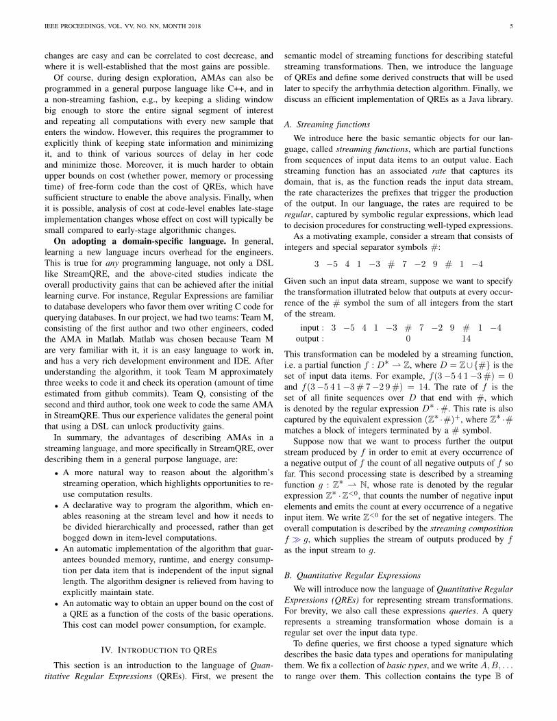
The heart has two upper chambers called the atria andtwo lower chambers called the ventricles (see Fig. 1) Thesynchronized contractions of atria and ventricles assure anadequate supply of oxygenated blood to the rest of the body.This contraction is driven by electrical activity in the heart,which originates in the right atrium, floods the atria first,then conducts down to the ventricles and floods those inturn. The cardiac muscle contracts as it is being traversed bythe electrical wavefront, i.e., as it depolarizes. In a first ap-proximation which is sufficient for understanding AMAs, wemay consider that this contraction is an instantaneous event,and refer to it as an (atrial or ventricular) beat. This normalpattern of electrical activity is referred to as Normal SinusRhythm (NSR), after the sino-atrial node where the electricitynormally originates. Disturbances of NSR are referred to asarrhythmias. They can arise because of structural defects inthe cardiac muscle, like a re-entrant circuit around which theelectrical waveform circulates very fast, or because of irritabletissue that starts to depolarize faster than the sino-atrial node.

Shock Coils

Right Ventricular Electrode

Left AtriumLeft VentricleRight AtriumRight Ventricle

ICD

Can (Shock) Electrode

Atrial Signal

VentricularSignal

ShockSignal

AtrialSensed Event (AS)

VentricularSensed Event (VS)

AS ASVS VS

Right Atrium Electrode

Sense

Therapy

Fig. 1: ICD and its connection to the heart

Ventricular Tachycardia (VT) is an example of an arrhythmiaoriginating in the ventricles, in which the ventricles depolarizeat a very high rate and effectively drive the rhythm. Thishigh rate of depolarization doesn’t give enough time for themuscle to contract and relax properly, which can result ininsufficient blood supply. If the VT is sustained, or degeneratesinto Ventricular Fibrillation (VF) (Fig. 2), it is fatal within aminute. An abnormally fast heart rate that originates in theatria and/or the conduction system above the ventricles isreferred to as a Supra-ventricular Tachycardia (SVT). An SVTcauses patient discomfort but is not fatal in the short-term anddoes not require device treatment. Most fast arrhythmias fallunder these two categories: VT or SVT.

B. Implantable devices

Two types of implantable devices monitor a heart’s rhythmcontinusouly to detect abnormally fast arrhythmias, aka tachy-cardias. The first is Implantable Cardioverter Defibrillators(ICDs). An ICD is inserted under the pectoral muscles, andhas one or two leads that are directly implanted in the cardiacchambers, and through which it measures local electricalactivity - see Fig. 1. The measured signals are known aselectrograms, or EGMs, and are termed ‘atrial’ or ‘ventricular’depending on the chamber where they are measured1. SeeFig. 3. An ICD uses EGMs to distinguish a wide range oftachycardias. If it detects a potentially fatal tachycardia, thenit delivers therapy to the heart in the form of either low-energy

1In this paper, we will ignore the so-called ‘shock EGM’ as it will not beused in describing arrhythmia monitoring algorithms.


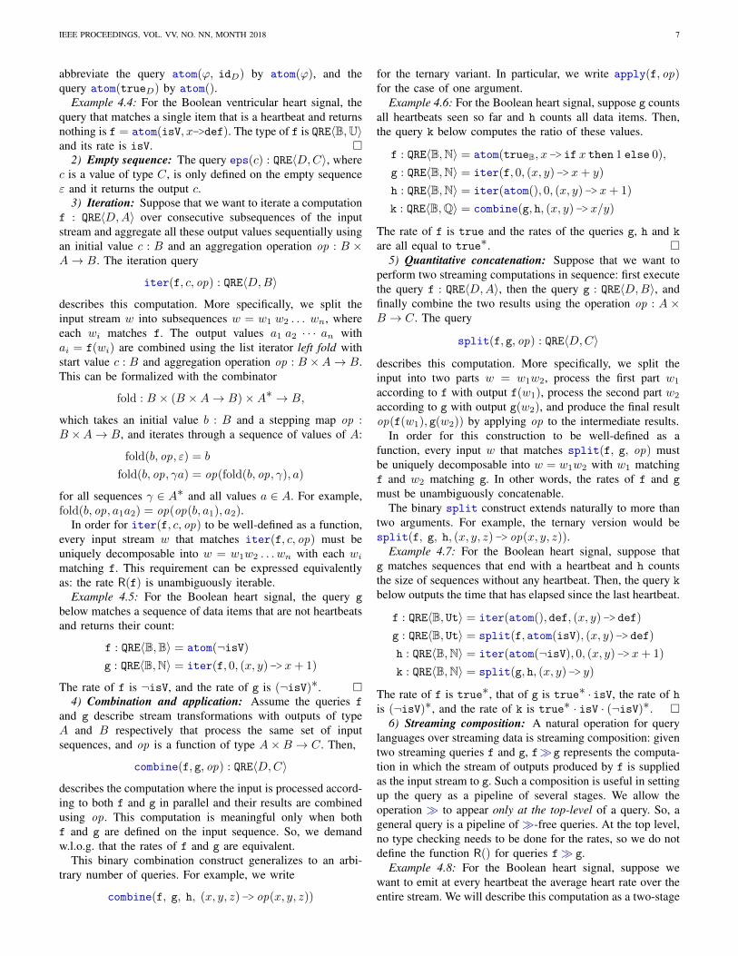
Fig. 2: Electrical activity during Normal Sinus Rhythm (NSR) and Ventricular Fibrillation (VF). The color scale runs from blue = reststate to red = excited (aka depolarized) state. (Colors in digital version). In the top left, the ventricles are shown from two different angles,during a phase of NSR. The ventricles are fully exicted. The bottom left panel shows a later phase of the same beat, where the ventriclesare progressively relaxing, starting with the apex (the pointed tip of the heart). This orderly propagation ensures adequate muscle contractionand blood flow. Three surface ECGs are shown beneath the left column, with red bars indicating the timing of the two snapshots. Note theperiodic pattern. The right column shows two snapshots during VF (earlier snapshot on top). Note the disorganized nature of the electricalactivity, wavefront breakup, and the multiple regions of depolarization. Note also the change in the surface ECG from periodic and regular(early on) to disorganized. The AMA reads two such signals (obtained, however, intra-cardially and not from the surface) and tries to detectfibrillation. [Snapshots obtained from video of a simulation of the ventricles at UCLA, courtesy of Luigi Perotti [19]]

0 1000 2000 3000 4000 5000 6000

-1000

-500

0

500

1000

0 1000 2000 3000 4000 5000 6000

-1

-0.5

0

0.5

1

0 1000 2000 3000 4000 5000 6000

-200

0

200

400

600

ATRIAL

ATRIAL BOOLEAN

VENTRICULAR BOOLEAN

VENTRICULAR

Fig. 3: EGMs (top and bottom panels) and corresponding booleanbeat signals (middle) during atrial tachycardia. Beats correspond topeaks in the EGMs.

pacing sequences or (possibly more than one) very high-energyshock. Either way, the goal of the therapy is to stop the currentrhythm and allow a normal rhythm to start. VTs and SVTs canshare similar heart rates and other characteristics, so an SVTcan be mis-diagnosed as a VT. This is problematic becauseshock therapy used to stop a VT can deliver between 30-60Joules of energy at around 700 Volts in under 15ms [20],directly to the heart, which is very painful to the patient2, and

2Patients compare the shock to a “horse kicking you in the chest”.

has been shown to increase morbidity [21]. Therefore, one ofthe biggest challenges for ICDs is to discriminate between VFand sustained VT that typically requires a shock, and SVT thattypically should not be shocked [22]. This paper will presentone particular ICD AMA in detail in Section V.

The second type of device that monitors tachycardias is theInsertable Loop Recorder (ILR) (also known as ImplantableCardiac Monitor). An ILR is a small device (the smallest ILRon the market is smaller than a key) that is inserted sub-cutaneously, and monitors surface ECG signals. It uses thesesignals to compute a number of long- and short-term statisticsof the rhythm, and in particular to detect Atrial Fibrillation(AF) episodes. AF is an abnormally fast and disorganizedatrial rhythm that can lead to fainting spells, and which, inthe long term, contributes to blood clot formation. These clotscan cause a stroke upon reaching the brain. The ILR doesnot have any therapeutic functions, but only monitors theheart rhythm. As an example, Biotronik’s BioMonitor [23]calculates and stores the following daily quantities, in a slidingwindow of 240 days where the oldest day drops out of thewindow. The quantities include 1) the average daily heartrate, 2) the daily minimum average heart rate, where theaverages are calculated over consecutive blocks of 10 mins inthe day, 3) daily heart rate variability, defined as the standarddeviation of the sliding 5-minute averages, and 4) the ratehistogram, where each heartbeat is binned into bins of width


10 beats-per-minute (bpm). In addition, the BioMonitor willtake consecutive windows of n beats and count the number ofcycle lengths that fall below a fixed value in each window.

Remote continuous monitoring has recently been shownto improve treatment outcomes [24] and to reduce time-to-treatment for patients with atrial tachycardia burden [25], so itis important to develop algorithms that can monitor over longerperiods of time and/or compute more advanced statistics thatcan better detect the arrhythmia burden.

C. Device measurement: from real-valued to boolean signal

Formally, an EGM is a uniformly-sampled, discrete-timereal-valued bounded signal. An EGM signal can be char-acterized by the timing of beats that produced it, and themorphology of the signal itself. To detect the beat timing (i.e.,when the chamber is contracting), the peaks of the EGM aredetected [26]. The output of peak detection is a discrete-timeboolean signal, where a 1 indicates a beat. See Fig. 3. Beattiming is crucial to an arrhythmia’s detection, since it is usedin all discriminators.

The ‘morphology’ refers to the shape of the EGM. The so-called ‘shock’ EGMs during an atrially-driven rhythm lookdifferent from the shock EGMs during a ventricularly-drivenrhythm. The ICD uses this to help it determine whether thecurrent arrhythmia is an SVT or VT. In this paper, and in orderto keep the exposition simple, we will only work with the beatsignal, i.e., the boolean signal produced by peak detection onthe local atrial and ventricular channels, as shown in Fig. 3.

III. STREAMING ALGORITHMS FOR ARRHYTHMIADETECTION

An AMA is naturally viewed as a pipeline of streamingalgorithms, where each node of the pipeline performs astreaming calculation on its input signal, and passes its outputsignal to the next node. So what is a streaming algorithm?And why view arrhythmia monitors as streaming algorithms?The main characteristics of a streaming algorithm are thatit views its input as a sequence, or stream, of items fromsome data domain, arriving one at a time. It gets to processeach item only once, after which it discards it and moves onto the next item in the input stream. After processing eachitem, the algorithm produces an output value (which mightalso be null). A streaming algorithm has limited memoryavailable (much smaller than the length of the stream which,for practical purposes, may be regarded as infinite), andlimited processing time. Section IV gives several examplesof streaming calculations.

The following considerations, which govern the design andexecution of an AMA, establish the suitability of the streamingmodel of calculation for AMA. First, an AMA’s input is auniformly sampled discrete-time electrical signal that arrivesin real-time, one sample at a time, and thus can be viewedas a stream. Second, when running on an ICD, the AMAhas a delay constraint. Namely, not much time must elapsebetwen the onset of a fatal VT and the moment that the AMAdetects it, because this delays the delivery of therapy. Thisrequirement translates directly into a requirement of small

processing time per item of the input signal, which is a keyconstraint on streaming algorithms. Third, ICDs and ILRsshare a power consumption concern. Indeed, power is themain non-functional design factor for these devices. Evenfor today’s ICDs, which can have a battery life between7 and 11 years, an additional 3 months of battery life arestill worth pursuing [27], since they can mean the differencebetween having to surgically replace the ICD or not. Becausemost ICD and ILR recipients are older patients with healthcomplications [28], it is desirable to prolong battery life andreduce the likelihood of a replacement [27]. The power inan ICD is consumed by the monitoring algorithms, the shocktherapy, and the pacing therapy. Although shocks are the singlemost power-hungry event, over an average device’s lifetime,they will only consume 3% of the battery, and it is exceedinglyrare that they consume more than 36% [29]. The rest is sharedbetween pacing and monitoring. Thus it is important to reducethe power cost of monitoring. For ILRs, because they do nothave any therapeutic functions, most of the power is consumedby monitoring. Thus an AMA has a more general small cost-per-item constraint.

If AMAs are viewed as streaming algorithms, then itfollows that they are best programmed using a streamingprogramming language. That is, a language that is expresslydesigned and optimized for describing streaming algorithmsand automatically generating efficient code from the programdescription. Indeed, it is important to note the productivitygains achievable by using a Domain Specific Language (DSL).It is generally agreed that programming in a DSL results ingreater productivity for the development teams producing thesoftware - see, e.g., [30] and [31] where development timereductions of 5-7x are routinely reported. During the designexploration stage when AMAs are developed, tweaked andcompared, it is helpful to program in a language that allowshigh-level reasoning about the stream as the basic object ofmanipulation and easy capture of patterns in the stream.

The StreamQRE language [18], [6] permits such a declar-ative way of programming. StreamQRE (pronounced ‘streamquery’) allows the developer to create Quantitative RegularExpressions (QREs), which are a quantitative extension ofregular expressions. A QRE declares how the stream shouldbe divided up (by matching against a regular expression) andwhich arbitrary operations should be executed on the match-ing pieces. Similarly to regular expressions, QREs can becombined using quantitative extensions of regular combinatorsto form more complex computations. QREs are describedin detail in the next section. QREs also provide theoreticalguarantees on the memory, time and energy consumed toprocess a data item by the resulting algorithm. Specifically, aQRE has per-item memory and time complexities and energyconsumption that are independent of the length of the stream,and depend only on the size of the query. Thus, a QREprogram automatically gives a baseline implementation withconstant cost per data item. One also automatically gets astatic upper bound on the per-item cost of a QRE. This allowsa cost comparison to choose between similarly-performingalgorithms. Such early feedback on cost allows early designexploration, at a point in the design cycle where algorithmic


changes are easy and can be correlated to cost decrease, andwhere it is well-established that the most gains are possible.

Of course, during design exploration, AMAs can also beprogrammed in a general purpose language like C++, and ina non-streaming fashion, e.g., by keeping a sliding windowbig enough to store the entire signal segment of interestand repeating all computations with every new sample thatenters the window. However, this requires the programmer toexplicitly think of keeping state information and minimizingit, and to think of various sources of delay in her codeand minimize those. Moreover, it is much harder to obtainupper bounds on cost (whether power, memory or processingtime) of free-form code than the cost of QREs, which havesufficient structure to enable the above analysis. Finally, whenit is possible, analysis of cost at code-level enables late-stageimplementation changes whose effect on cost will typically besmall compared to early-stage algorithmic changes.

On adopting a domain-specific language. In general,learning a new language incurs overhead for the engineers.This is true for any programming language, not only a DSLlike StreamQRE, and the above-cited studies indicate theoverall productivity gains that can be achieved after the initiallearning curve. For instance, Regular Expressions are familiarto database developers who favor them over writing C code forquerying databases. In our project, we had two teams: Team M,consisting of the first author and two other engineers, codedthe AMA in Matlab. Matlab was chosen because Team Mare very familiar with it, it is an easy language to work in,and has a very rich development environment and IDE. Afterunderstanding the algorithm, it took Team M approximatelythree weeks to code it and check its operation (amount of timeestimated from github commits). Team Q, consisting of thesecond and third author, took one week to code the same AMAin StreamQRE. Thus our experience validates the general pointthat using a DSL can unlock productivity gains.

In summary, the advantages of describing AMAs in astreaming language, and more specifically in StreamQRE, overdescribing them in a general purpose language, are:

• A more natural way to reason about the algorithm’sstreaming operation, which highlights opportunities to re-use computation results.

• A declarative way to program the algorithm, which en-ables reasoning at the stream level and how it needs tobe divided hierarchically and processed, rather than getbogged down in item-level computations.

• An automatic implementation of the algorithm that guar-antees bounded memory, runtime, and energy consump-tion per data item that is independent of the input signallength. The algorithm designer is relieved from having toexplicitly maintain state.

• An automatic way to obtain an upper bound on the cost ofa QRE as a function of the costs of the basic operations.This cost can model power consumption, for example.

IV. INTRODUCTION TO QRES

This section is an introduction to the language of Quan-titative Regular Expressions (QREs). First, we present the

semantic model of streaming functions for describing statefulstreaming transformations. Then, we introduce the languageof QREs and define some derived constructs that will be usedlater to specify the arrhythmia detection algorithm. Finally, wediscuss an efficient implementation of QREs as a Java library.

A. Streaming functions

We introduce here the basic semantic objects for our lan-guage, called streaming functions, which are partial functionsfrom sequences of input data items to an output value. Eachstreaming function has an associated rate that captures itsdomain, that is, as the function reads the input data stream,the rate characterizes the prefixes that trigger the productionof the output. In our language, the rates are required to beregular, captured by symbolic regular expressions, which leadto decision procedures for constructing well-typed expressions.

As a motivating example, consider a stream that consists ofintegers and special separator symbols #:

3 −5 4 1 −3 # 7 −2 9 # 1 −4

Given such an input data stream, suppose we want to specifythe transformation illutrated below that outputs at every occur-rence of the # symbol the sum of all integers from the startof the stream.

input : 3 −5 4 1 −3 # 7 −2 9 # 1 −4output : 0 14

This transformation can be modeled by a streaming function,i.e. a partial function f : D∗ ⇀ Z, where D = Z∪{#} is theset of input data items. For example, f(3−5 4 1−3 #) = 0and f(3−5 4 1−3 # 7−2 9 #) = 14. The rate of f is theset of all finite sequences over D that end with #, whichis denoted by the regular expression D∗ ·#. This rate is alsocaptured by the equivalent expression (Z∗ ·#)+, where Z∗ ·#matches a block of integers terminated by a # symbol.

Suppose now that we want to process further the outputstream produced by f in order to emit at every occurrence ofa negative output of f the count of all negative outputs of f sofar. This second processing state is described by a streamingfunction g : Z∗ ⇀ N, whose rate is denoted by the regularexpression Z∗ ·Z<0, that counts the number of negative inputelements and emits the count at every occurrence of a negativeinput item. We write Z<0 for the set of negative integers. Theoverall computation is described by the streaming compositionf � g, which supplies the stream of outputs produced by fas the input stream to g.

B. Quantitative Regular Expressions

We will introduce now the language of Quantitative RegularExpressions (QREs) for representing stream transformations.For brevity, we also call these expressions queries. A queryrepresents a streaming transformation whose domain is aregular set over the input data type.

To define queries, we first choose a typed signature whichdescribes the basic data types and operations for manipulatingthem. We fix a collection of basic types, and we write A,B, . . .to range over them. This collection contains the type B of


boolean values, and the unit type U whose unique inhabitantis denoted by def. It is also closed under the cartesian productoperation × for forming pairs of values. Typical examples ofbasic types are the natural numbers N, the integers Z, therationals Q, and the real numbers R. We write a : A to meanthat a is of type A. For example, we have def : U.

We also fix a collection of basic operations on the basictypes, for example the k-ary operation op : A1×· · ·×Ak → B.The identity function on D is written as idD : D → D, andthe operations π1 : A × B → A and π2 : A × B → Bare the left and right projection respectively. We assume thatthe collection of operations contains all identities and projec-tions, and is closed under pairing and function composition.To describe derived operations we use a variant of lambdanotation that is similar to Java’s lambda expressions [32]. Thatis, we write (A x) -> t(x) to mean λx:A.t(x), which is an(anonymous) function that takes an argument x of type A andreturns the value t(x). We write (A x, B y, C z)->t(x, y, z)to mean λx:A, y:B, z:C.t(x, y, z). For example, the identityfunction on D is (D x)->x, the left projection on A× B is(A x, B y)->x, the right projection on A×B is (A x, B y)->y, and (D x)->def is the unique function from D to U. Wewill typically use lambda expressions in the context of queriesfrom which the types of the input variables can be inferred,so we will omit the types as in (x, y)->x.

For every basic type D, assume that we have fixed acollection of atomic predicates, so that the satisfiability oftheir Boolean combinations (built up using the Boolean op-erations: and, or, not) is decidable. We write ϕ : D → Bto indicate that ϕ is a predicate on D, and we denote bytrueD : D → B the predicate that is always true. Thepredicate ((Z x) -> x > 0) : Z → B is true of the strictlypositive integers.

Example 4.1: We consider a Boolean ventricular heartsignal, where the data items are values of type B = {0, 1}.A value 1 indicates a ventricular contraction of the heart, anda value 0 indicates the absence of a contraction. The signalis sampled uniformly with a sampling rate of f Hz. Thepredicates ¬isV and isV test if a Boolean value is zero orone respectively. �

For a type D, we define the set of symbolic regularexpressions over D [33], denoted RE〈D〉, with the grammar:

r ::= ϕ | [predicate on D]ε | [empty sequence]r t r | [nondeterministic choice]r · r | [concatenation]

r∗ [iteration].

The concatenation symbol · is sometimes omitted, that is, wewrite rs instead of r · s. The expression r+ (iteration at leastonce) abbreviates r · r∗. We write r : RE〈D〉 to indicate the ris a regular expression over D. Every expression r : RE〈D〉 isinterpreted as a set JrK ⊆ D∗ of finite sequences over D:

JϕK , {d ∈ D | ϕ(d) is true}

and the rest of the regular construct have their usual inter-pretations. Two expressions are said to be equivalent if theydenote the same language.

Example 4.2: The symbolic regular expression (¬isV)∗·isVdenotes sequences of samples that contain a single ventricularbeat (contraction) at the end. �

A string can be matched efficiently against a regular ex-pression if there’s only one way in which it could match theexpression. Intuitively, this reduces the number of possiblematches that have to be kept track of. The notion of unam-biguity for regular expressions [34] is a way of formalizingthe requirement of uniqueness of parsing. The languages L1,L2 are said to be unambiguously concatenable if for everyword w ∈ L1 · L2 there are unique w1 ∈ L1 and w2 ∈ L2

with w = w1w2. The language L is said to be unambiguouslyiterable if for every word w ∈ L∗ there is a unique integern ≥ 0 and unique wi ∈ L with w = w1 · · ·wn. The definitionsof unambiguous concatenability and unambiguous iterabilityextend to regular expressions in the obvious way. Now, aregular expression is said to be unambiguous if it satisfiesthe following:

1) For every subexpression e1 t e2, e1 and e2 are disjoint.2) For every subexpression e1 · e2, e1 and e2 are unambigu-

ously concatenable.3) For every subexpression e∗, e is unambiguously iterable.Example 4.3: Consider the finite alphabet Σ = {a, b}. The

regular expression r = (a t b)∗b(a t b)∗ denotes the set ofsequences with at least one occurrence of b. It is ambiguous,because the subexpressions (a t b)∗b and (a t b)∗ are notunambiguously concatenable: the word w = ababa matches r,but there are two different splits w = ab ·aba and w = abab ·athat witness the ambiguity of parsing. The regular expressionsa∗b(atb)∗ and (atb)∗ba∗ are both equivalent to r, and theyare unambiguous. �Checking whether a regular expression is unambiguous canbe done in polynomial time. For the case of symbolic regularexpressions this results still holds, under the assumption thatsatisfiability of the predicates can be decided in unit time [35].

After these preliminaries, we now define quantitative regularexpressions, or queries, recursively. Informally, a query f is asymbolic regular expression, called the rate of f and writtenR(f), with a way to compute quantities over the strings thatmatch the expression. The rate denotes the domain of thetransformation that f represents. The definition of the querylanguage has to be given simultaneously with the definition ofrates (by mutual induction), since the query constructs havetyping restrictions that involve the rates. We annotate a queryf with a type QRE〈D,C〉 to denote that the input stream haselements of type D and the outputs are values of type C.

1) Atomic queries: The basic building blocks of queries areexpressions that describe the processing of a single data item.Suppose ϕ : D → B is a predicate over the data item type Dand op : D → C is an operation from D to the output type C.Then, the atomic query atom(ϕ, op) : QRE〈D,C〉, with rateϕ, is defined on single-item streams that satisfy the predicateϕ. The output is the value of op on the input element.

Notation: It is very common for op to be the identityfunction, and ϕ to be the always-true predicate. So, we


abbreviate the query atom(ϕ, idD) by atom(ϕ), and thequery atom(trueD) by atom().

Example 4.4: For the Boolean ventricular heart signal, thequery that matches a single item that is a heartbeat and returnsnothing is f = atom(isV, x->def). The type of f is QRE〈B,U〉and its rate is isV. �

2) Empty sequence: The query eps(c) : QRE〈D,C〉, wherec is a value of type C, is only defined on the empty sequenceε and it returns the output c.

3) Iteration: Suppose that we want to iterate a computationf : QRE〈D,A〉 over consecutive subsequences of the inputstream and aggregate all these output values sequentially usingan initial value c : B and an aggregation operation op : B ×A→ B. The iteration query

iter(f, c, op) : QRE〈D,B〉describes this computation. More specifically, we split theinput stream w into subsequences w = w1 w2 . . . wn, whereeach wi matches f. The output values a1 a2 · · · an withai = f(wi) are combined using the list iterator left fold withstart value c : B and aggregation operation op : B ×A→ B.This can be formalized with the combinator

fold : B × (B ×A→ B)×A∗ → B,

which takes an initial value b : B and a stepping map op :B ×A→ B, and iterates through a sequence of values of A:

fold(b, op, ε) = b

fold(b, op, γa) = op(fold(b, op, γ), a)

for all sequences γ ∈ A∗ and all values a ∈ A. For example,fold(b, op, a1a2) = op(op(b, a1), a2).

In order for iter(f, c, op) to be well-defined as a function,every input stream w that matches iter(f, c, op) must beuniquely decomposable into w = w1w2 . . . wn with each wi

matching f. This requirement can be expressed equivalentlyas: the rate R(f) is unambiguously iterable.

Example 4.5: For the Boolean heart signal, the query g

below matches a sequence of data items that are not heartbeatsand returns their count:

f : QRE〈B,B〉 = atom(¬isV)

g : QRE〈B,N〉 = iter(f, 0, (x, y)->x+ 1)

The rate of f is ¬isV, and the rate of g is (¬isV)∗. �4) Combination and application: Assume the queries f

and g describe stream transformations with outputs of typeA and B respectively that process the same set of inputsequences, and op is a function of type A×B → C. Then,

combine(f, g, op) : QRE〈D,C〉describes the computation where the input is processed accord-ing to both f and g in parallel and their results are combinedusing op. This computation is meaningful only when bothf and g are defined on the input sequence. So, we demandw.l.o.g. that the rates of f and g are equivalent.

This binary combination construct generalizes to an arbi-trary number of queries. For example, we write

combine(f, g, h, (x, y, z)-> op(x, y, z))

for the ternary variant. In particular, we write apply(f, op)for the case of one argument.

Example 4.6: For the Boolean heart signal, suppose g countsall heartbeats seen so far and h counts all data items. Then,the query k below computes the ratio of these values.

f : QRE〈B,N〉 = atom(trueB, x->if x then 1 else 0),

g : QRE〈B,N〉 = iter(f, 0, (x, y)->x+ y)

h : QRE〈B,N〉 = iter(atom(), 0, (x, y)->x+ 1)

k : QRE〈B,Q〉 = combine(g, h, (x, y)->x/y)

The rate of f is true and the rates of the queries g, h and k

are all equal to true∗. �5) Quantitative concatenation: Suppose that we want to

perform two streaming computations in sequence: first executethe query f : QRE〈D,A〉, then the query g : QRE〈D,B〉, andfinally combine the two results using the operation op : A ×B → C. The query

split(f, g, op) : QRE〈D,C〉describes this computation. More specifically, we split theinput into two parts w = w1w2, process the first part w1

according to f with output f(w1), process the second part w2

according to g with output g(w2), and produce the final resultop(f(w1), g(w2)) by applying op to the intermediate results.

In order for this construction to be well-defined as afunction, every input w that matches split(f, g, op) mustbe uniquely decomposable into w = w1w2 with w1 matchingf and w2 matching g. In other words, the rates of f and g

must be unambiguously concatenable.The binary split construct extends naturally to more than

two arguments. For example, the ternary version would besplit(f, g, h, (x, y, z)-> op(x, y, z)).

Example 4.7: For the Boolean heart signal, suppose thatg matches sequences that end with a heartbeat and h countsthe size of sequences without any heartbeat. Then, the query k

below outputs the time that has elapsed since the last heartbeat.

f : QRE〈B, Ut〉 = iter(atom(), def, (x, y)->def)

g : QRE〈B, Ut〉 = split(f, atom(isV), (x, y)->def)

h : QRE〈B,N〉 = iter(atom(¬isV), 0, (x, y)->x+ 1)

k : QRE〈B,N〉 = split(g, h, (x, y)-> y)

The rate of f is true∗, that of g is true∗ · isV, the rate of his (¬isV)∗, and the rate of k is true∗ · isV · (¬isV)∗. �

6) Streaming composition: A natural operation for querylanguages over streaming data is streaming composition: giventwo streaming queries f and g, f�g represents the computa-tion in which the stream of outputs produced by f is suppliedas the input stream to g. Such a composition is useful in settingup the query as a pipeline of several stages. We allow theoperation � to appear only at the top-level of a query. So, ageneral query is a pipeline of�-free queries. At the top level,no type checking needs to be done for the rates, so we do notdefine the function R() for queries f� g.

Example 4.8: For the Boolean heart signal, suppose wewant to emit at every heartbeat the average heart rate over theentire stream. We will describe this computation as a two-stage


pipeline. The first stage (query h below) produces a sequenceof natural numbers which correspond to the number of 0’sbetween two consecutive 1’s (heartbeats).

f : QRE〈B,N〉 = iter(atom(¬isV), 0, (x, y)->x+ 1)

g : QRE〈B,N〉 = split(f, atom(isV), (x, y)->x)

h : QRE〈B,N〉 = split(iter(g, def, (x, y)->def),

g, (x, y)-> y)

The rate of f is (¬isV)∗, the rate of g is (¬isV)∗ · isV, andthe rate of h is ((¬isV)∗ · isV)+. The second stage (query n

below) processes a stream of these numbers to compute theaverage heart rate in beats per minute.

k : QRE〈N,N〉 = iter(atom(), 0, (x, y)->x+ y)

l : QRE〈N,N〉 = iter(atom(), 0, (x, y)->x+ 1)

m : QRE〈N,Q〉 = combine(k, l, (x, y)->x/y))

n : QRE〈Q,Q〉 = apply(m, x-> (60 · f)/x)

where f is the sampling rate in Hz. The query m computesthe average number of samples between two consecutiveheartbeats. The top-level query is the pipeline h� n. �

7) Global choice: Given queries f and g of the same typewith disjoint rates r and s, the query or(f, g) applies either for g to the input stream depending on which one is defined.The rate of or(f, g) is the union rts. This choice constructionallows a case analysis based on a global regular property ofthe input stream.

Example 4.9: In our Boolean heart example, suppose wewant to compute a statistic across days, where the contributionof each day is computed differently depending on whether ornot an abnormally short interval between consecutive heart-beats occured or not. Then, we can write a query summarizingthe daily activity with a rate capturing normal days (the oneswithout any short interval) and a different query with a ratecapturing abnormal days, and iterate over their disjoint union.

Consider the stream of interval lengths between consecutiveheartbeats, i.e. the output stream of query h defined in Exam-ple 4.8. We assume that T is the threshold for an abnormallyshort interval between two consecutive heartbeats. Query h

below computes the smallest interval length for sequences withat least one abnormally short interval:

f : QRE〈N,Q〉 = iter(atom(x->x > T ),∞,min)

g : QRE〈N,Q〉 = iter(atom(),∞,min)

h : QRE〈N,Q〉 = split(f, atom(x->x ≤ T ), g,min)

The rate of f is (x > T )∗, the rate of g is true∗, and the rateof h is (x > T )∗ · (x ≤ T ) · true∗. Query m below computesthe average interval length for sequences with no abnormallyshort interval:

k : QRE〈N,N〉 = iter(atom(x->x > T ), 0, (x, y)->x+ y)

l : QRE〈N,N〉 = iter(atom(x->x > T ), 0, (x, y)->x+ 1)

m : QRE〈N,Q〉 = combine(k, l, (x, y)->x/y)

The rates of k, l and m are all equal to (x > T )∗. The top-levelquery is then or(h, m). �

C. Derived constructs

The core language of Section IV-B is expressive enough todescribe many common stream transformations. We presentbelow several derived constructs.

1) Matching without output: Suppose r is an unambiguoussymbolic regular expression over the data item type D. Thequery match(r), whose rate is equal to r, does not produceany output when it matches. This is essentially the same asproducing def as output for a match. The match constructcan be encoded as follows:

match(ϕ) , atom(ϕ, x->def)

match(r1 t r2) , or(match(r1), match(r2))

match(r1 · r2) , split(match(r1), match(r2), (x, y)->def)

match(r∗) , iter(match(r), def, (x, y)->def)

An easy induction establishes that R(match(r)) = r.2) “Until” Iteration: Suppose that φ and ψ are disjoint

predicates on the input data type D, the function op : C×D →C is an aggregation operation, and c : C is the initialaggregate. The query iterUntil(φ, ψ, c, op) aggregates asequence of data items that satisfy φ and stops when an itemthat satisfies ψ is found. It is encoded as:

iterUntil(φ, ψ, c, op) , split(iter(atom(φ), c, op),

atom(ψ), (x, y)->x)

The query has type QRE〈D,C〉 and rate φ∗ · ψ.3) Stream Annotation: Suppose that the input stream has

items of type D, f is a query of type QRE〈D,C〉, and wewant to produce an output stream with items of type E in thefollowing way: when the query f produces an output (uponconsumption of the input stream) apply op2 : D×C → E tothe last input element and its output to get the final result,and when the query f is undefined apply op1 : D → Eto the last input element. This computation is described bythe query annt(f, op1, op2) : QRE〈D,E〉 with rate D+. Thisannotation query can be encoded using the regular constructsof Section IV-B, but the encoding is complex and inefficient,so we provide a custom efficient implemenation.

a) Tumbling windows: The term tumbling windows isused to describe the splitting of the stream into contiguousnon-overlapping subsequences [36]. Suppose we want to de-scribe the streaming function that iterates f at least once andreports the result given by f at every match. The followingquery expresses this behavior:

iterLast(f) , split(match(R(f)∗), f, (x, y)-> y).

The rate of iterLast(f) is equal to R(f)+.4) Efficient Sliding Windows: Suppose we want to apply

the query f : QRE〈D,A〉 to consecutive nonoverlapping partsof the input, and efficiently aggregate the intermediate resultsover a sliding window of size W . That is, the W most recentoutput values of f are aggregated to produce the final output.The aggregation is described by an initial aggregate c : B andthree functions: an insertion operation ins : B × A → Bdescribes how to add a new value of type A to the aggregate(of type B), the removal operation rmv : B×A→ B describes


// Process a single value: rate DoubleQRe<Double, Double> f =

Q.atomic(x -> true, x -> x);

// Sum of sequence of values: rate Double*QRe<Double, Double> sum =

Q.iter(f, 0.0, (x,y) -> x+y);

// Length of sequence of values: rate Double*QRe<Double, Long> count =

Q.iter(f, 0L, (x,y) -> x+1);

// Average of sequence of values: rate Double*QRe<Double, Double> avg =

Q.combine(sum, count, (x,y) -> x/y);

Iterator<Double> stream = ... // input stream

// evaluator for the queryEval<Double, Double> e = avg.getEval();

// execution loopDouble output = e.start();// e.start() returns null, if undefinedwhile (stream.hasNext()) {

Double d = stream.next();output = e.next(d);// e.next(d) returns null, if undefined

}

Fig. 4: StreamQRE Library in Java: Computing the average ofa sequence of values.

how to remove a value from the aggregate, and the finalizationoperation op : B → C computes the final result from theaggregate. This computation is described by the query

wnd(f,W, c, ins, rmv, op) : QRE〈D,C〉,whose rate is equal to R(f)+. This query can be encoded usingthe regular constructs of Section IV-B and an additional datatype for FIFO queues (in order to maintain the buffer of valuesof type A that are currently in the active window).

D. A Java Library of QREsStreamQRE has been implemented as a Java library [18]

in order to facilitate the easy integration with user-definedtypes and operations. The implementation covers all the coreconstructs of Section IV-B, and also provides optimizationsfor the derived constructs of Section IV-C (matching withoutoutput, “until” iteration, stream annotation, etc.).

Figure 4 gives a simple example that illustrates how toprogram with the StreamQRE Java library. The query avgdescribes the computation of the average of a sequence ofvalues of type Double. The method getEval, which standsfor “get evaluator”, is used to obtain an object that encapsu-lates the evaluation algorithm for the query. On this evaluatorobject, the methods start and next are used to initialize thealgorithm and consume data items respectively.

V. AN ICD ARRHYTHMIA MONITORING ALGORITHM

We now describe in details an Arrhythmia MonitoringAlgorithm (AMA) found in one of the ICDs on the market

Three consecutive short intervals &8/10 intervals are short

Begin Duration (1 to 5sec)

6 out of every 10 intervals are short No Therapy

V rate > A rate + 10 bpm Therapy

Afib Rate &V rate unstable &Onset is gradual

Therapy

No Therapy

YES

NO

YES

NO

NO

YES

Duration

Fig. 5: Boston Scientific discrimination algorithm

today [17]. All ICD AMAs on the market today take the formof a decision tree, such as the one in Fig. 5. Each node inthe tree is a discriminator, which computes one feature ofthe input signal and decides, on its basis, how to branch.Thus, each discriminator returns a decision, Yes or No. Wechose to present this particular AMA because variants onits discriminators can be found in the AMAs of all deviceson the market. For example, all devices measure averageheart rate, compare atrial and ventricular rates, measure ratevariability, onset of arrhythmia, etc. The differences are in howvariability is defined (variance or sum of absolute differences,for example), the size of windows for computing quantities,the way they are combined in the decision tree, etc.

A. Discriminators

Recall that the input to the AMA is a discrete-time booleansignal, which is obtained by running a peak detector onthe discrete-time real-valued EGM signal. The peak detectoroutputs a 1 at peaks, and 0 otherwise. The signals we workwith in this paper have a sampling period of 1ms. Formally,let B = {0, 1}. At every time t ∈ N, the AMA receives a dataitem s of the following form

s = (V,A, t) ∈ D := B× B× N (1)

where V = 1 indicates there is a ventricular beat at time t(and V = 0 indicates that there is not). Similarly for A. We


Fig. 6: Input stream from one channel. Measured electrogram (top figure) and corresponding Boolean stream (bottom figure).In the Boolean stream, spikes represent beats, and Ik is an interval of time between beats. Duration is a fixed time period,here set to 5 seconds.

will find the need to refer to the ventricular boolean signalseparately, and we write V ∈ B∗ to denote it. It will also becalled the ventricular channel. Similarly, A ∈ B∗ is the atrialchannel. See Fig. 6. Given an item s, the function call s.Vreturns its first element; similarly for s.A and s.t.

An (atrial or ventricular) interval in a given channel is theinterval of time between two consecutive beats. Its length isdenoted by I , and is always an integer measured in millisec-onds (ms). The average (atrial or ventricular) rate is the inverseof the average interval length.

The decision tree of the AMA we describe is shown inFig. 5. It is made up of the following discriminators.

1) Three Consecutive Short Intervals: Three consecutiveshort intervals are required to initiate rhythm analysis, asthey indicate a potentially accelerating rhythm. Therefore, thisdiscriminator checks if three consecutive intervals are shorterthan some pre-specified threshold Tcsi. Referring to Fig. 6:

CSI := (I5 < Tcsi) ∧ (I6 < Tcsi) ∧ (I7 < Tcsi) (2)

2) 8/10 Short Intervals: A rhythm that becomes fast for afew beats then slows down again is not fatal and so should notcause therapy to be delivered. To estimate whether the currentrhythm is sustained, this discriminator checks whether 8 out of10 intervals are shorter than some threshold T8/10. Referringto Fig. 6:

Short8outof10 := |{Ik : 5 ≤ k ≤ 14, Ik < T8/10}| ≥ 8 (3)

3) Sudden Onset: Ventricular Fibrillation (VF), which isfatal, usually occurs suddenly, whereas a tachycardia that ac-celerates gradually is usually non-fatal. The Onset discrimina-tor quantifies the suddenness of tachycardia onset as follows. Itoperates in two steps, which process a window of 2m intervals.To help explain this discriminator using Fig. 6, we will assumem = 4. In the first step, it detects the ventricular beat inthe first 4 intervals (I1, . . . , I4) at which the interval lengthdecreased the most. This is the pivot beat. If the amount of

decrease is greater than some threshold, Step I declares Onset.In the second step, the algorithm computes the differences be-tween the average of 4 pre-pivot beats ((I1+ . . .+I4)/4 := µ)and each of 4 post-pivot beats (I5, . . . , I8). I.e., it computesd5 = µ−I5, . . . , d8 = µ−I8. If at least 3 of these 4 differencesd5, . . . , d8 is greater than a threshold, Step II declares Onset. Ifboth stages declare Onset, the discriminator declares SuddenOnset. In our implementation, we simplify things by takingthe pivot to be the middle beat in the window of 2m = 8intervals. So SuddenOnset is computed as:

SO-StepI := Ipost−pivot < α · Ipre−pivot (4)SO-StepII := |{dk : dk > To2}| ≥ 3 (5)

SuddenOnset := SO-StepI ∧ SO-StepII

When both Three Consecutive Short Intervals and 8/10 ShortIntervals match, then a Duration is started. A Duration is afixed-length time period (e.g., 5sec) during which the algo-rithm will continue to monitor the rhythm to see whether thearrhythmia is sustained, or it slows down and dies out. Inthe latter case, no therapy is delivered. See Fig. 6. DuringDuration, the following four discriminators are evaluated.

4) A/V Rate Comparison: If the ventricles have more beatsthan the atria, this is an almost sure sign that the arrhythmiais ventricular in origin (i.e., the ventricles are driving the atriaand not the other way around). This discriminator comparesthe average ventricular heart rate rV with the average atrialheart rate rA, where the average is computed over the last 10intervals in the Duration window:

AVRate := rV > rA + 10bpm

5) Sliding 6/10: Sometimes an arrhythmia terminates onits own, which is preferable to having the device terminate itwith a shock. This discriminator continuously checks whether


6 out of every 10 intervals are short; if any 10 intervals failsthis check, the discriminator declares No Therapy.

Sliding6outof10 := For every 10 intervals I1, . . . , I10|{Ik : Ik < T6/10}| ≥ 6

6) Stability: VF is an unstable rhythm, meaning that theinterval lengths during fibrillation vary greatly. The Stabilitydiscriminator defines rhythm stability as being the variance inventricular intervals’ lengths during Duration. If variance isbelow a threshold Tstab, then the rhythm is deemed stable.With I denoting the average interval length,

Stability :=1

n

n∑

k=1

(Ik − I)2 ≤ Tstab

7) AFib Rate: Atrial Fibrillation (AF) is an atrially-drivenrhythm with a high rate, and is one possible source ofmisclassification for the AMA. To circumvent this issue, thisdiscriminator measures the atrial rate throughout the Duration.As long as at least 4/10 intervals are shorter than the AFthreshold Taf , this discriminator decides that the currentrhythm is in fact AF and therapy should be withheld.

SlidingAFib := For every 10 interval lengths I1, . . . , I10|{Ik : Ik < Taf}| ≥ 4

VI. QRE IMPLEMENTATION OF THE ARRHYTMIAMONITORING ALGORITHM

The QRE implementation of the BSC algorithm of SectionVis divided into four main stages. The first two stages annotatethe input signal with additional information: the lengths ofthe intervals between heartbeats, and some sliding-windowstatistics over them. The annotated stream is passed to thelater stages in order to compute the discriminators for decid-ing whether therapy should be delivered or not. We give ahigh-level overview of each stage in Section VI-A, as wellas more detailed descriptions and QREs implementations inSections VI-B to VI-E.

A. Overview of Implementation Stages

All discriminators described in Section V use the intervallengths between consecutive heartbeats. In order to simplifythe later computations, it is useful to annotate the streamwith this extra information so that it is readily available inthe next processing steps. Similarly, there are some sliding-window statistics that are required for the discriminators “A/VRate Comparison”, “Sliding 6/10” and “AFib Rate”. Thesequantities require looking at the 10 previous intervals to becomputed. The specification of the algorithm is much easierif this information is already present in the stream, whichobviates the need to look back 10 intervals into the past. Thismotivates our design choice to always annotate the stream withthese useful sliding-window statistics.

The ICD’s AMA receives beats from the atrium and theventricle. The input stream consists of data items that are ofthe form shown in (1). The implementation is a multi-stagepipeline, where each stage is a QRE. Each stage feeds its

1 1 1STAGE 0

(1, I) (1, I) (1, I)STAGE 1

(1, I, w10fast, w10sum)(1, I, w10fast, w10sum)

…

STAGE 2

(1, I, w10fast, w10sum, SO, BD)(1, I, w10fast, w10sum, SO, BD)

STAGE 3

THERAPY NO THERAPY

(1, I, w10fast, w10sum)

…

……

……

……

……

(1, I, w10fast, w10sum, SO, BD)

NO THERAPY

Fig. 7: The overall detection algorithm, shown for the ventricularchannel and with the timestamp sequence omitted. The top streamgives the input boolean signal. Streams below it are annotated withthe information in bold font. I = Interval Length, w10fast = numberof last 10 intervals that are short, w10sum = sum of last 10 intervallengths, SO = Sudden Onset flag, BD = Begin Duration flag.

1 1 1

(1, 253) (1, 190) (1, 200)

……

…

I = 253 I = 190

1

I = 200

(1, 260)V0 =

V =

…

Fig. 8: Stage 0 annotates both channels V and A with intervallengths, i.e. the number of 0s between 1s. Here it is shown operatingon the ventricular channel.

output stream to the following stage for further annotationand processing. They are:

• Stage 0: pre-processing stage which annotates the inputstream s with the lengths of the ventricular and atrialintervals. See Figure 8. The output from this stage willbe used in all subsequent stages. Call the output streamof this stage s0.

• Stage 1: augments its input stream s0 with two pieces ofinformation. The first is the total duration of every win-dow of 10 consecutive intervals, in both channels. Thiswill be used for the A/V Rate Comparison discriminator.The second piece of information is the number of short3

intervals in every window of 10 consecutive intervals, inboth channels. This will be used for the Sliding 6/10 andAFib Rate Comparison discriminators. See Figure 9 for

3I.e., those that are shorter than a pre-defined threshold T6/10.


(1, 253) (1, 190) (1, 200)…

(1, 260)V0 = (1, 203)

0 + 1 + … + 1

10 intervals

260 + 253 + … + 190P

IkP(Ik < 255?)

(w10sum, w10short) = (3640, 2)

0 + 1 + … + 1

253 + 242 + … + 200

(w10sum, w10short) = (3580, 3)

1 + 1 + … + 1

241 + 240 + … + 203

(w10sum, w10short) = (3530, 5)

V1 = …, (1,190, 3640, 2), (1, 200, 3580, 3), (1, 203, 3530, 5), …

…

…

Fig. 9: Stage 1, shown acting on the V channel, augments V0 withthe total duration counter w10sum and the short intervals counterw10short, computed over the last 10 intervals. Here, the thresholdT6/10 = 255.

the computation of both quantities on the V channel. Callthe output stream of this stage s1.

• Stage 2: detects the beginning of Duration, the periodof time during which the rhythm is monitored for afixed amount of time to confirm whether a suspectedarrhythmia is indeed sustained and ventricular in ori-gin. For Duration to be declared and monitored, boththe Three Consecutive Short Intervals and 8/10 ShortIntervals discriminators must return Yes. If Duration isinitiated as a result, the input stream s1 is annotatedwith a BD marker to indicate the start of Duration. SeeFig. 10. This stage also computes the Onset discriminatorand annotates the stream with flag SO = 1 if it is met.Call the output stream of this stage s2.

• Stage 3: final stage, has input stream s2. It computesall discriminators in Duration: Stability, Sliding 6/10, AVRate Comparison, and AFib Rate. Based on all these andthe value of Onset, the stage makes a final decision ofTherapy or No Therapy. See Figure 10.

REMARK. Because a QRE describes a streaming algorithm,each of the above stages operates continuously and issues anoutput with every new data item (including ⊥ if the stringso far doesn’t match). So for example, it is possible forStage 2 to declare the start of Duration several times in arow, i.e., to output BD = 1 several times. See Fig. 14 foran example. The first Duration to end in a Therapy decisionin Stage 3 will cause therapy to be scheduled, and the otherDurations in progress are aborted. On the other hand, if the firstDuration does not end in therapy, the subsequent ones continueto be monitored to their conclusion. Thus one importantconsequence of this streaming implementation is that it ispossible for the QRE to track multiple simultaneous potential

…

(1, 190, 3640, 2)V1 =

Three Consecutive

Short Intervals

14 intervals

Sudden Onset I

8/10 Short Intervals

Stability

5 seconds = Duration length

(1, 301, 3500, 9)

Sudden Onset II

BD = 1 (Begin Duration)

SO = 1 (Sudden Onset)

Sliding 6/10 Short Intervals

AV Rate ComparisonAFib Rate

THERAPY

V2 = …, (1, 301, 3500, 9, SO = 1, BD = 1), (1, 257, 3400, 7, 0, 0), …

STAGE 2 Computations

STAGE 3 Computations

V3 = …, THERAPY, THERAPY, NO THERAPY, …

500 350 355 342 350 350 348 342 349 355 325 343 351 341

350 < ↵ · 500

IV =

Ik Tcsi

Ik T8/10 = 350

Fig. 10: Stages 2 and 3. The rectangles show the computed discrimi-nators, and their width covers the part of the input stream used in thecomputation. E.g., “8/10 Short Intervals” uses the 10 intervals aboveits box, while Stability uses all intervals in the Duration window.Downward blue arrows indicate when a quantity is computed. E.g.,the BD marker is computed every 14 intervals. SO and BD areadded to stream V1 to obtain stream V2. The A channel is notshown, though it enters in the calculation of AV Rate Comparisondiscriminator.

arrhythmias. In this way, no potentially fatal arrhythmia ismissed.

We will explain now each stage in detail, and present theprecise implementation in the StreamQRE language. Recall theQRE constructs of Section IV and the type of the input dataitems (1). Some computations are performed in the same wayboth on the atrial and the ventricular channel. In such caseswe will only give the queries that describe the processing ofthe ventricular channel for the sake of brevity.

B. Stage 0: Annotate interval lengths

This stage annotates the stream with heartbeat intervallengths, that is, the lengths of the sequences between twoconsecutive heartbeats. So, the length of an interval of theform 100 · · · 001 is the number of 0s between the 1s. Thiscomputation is performed both for the ventricular and atrialchannel. The regular expression that describes a signal that hasa single heartbeat at the end is 0∗1. The query for computingthe ventricular interval lengths is the following:

lincr = (x, y)->x+ 1, of type N× N→ NintV = iterUntil(¬isV, isV, 0, lincr)

allIntV = iterLast(intV) // rate ((¬isV)∗ · isV)+

annt0V = annt(allIntV, x->x, (x, c)->x[IV := c])

stage0 = annt0V� annt0A


The query intV iterates over the 0s of the ventricular channel(predicate ¬isV) while incrementing a counter until it encoun-ters a 1 (predicate isV). The query allIntV iterates intV overconsecutive nonoverlapping subsequences, thus processing allventricular intervals. The query annt0V annotates the inputelements with the interval values IV calculated by allIntV,and annt0A does the same with the atrial channel. See Fig. 8.Therefore, the output stream s0 from this stage consists ofdata items of the following form:

s0 = (V, IV , A, IA, t) ∈ D0 = (B× N)2 × N (6)

C. Stage 1: Sudden Onset and Short Intervals

The input stream for this stage consists of items of the formshown in (6). In this state, we first calculate the sum of intervallengths over a sliding window that consists of 10 intervals, andwe annotate the stream with this information (see Fig. 9):

blockV = split(match((¬isV)∗), isV, (x, y)-> y.IV )

wndSumV = wnd(blockV, 10, 0, (x, y)->x+ y)

stg1SumV = annt(wndSumV, x->x, (x, c)->x[SumV := c])

The query blockV matches 0∗1 in the ventricular channel andreturns the length of the interval that ends with the matched 1.The query wndSumV executes blockV over a sliding windowof size 10 and accumulates the interval lengths by summingthem up. The query stg1SumV annotates the stream with allthese sliding-window sums.

In the second part of this stage we also calculate the numberof short ventricular intervals over a sliding window of size 10,where “short” is defined as being of length less than T6/10.

shortV = apply(blockV,

x->if (x ≤ T6/10) then 1 else 0)

wndShortV = wnd(shortV, 10, 0, (x, y)->x+ y)

stg1ShortV = annt(wndShortV, x->x,(x, y)->x[ShrtV := c])

The query shortV applies a thresholding operator to theoutput of blockV. As before, shortV is run in a sliding-window fashion using the wnd construct, and the output isannotated onto the stream using annt.

The same two computations are performed on the atrialchannel, but with a different threshold, Tafib , for stg1ShortA.The final query for this state is the streaming composition ofthe above channel-specific computations:

stage1 =

stg1SumV� stg1ShortV� stg1SumA� stg1ShortA

The output stream s1 of this stage consists of items (withre-arrangement) of the following form:

s1 = (V, IV , SumV, ShrtV,A, IA, SumA, ShrtA, t)

∈ D1 = (B× N3)2 × N (7)

D. Stage 2: Sudden Onset and Begin Duration

This stage computes the Sudden Onset discriminator andBegin Duration (BD) marker at every ventricular beat. In orderto do this, the last 14 ventrical intervals I1, I2, . . . , I14 haveto be considered, as shown in Fig. 10.

• The first 4 intervals I1, I2, I3 and I4 are used for Step Iof “Sudden Onset”, defined in (4).

• The next 4 intervals I5, I6, I7 and I8 are used for StepII of “Sudden Onset”, defined in (5).

• The intervals I5, I6, I7 are used for the “Three Consec-utive Intervals” discriminator, defined in (2).

• The last 10 intervals I5, I6, . . . , I14 are used for the “8/10Short Intervals” discriminator, defined in (3).

This stage splits the stream into consecutive intervals, andevaluates all the relevant discriminators over the last 14intervals using the operation opStage2 : N14 → B × B. Theinput to opStage2 is a vector of 14 ventricular interval lengths,and the output is a pair of Boolean values: the first componentindicates the presence of “Sudden Onset” (SO), and the secondcomponent indicates the presence of “Begin Duration” (BD).

sobd = split(blockV, . . . , blockV,

(x1, . . . , x14)-> opStage2 (x1, . . . , x14))

wndsobd = split(match(R(blockV)∗), sobd, π2)

stage2 = annt(wndsobd, x->x,(x, 〈c1, c2〉)->x[SO := c1,BD := c2])

The query sobd : QRE〈D1,B2〉 matches 14 consecutive ven-tricular intervals, and applies the function opStage2 to theirlengths in order to compute the Boolean flags for “SuddenOnset” and “Begin Duration”. This computation is executedin a sliding-window fashion and the output is used to annotatethe stream. The output stream s2 from Stage 2 contains dataitems of the following form:

s2 = (s1,SO ,BD) ∈ D2 = D1 × B2

E. Stage 3: Therapy Decision

This stage uses the four discriminators shown in Fig. 10to make the final decision whether to apply therapy or not.Whenever “Begin Duration” (BD) is detected by the previousstage, the algorithm considers the window of N data itemsfollowing BD, and the discriminators are computed using theinformation contained within this window. For example, if theDuration window is programmed to be 5 seconds, and thesampling rate is 256Hz, then the window contains N = 5 ×256 = 1280 items. The query

stage3 = wnd(atom(), N, 0, ins, rmv, discr)

describes a sliding-window computation that maintains abuffer with all ventricular and atrial beats of the durationperiod. The function ins adds a new item to the buffer, thefunction rmv removes an expiring item from the buffer, andthe operation discr computes the discriminators and the finaltherapy decision using only the items contained in the buffer.


F. Overall AMA Query

The top-level query for this Arrhythmia Monitoring Algo-rithm is the streaming composition of all stages (see Fig. 7):

AMA = stage0� stage1� stage2� stage3.

VII. ILLUSTRATIVE EXAMPLES

A. Sample executions

Two examples will serve to illustrate the details of thequery execution. Fig. 11 shows a Ventricular Fibrillation (VF)EGM signal along with the corresponding boolean beat stream.The results of running stage2 on this signal are presentedin a Fig. 12. At times 12, 572 ms and 12, 811 ms the startof Duration is detected (BD = 1). At the end of the firstinitiated Duration (at 17, 572 ms), the A/V Rate Comparisondiscriminator and Sliding 6/10 discriminator are satisfied andthe AMA outputs Therapy. This is consistent with the decisiontree in Fig 5.

Fig 14 shows an Atrial Fibrillation (AF) signal. The al-gorithm never outputs therapy. Before time 15, 529 ms therhythm is not determined to be fast (Three Consecutive ShortIntervals and 8/10 Short Intervals are never satisfied together).The first time when the fast rhythm is detected is at 15, 529ms.Therefore, the first BD = 1 flag happens at time 15, 529 msand Duration starts. At the end of this Duration (20, 529 ms),A/V Rate Comparison is not satisfied. Moreover, the rhythmis determined to be unstable with gradual onset and AFib Ratecondition is satisfied. Therefore, no therapy is delivered at thispoint. The same thing occurs for the next ventricular beat timepoint (15, 867 ms), and no therapy is detected again.

B. Validation of the QRE Implementation

To validate the correctness of our QRE implementations, wecreated three versions of the AMA in Fig. 5. These three ver-sions will also be used in the power analysis of Section VIII.The baseline version, presented in Section V, includes alldiscriminators and has a Duration length of 5sec. The secondversion does not use the Sudden Onset discriminator. Thisdiscriminator is Off by default when the device ships. Thethird version reduces Duration length to 1sec. Accuracy ismeasured using the Specificity and Sensitivity of detection,defined respecitvely as

Specificity =# correctly detected SVTs

# true SVTs× 100%

Sensitivity =# correctly detected VTs

# true VTs× 100%

where the denominators are the number of true SVTs and VT,respectively.

The three versions were run on a database of 960 EGMs,equally divided into 480 SVTs and 480 VTs. The beat timingin the EGMs (in other words, the boolean stream s) wasgenerated by the heart model of [37],[38]. Briefly, this modelcan simulate beat generation and propagation at different rates,from different locations in the heart. E.g., it can simulate aNormal Sinus Rhythm (NSR) which originates in the sino-atrial node and conducts down, or a fast ventricular rhythm

TABLE I: Database-averaged detection accuracy for three versionsof AMA. Throughput measured on a standard desktop with Intel i5processor running Ubuntu.

Algorithm

Measurements: Baseline No Onset Duration = 1s

Throughput [items/sec] 674.602 714.206 914.746Sensitivity 100% 100% 100%Specificity 92.5% 93.13% 88.54%

that starts in the ventricles and conducts up to the atria. Themodel can also simulate different conduction pathways andconduction delays between locations. In this manner, it iscapable of simulating a wide range of VTs and SVTs. Thesesimulated arrhythmia episodes are automatically labelled bythe model so that we know whether they should be treated bythe device or not, thus allowing us to compute specificity andsensitivity.

The validity of the simulated beat stream is guaranteedin three complementary ways: 1) The model implementswell-known clinical principles of arrhythmia generation, suchas re-entrant circuits [22], and the implementation has beenreviewed by two cardiologists. 2) Key output stream charac-teristics, like the rate, are guaranteed to fall in the clinicallyobserved ranges. And finally, 3) a representative sample ofmodel outputs has been validated as correct by two cardiolo-gists.

Table I shows the results of running these three versions onthe signals database. It also includes throughput, which is thenumber of data items processed per second. First, we note thatthe Sensitivity of all three agorithms is 100%, which matchesthe reported sensitivity of ICDs in the literature. Indeed, miss-ing a true VT or VF can have a debilitating or fatal effect onthe patient, so the algorithms are programmed to err on the sideof safety and guarantee 100% sensitivity. Second, we note thatturning off Sudden Onset has a negligible effect on Specificity,which justifies its being turned off by default in real devices.Finally, shortening Duration futher decreases Specificity, asexpected: when Duration is shorter, the algorithm is leavingless time for the arrhythmia to terminate on its own, and istaking a Therapy decision for signals that shouldn’t be treated.

VIII. UPPER BOUNDS ON QRE COST

Power consumption is an important consideration when de-signing the software and hardware of an implantable medicaldevice. Replacing an implantable device requires surgery, andmost ICD and ILR recipients are older patients with varioushealth issues [28], so reducing the likelihood of a replacementby prolonging battery life is highly desirable [27].

It is generally true that the higher the abstraction level atwhich power consumption is estimated, then the easier it is tocorrelate algorithmic changes to power changes and the morequestions can be answered analytically. However, the estimatesare then less accurate in absolute terms. Conversely, at a lowerabstraction level, the power model is more accurate, but ismuch harder to correlate to algorithmic changes, especially ifit is tied to a particular target processor.

In this section, we provide a way to compute an upperbound on the energy consumed by a QRE per data item.


Fig. 11: EGM during a VF. Top panel shows the atrial EGM. Bottom panel shows the ventricular EGM. The middle panel shows thesensed boolean signal that is part of the input stream s to the AMA. Spikes above the x-axis indicate atrial beats, and spikes below it arethe ventricular beats.

Fig. 12: Boolean beat stream from Fig. 11 and the streaming output of QRE stage2 (which calculates CSI, Short8outof10 and SuddenOnset).

The per-item consumption is the appropriate unit of measure-ment since a stream can be arbitrarily long. Being an upperbound, it allows the algorithm developers to compare designoptions very early on based on worst-case cost, and hardwareengineers to provision battery capacity and electronics thatare suitable for the expected worst-case energy draw. Theupper bound is obtained by first measuring the per-item energyconsumption of all the predicates and ops that appear in theQRE. These will be referred to as the basic costs. Then theQRE evaluator itself is used to combine these basic costsinto the worst-case cost of the query, without any furthermeasurements. It is possible to do this for programs writtenin the StreamQRE language because of the well-understoodsyntactical restrictions it imposes, in particular, the restrictionthat computation results cannot be used in predicates. Notethat these analyses apply trivially to any other additive cost,such as processing time, and not just power.

The upper-bound energy analysis described in the previousparagraph is meant to provide only a crude estimate of energyconsumption for early design space exploration. It is not meantto replace a more fine-grained analysis (such as a WCETanalysis) that takes the hardware and the input data intoaccount. Such a high-precision analysis is useful for fine-tuning the performance of a production implementation, but a

more rough analysis is still useful in the early design stage.

A. An upper bound based on the evaluator

We first need to understand roughly how the QRE evaluatorworks. The evaluator is the algorithm that evaluates a QREon a given stream For a query q, the evaluator first invokesa query-specific start routine to initialize the internal datastructures appropriately. With every new data item that arrives,the evaluator invokes a query-specific next routine to processit. Moreover, next might have to pass the item to sub-queries:e.g., split(f, g) will pass the item to g everytime the stringseen so far matches f. In such a case, next will need to invokethe start method of g. Therefore, the cost of processing adata item is the cost of calling the QRE’s next routine.

1) From basic cost to QRE cost: Let cost(ϕ) and cost(op)be the cost of evaluating the predicate ϕ and operation op re-spectively. It is assumed that these costs are data-independent,which is true for the queries that appear in AMA. Let start(q)and next(q) be functions that return the cost of executingstart and next methods of query q. The per-item cost of aQRE q can be upper-bounded using the following recursionon its structure.

q = atom(ϕ, op) :


Fig. 13: Atrial Fibrillation (AF) EGMs and their boolean beat streams.

Fig. 14: Boolean beat stream from Fig. 13 and the streaming output of QRE stage2.

start(q) = 0

next(q) = cost(ϕ) + cost(op)

q = split(f, g, op) :

start(q) = start(f) + start(g) + cost(op)

next(q) = next(f) + next(g) + start(g) + cost(op)

q = iter(f, init, op, out) :

start(q) = start(f) + cost(out)

next(q) = next(f) + cost(op) + start(f) + cost(out)

q = iterLast(f) :

start(q) = start(f)

next(q) = next(f) + start(f)

q = iterUntil(ϕ, ψ, init, op) :

start(q) = 0

next(q) = cost(ϕ) + cost(ψ) + cost(op)

q = wnd(f, size, init, ins, rmv, out) :

start(q) = start(f)

next(q) = next(f) + cost(ins) + cost(rmv)+

cost(out) + start(f)

q = annt(f, op1, op2) :

start(q) = start(f)

next(q) = next(f) + max(cost(op1), cost(op2))

q = f� g :

start(q) = start(f) + start(g) + next(g)

next(q) = next(f) + next(g)

To understand this recursion, consider the caseq = atom(ϕ, op). Starting the evaluator doesn’t cost anythingin this case. When the data item arrives and it matchesϕ, then op is executed and we pay cost(ϕ) + cost(op).Otherwise, we only pay cost(ϕ). Thus an upper-bound oncost is cost(ϕ) + cost(op), as indicated.

For a more involved example, consider the case q =split(f, g, op). start-ing q involves start-ing f and g,and we pay the corresponding costs. If both of them matchthe empty string, then we also pay cost(op). So worst-casecost of start is as shown. When a data item arrives, it ispassed to both f and g: f might match the string in multiple


positions, and it is not possible to know ahead of time whichwill be the right split point, so the string is always fed to f, andwe pay next(f). If the string seen so far matches f then theitem is also passed to g to see if the string suffix will matchit, and we pay start(g). g might also be in the middle ofmatching a previous suffix (remember the evaluator maintainsall possible matches). In that case, it will also process the newitem using its next routine, and we pay next(g). Finally, ifboth f and g match, then op(JfKw, JgKw) is evaluated and wepay cost(op). Thus in the worst-case, the cost of next(q) isnext(f) + next(g) + start(g) + cost(op), as shown.

2) Measuring the basic costs: To start the above recursion,we need knowledge of cost(ϕ) and cost(op). For example,consider query stage3 defined in Section VI-E and its asso-ciated costs:

stage3 = wnd(atom(), N, 0, ins, rmv, discr)

start(stage3) = start(atom()) = 0

next(stage3) =next(atom()) + cost(ins) + cost(rmv)

+ cost(discr) + start(atom())

= cost(x->True) + cost(x->x)

+ cost(ins) + cost(rmv) + cost(discr)

Therefore, it is necessary to measure the following:

C1 = cost(x->True)

C2 = cost(x->x)

C3 = cost(ins) + cost(rmv) + cost(discr)

The costs of predicates and ops can be measured usingjRAPL [39] for example. jRAPL provides a mean to mea-sure the energy consumption of any snippet of Java codeby enclosing it between getEnergyStats function calls.The getEnergyStats function accesses Machine-SpecificRegisters (MSRs) that store the energy consumed since a pre-defined datum. Thus we can measure the energy consumedby a given piece of code by comparing the register contentsbefore and after invoking that code, e.g. as shown below:

EnergyCheckUtils ec = newEnergyCheckUtils();

double[] before = ec.getEnergyStats();long duration =

Queries.execute(streamlength, stream,myquery); //nano-sec

double[] after = ec.getEnergyStats();double[] energy = after - before;System.out.println("Consumed energy = "

+ energy);

Internally, jRAPL is a Java wrapper around the RAPL li-brary. RAPL (Running Average Power Limit) is a suite of low-level interfaces to the MSRs with the ability to monitor andcontrol energy and power consumption of different hardwarelevels, and is widely supported in Intel architectures. RAPLallows energy/power consumption to be reported separatelyfrom the CPU core, package (L3 cache, on-chip GPUs, andinterconnects), and DRAM.

TABLE II: jRAPL-reported values for basic costs (Obtained byaveraging over 20M execution of the operation (= 1 experiment),and over 125 experiments after a 25-experiment warm up.

Basic operation

Measurements: x-> True x->x

DRAM [J·e−5] 0.000003244 0.00004134CPU [J·e−5] 0.0000045418 0.0001023086Package [J·e−5] 0.00001155 0.0002180939Total [J·e−5] 0.000019336 0.000361745

TABLE III: jRAPL-reported energy values for C3 = cost(ins) +cost(rmv) + cost(discr), for three versions of AMA. Obtained asaverage of 100 experiments after a 25-experiment warm-up, eachexperiment having 1M runs.


DRAM [J·e−5] 0.55755 0.54573 0.182398CPU [J·e−5] 0.549273 0.502224 0.23123Package [J·e−5] 2.2693036 2.21987 0.726192Total [J·e−5] 3.376137 3.267839 1.13983

For the example of stage3, Table II shows the energyvalues C1 and C2 reported by jRAPL. These operationsare extremely cheap and their measurement can be non-deterministically affected by irrelevant processes running onthe hardware (like page swaps), compiler optimizations (likediscarding of unused outputs, which is why in the code listingabove we print out duration). To account for this variability,we compute cost by running the same operation 20M times andaveraging the energy over the runs. We call this an experiment.We run 125 such experiments in a row, and discard the first25 experiments to take into account background noise causedby the warm up, and average the last 100 experiments. Thefinal reported number is then the energy per predicate or op.

Table III shows the energy value C3, when running as partof the three versions of AMA described in section VII-B:the Baseline algorithm, version with no Sudden Onset dis-criminator, and version with a Duration of 1sec. The energyconsumption of discr depends on which algorithm it isrunning in because, for example, a shorter Duration impliesthat discr is operating on fewer items, while no Onset meansthat the value of Sudden Onset is not used in the decisionmaking of discr.

Equipped with these numbers we can upper-bound the per-item energy consumption of stage3 by C1+C2+C3. On thisbasis, the Duration=1sec version is the cheapest in the worst-case, and Baseline is the most expensive. On the other hand,No Onset has a per-item cost which is only slightly smallerthan that of Baseline. This can be explained by the fact thatBaseline only performs one extra AND relative to No Onset,which is a cheap operation (and even that is sometimes notexecuted, depending on the ordering of arguments ). The factthat disabling Onset does not yield meaningful energy savingssuggests that for patients that might benefit from SuddenOnset discrimination (like patients who have low frequency ofSVTs), it can be enabled without any loss in device longevity.


TABLE IV: Database-averaged jRAPL-reported energy for threeversion of entire algorithm. Obtained as average of 40 experimentsafter a warm-up of 10 experiments, each experiment having 1 run.

Algorithm


DRAM [J·e−5] 1.7177 1.5836 1.1813CPU [J·e−5] 2.7648 2.0992 1.6067Package [J·e−5] 6.7009 5.9251 4.4322Total [J·e−5] 11.1834 9.6078 7.2203

B. Measured Energy Consumption of Entire Algorithm

We also measured the energy consumption of the QREson a typical workload, namely, when processing the signalsin the EGM database. The three versions of AMA and thesignals database were described in Section VII. The energyis measured again using jRAPL. Because the AMA is asufficiently costly operation whose energy measurements willnot vary significantly between repeated runs, each experimentconsists of a single run of the QRE on the database of signals.We still run and discard some initial warm-up experiments.

Table IV reports the per-item energy consumption, averagedover the signals in the database. The energy numbers matchexpectations: the baseline version consumes the most energy.Version No Onset is second most expensive, because elim-inating Sudden Onset reduces the costs of Stage 2 (whichcomputes the Onset decision SO – see Fig. 10 and QREstage2), and Stage 3 (which uses the SO value in an ANDstatement). Finally, Shortening Duration saves the most energy,since it implies shorter computations for 4 discriminators.

C. Validating cost rankings

The above analysis depends on the assumption that theranking of queries on the basis of the upper bound will,by and large, match the ranking we obtain for them onthe basis of actual measured energy consumption. To testthis assumption, we wrote a program that generates arbi-trary queries (StreamQRE programs) by arbitrarily composingthe split, iter and combine combinators. Using thisprogram we generated 2000+ queries. For each query wegenerated a random set of input strings over which to measurethe actual (per-item) consumed energy using jRAPL. Thebasic operations were made sufficiently expensive to eliminatemeasurement variability due to background noise. For eachQRE, we also computed the upper bounds. The 2000+ querieswere ordered by upper bounds and by measurements.

To compare the two rankings, we use Spearman’s Rank-Order Correlation, a standard statistic that measures thestrength and direction of a monotonic relationship betweentwo ordinal variables. A correlation close to 1 indicates astrong correlation, i.e., that that the two rankings are indeedhighly correlated. The two rankings of 2000+ QREs hada correlation of 0.959, which validates our claim about theusefulness of the upper bounds for these types of programs.

IX. RELATED WORK

Medical device algorithms. Most of the literature on formalmethods for medical device algorithms focuses on verifying

and testing the functionality of the algorithm - see [40], [41],[42], [43] for examples in the specific context of implantablecardiac devices. These concerns are orthogonal to ours: thefocus of this paper is the description of a programminglanguage that is suitable for arrhythmia monitoring, and themeta-functional characteristics it automatically guarantees. Itis worth nothing that the U.S. Food and Drug Administration(FDA), which regulates medical devices in the U.S.A., doesnot mandate particular types of validation, such as modelchecking [44]. Rather, it describes in generic terms the kindof evidence that should be provided. For example, it stipulatesthat “Software quality assurance needs to focus on preventingthe introduction of defects into the software developmentprocess”, and that “software developers should use a mixtureof methods and techniques to prevent software errors and todetect software errors that do occur. ” [44, Section 4.2].

The FDA Guidance does not explicitly address meta-functional properties. Works in quantitative verification, suchas [45] and [46], model the heart and pacemaker to verifystatistically or through simulations whether some quantitativeproperties are satisfied. This contrasts with our approach whichis model-free, and provides cost upper bounds based on theQRE code itself, not a model of it. An application of QREs toarrhythmia monitoring appeared in [26] where a peak detectoris coded in an early variant of the language.

QREs are a Domain-Specific Language (DSL): they aremeant for programming queries on arbitrary data streams,with strong theoretical foundations [5] and a flexible program-ming environment [6], [18]. DSLs have been developed formedical device development, albeit these are usually meantfor the creation of the entire device, including hardware, andfocus on capturing object-oriented aspects of the domain (i.e.,identifying the main objects in the domain and modelingthem and their relations). E.g., [47] develops a graphicallanguage for modeling blood separator machines, along withcode generators and lock-step simulators of the model and itsgenerated code. No work has appeared in the literature on aDSL for ICDs or ILR algorithms, and more generally, rhythmmonitoring algorithms.

Streaming languages. There is a large body of workon streaming database languages and systems such as Au-rora [48], Borealis [49], STREAM [50], and StreamInsight[51], [52]. The query language supported by these systems(for example, CQL [53]) is typically a version of SQLwith additional constructs for splitting the stream into finitewindows (e.g., tumbling or sliding windows, count-based ortime-based). This allows for rich relational queries, includingset-aggregations (e.g. sum, maximum, minimum, average,count) and joins over multiple data streams. Such SQL-basedlanguages are, however, limited in their ability to expressproperties and computations that rely on the sequence ofthe events such as: sequence-based pattern-matching, andnumerical computation based on list-iteration when the orderof the data items is significant. There are streaming enginessuch as IBM’s Stream Processing Language (SPL) [54], [55],ReactiveX [56], Esper [57] and Flink [58], which support user-defined types and operations, and allow for both relational andstateful sequential computation. However, none of these en-


gines provides support for decomposing the stream in a regularfashion and performing incremental computations that reflectthe structure of the parse tree, which is a central feature of theQRE language. LOLA [59] allows arbitrary computations onstreams and incremental computation of statistics, but does notsupport regular decomposition of the stream to define the com-putation domains. Finally, Timed Regular Expressions [60]allow the specification of time windows during which thetimed string must match a regular expression. As such they area specification language rather than a programming languageand do not support the rich computations and quantitativecombinators that QREs support.

Power estimation. Since QREs are aimed at high-levelprogramming and the cost analysis is aimed at early de-sign exploration, we don’t review the vast literature on low-level power estimation techniques (anything below C programlevel), nor do we review analyses that focus on the impact ofparticular hardware choices like [61]. Such analyses occur laterin the design cycle and require the availability of low-levelartifacts like circuits. The interested reader can consult [62]for a recent review of such techniques.

In [63],[64] and [62], a functional level power model is usedfor estimating the power consumption of a C program withoutcompiling it. It requires partitioning the target processor intofunctional units, and estimating some key parameters like thecache miss rate, external data memory access rate and theprocessing rate. It also depends on the user providing low-levelexecution details like the data mapping. This target-specificcode-level analysis complements our presented bounds, whichoccur earlier in the design cycle and are at the algorithm level.

The approach in [65] estimates battery dissipation. It treatsthe processor as a black box and instead decomposes theprogram into types of basic instructions, similar to what we didto obtain the upper bounds in Section VIII. However, the basicinstructions in [65] are at the instruction-set level, like integerand floating point loads and stores. And while we exploit thefact that we have a uniform evaluation algorithm for any QREto infer bounds on the entire program’s cost, the authors in [65]must establish empirically, for a given processor and program,that the program’s cost is the weighted sum of the dissipationsfor basic instructions.

A static analysis of energy consumption of XC programsis presented in [66]. 4 After building an ISA-level powermodel using hardware measurements of a test suite, the XCprogram is translated to Horn clauses in the Ciao programminglanguage [67]. The Ciao pre-processor can then bound thepower consumption as a function of input data sizes. Thistechnique was later extended to use a power model at thelevel of the compiler’s intermediate representation rather thanthe ISA level [68]. This approach applies to programs thatcan be translated into a logic program. Another static analysistechnique [69] uses integer linear programming to compute theworst case energy consumption, given estimates of dynamicand leakage power contributions of basic blocks in a program’scontrol flow graph. This is inspired by well-known Worst-CaseExecution Time estimation techniques.

4XC is a high-level C-based programming language.

X. CONCLUSION

This paper has argued that arrhythmia monitoring algo-rithms are best viewed as streaming algorithms, and that theyare best programmed in the StreamQRE language. Unliketraditional streaming applications where throughput is a primeconcern, here energy consumption is the primary design factor.A program written in StreamQRE automatically gets a baselineimplementation with a constant memory, processing time andenergy consumption per item. Moreover, the QRE evaluatorautomatically provides upper bounds on the per-item cost ofthe query, which can be used early in the design cycle to guidethe choice of algorithm, and to decide whether some discrimi-nators are worth having at all. We showed how the StreamQREJava Library can be used to program and evaluate a query andto obtain cost upper bounds, and how these bounds correlateto actual power measurements. We believe this approach toexploring and programming arrhythmia monitors, and othermedical device algorithms, has the potential to greatly alleviatethe device development burden. In particular, it opens thepossibility of designing ILR algorithms that collect statisticsover longer time durations than is currently done. Other ap-plications that might benefit from StreamQRE include glucosemonitoring [70], [71], where a mobile device periodically orcontinuously measures a diabetic’s blood glucose and performsvarious filtering operations to predict hypo- or hyperglycemicepisodes.

The theoretical basis of StreamQRE raises the possibilityof performing static (formal) analysis of its performance.It is already possible, for queries written in a subset ofthe language, to answer questions such as “Does the worst-case peak power consumed by the algorithm exceed somethreshold?”, “Could the long-term average power consumed bythe algorithm exceed some threshold?”, and “Does algorithmA consume less peak/average power than algorithm B?”.Answers to these questions impact the choice of electronicsthat must withstand the peak power draw, and the capacity ofthe device battery.

On the tools side, two projects are worth exploring: first,implementing the decision procedures that perform the above-described static analysis. Second, creating a compiler thatcompiles a QRE into C or assemly code targeting a givenhardware platform. This would complete the path from algo-rithm to code to implementation, and would allow a reliablecomparison of upper-bounds to actual energy consumption ofthe compiled code. In niche areas, expert coders might beable to squeeze more performance per Watt from hand-writtencode than a compiler could from automatically generated code.However, it is to be expected in the long run that medicaldevices will follow the arc of semiconductors, where automa-tion has gradually out-performed humans, or has yielded suchproductivity gains that small performance losses are more thanmade up for by the reduced time-to-market, reproducibility andscalability of the design process, and automatic guarantees ofcorrectness and performance.

REFERENCES

[1] E. A. Lee, “What’s ahead for embedded software,” IEEE Computer, pp.18–26, 2000.


[2] T. Henzinger and J. Sifakis, “The embedded systems design challenge,”in FM 2006: 14th International Symposium on Formal Methods, ser.LNCS 4085, 2006, pp. 1–15.

[3] A. Sangiovanni-Vincentelli, “Quo Vadis SLD: Reasoning about trendsand challenges of system-level design,” Proceedings of the IEEE, vol. 95,no. 3, pp. 467–506, 2007.

[4] R. Alur, Principles of Cyber-Physical Systems. MIT Press, 2015.[5] R. Alur, D. Fisman, and M. Raghothaman, “Regular programming for

quantitative properties of data streams,” in Programming Languages andSystems - 25th European Symposium on Programming, ser. LNCS 9632,2016, pp. 15–40.

[6] K. Mamouras, M. Raghothaman, R. Alur, Z. Ives, and S. Khanna,“StreamQRE: Modular specification and efficient evaluation of quanti-tative queries over streaming data,” in Proc. 38th ACM SIGPLAN Conf.on Programming Language Design and Implementation, 2017, pp. 693–708.

[7] S. Chintapalli, D. Dagit, B. Evans, R. Farivar, T. Graves, M. Holder-baugh, Z. Liu, K. Nusbaum, K. Patil, B. J. Peng, and P. Poulosky,“Benchmarking streaming computation engines: Storm, Flink and SparkStreaming,” in 2016 IEEE International Parallel and Distributed Pro-cessing Symposium Workshops (IPDPSW), 2016, pp. 1789–1792.

[8] P. Tucker, K. Tufte, V. Papadimos, and D. Maier, “NEXMark: Abenchmark for queries over data streams,” Available at http://datalab.cs.pdx.edu/niagara/NEXMark/, 2002.

[9] Y. Yuan, D. Lin, A. Mishra, S. Marwaha, R. Alur, and B.-T. Loo, “Quan-titative network monitoring with NetQRE,” in Proc. ACM SIGCOMMConf. on Data Communication, 2017.

[10] I. Lee, O. Sokolsky, S. Chen, J. Hatcliff, E. Jee, B. Kim, A. King,M. Mullen-Fortino, S. Park, A. Roederer, and K. Venkatasubramanian,“Challenges and research directions in medical cyber-physical systems,”Proceedings of the IEEE, vol. 100, no. 1, pp. 75–90, 2012.

[11] P. Ye, E. Entcheva, R. Grosu, and S. A. Smolka, “Efficient modeling ofexcitable cells using hybrid automata,” in Proceedings of ComputationalMethods in System Biology, 2005, pp. 216–227.

[12] Z. Jiang, M. Pajic, S. Moarref, R. Alur, and R. Mangharam, “Modelingand verification of a dual chamber implantable pacemaker,” in Toolsand Algorithms for the Construction and Analysis of Systems - 18thInternational Conference, ser. LNCS 7214. Springer, 2012, pp. 188–203.

[13] T. Chen, M. Diciolla, M. Kwiatkowska, and A. Mereacre, “Quantita-tive verification of implantable cardiac pacemakers over hybrid heartmodels,” Information and Computation, vol. 236, pp. 87 – 101, 2014.

[14] R. Alur and D. Dill, “A theory of timed automata,” Theoretical ComputerScience, vol. 126, pp. 183–235, 1994.

[15] R. Alur, C. Courcoubetis, N. Halbwachs, T. Henzinger, P.-H. Ho,X. Nicollin, A. Olivero, J. Sifakis, and S. Yovine, “The algorithmicanalysis of hybrid systems,” Theoretical Computer Science, vol. 138,pp. 3–34, 1995.

[16] G. Behrmann, A. David, K. Larsen, P. Pettersson, and W. Yi, “Develop-ing UPPAAL over 15 years,” Software – Practice and Experience, vol. 41,no. 2, pp. 133–142, 2011.

[17] Boston Scientific Corporation, “The Compass - Technical Guide toBoston Scientific Cardiac Rhythm Management Products,” Device Doc-umentation, 2007.

[18] “StreamQRE library,” http://www.seas.upenn.edu/∼mamouras/StreamQRE/StreamQRE.jar.

[19] S. Krishnamoorthi, L. E. Perotti, N. P. Borgstrom, O. A. Ajijola,A. Frid, A. V. Ponnaluri, J. N. Weiss, Z. Qu, W. S. Klug, D. B.Ennis, and A. Garfinkel, “Simulation methods and validation criteriafor modeling cardiac ventricular electrophysiology,” PLoS ONE, vol. 9,no. 12, December 2014.

[20] A. Thammanomai, M. O. Sweeney, and S. R. Eisenberg, “A comparisonof the output characteristics of several implantable cardioverter-defibrillators,” Heart Rhythm, vol. 3, no. 9, pp. 1053–1059, 2017/07/01.[Online]. Available: http://dx.doi.org/10.1016/j.hrthm.2006.05.006

[21] M. Rosenqvist, T. Beyer, M. Block, K. Dulk, J. Minten, and F. Lin-demans, “Adverse Events with Transvenous Implantable Cardioverter-Defibrillators: A Prospective Multi-center Study,” Circulation, 1998.

[22] K. Ellenbogen, G. N. Kay, C.-P. Lau, and B. L. Wilkoff, Clinical CardiacPacing, Defibrillation, and Resynchronization Therapy. Elsevier, 2011.

[23] Biotronik, “BioMonitor Technical Manual,” Device Documentation,2015.

[24] J. M. Nasir, W. Pomeroy, A. Marler, M. Hann, T. Baykaner,R. Jones, R. Stoll, K. Hursey, A. Meadows, J. Walker, andS. Kindsvater, “Predicting determinants of atrial fibrillation or flutterfor therapy elucidation in patients at risk for thromboembolic events(predate af) study,” Heart Rhythm, vol. 14, no. 7, pp. 955 – 961,

2017. [Online]. Available: http://www.sciencedirect.com/science/article/pii/S1547527117304927

[25] W. Amara, C. Montagnier, S. Cheggour, M. Boursier, C. Gully,C. Barnay, F. Georger, A. Deplagne, S. Fromentin, M. Mlotek,A. Lazarus, J. Taieb, and on behalf of the SETAM investigators,“Early detection and treatment of atrial arrhythmias alleviates thearrhythmic burden in paced patients: The SETAM study,” Pacing andClinical Electrophysiology, vol. 40, no. 5, pp. 527–536, 2017. [Online].Available: http://dx.doi.org/10.1111/pace.13062

[26] H. Abbas, A. Rodionova, E. Bartocci, S. A. Smolka, and R. Grosu,Quantitative Regular Expressions for Arrhythmia Detection Algorithms.Cham: Springer International Publishing, 2017, pp. 23–39. [Online].Available: https://doi.org/10.1007/978-3-319-67471-1 2

[27] R. D. Berger, “A novel strategy to mitigate icd shock-related pain,” inHeart Rhythm Scientific Sessions, 2017.

[28] F. A. Masoudi, A. S. Go, D. J. Magid, A. E. Cassidy-Bushrow,J. M. Doris, F. Fiocchi, R. Garcia-Montilla, K. A. Glenn, R. J.Goldberg, N. Gupta, J. H. Gurwitz, S. C. Hammill, J. J. Hayes,N. Jackson, A. Kadish, M. Lauer, A. W. Miller, D. Multerer, P. N.Peterson, L. M. Reifler, K. Reynolds, J. S. Saczynski, C. Schuger,P. P. Sharma, D. H. Smith, M. Suits, S. H. Sung, P. D. Varosy,H. J. Vidaillet, and R. T. Greenlee, “Longitudinal study of implantablecardioverter-defibrillators,” Circulation: Cardiovascular Quality andOutcomes, vol. 5, no. 6, pp. e78–e85, 2012. [Online]. Available:http://circoutcomes.ahajournals.org/content/5/6/e78

[29] G. Boriani, P. Ritter, M. Biffi, M. Ziacchi, I. Diemberger, C. Martignani,C. Valzania, S. Valsecchi, L. Padeletti, and F. Gadler, “Battery drainin daily practice and medium-term projections on longevity ofcardioverter-defibrillators: an analysis from a remote monitoringdatabase,” EP Europace, vol. 18, no. 9, p. 1366, 2016. [Online].Available: http://dx.doi.org/10.1093/europace/euv436

[30] Juha-Karna, J.-P. Tolvanen, and S. Kelly, “Evaluating the useof domain-specific modeling in practice,” in OOPSLA Workshopon Domain-Specific Modeling, 2009. [Online]. Available: http://www.dsmforum.org/events/dsm09/papers/karna.pdf

[31] J.-P. Tolvanen, N. Brouwers, R. Hendriksen, G. Kahraman, andJ. Kouwer, “Industrial use of domain-specific modeling: Panel sum-mary,” in The Domain Specific Modeling Workshop, Amsterdam, Nether-lands, 2016.

[32] “Java’s lambda expressions,” https://docs.oracle.com/javase/tutorial/java/javaOO/lambdaexpressions.html.

[33] M. Veanes, P. de Halleux, and N. Tillmann, “Rex: Symbolic regularexpression explorer,” in Proceedings of the 3rd International Conferenceon Software Testing, Verification and Validation (ICST ’10). IEEE,2010, pp. 498–507.

[34] R. Book, S. Even, S. Greibach, and G. Ott, “Ambiguity in graphs andexpressions,” IEEE Transactions on Computers, vol. C-20, no. 2, pp.149–153, 1971.

[35] R. Alur, D. Fisman, and M. Raghothaman, “Regular programming forquantitative properties of data streams,” in Proceedings of the 25thEuropean Symposium on Programming (ESOP ’16), 2016, pp. 15–40.[Online]. Available: http://dx.doi.org/10.1007/978-3-662-49498-1 2

[36] J. Li, D. Maier, K. Tufte, V. Papadimos, and P. A. Tucker, “Semanticsand evaluation techniques for window aggregates in data streams,” inProceedings of the 2005 ACM SIGMOD International Conference onManagement of Data, ser. SIGMOD ’05, 2005, pp. 311–322.

[37] H. Abbas, Z. Jiang, K. J. Jang, M. Beccani, J. Liangy, and R. Mang-haram, “High-level modeling for computer-aided clinical trials of med-ical devices,” in 2016 IEEE International High Level Design Validationand Test Workshop (HLDVT), Oct 2016, pp. 85–92.

[38] Z. Jiang, H. Abbas, K. J. Jang, M. Beccani, J. Liang, S. Dixit, andR. Mangharam, “In-silico pre-clinical trials for implantable cardioverterdefibrillators,” in 2016 38th Annual International Conference of theIEEE Engineering in Medicine and Biology Society (EMBC), Aug 2016,pp. 169–172.

[39] K. Liu, G. Pinto, and Y. D. Liu, “Data-oriented characterization ofapplication-level energy optimization,” in Fundamental Approachesto Software Engineering, April 2015. [Online]. Available: http://dx.doi.org/10.1007/978-3-662-46675-9 21

[40] Z. Jiang, M. Pajic, R. Alur, and R. Mangharam, “Closed-loopverification of medical devices with model abstraction and refinement,”International Journal on Software Tools for Technology Transfer,vol. 16, no. 2, pp. 191–213, 2014. [Online]. Available: http://dx.doi.org/10.1007/s10009-013-0289-7

[41] H. Abbas, K. J. Jiang, Z. Jiang, and R. Mangharam, “Towards modelchecking of implantable cardioverter defibrillators,” in Proceedings ofthe 19th International Conference on Hybrid Systems: Computation and

http://datalab.cs.pdx.edu/niagara/NEXMark/

http://datalab.cs.pdx.edu/niagara/NEXMark/

http://www.seas.upenn.edu/~mamouras/StreamQRE/StreamQRE.jar

http://www.seas.upenn.edu/~mamouras/StreamQRE/StreamQRE.jar

http://dx.doi.org/10.1016/j.hrthm.2006.05.006

http://www.sciencedirect.com/science/article/pii/S1547527117304927


http://dx.doi.org/10.1111/pace.13062

https://doi.org/10.1007/978-3-319-67471-1_2

http://circoutcomes.ahajournals.org/content/5/6/e78

http://dx.doi.org/10.1093/europace/euv436

http://www.dsmforum.org/events/dsm09/papers/karna.pdf

http://www.dsmforum.org/events/dsm09/papers/karna.pdf

https://docs.oracle.com/javase/tutorial/java/javaOO/lambdaexpressions.html

https://docs.oracle.com/javase/tutorial/java/javaOO/lambdaexpressions.html

http://dx.doi.org/10.1007/978-3-662-49498-1_2

http://dx.doi.org/10.1007/978-3-662-46675-9_21

http://dx.doi.org/10.1007/978-3-662-46675-9_21

http://dx.doi.org/10.1007/s10009-013-0289-7

http://dx.doi.org/10.1007/s10009-013-0289-7


Control, ser. HSCC ’16. New York, NY, USA: ACM, 2016, pp. 87–92.[Online]. Available: http://doi.acm.org/10.1145/2883817.2883841

[42] L. A. Tuan, M. C. Zheng, and Q. T. Tho, “Modeling and verificationof safety critical systems: A case study on pacemaker,” in 2010 FourthInternational Conference on Secure Software Integration and ReliabilityImprovement, June 2010, pp. 23–32.

[43] S. Andalam, H. Ramanna, A. Malik, P. Roop, N. Patel, and M. L. Trew,“Hybrid automata models of cardiac ventricular electrophysiology forreal-time computational applications,” in 2016 38th Annual InternationalConference of the IEEE Engineering in Medicine and Biology Society(EMBC), Aug 2016, pp. 5595–5598.

[44] U.S.FDA, “General principles of software validation; final guidance forindustry and fda staff,” Center for Devices and Radiological Health,2002.

[45] T. Chen, M. Diciolla, M. Kwiatkowska, and A. Mereacre, “Quantitativeverification of implantable cardiac pacemakers over hybrid heartmodels,” Information and Computation, vol. 236, pp. 87 – 101, 2014,special Issue on Hybrid Systems and Biology. [Online]. Available:http://www.sciencedirect.com/science/article/pii/S0890540114000157

[46] C. Barker, M. Kwiatkowska, A. Mereacre, N. Paoletti, and A. Patan,“Hardware-in-the-loop simulation and energy optimization of cardiacpacemakers,” in 2015 37th Annual International Conference of the IEEEEngineering in Medicine and Biology Society (EMBC), Aug 2015, pp.7188–7191.

[47] J.-P. Tolvanen, V. Djuki, and A. Popovic, “Metamodeling formedical devices: Code generation, model-debugging and run-timesynchronization,” Procedia Computer Science, vol. 63, pp. 539 –544, 2015, the 6th International Conference on Emerging UbiquitousSystems and Pervasive Networks (EUSPN 2015)/ The 5th InternationalConference on Current and Future Trends of Information andCommunication Technologies in Healthcare (ICTH-2015)/ AffiliatedWorkshops. [Online]. Available: http://www.sciencedirect.com/science/article/pii/S187705091502517X

[48] D. J. Abadi, D. Carney, U. Cetintemel, M. Cherniack, C. Convey, S. Lee,M. Stonebraker, N. Tatbul, and S. Zdonik, “Aurora: A new model andarchitecture for data stream management,” The VLDB Journal, vol. 12,no. 2, pp. 120–139, 2003.

[49] D. J. Abadi, Y. Ahmad, M. Balazinska, U. Cetintemel, M. Cherniack,J.-H. Hwang, W. Lindner, A. Maskey, A. Rasin, E. Ryvkina, N. Tatbul,Y. Xing, and S. Zdonik, “The design of the Borealis stream processingengine,” in Proceedings of the 2nd Biennial Conference on InnovativeData Systems Research (CIDR ’05), no. 2005, 2005, pp. 277–289.[Online]. Available: http://cidrdb.org/cidr2005/papers/P23.pdf

[50] A. Arasu, B. Babcock, S. Babu, J. Cieslewicz, M. Datar, K. Ito,R. Motwani, U. Srivastava, and J. Widom, “STREAM: The Stanforddata stream management system,” Stanford InfoLab, Tech. Rep.2004-20, 2004. [Online]. Available: http://ilpubs.stanford.edu:8090/641/

[51] R. S. Barga, J. Goldstein, M. Ali, and M. Hong, “Consistentstreaming through time: A vision for event stream processing,” inProceedings of the 3rd Biennial Conference on Innovative DataSystems Research (CIDR ’07), 2007, pp. 363–374. [Online]. Available:http://cidrdb.org/cidr2007/papers/cidr07p42.pdf

[52] M. Ali, B. Chandramouli, J. Goldstein, and R. Schindlauer, “Theextensibility framework in Microsoft StreamInsight,” in Proceedings ofthe 27th IEEE International Conference on Data Engineering (ICDE’11), 2011, pp. 1242–1253. [Online]. Available: http://dx.doi.org/10.1109/ICDE.2011.5767878

[53] A. Arasu, S. Babu, and J. Widom, “The CQL continuous querylanguage: Semantic foundations and query execution,” The VLDBJournal, vol. 15, no. 2, pp. 121–142, 2006. [Online]. Available:http://dx.doi.org/10.1007/s00778-004-0147-z

[54] M. Hirzel, H. Andrade, B. Gedik, G. Jacques-Silva, R. Khandekar,V. Kumar, M. Mendell, H. Nasgaard, S. Schneider, R. Soule, and K. L.Wu, “IBM Streams Processing Language: Analyzing big data in motion,”IBM Journal of Research and Development, vol. 57, no. 3/4, pp. 7:1–7:11, 2013.

[55] M. Vaziri, O. Tardieu, R. Rabbah, P. Suter, and M. Hirzel,“Stream processing with a spreadsheet,” in Proceedings of the 28thEuropean Conference on Object-Oriented Programming (ECOOP ’14).Springer Berlin Heidelberg, 2014, pp. 360–384. [Online]. Available:http://dx.doi.org/10.1007/978-3-662-44202-9 15

[56] “ReactiveX: An API for asynchronous programming with observablestreams,” http://reactivex.io/.

[57] “Esper for Java,” http://www.espertech.com/esper/.[58] “Apache Flink: Scalable batch and stream data processing,” https://flink.

apache.org/.

[59] B. D’Angelo, S. Sankaranarayanan, C. Sanchez, W. Robinson,B. Finkbeiner, H. B. Sipma, S. Mehrotra, and Z. Manna, “Lola: runtimemonitoring of synchronous systems,” in 12th International Symposiumon Temporal Representation and Reasoning (TIME’05), June 2005, pp.166–174.

[60] E. Asarin, P. Caspi, and O. Maler, “Timed regular expressions,” J.ACM, vol. 49, no. 2, pp. 172–206, Mar. 2002. [Online]. Available:http://doi.acm.org/10.1145/506147.506151

[61] J. L. Ayala and M. Lopez-Vallejo, “Integrating functional and powersimulation in embedded systems design,” J. Embedded Comput.,vol. 1, no. 3, pp. 325–340, Aug. 2005. [Online]. Available:http://dl.acm.org/citation.cfm?id=1233748.1233752

[62] M. E. A. Ibrahim, M. Rupp, and H. A. H. Fahmy, “A precise high-levelpower consumption model for embedded systems software,” EURASIPJ. Embedded Syst., vol. 2011, pp. 1:1–1:14, Jan. 2011. [Online].Available: http://dx.doi.org/10.1155/2011/480805

[63] E. Senn, N. Julien, J. Laurent, and E. Martin, “Power consumptionestimation of a c program for data-intensive applications,” inProceedings of the 12th International Workshop on Integrated CircuitDesign. Power and Timing Modeling, Optimization and Simulation, ser.PATMOS ’02. London, UK, UK: Springer-Verlag, 2002, pp. 332–341.[Online]. Available: http://dl.acm.org/citation.cfm?id=646949.712708

[64] H. Blume, D. Becker, L. Rotenberg, M. Botteck, J. Brakensiek, andT. G. Noll, “Hybrid functional- and instruction-level power modelingfor embedded and heterogeneous processor architectures,” J. Syst.Archit., vol. 53, no. 10, pp. 689–702, Oct. 2007. [Online]. Available:http://dx.doi.org/10.1016/j.sysarc.2007.01.002

[65] C. Krintz, Y. Wen, and R. Wolski, “Application-level prediction ofbattery dissipation,” in Proceedings of the 2004 International Symposiumon Low Power Electronics and Design (IEEE Cat. No.04TH8758), Aug2004, pp. 224–229.

[66] U. Liqat, S. Kerrison, A. Serrano, K. Georgiou, P. Lopez-Garcia,N. Grech, M. V. Hermenegildo, and K. Eder, Energy ConsumptionAnalysis of Programs Based on XMOS ISA-Level Models. Cham:Springer International Publishing, 2014, pp. 72–90. [Online]. Available:http://dx.doi.org/10.1007/978-3-319-14125-1 5

[67] “The ciao system,” https://ciao-lang.org/, accessed: 2017-06-17.[68] K. Georgiou, S. Kerrison, Z. Chamski, and K. Eder, “Energy

transparency for deeply embedded programs,” ACM Trans. Archit. CodeOptim., vol. 14, no. 1, pp. 8:1–8:26, Mar. 2017. [Online]. Available:http://doi.acm.org/10.1145/3046679

[69] R. Jayaseelan, T. Mitra, and X. Li, “Estimating the worst-case energyconsumption of embedded software,” in 12th IEEE Real-Time andEmbedded Technology and Applications Symposium (RTAS’06), April2006, pp. 81–90.

[70] B. W. Bequette, “Continuous glucose monitoring: Real-time algorithmsfor calibration, filtering, and alarms,” Journal of Diabetes Scienceand Technology, vol. 4, no. 2, pp. 404–418, 2010, pMID: 20307402.[Online]. Available: http://dx.doi.org/10.1177/193229681000400222

[71] Y. Leal, W. Garcia-Gabin, J. Bondia, E. Esteve, W. Ricart, J.-M.Fernndez-Real, and J. Veh, “Enhanced algorithm for glucose estimationusing the continuous glucose monitoring system,” Med Sci Monit 2010;16(6): MT51-58, vol. 16, no. 6, pp. 51–58, 2010.

Houssam Abbas (M’01) received his B.E. in Com-puter Engineering from the American Universityof Beirut (Lebanon) and his M.S. and Ph.D. inElectrical engineering from Arizona State Univer-sity. He was a Design Automation engineer in theSoC Verification group at Intel from 2006 to 2014.Houssam is currently a postdoctoral fellow in theDepartment of Electrical and Systems Engineeringat the University of Pennsylvania. His research inter-ests are in the verification, control and conformancetesting of Cyber-Physical Systems. Current research

includes the verification and performance analysis of life-supporting medicaldevices, the verification and control of autonomous vehicles with a viewtowards certifying such systems, and anytime computation and control.

http://doi.acm.org/10.1145/2883817.2883841


http://www.sciencedirect.com/science/article/pii/S187705091502517X

http://www.sciencedirect.com/science/article/pii/S187705091502517X

http://cidrdb.org/cidr2005/papers/P23.pdf

http://ilpubs.stanford.edu:8090/641/

http://cidrdb.org/cidr2007/papers/cidr07p42.pdf

http://dx.doi.org/10.1109/ICDE.2011.5767878

http://dx.doi.org/10.1109/ICDE.2011.5767878

http://dx.doi.org/10.1007/s00778-004-0147-z

http://dx.doi.org/10.1007/978-3-662-44202-9_15

http://reactivex.io/

http://www.espertech.com/esper/

https://flink.apache.org/

https://flink.apache.org/

http://doi.acm.org/10.1145/506147.506151

http://dl.acm.org/citation.cfm?id=1233748.1233752

http://dx.doi.org/10.1155/2011/480805

http://dl.acm.org/citation.cfm?id=646949.712708

http://dx.doi.org/10.1016/j.sysarc.2007.01.002

http://dx.doi.org/10.1007/978-3-319-14125-1_5

https://ciao-lang.org/

http://doi.acm.org/10.1145/3046679

http://dx.doi.org/10.1177/193229681000400222


Konstantinos Mamouras completed his undergrad-uate studies in Electrical and Computer Engineeringat the National Technical University of Athens,obtained an M.Sc. in Computer Science from Im-perial College London, and a Ph.D. in ComputerScience from Cornell University. He is currently apostdoctoral researcher in the Department of Com-puter and Information Science at the University ofPennsylvania. His research interests lie in the area ofprogramming languages for data stream processing,and logical approaches for program verification.

Rahul Mangharam (M’02) received the B.S., M.S.,and Ph.D. degrees in electrical and computer en-gineering from Carnegie Mellon University, Pitts-burgh, PA, in 2000, 2002, and 2008 respectively.

He is an Associate Professor in the Dept. ofElectrical & Systems Engineering and Dept. ofComputer & Information Science at the Universityof Pennsylvania. He is the Director of the Real-Time and Embedded Systems Lab and Mobility21DoT National University Transportation Center. Hiscurrent interests are in the application of formal

methods, controls and machine learning for safe and efficient life-criticalsystems in medical devices, energy markets and autonomous systems.

Dr. Mangharam received the US Presidential Early Career Awards forScientists and Engineers in 2016, DoE CLEANTECH Prize (Regional) in2016, National Science Foundation CAREER Award in 2014, IEEE BenjaminFranklin Key Award in 2013, Intel Early Faculty Career Award in 2012 andwas selected by the National Academy of Engineering for the 2012 and 2017Frontiers of Engineering.

Alena Rodionova received her B.S. and M.S. inMathematics from the Siberian Federal University(Russia) in 2012 and 2014, respectively. Beforejoining the University of Pennsylvania in 2017, shewas with the Cyber-Physical Systems Group at TUWien. Alena is currently a doctoral student in theDepartment of Electrical and Systems Engineeringat the University of Pennsylvania. Her research isfocused on formal analysis and verification of safety-critical systems such as medical devices, and risk as-sessment, verification and control of Cyber-Physical

Systems such as autonomous vehicles.

Rajeev Alur is Zisman Family Professor of Com-puter and Information Science at the University ofPennsylvania. He obtained his bachelor’s degree incomputer science from IIT Kanpur in 1987 and PhDin computer science from Stanford University in1991. Before joining the University of Pennsylvaniain 1997, he was with the Computing Science Re-search Center at Bell Labs. His research is focusedon formal methods for system design, and spanstheoretical computer science, software verificationand synthesis, and cyber-physical systems. He is a

Fellow of the AAAS, a Fellow of the ACM, a Fellow of the IEEE, an AlfredP. Sloan Faculty Fellow, and a Simons Investigator. He was awarded theinaugural CAV (Computer-Aided Verification) award in 2008, ACM/IEEELogic in Computer Science (LICS) Test-of-Time award in 2010 and theinaugural Alonzo Church award by ACM SIGLOG/EATCS/EACSL in 2016for his work on timed automata. He is the author of the textbook Principlesof Cyber-Physical Systems (MIT Press, 2015).

ieee proceedings, vol. vv, no. nn, month 2018 1 real …

Documents