ieee jsac - sampling 2006 1 practical beacon placement for
TRANSCRIPT
IEEE JSAC - SAMPLING 2006 1
Practical Beacon Placement for Link MonitoringUsing Network Tomography
Ritesh Kumar and Jasleen Kaur
Abstract— Recent interest in using tomography for networkmonitoring has motivated the issue of whether it is possible to useonly a small number of probing nodes (beacons) for monitoringall edges of a network in the presence of dynamic routing. Pastwork has shown that minimizing the number of beacons is NP-hard, and has provided approximate solutions that may be fairlysuboptimal. In this paper, we use a two-pronged approach tocompute an efficient beacon set: (i) we formulate the need for,and design algorithms for, computing the set of edges that can bemonitored by a beacon under all possible routing states; and (ii)we minimize the number of beacons used to monitor all networkedges. We show that the latter problem is NP-complete and usevarious approximate placement algorithm that yields beacon setsof sizes within 1 + ln(|E|) of the optimal solution, where E isthe set of edges to be monitored. Beacon set computations forseveral Rocketfuel ISP topologies indicate that our algorithmsmay reduce the number of beacons yielded by past solutions bymore than 50% and are, in most cases, close to optimal.
I. I NTRODUCTION
T HE last two decades have witnessed an exponentialgrowth of the Internet in terms of its infrastructure, its
traffic load and composition, as well as its commercial usage.In order to provide good connectivity, reliability, and qualityof service to Internet users, it is important to have the abilityto monitor the health of the networks that comprise the Inter-net. Consequently, there is significant interest in developingnetwork monitoring infrastructures that allow ISPs as well asend-users to monitor network links and nodes.
An important consideration in the design of monitoringinfrastructures is that of developing low-cost solutions. Inparticular, the idea of placing and operating sophisticatedmonitors at all nodes in a network is neither cost-efficient norpractical (especially when monitoring is performed by end-users). Instead, there has been significant recent interest inrelying ontomographictechniques that use only a few probingend-nodes (beacons) for monitoring the health of all networklinks. They do so by sending specially-designed probes alongthe IP routes to the two end-points of a given link, onlyone of which traverses the link—by observing the differencein the results of the two probes, properties of the link areestimated [1]–[9]. Though there are several properties of a linkwhich can be measured topographically, we consider only linkfailure and link delay monitoring in this work.
A central issue in the design of a monitoring infrastructureis that of beacon placement—given a set of links to bemonitored, which network nodes should be used to construct
This research was supported in part by NSF CAREER grant CNS-0347814,a UNC Junior Faculty Development Award, and NSF RI grant EIA-0303590.
R. Kumar and J. Kaur are with the University of North Carolina at ChapelHill. Email: {ritesh, jasleen}@cs.unc.edu
a beacon set? Two requirements guide the design of a goodbeacon placement strategy:
• Minimizing the number of beacons.One of the prime motivations for using tomographyfor network monitoring is to reduce the cost of themonitoring infrastructure. However, even a tomographicinfrastructure involves the development, installation, de-bugging, operation, and maintenance of specialized soft-ware/hardware on each beacon. In order to minimizethe cost of doing so, it is important that the number ofbeacons used to monitor all links of a given network areminimized.
• Robustness to routing dynamics and uncertainty.A monitoring infrastructure should not assume a specificrouting configuration in selecting a beacon set. This isbecause of two reasons. First, routing state in manynetworks responds to changes in traffic patterns andlink loads, as well as to link failures. Since Internettraffic conditions are highly dynamic, the default IProutes in a given network may change at time-scalesmuch smaller than the time-scales at which beacons aredeployed. Second, the routing state within individualASes may be considered proprietary information and maynot even be available—this is an important considerationfor monitoring infrastructures that cover multiple ASes.Consequently, a beacon placement strategy should find abeacon set that is able to monitor all relevant networklinks, independent of the current route configuration.
A few recent efforts have focused on the problem of findingbeacon sets for a network [4], [7]. These, however, do notadequately meet the above challenge—the beacon set of [4]is not robust to changes in IP routes, and the beacon setproposed in [7] can be quite large for real ISP topologies(details in Sections II and VI). In this paper, we present andevaluate beacon placement strategies that meet both aspects ofthe above challenge.
Contributions
We formally model the problem of beacon placement usinga generic framework that allows us to evaluate several beaconplacement strategies—proposed here as well as in relatedwork—that incorporate different beacon types as well as policyconstraints. We approach the beacon placement problem boththeoretically and experimentally. Our analytical frameworkrelies on a two-pronged methodology:
• First, we consider the issue of diversity in routing con-figurations and in the probing-flexibility of beacons, thatgovernhow monitoring is done by beacons. We present
2 IEEE JSAC - SAMPLING 2006
a generic framework that allows the incorporation of thisdiversity. Our framework relies on defining the conceptof a Deterministically Monitorable Edge Set (DMES)ofa beacon as the set of links that can be monitored bythe beacon under all possible route configurations. Wepresent efficient graph-theoretic algorithms for computingthe DMES of two types of beacons discussed in theliterature.
• Second, we consider the optimization problem of findingthe minimum number of beacons which can collectivelymonitor all the links of a network (the union of theirDMES covers all network edges). We show that this prob-lem is intractable. We derive approximation algorithmsthat yield beacon sets of sizes within1 + ln(E) of theoptimal solution in general, and within a constant of 2for one of the beacon types considered.We also establish additional properties of beacon setsthat help in improving the computation efficiency of ourapproximation algorithms.
We simulate our beacon placement algorithms on severalreal ISP topologies obtained from the Rocketfuel project [10].Our experimental results illustrate that: (i) our beacon place-ment strategies yield beacon sets that are50 − 80% smallerthan those yielded by [7]; (ii) in practice, the best-performingheuristics for our approximation algorithms yield solutionsfairly close to optimal; and (iii) the routing-dependent beaconplacement strategy of [4] yields smaller beacon sets (by10-75%) for statically-routed networks, but the beacon setsare much larger in the long-run if traffic-dependent dynamicrouting is employed.
Finally, we extend our analytical framework to incorporaterealistic network scenarios that include half-duplex links aswell as non-transit networks.
The rest of this paper is organized as follows. We formulatethe problem of Beacon Placement and discuss past work inSection II. We define and compute DMESs in Section IIIand address the Beacon Minimization Problem in Sections IVand V. We present our evaluations on Rocketfuel topologiesin Section VI. We derive additional insights for specializedbeacon types and network scenarios in Sections VII-VIII. Wesummarize our conclusions in Section IX.
Notations and Assumptions
We model a network as an undirected graphG(V,E), whereV is the set of network nodes andE is the set of links (oredges)—in section VIII-A, we extend our analysis to directedgraphs as well. We use the terms networks and graphs—andalso links and edges—interchangeably. We assume thatG isconnected (there exists a path from any node to any othernode). We also assume that all routes areacyclic (simple).We say that two physical paths between a pair of nodes aredistinct, if they differ in even one of the edges traversed.
Finally, we make an important assumption that if two nodeare physically connected, thereexists a network routebetweenthem. In fact, we assume that no physically available loop-free(simple) path in the network is prohibited as a network route;in section VIII-B we will lift this assumption to incorporatereal-world scenarios of non-transit networks.
II. PROBLEM FORMULATION
Beacon Placement
In a tomographic network monitoring infrastructure, eachnetwork link is monitored by a special probing node, referredto as abeacon. The basic idea behind most tomographic setupsis fairly simple: the beacon sends a pair of nearly-simultaneousprobes to the two end-nodes of the link, only one of whichtraverses the link. Each end-point sends back a response to thebeacon—this may be implemented, for instance, using ICMPecho messages. The results of the probes can then be used toinfer properties of the link. For instance, if the objective is tomeasure link delays, then the difference in round-trip times ofthe two probes can be used as an estimate. If the objective is tosimply detect link transmission failures, the success and failureof the two probes may be used as reasonable estimators. Inthis paper, we consider the problem of monitoring onlysinglelink failures.
Note that, in general, a beacon is capable of monitoring sev-eral network links.1 A set of beacons that can be collectivelyused to monitorall the links of a network is referred to asa beacon set. A central issue in the design of a monitoringinfrastructure is that ofbeacon placement—which networknodes should be used to construct a beacon set? Specifically,and as motivated in Section I, our objective is to:findthe smallest number of beacons required to deterministicallymonitor all the links of a given network, even in the presenceof dynamism and uncertainty in IP routes.
MES and Past Work
Our methodology for finding the smallest beacon set for anetwork first enlists the edges that can be monitored by eachcandidate beacon—this is referred to as themonitorable edgeset (MES) of the beacon. Note that the union of MES of allbeacons in a beacon set is equal to the set of all network edges.In general, the larger is the average MES size in a beacon set,the smaller is the beacon set.2
We briefly discuss below two beacon placement schemesproposed recently, which differ in their assumptions aboutwhich links comprise the MES of a beacon.
• Simple Beacons:In [4], the authors assume that the MES of a beaconconsists of all links that can be reached by the beacon—which are links that lie on its IP routing tree.3 In order
1We assume that each beacon node is capable of monitoring all of itsdirectly-connected links using a link-layer technology. Additionally, eachbeacon can monitor some remote links as described above. We also assumethroughout this paper thatall links of a network need to be monitored—itis straightforward to tune our analysis to the case when only a subset of allnetwork links needs to be monitored.
2Perhaps the largest MES (and smallest beacon set) that can be envisioned iswhen asinglebeacon monitorsall the links of a network—this is feasible, forinstance, in a network which supports source-routing [11]. In such a network,a beacon can precisely specify the path traversed by its probes, and hence canprobe the end-points of any network link. However, this strategy relies on theavailability of source-routing support atall network nodes, which is the notthe case with a majority of current networks [4].
3The IP routing tree of a node refers to the tree, rooted at the node, whichis formed by the links that lie on the default IP routes from that node to eachof the other nodes in the network.
RITESH KUMAR AND JASLEEN KAUR: PRACTICAL BEACON PLACEMENT FOR LINK MONITORING USING NETWORK TOMOGRAPHY 3
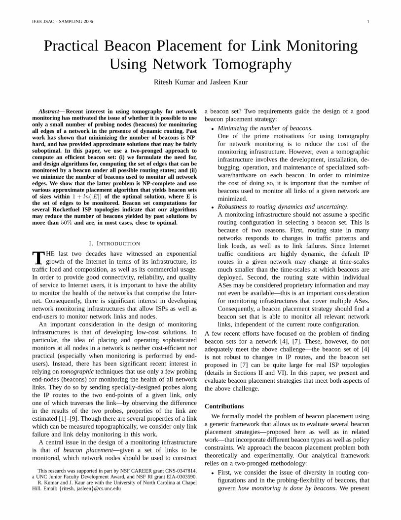
A
B C
Beacon A is "locally flexible"
MES = {AB, AC, BC}
A
B C
Beacon A is "simple"
MES = {AB, AC}
Fig. 1. Simple vs. Locally-flexible Beacons
to monitor a link in its MES, such a beacon—henceforthreferred to as a “simple” beacon—sends probes to theend-points of the link, along the default IP paths to thoseend-points. The authors demonstrate that the problem ofminimizing the size of the beacon set with such beacons isNP-hard, and provide a placement strategy that producesa beacon set no larger than1 + ln|E| times the optimalbeacon set. Unfortunately, since the authors assume thatall links within the routing tree of a beacon belong to itsMES, their strategy is not robust to changes in routingtrees and works only for networks with static routes.
• Locally-flexible Beacons:In [7], the authors consider beacons that have a greaterflexibility in selecting the paths taken by the probes.Specifically, the beacons—henceforth referred to as“locally-flexible” beacons—are capable of selecting thefirst link (outgoing link from beacon) on which a probeto any destination is transmitted. A probe can, therefore,be sent to a destination either along the current IP routeto the destination, or along one of the current IP routefrom any immediate neighbor to the same destination(see Figure 1).4 Furthermore, the authors do not assumestatic routing state and define the MES of a beacon toconsist of links that, irrespective of what current routesare, can always be monitored. The authors do not providea mechanism to compute such an MES for a beacon, butshow that even if these sets are known, the beacon setminimization problem is NP-hard. The authors insteadsuggest an alternative beacon-placement strategy which,unfortunately, can result in fairly large beacon sets forcurrent network topologies (see Section VI).
To summarize, existing beacon placement strategies areeither not robust to routing dynamics or are inefficient inminimizing the number of beacons.5
4The authors in [7] implicitly assume that the default IP route from anyneighbor to a given destination will not go through the beacon node. Thisassumption may get violated when a path through the beacon has a smallercost that any other physical path between a neighbor and the destination.
5An orthogonal problem of beacon placement for detectingmultiple linkfailures that occur simultaneously has been considered in [12]. In general,it is not possible to detect all cases of simultaneous link failures in a givennetwork. In [12], the authors restrict their attention to those simultaneous linkfailures that can be detected in the absence of any limitations on the number ofbeacons and probes. They then provide efficient algorithms for minimizing thenumber of beacons and probes needed for detecting these failures. Like [4],this work assumes “simple” beacons and uses the IP routing tree in the beaconset computation and, hence, is applicable only to networks with non-dynamicroutes. We believe that it is possible to use our formulations from this paperto extend the work in [12] to locally-flexible beacons, as well as to networkswith dynamic routing.
Our Approach
In this paper, we build on past work to address theselimitations by using a two-pronged approach:
1) Deterministic MES Computation: In order to achieverobustness to routing dynamics, for each candidate bea-con, we determine the set of edges—referred to as itsDeterministic MES (DMES)—that can be monitored byit underall possible routing configurations.
2) Beacon Set Minimization: In order to minimize in-frastructure cost, we address the problem of finding thesmallestbeacon set.
In the following two sections we present our abstractions andmethodologies for implementing the above for both simple andlocally-flexible beacons.
III. D ETERMINISTICALLY MONITORABLE EDGE SETS
The first key problem we need to solve is to find the setof edges that can be monitored by a beacon, independent ofthe routing configuration. This is formally captured in thefollowing definition.
Definition 1: An edge is said to bedeterministically moni-torableby a beacon if the beacon can monitor it under all pos-sible route configurations. TheDeterministically MonitorableEdge Set(DMES) of a beacon is the set of all deterministicallymonitorable edges associated with that beacon.
In what follows, we consider both simple and locally-flexible beacons and present algorithms for computing theirDMES. For clarity, we first establish an equivalence between“deterministically monitoring an edge” and the topologicalstructure of the network. Lemma 1 does that:
Lemma 1: If all possible (simple) physical paths from abeaconu to a nodey end in the same edgee, then u candeterministically monitor edgee.Proof: Since all possible simple physical paths fromu to yend ine, then the current network route fromu to y also endsin e.6 This implies that whenever a probe is sent fromu to yand it reachesy, the probe always passes through the edgee.If the other end-point ofe is x, any monitorable property ofe may be estimated regardless of the current routing state ofthe network, by sending probes fromu to each ofx andy.
The advantage of the above formulation is that it allowsus to ignore the network routing state, which isdynamicandderived from an exponentially large set of possible paths, anduse only thestatic topology of the network for computingthe DMES. This can be done by relying on graph-theoreticanalysis (such as depth-first search) for efficiently finding foreach potential beaconu, the set of edgese such that allphysical paths to one of the end-points ofe end in that edge.Lemma 1 ensures thatu can monitor such an edgee under allpossible route configurations.
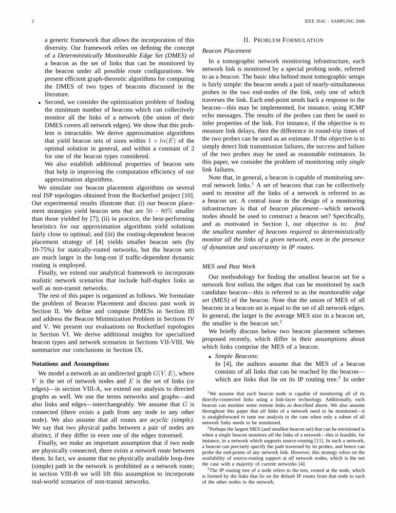
It is important to emphasize that there may be edges in agraph which may never qualify to become a DME using theformulation above. For example, in figure 2, the DMEs forall the nodes in a graph are the edges 1-2 and 5-6. To work
6This is because of our assumption that network routes are simple;therefore, the current route is also a member of the set of all simple physicalpaths fromu to y.
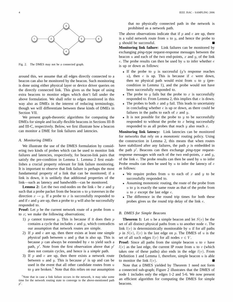
4 IEEE JSAC - SAMPLING 2006
1 2 5 6
3
4
Fig. 2. The DMES may not be a connected graph.
around this, we assume that all edges directly connected to abeacon can also be monitored by the beacon. Such monitoringis done using either physical layer or device driver queries onthe directly connected link. This gives us the hope of usingextra beacons to monitor edges which don’t fall under theabove formulation. We shall refer to edges monitored in thisway also as DMEs in the interest of reducing terminology,though we will differentiate between these kinds of DMEs inSection VII.
We present graph-theoretic algorithms for computing theDMEs for simple and locally-flexible beacons in Sections III-Band III-C, respectively. Below, we first illustrate how a beaconcan monitor a DME for link failures and latencies.
A. Monitoring DMEs
We illustrate the use of the DMES formulation by consid-ering two kinds of probes which can be used to monitor linkfailures and latencies, respectively, for beacon-link pairs thatsatisfy the pre-condition in Lemma 1. Lemma 2 first estab-lishes a crucial property relevant for link failure monitoring.It is important to observe that link failure is perhaps the mostfundamental property of a link that can be monitored; if alink is down, it is unlikely that additional properties of thelink—such as latency and bandwidth—can be monitored.
Lemma 2: Let the two end-nodes on the linke bex andysuch that a probe packet from the beaconu to y traverses in thedirectionx → y. If a probe tox is successfully responded toand ife andy are up, then a probe toy will also be successfullyresponded to.Proof: Let p be the current network route of a probe fromuto x; we make the following observations;
1) p cannot traversey. This is because if it does thenpcontains a cycle that includesx andy, which contradictsour assumption that network routes are simple.
2) If p and e are up, then there exists at least one simplephysicalpath betweenu and y that is also up. This isbecausep can always be extended bye to yield such apath, p′. Note from the first observation above thatp′
does not contain cycles, and hence is asimplepath.3) If p and e are up, then there exists a network route
betweenu and y. This is becausep′ is up and can beused in the event that all other candidate routes fromuto y are broken.7 Note that this relies on our assumption
7Note that in case a link failure occurs in the network, it may take sometime for the network routing state to converge to the above-mentioned pathp′.
that no physically connected path in the network isprohibited as a network path.
The above observations indicate that ifp and e are up, thereis a valid network route fromu to y, and hence the probe toy should be successful.Monitoring link failure: Link failures can be monitored byexchangingping-type request-response messages between thebeaconu and each of the two end-points,x andy, of the linke. The probe results can then be used byu to infer whethereis up or down as follows:
• If the probe to y is successful (y’s response reachesu), then e is up. This is because ife were down,then no physical path would exist fromu to y (pre-condition in Lemma 1), and the probe would not havebeen successfully responded to.
• The probe toy fails but the probe tox is successfullyresponded to. From Lemma 2, this implies thate is down.
• The probes to bothx andy fail. This leads to uncertaintyin concluding whethere is up or down, as there could befailures in the paths to each ofx andy.
• It is not possible for the probe toy to be successfullyresponded to without the probe tox being successfullyresponded to as all probes that reachy also reachx.
Monitoring link latency: Link latencies can be monitoredfor networks that rely on amonotonicrouting policy. Usingthe construction in Lemma 2, this means that when routeshave stabilized after any failures, the pathp is embedded inthe pathp′. Beacons can then exchangeping-type request-response messages with each of the two end-points,x andy,of the link e. The probe results can then be used byu to inferProbe results can then be used byu to infer the latency ofeas follows:
• We require probes fromu to each ofx and y to besuccessfully responded to.
• Assuming monotonic routing, the route of the probe fromu to y is exactly the same route as that of the probe fromu to x except the last edgee.
• The difference in the round trip times for both theseprobes gives us the round trip delay of the linke.
B. DMES for Simple Beacons
Theorem 1: Let u be a simple beacon and letS(v) be theset of all distinct physical paths fromu to another nodev. Thelink l(v) is deterministically monitorable byu if for all pathsp in S(v), l(v) is the last edge onp. The DMES ofu is theset of all such edgesl(v) for all nodesv ∈ V .Proof: Since all paths from the simple beaconu to v havel(v) as the last edge, the current IP route fromu to v (whichtakes one of these paths) also ends in the edgel(v). FromDefinition 1 and Lemma 1, therefore, simple beaconu is ableto monitor the linkl(v).
Note that a DMES yielded by Theorem 1 need not forma connected sub-graph; Figure 2 illustrates that the DMES ofnode 1 includes only the edges 1-2 and 5-6. We now presentan efficient algorithm for computing the DMES for simplebeacons.
RITESH KUMAR AND JASLEEN KAUR: PRACTICAL BEACON PLACEMENT FOR LINK MONITORING USING NETWORK TOMOGRAPHY 5
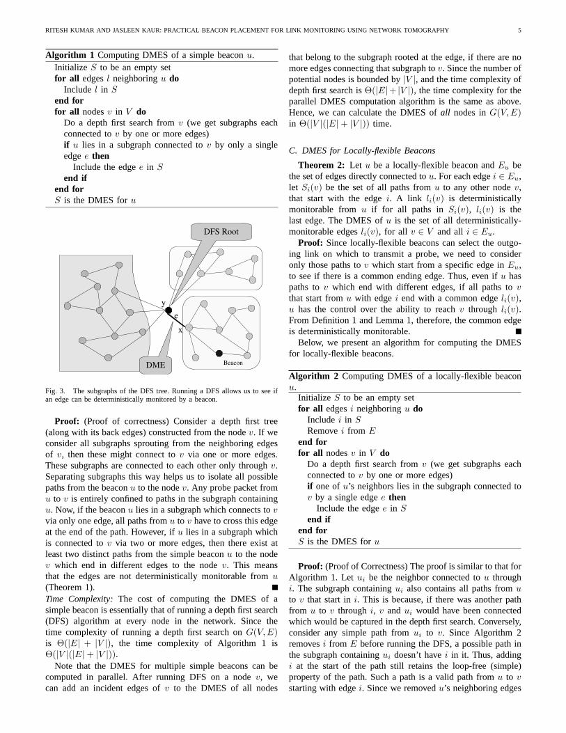
Algorithm 1 Computing DMES of a simple beaconu.Initialize S to be an empty setfor all edgesl neighboringu do
Include l in Send forfor all nodesv in V do
Do a depth first search fromv (we get subgraphs eachconnected tov by one or more edges)if u lies in a subgraph connected tov by only a singleedgee then
Include the edgee in Send if
end forS is the DMES foru
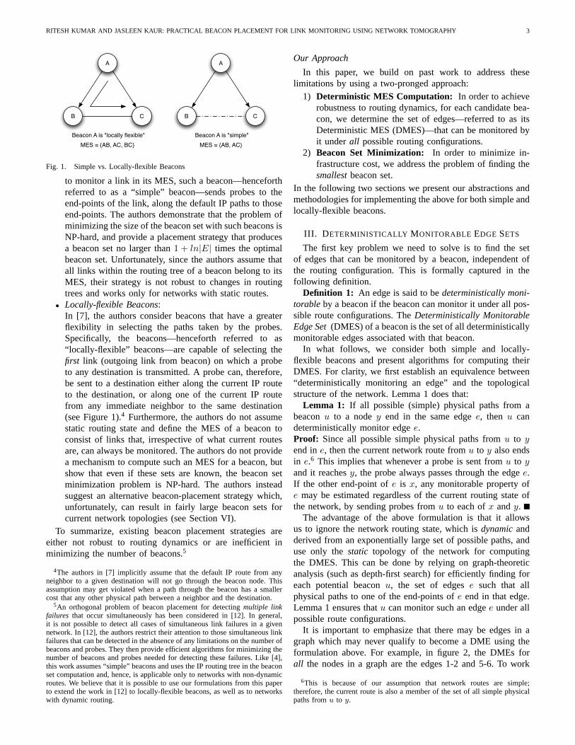
DFS Root
DME Beacon
y
x
e
Fig. 3. The subgraphs of the DFS tree. Running a DFS allows us to see ifan edge can be deterministically monitored by a beacon.
Proof: (Proof of correctness) Consider a depth first tree(along with its back edges) constructed from the nodev. If weconsider all subgraphs sprouting from the neighboring edgesof v, then these might connect tov via one or more edges.These subgraphs are connected to each other only throughv.Separating subgraphs this way helps us to isolate all possiblepaths from the beaconu to the nodev. Any probe packet fromu to v is entirely confined to paths in the subgraph containingu. Now, if the beaconu lies in a subgraph which connects tovvia only one edge, all paths fromu to v have to cross this edgeat the end of the path. However, ifu lies in a subgraph whichis connected tov via two or more edges, then there exist atleast two distinct paths from the simple beaconu to the nodev which end in different edges to the nodev. This meansthat the edges are not deterministically monitorable fromu(Theorem 1).Time Complexity:The cost of computing the DMES of asimple beacon is essentially that of running a depth first search(DFS) algorithm at every node in the network. Since thetime complexity of running a depth first search onG(V,E)is Θ(|E| + |V |), the time complexity of Algorithm 1 isΘ(|V |(|E|+ |V |)).
Note that the DMES for multiple simple beacons can becomputed in parallel. After running DFS on a nodev, wecan add an incident edges ofv to the DMES of all nodes
that belong to the subgraph rooted at the edge, if there are nomore edges connecting that subgraph tov. Since the number ofpotential nodes is bounded by|V |, and the time complexity ofdepth first search isΘ(|E|+ |V |), the time complexity for theparallel DMES computation algorithm is the same as above.Hence, we can calculate the DMES ofall nodes inG(V,E)in Θ(|V |(|E|+ |V |)) time.
C. DMES for Locally-flexible Beacons
Theorem 2: Let u be a locally-flexible beacon andEu bethe set of edges directly connected tou. For each edgei ∈ Eu,let Si(v) be the set of all paths fromu to any other nodev,that start with the edgei. A link li(v) is deterministicallymonitorable fromu if for all paths in Si(v), li(v) is thelast edge. The DMES ofu is the set of all deterministically-monitorable edgesli(v), for all v ∈ V and all i ∈ Eu.
Proof: Since locally-flexible beacons can select the outgo-ing link on which to transmit a probe, we need to consideronly those paths tov which start from a specific edge inEu,to see if there is a common ending edge. Thus, even ifu haspaths tov which end with different edges, if all paths tovthat start fromu with edgei end with a common edgeli(v),u has the control over the ability to reachv through li(v).From Definition 1 and Lemma 1, therefore, the common edgeis deterministically monitorable.
Below, we present an algorithm for computing the DMESfor locally-flexible beacons.
Algorithm 2 Computing DMES of a locally-flexible beaconu.
Initialize S to be an empty setfor all edgesi neighboringu do
Include i in SRemovei from E
end forfor all nodesv in V do
Do a depth first search fromv (we get subgraphs eachconnected tov by one or more edges)if one ofu’s neighbors lies in the subgraph connected tov by a single edgee then
Include the edgee in Send if
end forS is the DMES foru
Proof: (Proof of Correctness) The proof is similar to that forAlgorithm 1. Let ui be the neighbor connected tou throughi. The subgraph containingui also contains all paths fromuto v that start ini. This is because, if there was another pathfrom u to v throughi, v andui would have been connectedwhich would be captured in the depth first search. Conversely,consider any simple path fromui to v. Since Algorithm 2removesi from E before running the DFS, a possible path inthe subgraph containingui doesn’t havei in it. Thus, addingi at the start of the path still retains the loop-free (simple)property of the path. Such a path is a valid path fromu to vstarting with edgei. Since we removedu’s neighboring edges
6 IEEE JSAC - SAMPLING 2006
from E, one could argue that some paths might be missing.However, this cannot be true because no simple paths fromv to u would transitu in the middle of the path. Hence thesubgraphs obtained by removing the edges neighboringu arerepresentative of all paths fromu’s neighbors tov.Time Complexity:The cost of this algorithm is that of runninga depth first search on each node and for each depth firstsearch run checking if any of the neighbors of u are in a singlyconnected subgraph. Thus, if the degree ofu is k, the timecomplexity of the algorithm isΘ(|V |(|E|+ |V |+ k)). Sincek is bounded by|V |, the time complexity isΘ(|V |(|E| +|V |)). Note that, unlike simple beacons, DMES for locally-flexible beacons can not be computed in parallel for multiplenodes because for each locally-flexible beacon we customizethe graphG(V,E) (removal of neighboring edges) specificto the beacon before doing all the depth first searches. Thecomplexity of computing DMES forall nodes inG(V,E) is,therefore,Θ(|V |2(|E|+ |V |)).
IV. B EACON SET M INIMIZATION
The second key problem—of minimizing the beacon set fora network—is formally stated below:
Beacon Minimization Problem (BMP): Let Du be theDMES associated with a nodeu ∈ V . Then thebeacon-minimization problemis to find the smallest set of beacons,B ⊆ V , such that
⋃b∈B Db = E.
The Beacon Placement Problem is intractable for the beacontypes considered in this paper. We formally prove in sec-tion VII-A that BMP is NP-Complete for the case of simplebeacons. BMP has also been shown to be NP-complete forlocally-flexible beacons in [7]. Below we develop a correspon-dence between the general BMP (independent of beacon type)and Minimum Set Cover problem (MSCP)—this will let usapply well-known MSCP heuristics for addressing BMP.
Theorem 3: BMP is a special case of the Minimum SetCover problem.
Proof: MSCP [13] can be stated as follows. Consider a setS with elementse1, e2, ... . Now consider a group of arbitrarysubsets ofS; X1, X2, X3... such that
⋃i Xi = S. The Min
Set Cover problem is to find a collection ofXi’s (say setQ),such that
⋃Xi∈Q Xi = S and |Q| is the minimum.
To show that BMP is a special case of MSCP, considera graph G(V,E). Since every node can deterministicallymonitor at least its neighboring edges,
⋃v∈V Dv = E. Also,
∀v ∈ V : Dv ⊆ E. To solve BMP, we need to find thesmallestsubset,B ⊆ V , such that
⋃v∈B Dv = E; then B is the
required beacon set. Now consider a setB′ = {Dv : v ∈ B}.Note that|B′| = |B|. Also note the correspondence betweenMSCP and BMP given the associationsS → E,Xi → Dv
andQ → B′.MSCP is known to be NP-Complete [13], [14]. However,
MSCP has a pruning-based approximate solution—below, weadapt the pruning algorithm and use heuristics from theliterature [15] to establish approximate solutions with boundedoptimality for BMP.
It is straightforward to see that the algorithm returns a validbeacon set. This is because every edge that was eliminated
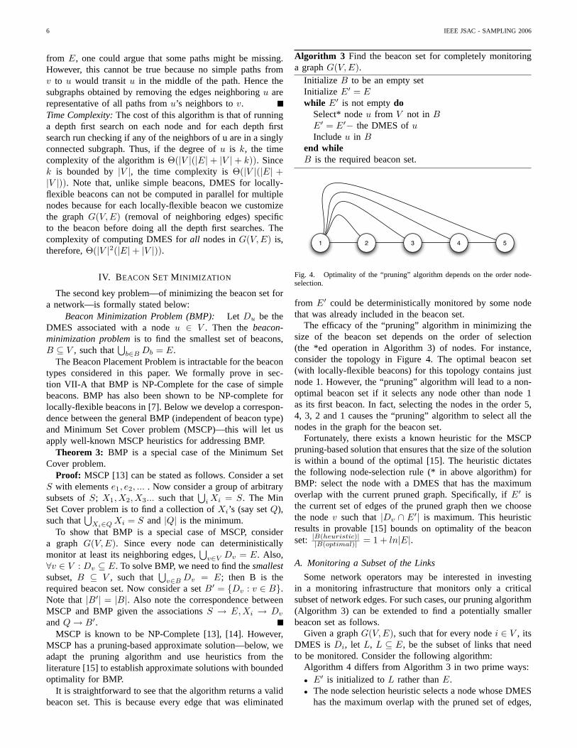
Algorithm 3 Find the beacon set for completely monitoringa graphG(V,E).
Initialize B to be an empty setInitialize E′ = Ewhile E′ is not emptydo
Select* nodeu from V not in BE′ = E′− the DMES ofuIncludeu in B
end whileB is the required beacon set.
1 2 3 4 5
Fig. 4. Optimality of the “pruning” algorithm depends on the order node-selection.
from E′ could be deterministically monitored by some nodethat was already included in the beacon set.
The efficacy of the “pruning” algorithm in minimizing thesize of the beacon set depends on the order of selection(the *ed operation in Algorithm 3) of nodes. For instance,consider the topology in Figure 4. The optimal beacon set(with locally-flexible beacons) for this topology contains justnode 1. However, the “pruning” algorithm will lead to a non-optimal beacon set if it selects any node other than node 1as its first beacon. In fact, selecting the nodes in the order 5,4, 3, 2 and 1 causes the “pruning” algorithm to select all thenodes in the graph for the beacon set.
Fortunately, there exists a known heuristic for the MSCPpruning-based solution that ensures that the size of the solutionis within a bound of the optimal [15]. The heuristic dictatesthe following node-selection rule (* in above algorithm) forBMP: select the node with a DMES that has the maximumoverlap with the current pruned graph. Specifically, ifE′ isthe current set of edges of the pruned graph then we choosethe nodev such that|Dv ∩ E′| is maximum. This heuristicresults in provable [15] bounds on optimality of the beaconset: |B(heuristic)|
|B(optimal)| = 1 + ln|E|.
A. Monitoring a Subset of the Links
Some network operators may be interested in investingin a monitoring infrastructure that monitors only a criticalsubset of network edges. For such cases, our pruning algorithm(Algorithm 3) can be extended to find a potentially smallerbeacon set as follows.
Given a graphG(V,E), such that for every nodei ∈ V , itsDMES is Di, let L, L ⊆ E, be the subset of links that needto be monitored. Consider the following algorithm:
Algorithm 4 differs from Algorithm 3 in two prime ways:• E′ is initialized toL rather thanE.• The node selection heuristic selects a node whose DMES
has the maximum overlap with the pruned set of edges,

RITESH KUMAR AND JASLEEN KAUR: PRACTICAL BEACON PLACEMENT FOR LINK MONITORING USING NETWORK TOMOGRAPHY 7
Algorithm 4 Find a beacon set to monitor the set of edgesLin the graphG(V,E).
Initialize B to be an empty setInitialize E′ = Lwhile E′ is not emptydo
Select* nodeu from V not in BE′ = E′− the DMES ofuIncludeu in B
end whileB is the required beacon set.
which is a subset ofL (still equivalent to “currentlypruned graph”).
Theorem 4: Algorithm 4 finds a beacon set for monitoringedges inL using no more thanΘ(1 + ln|L|) beacons.
Proof: Using the same terminology of beacons, DMES andlinks, consider a Min Set Cover problem as follows. Let theset of edgesE = L, the set of DMESs under consideration= {Di : Di ∩L 6= ∅}. By the node selection heuristic used inalgorithm 4, the algorithm reduces to the standard Min SetCover heuristic for the smaller instance of Min Set Coverproblem outlined above. Hence, the optimality of the solutionis bounded by the optimality bound for the smaller instanceof Min Set Cover problem which isΘ(1 + ln|L|).
V. H IGH ARITY NODES AND BEACON SETS
In [7], the authors introduced the concept of high aritynodes which was used in constructing a beacon set. In thissection, we show how the concept of node arity can be usefulin speeding-up the computation of a small beacon set, asformulated in Section IV. Below, we restate the definition ofnode arity from [7] in a slightly different manner.
Definition 2: (Node Arity) The arity of a node,u, withrespect to another node, v, is defined as the number of distinctpaths that exist between the two nodes such that each of thesepaths starts from a unique outgoing edge fromu. The arityof a nodeu is defined as the maximum of arities ofu withrespect all nodes of the graph.
Using the terminology of [7], we refer to a node as “higharity” if the node’s arity is more than one. Note that sinceG(V,E) is assumed to be connected, there is at least one pathfrom every node to every other node (assuming|V | > 1).Hence, the arity of a node is always greater than or equal toone. Also, since the maximum number of distinct paths (witha unique outgoing edge) fromu to v can not be more than thedegree ofu, the arity of a node is bounded by its degree.
Algorithm 7 in the Appendix gives an efficient way forfinding whether a node inG(V,E) is high arity or not. Ouralgorithm is based on the insight that if a nodev has arityone, all subgraphs generated in the depth-first search fromvwill be connected tov by a single edge.
A. Single Arity Networks
It is interesting to study the Beacon Placement Problem fora graphG(V,E) that contains only single arity nodes. We
show the optimal beacon set for such a graph is a singletonset, and can contain any one node of the graph.
Lemma 3: A graphG(V,E) with no high arity nodes is atree.
Proof: Since the graph is connected, the nodes present inthe graph have an arity of at least one. Since there are no higharity nodes in graph, the arity of all nodes is one. Supposethere is a cycle inG. Then, any two distinct nodes in the cyclehave separate paths to each other from their different outgoingedges. Thus, the nodes in the cycle are high arity, which isa contradiction. Hence, the graph cannot contain cycles. Thisimplies thatG(V,E) is a tree.
Theorem 5: A network with no high arity nodes can bemonitored by a single beacon on any node in the network.
Proof: From Lemma 3, we know that a network with nohigh arity nodes is a tree. Consider an arbitrary nodeu in thetree as a beacon; then the network graph can be consideredas a tree rooted atu. Since the graph is a tree, there is onlyone simple physical path available fromu to any other node.In particular, this implies that givenany network edgee, allphysical paths (in this graph, there is only one such path) fromu to one of the end-points ofe, end in the edgee. Thus,e is aDME of u. Thus, all edges of the graph belong to the DMESof u, and can be monitored by it.
B. High Arity Networks
We next show that using node arity analysis, the beaconsearch space in the pruning algorithms of Section IV canbe substantially reduced. Specifically, in Theorem 6 we showthat only high arity nodes need to be considered as potentialbeacons. Lemma 4 is used to prove the theorem.
Lemma 4: A graph which has at least one high arity nodecannot be completely monitored by a single simple or locally-flexible beacon placed on a single arity node.
Proof: Consider a graphG(V,E), which has a high aritynodex. Also consider a single beacon on a single arity nodeb. Sincex is a high arity node, there exists a nodey, to whichx has multiple paths with different outgoing edges fromxand multiple incoming edges toy. Thus,x andy are part ofa cycle.b cannot be on this cycle as otherwise it would behigh arity. Note thatb cannot deterministically monitor anyedges in this cycle. This is because for any edge in the cycle,b has multiple paths to one of its end-points, which end in adifferent edge. Hence,b cannot completely monitor the entiregraph.
Theorem 6: For a network with at least one high-aritynode, an optimal beacon set is a subset of the set of higharity nodes.
Proof: Let B be an optimal beacon set of graphG(V,E).Supposeb ∈ B is a single arity node. SinceB is optimal,removing b from B causes at least one edgee ∈ E to benot deterministically monitorable byB. Let x and y be thetwo nodes on either side ofe and, without loss of generality,assume thate is traversed when a probe packet is sent fromb toy (and hence not traversed when sent tox). Now consider adepth first search fromy. Consider the subgraphs sproutingfrom the edges adjacent toy. Since e is deterministically
8 IEEE JSAC - SAMPLING 2006
monitorable fromb, b lies in the subgraph,Fe, sprouting fromthe edgee. Also, Fe is connected toy by only e and noother edge (otherwise,e wouldn’t have been deterministicallymonitorable byb). Since,e was exclusively monitorable byonly b, there are no other beacons inFe.
Now consider the following two cases:• Fe has at least one high arity node.
Let h be a high arity node inFe. Sincee is the only edgeconnecting the subgraph to the rest of the graph,h mustbe high arity with respect to a node in the subgraph itself.Hence from Lemma 4,b cannot monitor the entire sub-graph. Also, no other beacon outsideFe can completelymonitorFe, as all paths from such beacons must traversee; just like b, such beacons can not deterministicallyguarantee the last edge in their paths to nodes in thecycle formed byh (Lemma 4). Sinceb should be able tomonitor the entire subgraph as it is the sole beacon in it,we have a contradiction. It follows that all nodes in thesubgraph must be single arity.
• Fe has only single arity nodes.If Fe contains only single arity nodes then all edges in thesubgraph can be monitored by a single beacon outside thesubgraph. This is becauseFe is a tree, and is reachableonly throughe from a beacon outsideFe. Any path froman outside beacon to any node inFe has a unique sub-path after crossinge. Hence, all edges withinFe can bemonitored by it. This implies thatb is a redundant beacon,and removingb from B doesn’t effect the monitorableedge coverage of the beacon setB. This contradicts thedefinition of B as an optimal beacon set.
Thus, there can not exist a single arity node inB. Hence,Bis a subset of the set of high arity nodes.
Theorem 6 lets us reduce the set of potential beacons usedin Algorithm 3 to the set of high arity nodes. This can leadto substantial computational savings. For instance, we showin Section VI (and Figure 6), that the fraction of single aritynodes in current ISP topologies can be quite high.
In [7] the authors have shown that the set of high arity nodesin a graph is a beacon set—though potentially a non-optimalset—when beacons are locally-flexible. We have strengthenedthis result by showing that the optimal beacon set isalwaysa subset of the set of high-arity nodes (even with simplebeacons). Hence, our pruning algorithm is potentially capableof finding smaller beacon sets for all topologies. In order toempirically evaluate the efficacy of our methodology, we nextcompute the beacon sets for a few real-world ISP topologies.
VI. EXPERIMENTAL RESULTS
In this section, we empirically evaluate the performance ofour beacon placement strategies. Specifically, we compare thesizes of beacons sets for several current ISP topologies, forwhich beacon sets are computed: (i) by the beacon placementsolution with locally-flexible beacons suggested in [7]; (ii)by our beacon placement algorithms for simple beacons; and(iii) by our algorithms for locally-flexible beacons. We alsostudy the overhead of incorporating dynamism in routing, bycomparing our solution to that obtained in [4], which appliesonly to statically-routed networks.
0
0.2
0.4
0.6
0.8
1
1 2 4 8 16 32 64 128
Frac
tion
of N
odes
Arity
AS: 1221AS: 1239AS: 1755AS: 2914AS: 3257AS: 3356AS: 3967AS: 4755AS: 6461AS: 7018
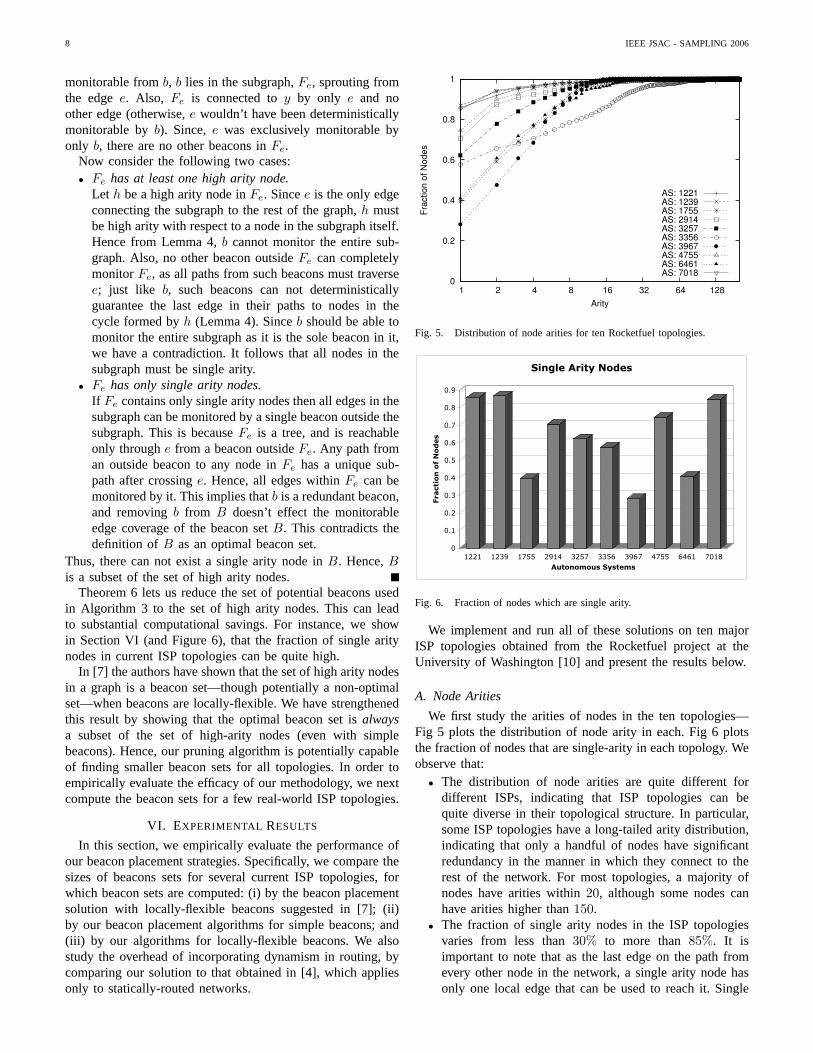
Fig. 5. Distribution of node arities for ten Rocketfuel topologies.
0
0.1
0.2
0.3
0.4
0.5
0.6
0.7
0.8
0.9
Fracti
on
of
No
des
1221 1239 1755 2914 3257 3356 3967 4755 6461 7018
Autonomous Systems
Single Arity Nodes
Fig. 6. Fraction of nodes which are single arity.
We implement and run all of these solutions on ten majorISP topologies obtained from the Rocketfuel project at theUniversity of Washington [10] and present the results below.
A. Node Arities
We first study the arities of nodes in the ten topologies—Fig 5 plots the distribution of node arity in each. Fig 6 plotsthe fraction of nodes that are single-arity in each topology. Weobserve that:
• The distribution of node arities are quite different fordifferent ISPs, indicating that ISP topologies can bequite diverse in their topological structure. In particular,some ISP topologies have a long-tailed arity distribution,indicating that only a handful of nodes have significantredundancy in the manner in which they connect to therest of the network. For most topologies, a majority ofnodes have arities within20, although some nodes canhave arities higher than150.
• The fraction of single arity nodes in the ISP topologiesvaries from less than30% to more than85%. It isimportant to note that as the last edge on the path fromevery other node in the network, a single arity node hasonly one local edge that can be used to reach it. Single
RITESH KUMAR AND JASLEEN KAUR: PRACTICAL BEACON PLACEMENT FOR LINK MONITORING USING NETWORK TOMOGRAPHY 9
0
200
400
600
800
1000
1200
1400
1600
1800
2000
Nu
mb
er o
f B
eaco
ns
1221 1239 1755 2914 3257 3356 3967 4755 6461 7018
Autonomous Systems
Comparison of Beacon Types
high arity nodes
Simple beacons
Locally flexible beacons
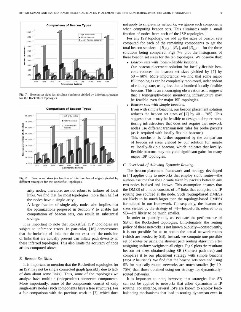
Fig. 7. Beacon set sizes (as absolute numbers) yielded by different strategiesfor the Rocketfuel topologies.
0.00%
10.00%
20.00%
30.00%
40.00%
50.00%
60.00%
70.00%
80.00%
Beaco
ns (
percen
tag
e o
f all n
od
es)
1221 1239 1755 2914 3257 3356 3967 4755 6461 7018
Autonomous Systems
Comparison of Beacon Types
high arity nodes
MSCP Heuristic
Locally flexible
beacons
Fig. 8. Beacon set sizes (as fraction of total number of edges) yielded bydifferent strategies for the Rocketfuel topologies.
arity nodes, therefore, are not robust to failures of locallinks. We find that for most topologies, more than half ofthe nodes have a single arity.A large fraction of single-arity nodes also implies thatthe optimizations proposed in Section V to enable fastcomputation of beacon sets, can result in substantialsavings.
It is important to note that Rocketfuel ISP topologies aresubject to inference errors. In particular, [16] demonstratesthat the inclusion of links that do not exist and the omissionof links that are actually present can inflate path diversity inthese inferred topologies. This also limits the accuracy of nodearities computed above.
B. Beacon Set Sizes
It is important to mention that the Rocketfuel topologies foran ISP may not be single connected graph (possibly due to lackof data about some links). Thus, some of the topologies weanalyze have multiple (independent) connected components.More importantly, some of the components consist of onlysingle-arity nodes (such components have a tree structure). Fora fair comparison with the previous work in [7], which does
not apply to single-arity networks, we ignore such componentswhen computing beacon sets. This eliminates only a smallfraction of nodes from each of the ISP topologies.
For any ISP topology, we add up the sizes of beacon setscomputed for each of the remaining components to get thetotal beacon set sizes—|BHA|, |BS |, and|BLF |—for the threesolutions being compared. Figs 7-8 plot the histograms ofthese beacon set sizes for the ten topologies. We observe that:
• Beacon sets with locally-flexible beacons.Our beacon placement solution for locally-flexible bea-cons reduces the beacon set sizes yielded by [7] by50 − 80%. More importantly, we find that some majorISP topologies can be completely monitored, independentof routing state, using less than a hundred locally-flexiblebeacons. This is an encouraging observation as it suggeststhat a tomography-based monitoring infrastructure maybe feasible even for major ISP topologies.
• Beacon sets with simple beacons.Even with simple beacons, our beacon placement solutionreduces the beacon set sizes of [7] by40 − 70%. Thissuggests that it may be feasible to design a simpler mon-itoring infrastructure that does not require that networknodes use different transmission rules for probe packets(as is required with locally-flexible beacons).This conclusion is further supported by the comparisonof beacon set sizes yielded by our solution for simplevs. locally-flexible beacons, which indicates that locally-flexible beacons may not yield significant gains for manymajor ISP topologies.
C. Overhead of Allowing Dynamic Routing
The beacon-placement framework and strategy developedin [4] applies only to networks that employstatic routes—theauthors assume that the IP route taken by packets between anytwo nodes is fixed and known. This assumption ensures thatthe DMES of a node consists ofall links that comprise the IProuting tree sourced at the node. Such routing-based DMESsare likely to be much larger than the topology-based DMESsformulated in our framework. Consequently, the beacon setsizes yielded by the strategy of [4]—henceforth, referred to asSB—are likely to be much smaller.
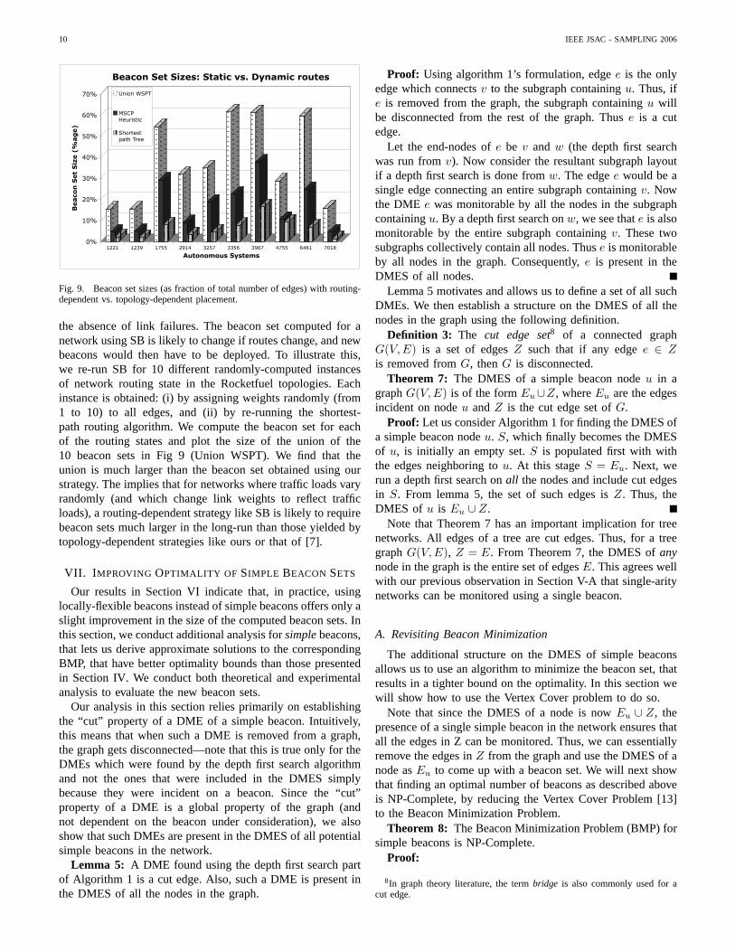
In order to quantify this, we evaluate the performance ofSB on the Rocketfuel topologies. Unfortunately, the routingpolicy of these networks is not known publicly—consequently,it is not possible for us to obtain the actual network routes(which are needed by SB). Instead, we compute one possibleset of routes by using the shortest path routing algorithm afterassigning uniform weights to all edges. Fig 9 plots the resultantbeacon set sizes obtained using SB (Shortest path tree) andcompares it to our placement strategy with simple beacons(MSCP heuristic). We find that the beacon sets obtained usingSB for statically-routed networks are much smaller (by 10-75%) than those obtained using our strategy for dynamically-routed networks.
It is important to note, however, that strategies like SBcan not be applied to networks that allow dynamism in IProuting. For instance, several ISPs are known to employ load-balancing mechanisms that lead to routing dynamism even in
10 IEEE JSAC - SAMPLING 2006
0%
10%
20%
30%
40%
50%
60%
70%
Beaco
n S
et
Siz
e (
%ag
e)
1221 1239 1755 2914 3257 3356 3967 4755 6461 7018
Autonomous Systems
Beacon Set Sizes: Static vs. Dynamic routes
Union WSPT
MSCP
Heuristic
Shortest
path Tree
Fig. 9. Beacon set sizes (as fraction of total number of edges) with routing-dependent vs. topology-dependent placement.
the absence of link failures. The beacon set computed for anetwork using SB is likely to change if routes change, and newbeacons would then have to be deployed. To illustrate this,we re-run SB for 10 different randomly-computed instancesof network routing state in the Rocketfuel topologies. Eachinstance is obtained: (i) by assigning weights randomly (from1 to 10) to all edges, and (ii) by re-running the shortest-path routing algorithm. We compute the beacon set for eachof the routing states and plot the size of the union of the10 beacon sets in Fig 9 (Union WSPT). We find that theunion is much larger than the beacon set obtained using ourstrategy. The implies that for networks where traffic loads varyrandomly (and which change link weights to reflect trafficloads), a routing-dependent strategy like SB is likely to requirebeacon sets much larger in the long-run than those yielded bytopology-dependent strategies like ours or that of [7].
VII. I MPROVING OPTIMALITY OF SIMPLE BEACON SETS
Our results in Section VI indicate that, in practice, usinglocally-flexible beacons instead of simple beacons offers only aslight improvement in the size of the computed beacon sets. Inthis section, we conduct additional analysis forsimplebeacons,that lets us derive approximate solutions to the correspondingBMP, that have better optimality bounds than those presentedin Section IV. We conduct both theoretical and experimentalanalysis to evaluate the new beacon sets.
Our analysis in this section relies primarily on establishingthe “cut” property of a DME of a simple beacon. Intuitively,this means that when such a DME is removed from a graph,the graph gets disconnected—note that this is true only for theDMEs which were found by the depth first search algorithmand not the ones that were included in the DMES simplybecause they were incident on a beacon. Since the “cut”property of a DME is a global property of the graph (andnot dependent on the beacon under consideration), we alsoshow that such DMEs are present in the DMES of all potentialsimple beacons in the network.
Lemma 5: A DME found using the depth first search partof Algorithm 1 is a cut edge. Also, such a DME is present inthe DMES of all the nodes in the graph.
Proof: Using algorithm 1’s formulation, edgee is the onlyedge which connectsv to the subgraph containingu. Thus, ife is removed from the graph, the subgraph containingu willbe disconnected from the rest of the graph. Thuse is a cutedge.
Let the end-nodes ofe be v and w (the depth first searchwas run fromv). Now consider the resultant subgraph layoutif a depth first search is done fromw. The edgee would be asingle edge connecting an entire subgraph containingv. Nowthe DME e was monitorable by all the nodes in the subgraphcontainingu. By a depth first search onw, we see thate is alsomonitorable by the entire subgraph containingv. These twosubgraphs collectively contain all nodes. Thuse is monitorableby all nodes in the graph. Consequently,e is present in theDMES of all nodes.
Lemma 5 motivates and allows us to define a set of all suchDMEs. We then establish a structure on the DMES of all thenodes in the graph using the following definition.
Definition 3: The cut edge set8 of a connected graphG(V,E) is a set of edgesZ such that if any edgee ∈ Zis removed fromG, thenG is disconnected.
Theorem 7: The DMES of a simple beacon nodeu in agraphG(V,E) is of the formEu∪Z, whereEu are the edgesincident on nodeu andZ is the cut edge set ofG.
Proof: Let us consider Algorithm 1 for finding the DMES ofa simple beacon nodeu. S, which finally becomes the DMESof u, is initially an empty set.S is populated first with withthe edges neighboring tou. At this stageS = Eu. Next, werun a depth first search onall the nodes and include cut edgesin S. From lemma 5, the set of such edges isZ. Thus, theDMES of u is Eu ∪ Z.
Note that Theorem 7 has an important implication for treenetworks. All edges of a tree are cut edges. Thus, for a treegraphG(V,E), Z = E. From Theorem 7, the DMES ofanynode in the graph is the entire set of edgesE. This agrees wellwith our previous observation in Section V-A that single-aritynetworks can be monitored using a single beacon.
A. Revisiting Beacon Minimization
The additional structure on the DMES of simple beaconsallows us to use an algorithm to minimize the beacon set, thatresults in a tighter bound on the optimality. In this section wewill show how to use the Vertex Cover problem to do so.
Note that since the DMES of a node is nowEu ∪ Z, thepresence of a single simple beacon in the network ensures thatall the edges in Z can be monitored. Thus, we can essentiallyremove the edges inZ from the graph and use the DMES of anode asEu to come up with a beacon set. We will next showthat finding an optimal number of beacons as described aboveis NP-Complete, by reducing the Vertex Cover Problem [13]to the Beacon Minimization Problem.
Theorem 8: The Beacon Minimization Problem (BMP) forsimple beacons is NP-Complete.
Proof:
8In graph theory literature, the termbridge is also commonly used for acut edge.
RITESH KUMAR AND JASLEEN KAUR: PRACTICAL BEACON PLACEMENT FOR LINK MONITORING USING NETWORK TOMOGRAPHY 11
BMP is in NP: We have shown how to obtain the DMESfor all the nodes in the beacon set in polynomial time. Hencetaking a union of the DMESs and comparing it with the set ofall edges allows us to verify in polynomial time if the solutionis correct. This proves that the BMP is in NP.
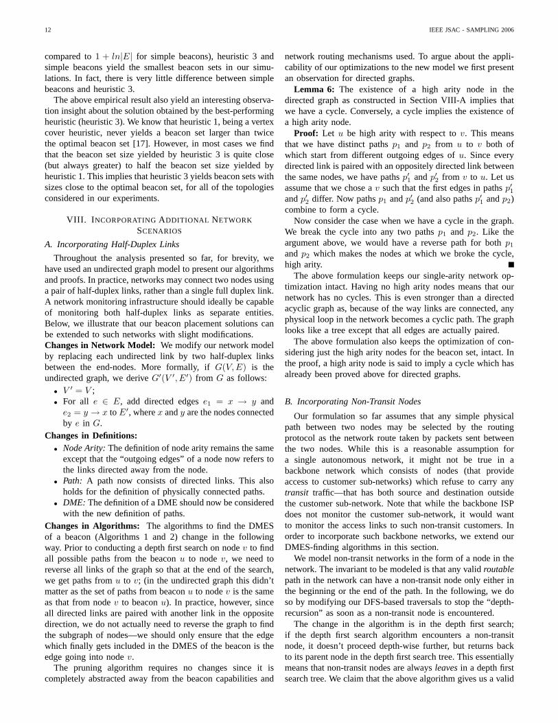
Reduction from Vertex Cover:Consider an instance ofa vertex cover problem with a graphG′(V ′, E′). In general,this graph may have one or more cut edges. We construct aninstance of BMP from this setup as follows:• For every cut edgee (with end nodesx andy) in E′, add a
nodene and edgespe andqe so thate, pe andqe form a trianglewith pe and qe incident onne. Now, the resultant graph (sayG′′(V ′′, E′′)) doesn’t have any cut edges, as removing any ofthe edgese still keepsG′′ connected.• Now, consider the Beacon Minimization Problem on graph
G′′. SinceG′′ has no cut edges, the DMES of a nodeu in G′′
reduces toE′′u (the edges incident onu).
ne
qepe
ex y
• Now, consider a solution to theBMP on G′′. We have a set of nodesB such that all the edges are “covered”(⋃
u∈B E′′u = E′′). Note that the sense
of “covered” used here is exactly thesame as the sense of “vertex covered”in the Vertex Cover problem.
To get a solution for the VertexCover problem from a solution to the BMP, consider any ofthe triangles (e, pe, qe) that were introduced above.• To cover all the three edges, we need exactly two nodes
(betweenx, y and ne). Thus, two of these three nodes arepresent inB. If ne is present inB then it covers bothpe
and qe. Hence, removingne, pe and qe from G′′ (and ne
from B) ensures that the resultant graph can still be optimally“covered” by B. This is becausene was not covering anyother edge other thanpe andqe.• If ne is absent fromB then we first check if puttingne
in B and removing eitherx or y from B leaves any of theedges in the graph uncovered. If it doesn’t then we have twooptimal solutions to the beacon placement problem and weuse the argument given above. However, if the transformationdoesn’t give us another optimal solution then it means thatxandy are single handedly “covering” more edges then justpe
and qe. Thus removingne, pe and qe from G′′ still ensuresthat all the edges are covered optimally.• We repeat this for all thene, pe andqe that we introduced
to get a solution to the Vertex Cover problem onG′(V ′, E′).Since Vertex Cover is NP-Complete [17] the above implies
that BMP is also NP-Complete.We use a known approximate solution to the Vertex Cover
problem for deriving the following algorithm which yields anapproximately-optimal beacon set.
Algorithm 5 has a known optimality bound of a constant2 [17]). Note that this constant bound of 2 does not dependon the edge selection heuristic used (select*) in the abovealgorithm. Below, we enumerate three heuristics that we studynext.
1) Heuristic 1 (random):We select the edges in the orderthey appear in the Rocketfuel data. The Rocketfuel datais arranged in an adjacency list format with node ids
Algorithm 5 Compute a beacon set using the approximateVertex Cover algorithm.
Initialize B to be an empty setRemove the edges inZ from G to getG′
while G′ contains edgesdoSelect* an edge fromG′
Include both its end nodes inBRemove the edge, its two end nodes and their edges fromG′
end whileB is the required Beacon Set.
0%
10%
20%
30%
40%
50%
60%
70%
Beaco
n S
et
Siz
e (
%ag
e)
1221 1239 1755 2914 3257 3356 3967 4755 6461 7018
Autonomous Systems
Beacon Set Size Percentages
Vertex
Cover 1
Vertex
Cover 2
Vertex
Cover 3
MSCP
Heuristic
Fig. 10. Comparison of vertex cover heuristics forsimplebeacons
followed by the list of nodes adjacent to it. There isno specific ordering to these nodes besides that they aresorted based on their identifier value. In this heuristic,we select the edge formed by the first node listed in thepruned graph and the first node in the adjacency list ofthe node. This essentially means that the edge selectioncriteria is fairly random.
2) Heuristic 2 (degree-order):We sort the nodes of thegraph according to their degrees; we also sort the nodesin the adjacency list (of a particular node) according totheir degrees. We then use heuristic 1 on this prepro-cessed graph representation.
3) Heuristic 3 (MSCP-adapted):This heuristic maps di-rectly to the Min Set Cover heuristic adopted in sec-tion IV. However, this is not an edge-selection heuristic,but a node-selection heuristic. We calculate the degreeof all the nodes in the graph and select the one with thehighest degree. We then include this node in our beaconset, remove this node (and its edges) from the graph andrecalculate degrees.
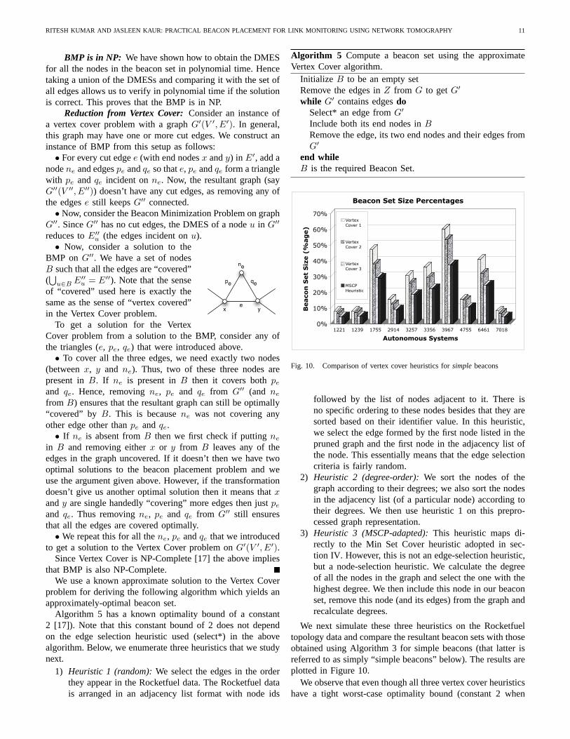
We next simulate these three heuristics on the Rocketfueltopology data and compare the resultant beacon sets with thoseobtained using Algorithm 3 for simple beacons (that latter isreferred to as simply “simple beacons” below). The results areplotted in Figure 10.
We observe that even though all three vertex cover heuristicshave a tight worst-case optimality bound (constant 2 when
12 IEEE JSAC - SAMPLING 2006
compared to1 + ln|E| for simple beacons), heuristic 3 andsimple beacons yield the smallest beacon sets in our simu-lations. In fact, there is very little difference between simplebeacons and heuristic 3.
The above empirical result also yield an interesting observa-tion insight about the solution obtained by the best-performingheuristic (heuristic 3). We know that heuristic 1, being a vertexcover heuristic, never yields a beacon set larger than twicethe optimal beacon set [17]. However, in most cases we findthat the beacon set size yielded by heuristic 3 is quite close(but always greater) to half the beacon set size yielded byheuristic 1. This implies that heuristic 3 yields beacon sets withsizes close to the optimal beacon set, for all of the topologiesconsidered in our experiments.
VIII. I NCORPORATINGADDITIONAL NETWORK
SCENARIOS
A. Incorporating Half-Duplex Links
Throughout the analysis presented so far, for brevity, wehave used an undirected graph model to present our algorithmsand proofs. In practice, networks may connect two nodes usinga pair of half-duplex links, rather than a single full duplex link.A network monitoring infrastructure should ideally be capableof monitoring both half-duplex links as separate entities.Below, we illustrate that our beacon placement solutions canbe extended to such networks with slight modifications.Changes in Network Model: We modify our network modelby replacing each undirected link by two half-duplex linksbetween the end-nodes. More formally, ifG(V,E) is theundirected graph, we deriveG′(V ′, E′) from G as follows:
• V ′ = V ;• For all e ∈ E, add directed edgese1 = x → y and
e2 = y → x to E′, wherex andy are the nodes connectedby e in G.
Changes in Definitions:• Node Arity:The definition of node arity remains the same
except that the “outgoing edges” of a node now refers tothe links directed away from the node.
• Path: A path now consists of directed links. This alsoholds for the definition of physically connected paths.
• DME: The definition of a DME should now be consideredwith the new definition of paths.
Changes in Algorithms: The algorithms to find the DMESof a beacon (Algorithms 1 and 2) change in the followingway. Prior to conducting a depth first search on nodev to findall possible paths from the beaconu to nodev, we need toreverse all links of the graph so that at the end of the search,we get paths fromu to v; (in the undirected graph this didn’tmatter as the set of paths from beaconu to nodev is the sameas that from nodev to beaconu). In practice, however, sinceall directed links are paired with another link in the oppositedirection, we do not actually need to reverse the graph to findthe subgraph of nodes—we should only ensure that the edgewhich finally gets included in the DMES of the beacon is theedge going into nodev.
The pruning algorithm requires no changes since it iscompletely abstracted away from the beacon capabilities and
network routing mechanisms used. To argue about the appli-cability of our optimizations to the new model we first presentan observation for directed graphs.
Lemma 6: The existence of a high arity node in thedirected graph as constructed in Section VIII-A implies thatwe have a cycle. Conversely, a cycle implies the existence ofa high arity node.
Proof: Let u be high arity with respect tov. This meansthat we have distinct pathsp1 and p2 from u to v both ofwhich start from different outgoing edges ofu. Since everydirected link is paired with an oppositely directed link betweenthe same nodes, we have pathsp′1 andp′2 from v to u. Let usassume that we chose av such that the first edges in pathsp′1andp′2 differ. Now pathsp1 andp′2 (and also pathsp′1 andp2)combine to form a cycle.
Now consider the case when we have a cycle in the graph.We break the cycle into any two pathsp1 and p2. Like theargument above, we would have a reverse path for bothp1
andp2 which makes the nodes at which we broke the cycle,high arity.
The above formulation keeps our single-arity network op-timization intact. Having no high arity nodes means that ournetwork has no cycles. This is even stronger than a directedacyclic graph as, because of the way links are connected, anyphysical loop in the network becomes a cyclic path. The graphlooks like a tree except that all edges are actually paired.
The above formulation also keeps the optimization of con-sidering just the high arity nodes for the beacon set, intact. Inthe proof, a high arity node is said to imply a cycle which hasalready been proved above for directed graphs.
B. Incorporating Non-Transit Nodes
Our formulation so far assumes that any simple physicalpath between two nodes may be selected by the routingprotocol as the network route taken by packets sent betweenthe two nodes. While this is a reasonable assumption fora single autonomous network, it might not be true in abackbone network which consists of nodes (that provideaccess to customer sub-networks) which refuse to carry anytransit traffic—that has both source and destination outsidethe customer sub-network. Note that while the backbone ISPdoes not monitor the customer sub-network, it would wantto monitor the access links to such non-transit customers. Inorder to incorporate such backbone networks, we extend ourDMES-finding algorithms in this section.
We model non-transit networks in the form of a node in thenetwork. The invariant to be modeled is that any validroutablepath in the network can have a non-transit node only either inthe beginning or the end of the path. In the following, we doso by modifying our DFS-based traversals to stop the “depth-recursion” as soon as a non-transit node is encountered.
The change in the algorithm is in the depth first search;if the depth first search algorithm encounters a non-transitnode, it doesn’t proceed depth-wise further, but returns backto its parent node in the depth first search tree. This essentiallymeans that non-transit nodes are alwaysleavesin a depth firstsearch tree. We claim that the above algorithm gives us a valid
RITESH KUMAR AND JASLEEN KAUR: PRACTICAL BEACON PLACEMENT FOR LINK MONITORING USING NETWORK TOMOGRAPHY 13
Algorithm 6 Find the DMES of a simple beaconu in a graphG(V,E) containing non-transit nodes.Consider a modification of algorithm 1.
Initialize S to be an empty setfor all edgesl neighboringu do
Include l in Send forfor all nodesv in V do
Do a modified depth first search fromv such that onvisiting a non-transit node we don’t proceed furtherrecursively but we retract to the parent node in the DFStree; we don’t stop at the root node if the root is a non-transit node. (we get a set of subgraphs each connectedto v by one or more edges)if u lies in a subgraph connected tov by only a singleedgee then
Include the edge in Send if
end forS is the DMES ofu
optimal DMES for the beaconu in G(V,E) containing non-transit nodes.
Proof: (Proof of correctness) Since non-transit nodes don’tallow transit traffic, any valid path inG(V,E) now can containa non-transit node only at the start or the end. Consider a graphG′ which is the same asG(V,E) minus all non-transit nodesand its neighboring edges. Note thatG′ might not be connectedeven if G is. Let us denote the set of paths between the nodepair (x, y) by the symbolPx,y. Because of the characteristicof the non-transit nodes, the set of paths for a node pair(x, y)in G(V,E) can be described as;
• if x andy are not non-transit nodes, then the set of pathsPx,y remains the same in bothG andG′.
• if x is a non-transit node, then the set of pathsPx,y inG is equal to
⋃x′ [(x, x′) + Px′,y in G′] wherex′ is not
a non-transit node and adjacent tox.• if x andy are non-transit nodes, then the set of pathsPx,y
in G is equal to⋃
x′,y′ [(x, x′) + Px′,y′ in G′ + (y′, y)]wherex′ is a normal node and adjacent tox andy′ is anormal node and adjacent toy.
We have to prove that if and only if two nodesx, y inG(V,E) are connected by a network route, then there exists apath in the (modified) depth first tree which connects the twonodes. We consider the following cases:
• Case 1: If x and y are normal nodes, then from theabove, existence of a non-emptyPx,y in G′ implies a non-emptyPx,y in G. Also, any path inPx,y doesn’t containnon-transit nodes. Hence, our modified depth first searchalgorithm connects these two nodes.Conversely, ifPx,y in G′ is empty, then (because initiallyG was connected), we can conclude that all paths inPx,y
had non-transit nodes in the middle. Our modified depthfirst search algorithm will not connectx and y as onall paths it finds a non-transit node on and halt furtherdepth-wise graph search from that point onward.
• Case 2:If any of x and/ory are non-transit nodes, thenderivation ofPx,y in G from Px′,y′ in G′ is given above.This enumerates all paths that can exist betweenx andy in G assuming these are the only non-transit nodespresent in the network. Without loss of generality, let usassume thatx is a non-transit node;y may or may notbe a non-transit node. IfPx,y is non-empty inG, thenthere exists a non-emptyPx′,y′ as described above. Anon-emptyPx′,y′ implies thatx′ and y′ are connectedby our modified depth first search algorithm inG. Thisfollows directly from Case 1. Since our modified depthfirst search algorithm connectsx to x′ (depth first startingfrom root doesn’t stop at root because the root is a non-transit node), it also connectsx to y′. Also, since ourmodified depth first search algorithm connects any non-transit node to a normal neighbor node, it joinsy′ andy.Thus our modified depth first search algorithm connectsx andy.Conversely, ifPx,y is empty inG, it means that for allneighbors ofx (and possiblyy if y is a non-transit node),Px′,y′ is empty. From Case 1, we can conclude that ourmodified depth first search algorithm doesn’t connect anyof thosex′ and y′. Thus,x and y are not connected byour modified depth first search algorithm.
• Case 3:A trivial border case which is not easily evidentfrom the above is about two non-transit nodesx andy, directly connected. Our modified depth first searchalgorithm correctly connects them.
Using the above connectivity proof, along with the proof ofcorrectness of Algorithm 1, we establish the correctness ofAlgorithm 6. Though the above is shown only for simplebeacons, the same connectivity argument also holds for theDMES algorithm for locally-flexible beacons.
C. Robustness tok beacon failures
A tomographic monitoring infrastructure should ideally berobust to beacon failures; in particular, there should be nolinks in the network that can be monitored by only a singlebeacon. To achieve robustness to beacon failures, therefore,a monitoring infrastructure may wish to instantiate additional(possibly redundant) beacons in the network. A beacon set issaid to be robust tok beacon failures if any subset of thebeacon set containingk less beacons is able to monitor thecomplete network.
In [4], the authors have presented a technique for computingsuch robust beacon sets, using an extended version of the MinSet Cover problem. We believe their solution is general enoughto be applicable to the beacon-placement framework presentedin this paper. A detailed treatment of this scenario is, however,beyond the scope of this paper.
IX. CONCLUDING REMARKS
In this paper, we have presented a generic framework foraddressing the problem of beacon placement for networkmonitoring using tomography, efficiently and under a genericset of policy constraints. Our framework incorporates routingdynamism and monitoring policy constraints by defining the

14 IEEE JSAC - SAMPLING 2006
generic concept of Deterministically Monitorable Edge Sets,and then using the DMESs to find beacon sets that are within abounded-range of the optimal size for monitoring a given set ofnetwork edges. We extend our basic framework to incorporatenetworks consisting of half-duplex links as well as non-transitsub-networks.
We supplement our theoretical analysis with empirical re-sults obtained from running beacon placement strategies onRocketfuel versions of real-world ISP topologies. We findthat our algorithms perform significantly better than previoustechniques and reduce the beacon set size by about 50 to80%. We also find that the best-performing heuristic used forplacement of “simple” beacons, yields beacon sets fairly closeto optimal.
Acknowledgments: The authors thanks the anonymousJSAC reviewers for their valuable feedback and suggestions.
REFERENCES
[1] CAIDA, “Skitter,” http://www.caida.org/tools/ measurement/skitter.[2] M. Coates, A. Hero, R. Nowak, and B. Yu, “Internet tomography,”IEEE
Signal Processing Magazine, May 2002.[3] K. Claffy, T. Monk, and D. McRobb, “Internet tomography,”Nature,
January 1999.[4] Y. Bejerano and R. Rastogi, “Robust monitoring of link delays and faults
in ip networks,” in Proceedings of the 2003 ACM INFOCOM, April2003. [Online]. Available: citeseer.ist.psu.edu/bejerano03robust.html
[5] N. Duffield and F. L. Presti, “Multicast inference of packet delayvariance at interior network links,” inINFOCOM, vol. 3, 2000, pp.1351–1360.
[6] N. Duffield, J. Horowitz, F. L. Presti, and D. Towsley, “Network delaytomography from end-to-end unicast measurements,”Lecture Notes inComputer Science, vol. 2170, pp. 576–595, 2001.
[7] J. Horton and A. Lopez-Ortiz, “On the number of distributed measure-ment points for network tomography,” inProceedings of the ACM SIG-COMM Internet Measurement Conference (extended abstract), October2003, pp. 204–209.
[8] R. Kumar and J. Kaur, “Efficient beacon placement for network to-mography,”(extended abstract) in Proceedings of Internet MeasurementConference, October 2004.
[9] P. Barford, A. Bestavros, J. Byers, and M. Crovella, “On the marginalutility of network topology measurements,” inProceedings of the 1stACM SIGCOMM Workshop on Internet Measurement, November 2001,pp. 5 – 17.
[10] N. Spring, R. Mahajan, and D. Wetherall, “Measuring isp topologieswith rocketfuel,” in Proceedings of ACM SIGCOMM, vol. 32, August2002. [Online]. Available: citeseer.ist.psu.edu/spring02measuring.html
[11] P. et. al., “Rfc 791: Internet protocol,”Request for Comments, pp. 17–18,1999.
[12] H. Nguyen and P. Thiran, “Active measurement for multiple linkfailures diagnosis in ip networks,” inProceedings of Passive and ActiveMeasurement Workshop (PAM), April 2004.
[13] T. Cormen, C. Stein, R. Rivest, and C. Leiserson,Introduction toAlgorithms. McGraw-Hill Higher Education, 2001.
[14] M. Garey and D. Johnson,Computers and Intractability: A Guide to theTheory of NP-Completeness. W. H. Freeman & Co., 1979.
[15] T. Cormen, C. Leiserson, and R. Rivest, “Theorem 35.4, minimum setcover,” Introduction to Algorithms, Second Edition, 2001.
[16] R. Teixeira, K. Marzullo, S. Savage, and G. Voelker, “In search ofpath diversity in isp networks,” inProceedings of the ACM SIGCOMMInternet Measurement Conference, October 2003.
[17] T. Cormen, C. Leiserson, and R. Rivest, “Theorem 35.1, vertex cover,”Introduction to Algorithms, Second Edition, 2001.
APPENDIX
Proof: (Proof of Correctness) Consider the case whenu ishigh arity. Then there exists a node (sayv) to which thereare more than one paths fromu with different outgoing edgesfrom u. In a depth first search fromu, one of these edges will
Algorithm 7 Finding out if a node,u in G(V,E) is high arityor not.
Do a depth first search fromu;if there is a back edge tou from any other nodethen
declareu high arityelse
declareu single arityend if
be selected first for traversal. In the depth first search run,consider that we are on the first edge fromu which has a pathto v, with an alternating path to the same nodev as definedabove. Because of the alternating path, there exists a cyclewith nodesu and v on it. Since the edge on the alternatingpath outgoing fromu is not yet traversed, it will become aback edge and will be detected as outlined in the algorithm.
Now consider that nodeu is not a high arity node. Alsoassume that we detect a back edge in the way outlined inthe algorithm. Since the back edge was to nodeu itself, itmeans that nodeu is part of a cycle with two outgoing edgesparticipating in the cycle. Thus, there is at least one node inthe network (from the same cycle) which has two paths toueach path having a different outgoing edge fromu. This meansthat u is a high arity node. This is a contradiction. Hence ifu is an arity one node then one cannot detect a back edge asdescribed in the algorithm.
Time Complexity:The complexity of depth first search isΘ(|E| + |V |). Detecting a back edge involves going throughall the neighbors ofu. If the degree ofu is k, then the costfor checking for a back edge isΘ(k). Sincek is bounded by|E|, the time complexity of our algorithm isΘ(|E|+ |V |).
Ritesh Kumar is a Graduate Student in the Depart-ment of Computer Science at the University of NorthCarolina at Chapel Hill. His research interests lie incomputer networks, and especially in the design ofend-to-end transport protocols.
Ritesh received his B.Tech. in Computer Scienceand Engineering from the Indian Institute of Tech-nology, Kanpur, in 2003.
Jasleen Kaur is an Assistant Professor in the De-partment of Computer Science at the University ofNorth Carolina at Chapel Hill. Her research interestslie in the design and evaluation of networks andoperating systems. Jasleen is a recipient of the NSFCAREER Award, 2004, and the UNC Junior FacultyDevelopment Award, 2004.
Jasleen received her B.Tech. in Computer Sci-ence and Engineering from the Indian Institute ofTechnology, Kanpur, in 1997, where she was alsoawarded the Motorola Student of the Year Gold
Medal. She earned an M.S. and Ph.D. in Computer Sciences from theUniversity of Texas at Austin in 1999 and 2002, respectively. She is a recipientof the J.C.Browne Graduate Fellowship and the M.C.D. Fellowship from theUniversity of Texas at Austin.