ie 361 module 6
TRANSCRIPT

IE 361 Module 6Gauge R&R Studies Part 2: Two-Way ANOVA and Corresponding
Estimates for R&R Studies
Reading: Section 2.2 Statistical Quality Assurance for Engineers(Section 2.4 of Revised SQAME )
Prof. Steve Vardeman and Prof. Max Morris
Iowa State University
Vardeman and Morris (Iowa State University) IE 361 Module 6 1 / 21
ANOVA and R&R Analysis
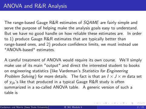
The range-based Gauge R&R estimates of SQAME are fairly simple andserve the purpose of helping make the analysis goals easy to understand.But we have no good handle on how reliable these estimates are. In orderto 1) produce Gauge R&R estimates that are typically better thanrange-based ones, and 2) produce confidence limits, we must instead use"ANOVA-based" estimates.
A careful treatment of ANOVA would require its own course. We’ll simplymake use of its main "output" and direct the interested student to bookson engineering statistics (like Vardeman’s Statistics for EngineeringProblem Solving) for more details. The fact is that an I × J ×m data setof yijk’s like that produced in a typical Gauge R&R study is oftensummarized in a so-called ANOVA table. A generic version of such atable is
Vardeman and Morris (Iowa State University) IE 361 Module 6 2 / 21
ANOVA and R&R Analysis
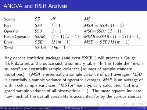
Source SS df MS
Part SSA I − 1 MSA = SSA/ (I − 1)Operator SSB J − 1 MSB=SSB/ (J − 1)Part×Operator SSAB (I − 1) (J − 1) MSAB=SSAB/ (I − 1) (J − 1)Error SSE IJ (m− 1) MSE = SSE/IJ (m− 1)Total SSTot IJm− 1
Any decent statistical package (and even EXCEL) will process a GaugeR&R data set and produce such a summary table. In this table the "meansquares" are essentially sample variances (squares of sample standarddeviations). (MSA is essentially a sample variance of part averages, MSBis essentially a sample variance of operator averages, MSE is an average ofwithin cell-sample variances, "MSTot" isn’t typically calculated, but is agrand sample variance of all observations, ...) The mean squares indicatehow much of the overall variability is accounted for by the various sources.
Vardeman and Morris (Iowa State University) IE 361 Module 6 3 / 21

ANOVA and R&R AnalysisExample 6-1
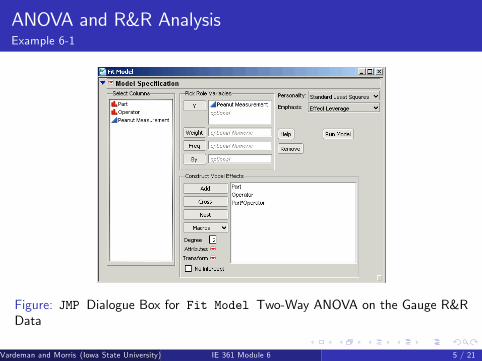
We’ll use the data set with I = 4, J = 3,m = 2 from the in-class R&Rstudy (used as a numerical example in Module 5) to illustrate. The JMPdata table and some screen shots for using the program to get the sums ofsquares follow.
Figure: JMP Data Sheet for the In-Class R&R StudyVardeman and Morris (Iowa State University) IE 361 Module 6 4 / 21
ANOVA and R&R AnalysisExample 6-1
Figure: JMP Dialogue Box for Fit Model Two-Way ANOVA on the Gauge R&RData
Vardeman and Morris (Iowa State University) IE 361 Module 6 5 / 21

ANOVA and R&R AnalysisExample 6-1
Figure: JMP Two-Way ANOVA Report for the In-Class Gauge R&R Study
Vardeman and Morris (Iowa State University) IE 361 Module 6 6 / 21

ANOVA and R&R AnalysisExample 6-1
Although we certainly don’t recommend using EXCEL (a spreadsheet isno substitute for a statistical package and, besides, EXCEL has terriblyunreliable numerical analysis) we found instructions on using the program’stwo-way ANOVA plug-in athttp://www.cvgs.k12.va.us/digstats/main/Guides/g_2anovx.html. Twoscreen shots from using these instructions on the in-class two-way datafollow.
Vardeman and Morris (Iowa State University) IE 361 Module 6 7 / 21

ANOVA and R&R AnalysisExample 6-1
Figure: EXCEL Two-Way Data Spreadsheet for the In-Class R&R Study
Vardeman and Morris (Iowa State University) IE 361 Module 6 8 / 21

ANOVA and R&R Analysis
Figure: EXCEL Two-Way Data Spreadsheet for the In-Class R&R Study
For our present purposes, we will take mean squares and degrees offreedom out of such an ANOVA table and make Gauge R&R estimatesbased on them. Point estimators for the quantities of most interest in aGauge R&R study are partially summarized on the bottom of page 27 inSQAME. These are
Vardeman and Morris (Iowa State University) IE 361 Module 6 9 / 21

ANOVA and R&R Analysis
σrepeatability = σ =√MSE
and
σreproducibility =
√max
(0,MSBmI
+(I − 1)mI
MSAB − 1mMSE
)Although it is not presented in SQAME, an appropriate estimator forσR&R =
√σ2β + σ2αβ + σ2 (that is called σoverall in SQAME ) is
σR&R =
√1mIMSB +
I − 1mI
MSAB +m− 1m
MSE
Vardeman and Morris (Iowa State University) IE 361 Module 6 10 / 21
ANOVA and R&R Analysis
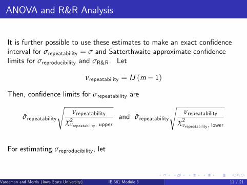
It is further possible to use these estimates to make an exact confidenceinterval for σrepeatability = σ and Satterthwaite approximate confidencelimits for σreproducibility and σR&R. Let
νrepeatability = IJ (m− 1)
Then, confidence limits for σrepeatability are
σrepeatability
√νrepeatability
χ2νrepeatability , upperand σrepeatability
√νrepeatability
χ2νrepeatability , lower
For estimating σreproducibility, let
Vardeman and Morris (Iowa State University) IE 361 Module 6 11 / 21
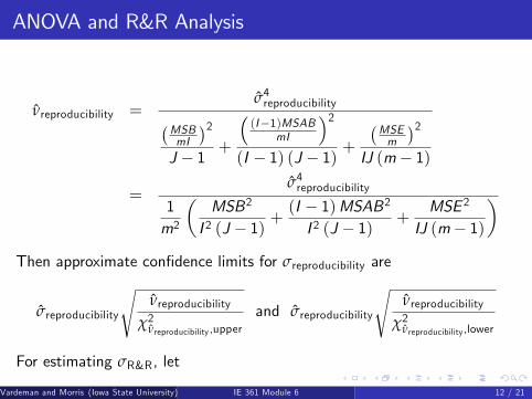
ANOVA and R&R Analysis
νreproducibility =σ4reproducibility(MSB
mI
)2J − 1 +
((I−1)MSAB
mI
)2(I − 1) (J − 1) +
(MSEm
)2IJ (m− 1)
=σ4reproducibility
1m2
(MSB2
I 2 (J − 1) +(I − 1)MSAB2I 2 (J − 1) +
MSE 2
IJ (m− 1)
)Then approximate confidence limits for σreproducibility are
σreproducibility
√νreproducibility
χ2νreproducibility ,upperand σreproducibility
√νreproducibility
χ2νreproducibility ,lower
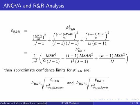
For estimating σR&R, let
Vardeman and Morris (Iowa State University) IE 361 Module 6 12 / 21
ANOVA and R&R Analysis
νR&R =σ4R&R(MSB
mI
)2J − 1 +
((I−1)MSAB
mI
)2(I − 1) (J − 1) +
((m−1)MSE
m
)2IJ (m− 1)
=σ4R&R
1m2
(MSB2
I 2 (J − 1) +(I − 1)MSAB2I 2 (J − 1) +
(m− 1)MSE 2IJ
)then approximate confidence limits for σR&R are
σR&R
√νR&R
χ2νR&R ,upperand σR&R
√νR&R
χ2νR&R ,lower
Vardeman and Morris (Iowa State University) IE 361 Module 6 13 / 21

ANOVA and R&R Analysis
These formulas are tedious (but hardly impossible) to use with a pocketcalculator. There is an EXCEL spreadsheet made by Vanessa Calderon onthe IE 361 web page that can be used to implement these formulas.Vardeman uses a simple MathCAD worksheet to do the computing. Thefollowing figure illustrates the use of that worksheet beginning fromSSB,SSAB,SSE , I , J, and m for the in-class R&R study.
Vardeman and Morris (Iowa State University) IE 361 Module 6 14 / 21
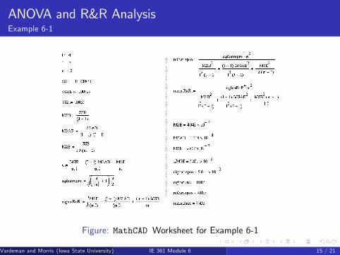
ANOVA and R&R AnalysisExample 6-1
Figure: MathCAD Worksheet for Example 6-1
Vardeman and Morris (Iowa State University) IE 361 Module 6 15 / 21
ANOVA and R&R AnalysisExample 6-1
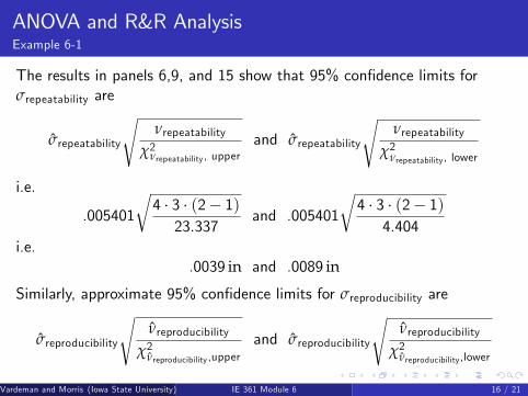
The results in panels 6,9, and 15 show that 95% confidence limits forσrepeatability are
σrepeatability
√νrepeatability
χ2νrepeatability , upperand σrepeatability
√νrepeatability
χ2νrepeatability , lower
i.e.
.005401
√4 · 3 · (2− 1)23.337
and .005401
√4 · 3 · (2− 1)
4.404i.e.
.0039 in and .0089 in
Similarly, approximate 95% confidence limits for σreproducibility are
σreproducibility
√νreproducibility
χ2νreproducibility ,upperand σreproducibility
√νreproducibility
χ2νreproducibility ,lower
Vardeman and Morris (Iowa State University) IE 361 Module 6 16 / 21

ANOVA and R&R AnalysisExample 6-1
i.e.
.009014
√4
11.143and .009014
√4.484
i.e..0054 in and .0259 in
And finally, approximate 95% confidence limits for σR&R are
σR&R
√νR&R
χ2νR&R ,upperand σR&R
√νR&R
χ2νR&R ,lower
i.e.
.011
√7
16.013and .011
√7
1.690
i.e..0073 in and .0224 in
Vardeman and Morris (Iowa State University) IE 361 Module 6 17 / 21
ANOVA and R&R AnalysisExample 6-1
These intervals show that none of these standard deviations are terriblywell-determined (degrees of freedom are small and intervals are wide). Ifbetter information is needed, more data would have to be collected. Butthere is at least some indication that σrepeatability and σreproducibility areroughly of the same order of magnitude. The caliper used to make themeasurements was a fairly crude one, and there were detectabledifferences in the ways the student operators used that caliper.
Vardeman and Morris (Iowa State University) IE 361 Module 6 18 / 21

ANOVA and R&R Analysis
Quite often industrial Gauge R&R studies are done to investigate theadequacy of a measuring device (and the operators that use it) to checkconformance of items produced to engineering specifications (values thatdelineate limits of what is required of the item for it to be functional).Suppose that some feature of a product needs to have a value, x , that isat least L and no more than U in order for it to be functional. (L is thelower specification for x and U is the upper specification.) In this context,it is common to want to compare one’s perception of the size of σR&R to"how tight L and U are." (For example, trying to compare x that can beseen only through a large amount of measurement noise to very tightspecifications is a hopeless task.)
A way of quantifying this kind of comparison is this. If one thinks ofmeasurement error as normally distributed, in the absence of (averageacross operators) measurement bias (µδ = 0), a measurement y made bya "randomly selected" operator in some sense represents x to within
Vardeman and Morris (Iowa State University) IE 361 Module 6 19 / 21
ANOVA and R&R Analysis
±3σR&R and so 6σR&R might be taken as a kind of measurementuncertainty. The difference U − L represents the allowable variation in x .So the ratio
GCR =6σR&RU − L
is sometimes called a Gauge Capability Ratio or a Precision toTolerance Ratio and used as an index of the adequacy of a measurementsystem to verify the functionality of product. Of course, this can only beestimated using the output of a Gauge R&R study, so an estimated versionof this is
GCR =6σR&RU − L
Notice too that having computed confidence limits for σR&R, one needsonly multiply these by
6U − L
in order to produce confidence limits for GCR.Vardeman and Morris (Iowa State University) IE 361 Module 6 20 / 21

ANOVA and R&R Analysis
A common rule of thumb is that one needs to be fairly sure thatGCR < .1 (and preferably that GCR < .01) before a gauge can beconsidered adequate for the purpose of checking conformance of x tospecifications L and U.
Vardeman and Morris (Iowa State University) IE 361 Module 6 21 / 21